Finite-Time Event-Triggered Formation Tracking Control of USVs Subject to Input Saturation Based on Active Disturbance Rejection Control

Abstract

This paper proposes an integrated finite-time relative-threshold event-triggered control (FTRTETC) framework for unmanned surface vehicle (USV) formations under input saturation and unknown time-varying external disturbances. Firstly, a scheme of USV formation control based on signed graph theory is proposed. Next, a Gaussian error function is used to handle input saturation and simplify the backstepping design. Then, a finite-time formation controller is developed based on the active disturbance rejection control (ADRC) method with extended state observers (ESOs) and tracking differentiators (TDs). Also, a relative-threshold event-triggered mechanism is designed to reduce the frequency of control execution and communication load. By Lyapunov’s stability theory, the proposed controller is proven to achieve finite-time convergence, ensuring all closed-loop signals achieve global uniform ultimate boundedness (GUUB) and the system is without Zeno behaviour. Finally, numerical simulation examples are presented to validate the effectiveness and robustness of the proposed controller.

1. Introduction

The ocean covers over 70% of the Earth’s surface and plays an important role in human survival and prosperity, yet 95% of it remains unexplored [1]. With increasing attention to ocean exploration in the past two decades, unmanned surface vehicles (USVs) have gradually demonstrated their broad application prospects in the real world. With their advantages of large payload capacity, high flexibility and low cost, USVs have been widely used in marine data collection, ocean resource exploration, search and rescue, and other fields [2]. Over the years, various USV platforms such as the “C-Worker” and “WAM-V” have been deployed for hydrographic surveying and environmental monitoring [2,3,4]. However, due to the limitations of sensors [5], information processing technologies [6], communication technologies [7] and other constraints, it is often difficult for an individual USV to perform complex missions.

To overcome these constraints, the integration of external monitoring technologies, such as High-Frequency Surface Wave Radar (HFSWR), has gained increasing attention. HFSWR is successfully utilized for ship detection and over-the-horizon surveillance [8,9]. Recent developments in bi-frequency high-resolution HFSWRs have demonstrated significant success in detecting challenging targets like small boats by exploiting high-resolution range-Doppler (RD-HR) maps [9]. Incorporating such advanced monitoring data provides a novel way to improve the situational awareness of USV formations. However, achieving robust control of both individual USVs and the USV formation is challenging. First, imprecise USV model parameters (e.g., hydrodynamic coefficients and rotational inertia), and time-varying external disturbances (e.g., wind and waves in marine environments), introduce significant uncertainties into USV motion [2]. In addition, the input saturation related to the output limits of actuators (e.g., maximum output force and torque) combined with high-delay low-bandwidth communication and limited computation resources leads to additional complexity in controller design [10].

These factors have made research on USV formation control a prominent focus [11]. While PID control remains popular for its simplicity but struggles with nonlinear marine environments [12], and the more robust sliding mode control (SMC) suffers from chattering and potential singularities [13], some researchers have been focusing on integrating artificial intelligence (AI)-based control methods to USV formation control, including traditional AI approaches such as rule-based [14] and fuzzy systems [15], and the latest deep learning and reinforcement learning techniques [16]. However, though these latest approaches provide good robustness with simple design processes, they also involve time-consuming iterative processes to update weight matrix and high-dimensional matrix operations that may be impractical for resource-constrained USV platforms [17]. Instead of relying on precise parameters and complex matrix operations, the active disturbance rejection control (ADRC) method uses fully analytical extended state observers (ESOs) and tracking differentiators (TDs) to estimate and actively cancel uncertainties in real time [18]. Various iterations of ADRC, including linear ADRC and high-order ESO-based control, have been successfully applied to handle the “lumped disturbances” in maritime applications [19,20,21]. Nowadays, the ADRC method is widely used in USV control, though there are still some problems that need further research.

Firstly, the backstepping framework used in the ADRC method requires the system to be smooth and differentiable [22]. However, USVs with input saturation problem exhibit strong nonlinear characteristics, making the ADRC method unsuitable. To address this problem, some researchers have proposed using an auxiliary dynamic system (ADS) to compensate for these nonlinearities [23,24,25], while others have explored smooth approximation functions to mitigate the effects of actuator limits [26,27]. However, ADSs cannot provide continuous compensation [28,29]; they can only compensate once during the entire control process [29]. Also, most ADSs are asymptotic rather than finite-time-stable, which is important in real-world applications [30]. On the other hand, smooth approximation functions may unnecessarily modify control inputs even during normal operation, which will influence the performance of USVs.

Also, practical engineering often requires the formation system to converge within a finite time to meet real-time requirements [31], which is particularly suitable for enhancing convergence speed and improving control accuracy in nonlinear systems. Typical finite-time control methods include homogeneous control, which is simple in structure but sensitive to disturbances [32,33,34]; SMC, which divides motion into reaching and sliding phases to improve robustness [35] but suffers from chattering and potential singularities [13]; and the power-integral method. As an extension of the backstepping framework, the power-integral method constructs controllers using power and nonlinear integral terms to build Lyapunov functions for finite-time convergence [36,37]. While it effectively avoids the singularity problems in virtual control laws [38], its design complexity remains a significant challenge [39].

Another critical concern in USV formation control is the efficiency of communication. Traditional time-triggered control schemes, which use a fixed sampling period, often lead to a waste of communication resources, and conventional event-triggered mechanisms (ETMs) use a fixed threshold, which lacks flexibility in highly dynamic marine environments and leads to unnecessary or delayed updates [40]. To address this problem, some researchers introduced relative-threshold mechanisms to adjust thresholds according to real-time states [41,42]. Dynamic event-triggered mechanisms, which utilize internal dynamic variables to further extend the inter-execution intervals, have also gained traction [20,41]. Such mechanisms are essential for heterogeneous formations where different vehicles may have varying sensing and communication capabilities [43]. Zeno behaviour is one of the major problems for ETMs, where the trigger interval asymptotically approaches zero and results in an infinite number of triggering events within a finite time, making the system unstable and physically unimplementable [44]. Therefore, ensuring a positive lower bound of the trigger interval is essential for practical controller design [45].

Integrating finite-time convergence, input saturation, unknown time-varying disturbances, and efficient communication into a unified framework remains a challenging task. Motivated by these considerations, this paper proposes an integrated finite-time relative-threshold event-triggered controller (FTRTETC). The main contribution of this paper lies in the comprehensive integration and adaptation of multiple control strategies to handle the specific constraints of USV formations:

• A USV formation control scheme based on signed graph theory is established to handle communication topologies among USVs.
• A Gaussian error function is utilized to handle the input saturation problem, providing a smooth approximation that avoids the “explosion of complexity” in traditional backstepping and simplifying the design process.
• A finite-time formation tracking controller is developed with ADRC technology and improved ESOs, ensuring rapid convergence under unknown time-varying disturbances.
• A relative-threshold event-triggered mechanism is adapted to reduce communication frequency while ensuring the system is Zeno-free.

The rest of this paper is organized as follows. Formation tracking control for USV problem formulation and the motion model description for the USVs are particularized in Section 2. Then, Section 3 presents the main results, detailing the design of the FTRTETC based on the ADRC method, as well as analysis of stability and Zeno-free behaviour. Simulation results are described to evaluate the control performance in Section 4. Finally, Section 5 contains the conclusions and future work.

Notation: For a matrix $\mathrm{\alpha }={\left[{\alpha }_1, {\alpha }_2, \dots , {\alpha }_n\right]}^{\mathrm{T}}$ and any number $\beta \in ℝ$, we have ${\mathrm{sig}}^{\beta }\left(\mathrm{\alpha }\right)={\left[{\left|{\alpha }_1\right|}^{\beta }\mathrm{sign}\left({\alpha }_1\right), {\left|{\alpha }_2\right|}^{\beta }\mathrm{sign}\left({\alpha }_2\right), \dots , {\left|{\alpha }_n\right|}^{\beta }\mathrm{sign}\left({\alpha }_n\right)\right]}^{\mathrm{T}}$, where $\mathrm{sign}\left(\cdot \right)$ is a standard signum function. $ℝ$ denotes the set of real numbers. $‖\cdot ‖$ is the Euclidean norm. $\mathrm{diag}\left(\cdot \right)$ denotes the diagonal matrix.

2. Problem Formulation and Preliminaries

2.1. USV Dynamic Model

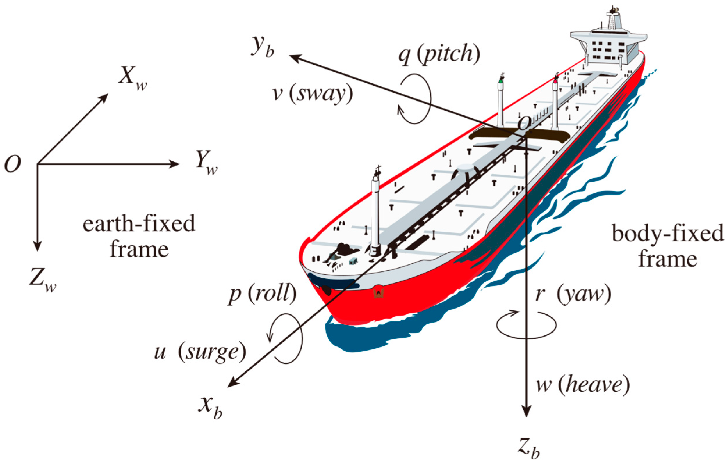
Two rectangular coordinate systems—earth-fixed frame and body-fixed frame—as shown in Figure 1, are used to describe the motion of USVs. Both are right-handed systems, while Newton’s laws of motion only apply to the earth-fixed frame.

In general, a six-degrees-of-freedom (6-DOF) system is used to describe USVs motion and the relationship between position, angle and velocity variables, as shown in Figure 1. According to Remark 1, without loss of generality, a 3-DOF kinematic equation of motion of the USV is described as

$$\dot{\mathrm{\eta }}=\mathrm{J}\left(\psi \right)\mathrm{\upsilon }$$

(1)

where $\mathrm{\eta }={[x, y, \psi ]}^{\mathrm{T}}$ and $\mathrm{\upsilon }={[u, v, r]}^{\mathrm{T}}$. The transformation matrix $\mathrm{J}\left(\psi \right)$ is given by

$$\mathrm{J}\left(\psi \right)=\left[\begin{array}{ccc}\cos \psi & -\sin \psi & 0\\ \sin \psi & \cos \psi & 0\\ 0& 0& 1\end{array}\right]$$

(2)

to describe the relationship between the velocity in the body-fixed frame and the earth-fixed frame.

The dynamic equation of motion of the USV is described as

$$\mathrm{M}\dot{\mathrm{\upsilon }}+\mathrm{C}\left(\mathrm{\upsilon }\right)\mathrm{\upsilon }+\mathrm{D}\left(\mathrm{\upsilon }\right)\mathrm{\upsilon }=\mathrm{\tau }+\mathrm{d}$$

(3)

where $\mathrm{M}>0\in {ℝ}^{3\times 3}$ is the inertia matrix of the rigid body and additional hydrodynamic, $\mathrm{C}\left(\mathrm{\upsilon }\right)\in {ℝ}^{3\times 3}$ is the Coriolis–centripetal matrix, and $\mathrm{D}\left(\mathrm{\upsilon }\right)\in {ℝ}^{3\times 3}$ is the hydrodynamic damping matrix, given by

$$\begin{array}{ccc}\mathrm{M}=\left[\begin{array}{ccc}{m}_{11}& 0& 0\\ 0& m_{22}& m_{23}\\ 0& m_{32}& m_{33}\end{array}\right],& \mathrm{C}\left(\mathrm{\upsilon }\right)=\left[\begin{array}{ccc}0& 0& c_{13}\\ 0& 0& c_{23}\\ -c_{13}& -c_{23}& 0\end{array}\right],& \mathrm{D}\left(\mathrm{\upsilon }\right)=\left[\begin{array}{ccc}{d}_{11}& 0& 0\\ 0& d_{22}& d_{23}\\ 0& d_{32}& d_{33}\end{array}\right]\end{array}$$

(4)

with $m_{11}=m-X_{\dot{u}}$, $m_{22}=m-Y_{\dot{v}}$, $m_{23}=m\cdot x_g-Y_{\dot{r}}$, $m_{32}=m\cdot x_g-N_{\dot{v}}$, $m_{33}=I_z-N_{\dot{r}}$, $c_{13}=-m_{22}v-m_{23}r$, $c_{23}=m_{11}u$, $d_{11}=-X_u-X_{\left|u\right|u}\left|u\right|-X_{uuu}{u}^2$, $d_{22}=-Y_v-Y_{\left|v\right|v}\left|v\right|-Y_{\left|r\right|v}\left|r\right|$, $d_{23}=-Y_r-Y_{\left|v\right|r}\left|v\right|-Y_{\left|r\right|r}\left|r\right|$, $d_{32}=-N_v-N_{\left|v\right|v}\left|v\right|-N_{\left|r\right|v}\left|r\right|$, and $d_{33}=-N_r-N_{\left|v\right|r}\left|v\right|-Y_{\left|r\right|r}\left|r\right|$, where $m$ is the mass of the USV, $I_z$ is the moment of inertia about the yaw rotation, $x_g$ is the distance between the gravity centre of the USV and the origin of body-fixed frame, and $X_{\left(•\right)}$, $Y_{\left(•\right)}$ and $N_{\left(•\right)}$ are hydrodynamic coefficients [47]. $\mathrm{\tau }={[{\tau }_u, {\tau }_v, {\tau }_r]}^{\mathrm{T}}\in {ℝ}^{3\times 1}$ and $\mathrm{d}={[d_u, d_v, d_r]}^{\mathrm{T}}\in {ℝ}^{3\times 1}$ are the input forces and torques of the USV actuators and time-varying external disturbances, respectively.

For a USV considering input saturation, the control input is ${\mathrm{\tau }}_{\mathrm{is}}={\left[{\tau }_{\mathrm{is}u}, {\tau }_{\mathrm{is}v}, {\tau }_{\mathrm{is}r}\right]}^{\mathrm{T}}$, given by

$${\tau }_{\mathrm{is}·}=\left\{\begin{array}{cc}\mathrm{sign}\left({\tau }_{\mathrm{c}·}\right){\tau }_{\max ·}& \mathrm{if}\left|{\tau }_{\mathrm{c}·}\right|>{\tau }_{\max ·}\\ {\tau }_{\mathrm{c}·}& \mathrm{if}\left|{\tau }_{\mathrm{c}·}\right|\le {\tau }_{\max ·}\end{array}\right.$$

(5)

with ${\mathrm{\tau }}_{\mathrm{c}}={\left[{\tau }_{\mathrm{c}u}, {\tau }_{\mathrm{c}v}, {\tau }_{\mathrm{c}r}\right]}^{\mathrm{T}}$ as the command control input given by the controller and ${\tau }_{\max }={\left[{\tau }_{\max u}, {\tau }_{\max v}, {\tau }_{\max r}\right]}^{\mathrm{T}}$ as the maximum control forces and torques provided by the actuators.

Assumption 1

([48]). The external disturbance $\mathrm{d}$ in (3) is unknown and time-varying but bounded, and its first-order derivation $‖\dot{d}‖$ is also bounded.

Assumption 2.

The USV parameters $m$, $I_z$, $x_g$, $X_{\left(•\right)}$, $Y_{\left(•\right)}$ and $N_{\left(•\right)}$ in (4) are unknown. 

Remark 1

([49]). Generally speaking, the USV is symmetric about the mid-longitudinal plane $x_{b}o{z}_b$, and its mass distribution is uniform. Also, the USV has a low centre of gravity and is self-stabilizing, so the roll motion is ignored; the USV operates in still water, so the heave and pitch motions are ignored.

Remark 2.

Considering physical characteristics of the marine environment, the energy of external disturbances $d$ is limited. Also, the inertia of the fluid ensures the disturbances only vary with a finite rate of change. Therefore, Assumption 1 is reasonable.

2.2. Graph Theory

The graph theory is used to describe the communication topology between USVs in formation. Considering a USV formation consisting of a virtual leader and $n$ USVs, the formation is represented by a directed graph $\mathcal{G}=\left\{\mathcal{V}, \mathcal{E}\right\}$, where $\mathcal{V}=\left\{0, 1, 2, \dots , n\right\}$ is the vertex set, with each USV in the formation regarded as a vertex, and $\mathcal{E}=\left\{\left(i, j\right)\in \left\{1, 2, \dots , n\right\}\times \mathcal{V}\right\}$ is the edge set, with every information flow between USVs regarded as an edge. Both vertex set $\mathcal{V}$ and edge set $\mathcal{E}$ are nonempty finite sets. The adjacency matrix is used to describe the ability of communication between USVs, defined as $A=[a_{ij}]\in {ℝ}^{\left(n+1\right)\times \left(n+1\right)} \left(i, j=0, 1, 2, \dots , n\right)$ where $a_{ij}=1$ if the i-th USV can receive information from the j-th USV; otherwise, $a_{ij}=0$. In this paper, self-edges are not allowed; that is, $a_{ii}=0$.

Assumption 3

([50]). There exists at least one directional path from the virtual leader to any of the USVs in the formation.

2.3. Control Objectives

The criteria for achieving tracking control is given by [51]

$$\underset{t\to \infty }{\lim }‖p(t)-p_0(t)-\delta (t)‖=0$$

(6)

where $p(t)$ is the USV’s position, $p_0(t)$ is the virtual leader’s position and $\delta (t)$ is the desired offset at time $t$. Inspired by (6), the position-tracking error for the i-th USV to achieve distributed formation control is defined as

$$s_{i1}=\sum _{j=0}^n{a}_{ij}\left(p_i-p_j-{\delta }_{ij}\right) \left(i=1, 2, \dots , n\right)$$

(7)

where $p_0$ is the virtual leader’s position, $p_i$ and $p_j$ are the position of the i-th USV and j-th USV, respectively, and ${\delta }_{ij}=\left({\delta }_i+p_0\right)-\left({\delta }_j+p_0\right)$ is the desired offset. The control objective is to minimize the position-tracking error given by (7) while considering the input saturation of USV actuators. When all the position-tracking errors for the USVs converge to zero, the entire formation reaches the desired geometric pattern and follows the virtual leader’s trajectory.

Assumption 4

([11,24,26,52]). The virtual leader’s position $p_0$ and its first- and second-order derivation are bounded.

3. Main Results

In this section, a FTRTETC for USV formation subject to input saturation is investigated based on the ADRC method. Then, the stability and Zeno-free analysis of the system are also discussed.

In light of (5), the control input ${\tau }_{\mathrm{is}}$ is a piecewise function which is continuous but non-smooth and nonlinear. Thus, the backstepping framework cannot be applied. To solve this problem, a smooth function to approximate input saturation constraints is constructed as

$$\rho \left({\tau }_{\mathrm{c}·}\right)={\tau }_{\max ·}\mathrm{erf}\left({\displaystyle \frac{\sqrt{\pi }{\tau }_{\mathrm{c}·}}{2{\tau }_{\max ·}}}\right)$$

(8)

where $\mathrm{erf}\left(\cdot \right)$ is the Gaussian error function, defined as $\mathrm{erf}\left(x\right)=\left(2/\sqrt{\pi }\right){\displaystyle {\int }_0^x{e}^{-t^2}dt}$.

Remark 3.

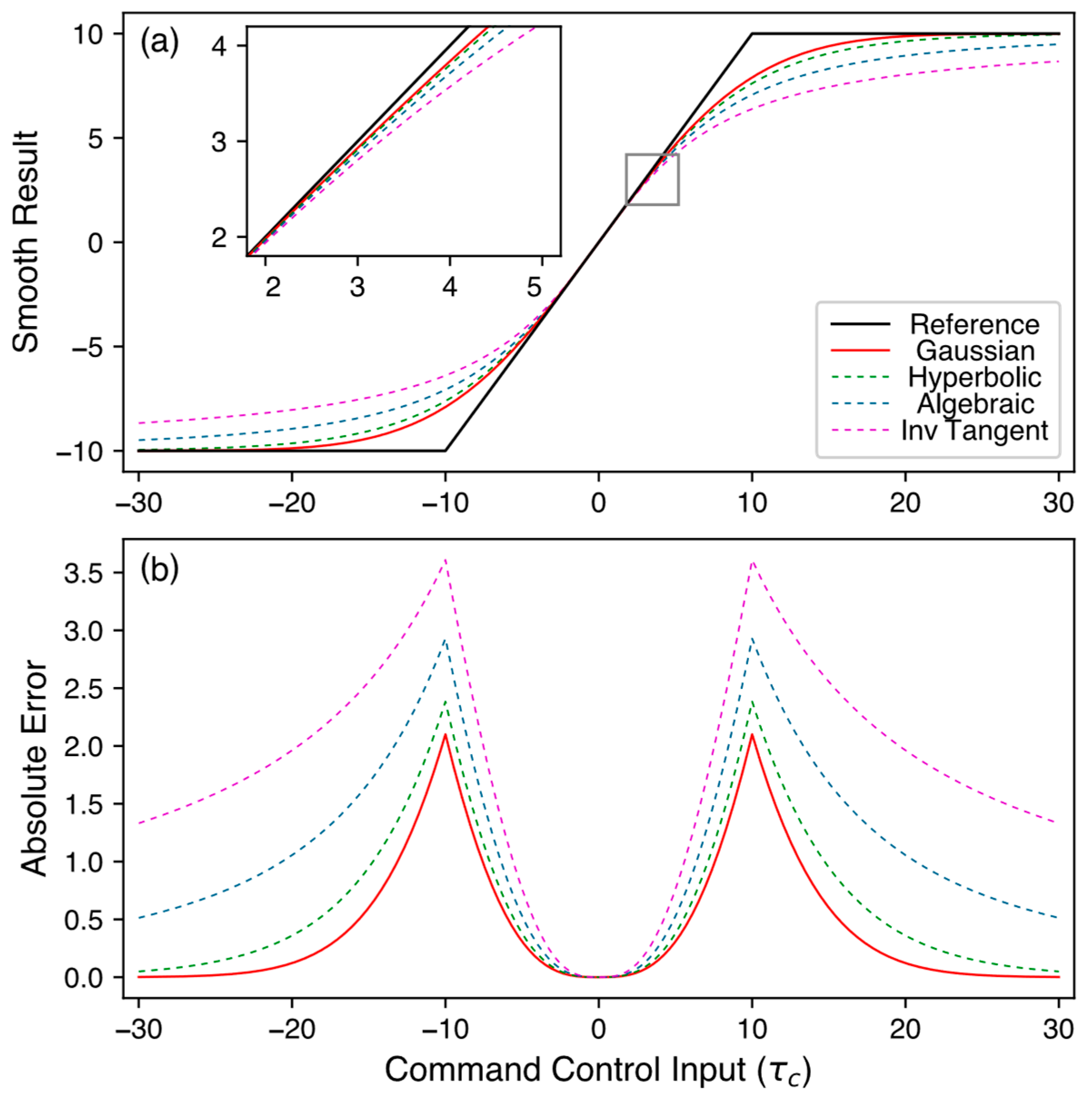
The Gaussian error function and other common smooth functions’ approximation characteristics are shown in Figure 2, where the algebraic function is given by $\tilde{x}=x/\sqrt{1+x^2}$. The Gaussian error function exhibits the fastest convergence rate to the saturation limit and yields the lowest approximation error in the transition region. This justifies the specific selection of the Gaussian error function to reduce residual errors in the backstepping design.

Note the error of input saturation approximation given by

$$e_{\mathrm{is}}\left({\tau }_{\mathrm{c}·}\right)={\tau }_{\mathrm{is}·}-\rho \left({\tau }_{\mathrm{c}·}\right)$$

(9)

is bounded [53]. Thus, we have

$$‖e_{\mathrm{is}}‖=‖\left[e_{\mathrm{is}}\left({\tau }_{\mathrm{c}u}\right), e_{\mathrm{is}}\left({\tau }_{\mathrm{c}v}\right), e_{\mathrm{is}}\left({\tau }_{\mathrm{c}r}\right)\right]‖\le e_{\mathrm{is}m}$$

(10)

with a constant $e_{\mathrm{is}m}>0$.

According to the mean value theorem, we have

$$\rho \left({\tau }_{\mathrm{c}·}\right)=\rho \left(0\right)+{\omega }_{·}{\tau }_{\mathrm{c}·}$$

(11)

where

$${\omega }_{·}=\exp \left(-{\left({\displaystyle \frac{\sqrt{\pi }\iota {\tau }_{\mathrm{c}·}}{2{\tau }_{\max ·}}}\right)}^2\right)>0$$

(12)

for $\forall {\tau }_{\mathrm{c}·}\in ℝ$ with a designed constant $\iota \in \left(0, 1\right)$.

Bringing (9) and (11) into (3), with $\rho \left(0\right)={\tau }_{\max ·}\mathrm{erf}\left(0\right)=0$, the kinematic and dynamic equations of motion of the USV subject to input saturation are given as

$$\left\{\begin{array}{l}\dot{\eta }=J\left(\psi \right)\upsilon \hfill \\ M\dot{\upsilon }+C\left(\upsilon \right)\upsilon +D\left(\upsilon \right)\upsilon =\omega {\tau }_{\mathrm{is}}+d_{\mathrm{is}m}\hfill \end{array}\right.$$

(13)

where $\omega =\mathrm{diag}\left({\omega }_u, {\omega }_v, {\omega }_r\right)$ and $d_{\mathrm{is}m}=d+e_{\mathrm{is}m}$. According to (10) and Assumption 1, $d_{\mathrm{is}m}$ is bounded.

For a relative-threshold event-triggered mechanism $W\left(t\right)=\left[W_u\left(t\right), W_v\left(t\right), W_r\left(t\right)\right]$, the command control input is given by

$${\tau }_{\mathrm{etc}·}\left(t\right)=W_{·}\left(t_k^{·}\right), t\in \left[t_k^{·}, t_{k+1}^{·}\right), k\in {\mathbb{Z}}^{+}$$

(14)

and the event-triggered condition is given by

$$t_{k+1}^{·}=\inf \left\{t\in ℝ|\left|e_{\mathrm{etc}·}\left(t\right)\right|\ge {\hslash }_{·}\left(\cdot \right)\right\}, t_1^{·}=0$$

(15)

where $e_{\mathrm{etc}·}\left(t\right)$ is the error of measurement given by

$$e_{\mathrm{etc}·}\left(t\right)=W_{·}\left(t_k^{·}\right)-{\tau }_{·}\left(t\right)$$

(16)

and ${\hslash }_{·}\left(\cdot \right)$ is a function of the system’s state. When the event-triggered condition given in (15) is triggered, the updating time would be instantaneously set to $t_{k+1}$ and the control input would be instantaneously set to $W_{·}\left(t_{k+1}\right)$ and remain unchanged in the time interval $t\in \left[t_k^{·}, t_{k+1}^{·}\right)$.

Bringing (14) and (16) into (13), the equations of motion of the USV can be further written as

$$\left\{\begin{array}{l}\dot{\eta }=J\left(\psi \right)\upsilon \hfill \\ M\dot{\upsilon }+C\left(\upsilon \right)\upsilon +D\left(\upsilon \right)\upsilon =\omega {\tau }_{\mathrm{etc}}+d_m\hfill \end{array}\right.$$

(17)

where $d_m=d+e_{\mathrm{is}m}+\omega e_{\mathrm{etc}}$. According to (15), $d_m$ is bounded.

Lemma 1

([54]). For any number  $\epsilon >0$ and $\mu \in ℝ$, we have 

$$0\le \left|\mu \right|-\mu \tanh \left({\displaystyle \frac{\mu }{\epsilon }}\right)\le 0.2785\epsilon$$

(18)

where $\tanh \left(\cdot \right)$ is the hyperbolic tangent function.

Lemma 2

([55]). For any number  ${\mathcal{l}}_i\in ℝ \left(i=1, 2, \dots , n\right)$ and $r\in$$\left(0, 1\right)$, we have

$${\left({\displaystyle \sum _{i=1 }^n\left|{\mathcal{l}}_i\right|}\right)}^r\le {\displaystyle \sum _{i=1 }^n{\left|{\mathcal{l}}_i\right|}^r}$$

(19)

Lemma 3

([56]). For any number $c_1>0$,  $c_2>0$  and  $\kappa \in \left(0, 1\right)$, the extended Lyapunov condition of the finite-time stability is given by  $\dot{V}(x)+c_{1}V(x)+c_2{V}^{\kappa }(x)\le 0$, where the settling time is given by 

$$T\le {\displaystyle \frac{1}{c_1\left(1-\kappa \right)}}\ln {\displaystyle \frac{c_1{V}^{1-\kappa }\left(x_0\right)+c_2}{c_2}}$$

(20)

where  $V\left(x_0\right)$  is the initial value.

3.1. Controller Design

The controller design for the i-th USV in the formation contains the following three steps.

Step i, 1: According to (7) and (17), the derivative of position-tracking error $s_{i1}$ is given by

$${\dot{s}}_{i1}=A_{i}J\left({\psi }_i\right){\upsilon }_i+{\Delta }_i+\left(-\sum _{j=0}^n{a}_{ij}{\dot{p}}_j\right)$$

(21)

where $A_i={\displaystyle \sum _{j=0}^n}{a}_{ij}$ and ${\Delta }_i=-A_i{\dot{\delta }}_i+{\displaystyle \sum _{j=0}^n}{a}_{ij}{\dot{\delta }}_j$.

As ${\dot{p}}_0$ and ${\dot{p}}_j$ in (21) are unknown and need to be cancelled, the first ESO is constructed as [57]

$$\left\{\begin{array}{c}{Q}_{iL}={\gamma }_{i1}-s_{i1}\\ {\dot{\gamma }}_{i1}={\gamma }_{i2}-{\sigma }_{i1}{Q}_{iL}+A_{i}J\left({\psi }_i\right){\upsilon }_i+{\Delta }_i\\ {\dot{\gamma }}_{i2}=-{\sigma }_{i2}^2{\mathrm{sig}}^{{\pi }_i}\left(Q_{iL}\right)\end{array}\right.$$

(22)

with designed constants ${\sigma }_{i1}>0$, ${\sigma }_{i2}>0$ and ${\pi }_i\in \left(0, 1\right)$. The ${\gamma }_{i2}$ is the estimation value of $-{\displaystyle \sum _{j=0}^n}{a}_{ij}{\dot{p}}_j$.

To stabilize the position-tracking error, inspired by (22), the first-order virtual velocity controller ${\alpha }_{i1}$ is constructed as

$${\alpha }_{i1}={\displaystyle \frac{J^{\mathrm{T}}\left({\psi }_i\right)}{A_i}}\left(-k_{i1}{s}_{i1}-k_{i10}{S}_i-{\gamma }_{i2}-{\Delta }_i\right)$$

(23)

where $S_i={\left[S_{i,u}, S_{i,v}, S_{i,r}\right]}^{\mathrm{T}}$ is the power function vector to ensure finite-time control. Each component is given by

$$S_{i,·}=\left\{\begin{array}{ll}\mathrm{sign}\left(s_{i1,·}\right)s_{i1,·}^{1/2}\hfill & \mathrm{if} \left|s_{i1,·}\right|\ge {\epsilon }_{i,·}\hfill \\ {\varsigma }_{i1}{s}_{i1,·}+{\varsigma }_{i2}\mathrm{sign}\left(s_{i1,·}\right)s_{i1,·}^3\hfill & \mathrm{if} \left|s_{i1,·}\right|<{\epsilon }_{i,·}\hfill \end{array}\right.$$

(24)

with designed constants $k_{i1}>0$, $k_{i10}>0$, ${\epsilon }_{i,·}>0$ and ${\varsigma }_{i1}=\raisebox{1ex}{$3$}\!\left/ \!\raisebox{-1ex}{$2$}\right.{{\epsilon }_{i,·}}^{\left(\raisebox{1ex}{$-1$}\!\left/ \!\raisebox{-1ex}{$2$}\right.\right)}$, ${\varsigma }_{i2}=\raisebox{1ex}{$-1$}\!\left/ \!\raisebox{-1ex}{$2$}\right.{{\epsilon }_{i,·}}^{\left(\raisebox{1ex}{$-3$}\!\left/ \!\raisebox{-1ex}{$2$}\right.\right)}$.

Remark 4.

In (23), the fractional-order term $S_i$ is introduced to ensure finite-time convergence of the USV formation tracking error. However, in the backstepping design, the time derivative of the virtual controller is required as an input. A singular phenomenon may occur when calculating the time derivative of the virtual controller directly designed as in [36,37] and result in the final controller failing to exist. Therefore, the piecewise function (24) is introduced to ensure the term $k_{i10}{S}_i$ has a continuous and non-singular derivative.

Step i, 2: The velocity-tracking error for a USV to achieve distributed formation control is defined as

$$s_{i2}={\upsilon }_i-{\alpha }_{i1}$$

(25)

and according to (17) and (25), the derivative of $s_{i2}$ is given by

$$\begin{array}{cc}\hfill {\dot{s}}_{i2}& ={\dot{\upsilon }}_i-{\dot{\alpha }}_{i1}\hfill \\ & =M_i^{-1}\left(M_i{\dot{\upsilon }}_i\right)-{\dot{\alpha }}_{i1}\hfill \\ & =-M_i^{-1}C\left({\upsilon }_i\right){\upsilon }_i-M_i^{-1}D\left({\upsilon }_i\right){\upsilon }_i+M_i^{-1}{d}_{im}+M_i^{-1}{\omega }_i{\tau }_{ic}-{\dot{\alpha }}_{i1}\hfill \end{array}$$

(26)

However, solving the derivation of the first-order virtual velocity controller ${\alpha }_{i1}$ directly by a numerical method is difficult. To estimate ${\dot{\alpha }}_{i1}$, the TD is constructed as [22]

$$\left\{\begin{array}{c}{\dot{\chi }}_{i1}={\chi }_{i2}\hfill \\ {\dot{\chi }}_{i2}=-{\phi }_i^2{\mathrm{sig}}^{{\omega }_i}({\chi }_{i1}-{\alpha }_{i1})-{\phi }_i{\chi }_{i2}\hfill \end{array}\right.$$

(27)

with designed constants ${\phi }_i>0$ and ${\omega }_i\in \left(0, 1\right)$. ${\chi }_{i2}$ is the estimated value of ${\dot{\alpha }}_{i1}$.

According to Assumption 2, $C\left({\upsilon }_i\right)$, $D\left({\upsilon }_i\right)$ and $d_i$ in (27) are unknown and need to be cancelled, and the second ESO is constructed as [57]

$$\left\{\begin{array}{cc}\hfill G_{iL}& ={\zeta }_{i1}-{\upsilon }_i\hfill \\ \hfill {\dot{\zeta }}_{i1}& ={\zeta }_{i2}-{∍}_{i1}{G}_{iL}+M_i^{-1}{\omega }_{i0}{\alpha }_{i2}\hfill \\ \hfill {\dot{\zeta }}_{i2}& =-{∍}_{i2}{\mathrm{sig}}^{q_i}\left(G_{iL}\right)\hfill \end{array}\right.$$

(28)

where

$${\omega }_{i0}=\min \left\{{\omega }_{iu}, {\omega }_{iv}, {\omega }_{ir}\right\}>0$$

(29)

in light of (12), with designed constants ${∍}_{i1}>0$, ${∍}_{i2}>0$ and $q_i\in \left(0, 1\right)$. ${\zeta }_{i2}$ is the estimation value of $-M_i^{-1}C\left({\upsilon }_i\right){\upsilon }_i-M_i^{-1}D\left({\upsilon }_i\right){\upsilon }_i+M_i^{-1}{d}_{im}$.

To stabilize the velocity-tracking error, inspired by (28), the second-order controller ${\alpha }_{i2}$ is constructed as

$${\alpha }_{i2}=M_i\left(-k_{i2}{s}_{i2}-k_{i20}{\mathrm{sig}}^{\left(1/2\right)}\left(s_{i2}\right)-{\zeta }_{i2}\right)$$

(30)

with designed constants $k_{i2}>0$ and $k_{i20}>0$.

Step i, 3: The selected relative-threshold event-triggered mechanism and its condition are expressed as

$$\begin{array}{cc}\hfill {\tau }_{i\mathrm{c}·}\left(t\right)=& W_{i·}\left(t_k^{·}\right), t\in \left[t_k^{·}, t_{k+1}^{·}\right), k\in {\mathbb{Z}}^{+}\hfill \\ \hfill t_{k+1}^{·}=& \inf \left\{t\in ℝ|\left|W_{i·}\left(t\right)-{\alpha }_{i2·}\right|\ge {\mathrm{\Pi }}_{i·}\left|{\alpha }_{i2·}\right|+{\upsilon }_{i·}\right\}, t_1^{·}=0\hfill \end{array}$$

(31)

with the designed constant gain ${\mathrm{\Pi }}_{i·}\in \left(0, 1\right)$ and minimum threshold ${\upsilon }_{i·}>0$. Inspired by [41], the controller for i-th USV is designed as

$$W_{i·}\left(t\right)=-\left(1+{\mathrm{\Pi }}_{i·}\right)\left[{\alpha }_{i2·}\tanh \left({\displaystyle \frac{s_{i2·}{\alpha }_{i2·}}{{\mathrm{\Theta }}_{i·}}}\right)+{\overline{\upsilon }}_{i·}\tanh \left({\displaystyle \frac{s_{i2·}{\overline{\upsilon }}_{i·}}{{\mathrm{\Theta }}_{i·}}}\right)\right]$$

(32)

with designed constants ${\mathrm{\Theta }}_{i·}\in ℝ$ and ${\overline{\upsilon }}_{i·}>{\upsilon }_{i·}/\left(1-{\mathrm{\Pi }}_{i·}\right)$.

Remark 5.

To ensure the stability of the closed-loop system under the event-triggered mechanism, the designed controller must be robust against the error of measurement $\left|e_{i\mathrm{etc}·}\left(t\right)\right|=\left|W_{i·}\left(t\right)-{\alpha }_{i2·}\right|<{\mathrm{\Pi }}_{i·}\left|{\alpha }_{i2·}\right|+{\upsilon }_{i·}$ defined in (16). Therefore, the factor  $\left(1+{\mathrm{\Pi }}_{i·}\right)$  is introduced to the designed controller to cancel the relative-threshold gain ${\mathrm{\Pi }}_{i·}$, while the smoothing factor ${\mathrm{\Theta }}_{i\cdot }$  and the robust gain ${\overline{\upsilon }}_{i·}$  are introduced to cancel the disturbance caused by the minimum threshold ${\upsilon }_{i·}$  and ensure the system is without chattering.

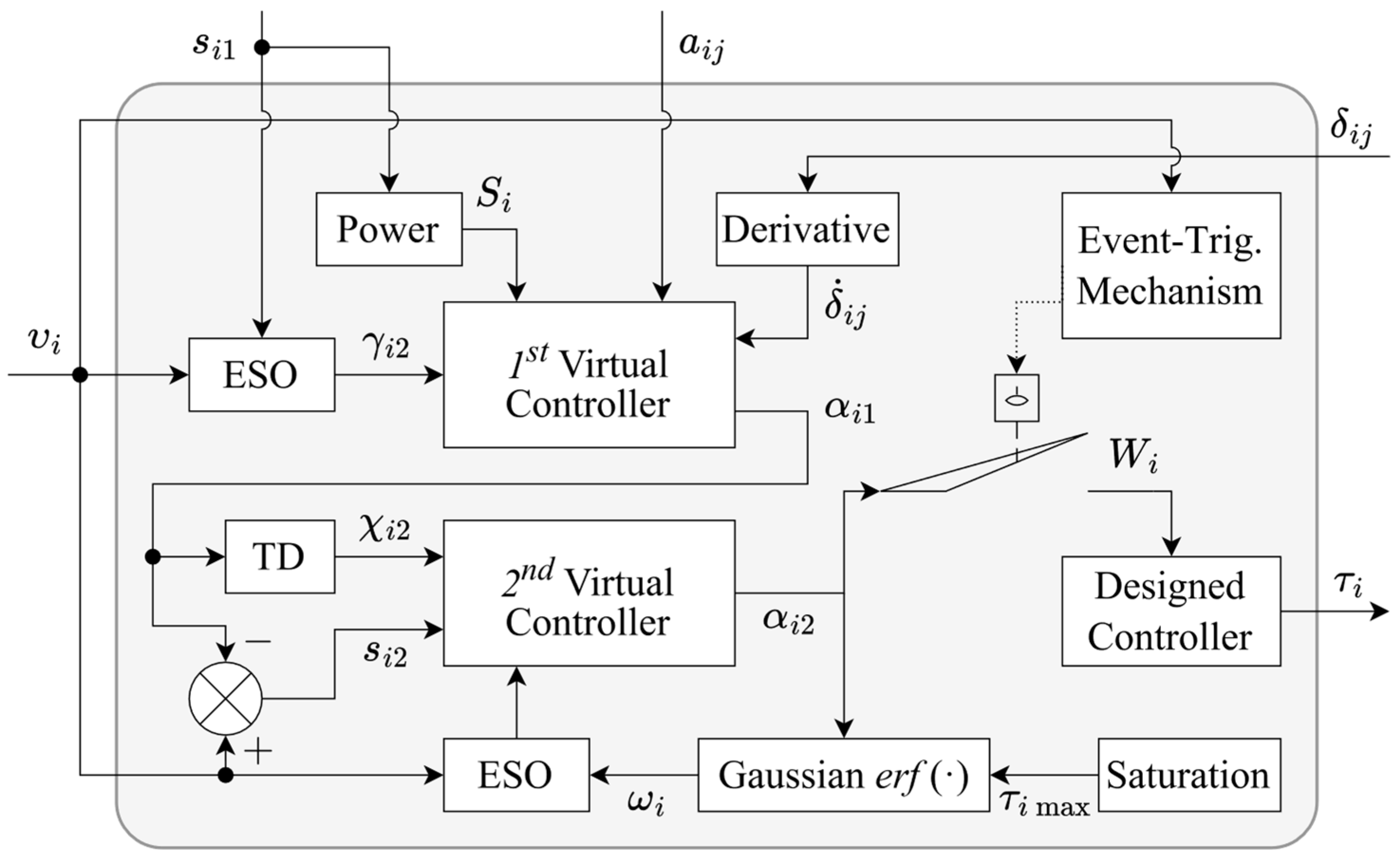
The controller for each USV in the formation is designed by repeating the above steps. The block diagram of the FTRTETCs for the USVs in the formation to achieve finite-time formation tracking control subject to input saturation is shown in Figure 3. In the following section, the stabilization of the control system is discussed.

Remark 6.

As can be seen in the analysis of Theorem 1, the parameter selection of the virtual controller (23) (30) and command controller (32) will directly affect the performance of the proposed controller. The key parameters are$k_{i1}$, $k_{i2}$, $k_{i10}$, $k_{i20}$, ${\mathrm{\Pi }}_{i·}$, ${\mathrm{\Theta }}_{i·}$, and instruction on the selection of parameters for ESOs and TDs can be found in [57] and [22], respectively. $k_{i1}$ and $k_{i2}$ are control gains for finite-time convergence items, and these parameters affect the transient performance of the system. It should be noted that though increasing control gains accelerates the convergence speed, it also increases the magnitude of command control and may cause actuator saturation. $k_{i10}$ and $k_{i20}$ are error feedback control gains used to deal with estimation errors from ESOs and TDs. ${\mathrm{\Pi }}_{i·}$ is the relative-threshold gain used to adjust the maximum allowable deviation between the current output and command control input. ${\mathrm{\Theta }}_{i·}$ is the smoothing factor for hyperbolic tangent functions. It should be noted that although decreasing the smoothing factor ensures higher sensitivity for tracking command control, it may cause chattering.

3.2. Stability and Zeno-Free Analysis

Based on the above design, here are the following theorems and their corresponding proofs.

Theorem 1.

Consider a USV formation that includes multiple USVs, given by (1) and (3), under input saturation, defined as (5), and a relative-threshold event-triggered mechanism, defined as (14) and (15), which satisfies Assumptions 1 to 4, with the ESOs defined as (22) and (28), TDs as in (27), the first-order virtual controller as in (23), the second-order virtual controller as in (30), and the controller as in (31), with the relative-threshold event-triggered condition defined as (32). All signals in the formation system achieve global uniform ultimate boundedness (GUUB), and all USVs can settle to $\mathrm{\Omega }=\left\{s_{i1}|‖s_{i1}‖\le \sqrt{2{\vartheta }_i/{\mathrm{\Gamma }}_i{\mu }_{i1}}\right\}$  with $\mathrm{\Gamma }\in \left(0, 1\right)$. The settling time is given by

$$T_0\le \max \left\{{\displaystyle \frac{4}{(1-{\mathrm{\Gamma }}_i){\mu }_{i1}}}\ln \left({\displaystyle \frac{(1-{\mathrm{\Gamma }}_i){\mu }_{i1}{V}_{i2}^{\left(-1/4\right)}(0)+{\mu }_{i2}}{{\mu }_{i2}}}\right)\right\} \left(i=1, 2, \dots , n\right)$$

(33)

with appropriate design constants.

Proof of Theorem 1.

The Lyapunov function is chosen as

$$\begin{array}{cc}{V}_{i1}={\displaystyle \frac{1}{2}}{s}_{i1}^{\mathrm{T}}{s}_{i1},& {\dot{V}}_{i1}=s_{i1}^{\mathrm{T}}{\dot{s}}_{i1}\end{array}$$

(34)

and

$$\begin{array}{cc}{V}_{i2}=V_{i1}+{\displaystyle \frac{1}{2}}{s}_{i2}^{\mathrm{T}}{s}_{i2},& {\dot{V}}_{i2}={\dot{V}}_{i1}+s_{i2}^{\mathrm{T}}{\dot{s}}_{i2}\end{array}$$

(35)

Bringing (21) into (34), we have

$${\dot{V}}_{i1}=s_{i1}^{\mathrm{T}}\left[-k_{i1}{s}_{i1}-k_{i10}{S}_i+A_i\left({\upsilon }_i-{\alpha }_{i1}\right)+\left(-\sum _{j=0}^n{a}_{ij}{\dot{p}}_j-{\gamma }_{i2}\right)\right]$$

(36)

and bringing (26), (31), and (36) into (35), we have

$$\begin{array}{cc}\hfill {\dot{V}}_{i2}& =s_{i1}^{\mathrm{T}}\left[-k_{i1}{s}_{i1}-k_{i10}{S}_i+A_i\left({\upsilon }_i-{\alpha }_{i1}\right)+\left(-{\displaystyle \sum _{j=0}^n}{a}_{ij}{\dot{p}}_j-{\gamma }_{i2}\right)\right]\hfill \\ & +s_{i2}^{\mathrm{T}}\left[\begin{array}{l}-k_{i2}{s}_{i2}-k_{i20}{\mathrm{sig}}^{\left(1/2\right)}\left(s_{i2}\right)+M_i^{-1}{\omega }_i\left[{\tau }_{i\mathrm{etc}}\left(t\right)-W_i\left(t_{i\mathrm{etc}}^{\ast }\right)\right]\\ +\left(-M_i^{-1}C\left({\upsilon }_i\right){\upsilon }_i-M_i^{-1}D\left({\upsilon }_i\right){\upsilon }_i+M_i^{-1}{d}_{im}-{\zeta }_{i2}\right)-{\chi }_{i2}+\left(-{\dot{\alpha }}_{i1}+{\chi }_{i2}\right)\end{array}\right]\hfill \end{array}$$

(37)

As proved in [57], the ESO estimate errors $-{\displaystyle \sum _{j=0}^n}{a}_{ij}{\dot{p}}_j-{\gamma }_{i2}$ and $-M_i^{-1}C\left({\upsilon }_i\right){\dot{\upsilon }}_i-M_i^{-1}D\left({\upsilon }_i\right){\dot{\upsilon }}_i+M_i^{-1}{d}_i-{\zeta }_{i2}$ are sufficiently small with appropriate design constants. Also, as proved in [22], the TD estimate error $-{\dot{\alpha }}_{i1}+{\chi }_{i2}$ is sufficiently small with appropriate design constants. Thus, the entire error of the ESOs and TDs is defined as ${\xi }_i=\sup \left\{s_{i1}^{\mathrm{T}}\left(-{\displaystyle \sum _{j=0}^n}{a}_{ij}{\dot{p}}_j-{\gamma }_{i2}\right)+s_{i2}^{\mathrm{T}}\left(-M_i^{-1}C\left({\upsilon }_i\right){\upsilon }_i-M_i^{-1}D\left({\upsilon }_i\right){\upsilon }_i+M_i^{-1}{d}_i-{\zeta }_{i2}\right)+s_{i2}^{\mathrm{T}}\left(-{\dot{\alpha }}_{i1}+{\chi }_{i2}\right)\right\}$ and (37) is rewritten as

$$\begin{array}{cc}\hfill {\dot{V}}_{i2}& \le s_{i1}^{\mathrm{T}}\left[-k_{i1}{s}_{i1}-k_{i10}{S}_i+A_i\left({\upsilon }_i-{\alpha }_{i1}\right)\right]\hfill \\ & +s_{i2}^{\mathrm{T}}\left[-k_{i2}{s}_{i2}-k_{i20}{\mathrm{sig}}^{\left(1/2\right)}\left(s_{i2}\right)+M_i^{-1}{\omega }_i\left[{\tau }_{i\mathrm{etc}}\left(t\right)-W_i\left(t_{i\mathrm{etc}}^{\ast }\right)\right]-{\chi }_{i2}\right]+{\xi }_i\hfill \end{array}$$

(38)

As proved in [41], we have

$$W_{i·}\left(t_{i\mathrm{etc}}^{\ast }\right)={\displaystyle \frac{W_{i·}\left(t\right)}{1+{\lambda }_{i1·}{\mathrm{\Pi }}_{i·}}}-{\displaystyle \frac{{\lambda }_{i2·}{\upsilon }_{i·}}{1+{\lambda }_{i1·}{\mathrm{\Pi }}_{i·}}}$$

(39)

with time-varying parameters ${\lambda }_{i1·}$ and ${\lambda }_{i2·}$. Therefore, we have

$$\begin{array}{cc}\hfill s_{i2}^{\mathrm{T}}{W}_i\left(t_{i\mathrm{etc}}^{\ast }\right)& ={\displaystyle \sum _{·}^{u,v,r}}\left[s_{i2·}{W}_{i·}\left(t_{i\mathrm{etc}}^{\ast }\right)\right]\hfill \\ & ={\displaystyle \sum _{·}^{u,v,r}}\left[s_{i2·}\left({\displaystyle \frac{W_{i·}\left(t\right)}{1+{\lambda }_{i1·}{\mathrm{\Pi }}_{i·}}}-{\displaystyle \frac{{\lambda }_{i2·}{\upsilon }_{i·}}{1+{\lambda }_{i1·}{\mathrm{\Pi }}_{i·}}}\right)\right]\hfill \\ & \le {\displaystyle \sum _{·}^{u,v,r}}\left({\displaystyle \frac{s_{i2·}{W}_{i·}\left(t\right)}{1+{\mathrm{\Pi }}_{i·}}}+\left|{\displaystyle \frac{s_{i2·}{\upsilon }_{i·}}{1-{\mathrm{\Pi }}_{i·}}}\right|\right)\hfill \end{array}$$

(40)

and after bringing the relative-threshold event-triggered mechanism $W_{i·}\left(t\right)$ designed in (32) into (40), we further obtain

$$\sum _{·}^{u,v,r}\left({\displaystyle \frac{s_{i2·}{W}_{i·}\left(t\right)}{1+{\mathrm{\Pi }}_{i·}}}+\left|{\displaystyle \frac{s_{i2·}{\upsilon }_{i·}}{1-{\mathrm{\Pi }}_{i·}}}\right|\right)=\sum _{·}^{u,v,r}\left(-s_{i2·}{\alpha }_{i2·}\tanh \left({\displaystyle \frac{s_{i2·}{\alpha }_{i2·}}{{\mathrm{\Theta }}_{i·}}}\right)-s_{i2·}{\overline{\upsilon }}_{i·}\tanh \left({\displaystyle \frac{s_{i2·}{\overline{\upsilon }}_{i·}}{{\mathrm{\Theta }}_{i·}}}\right)+\left|{\displaystyle \frac{s_{i2·}{\upsilon }_{i·}}{1-{\mathrm{\Pi }}_{i·}}}\right|\right)$$

(41)

According to Lemma 1, together with (40) and (41), we have

$$\begin{array}{cc}\hfill s_{i2}^{\mathrm{T}}{W}_i\left(t_{i\mathrm{etc}}^{\ast }\right)& \le {\displaystyle \sum _{·}^{u,v,r}}\left(\left(-\left|s_{i2·}{\alpha }_{i2·}\right|+0.2785\mathrm{\Theta }\right)+\left(-\left|s_{i2·}{\overline{\upsilon }}_{i·}\right|+0.2785\mathrm{\Theta }\right)+\left|{\displaystyle \frac{s_{i2·}{\upsilon }_{i·}}{1-{\mathrm{\Pi }}_{i·}}}\right|\right)\hfill \\ & \le s_{i2}^{\mathrm{T}}{\alpha }_{i2}+1.671\mathrm{\Theta }\hfill \end{array}$$

(42)

In light of the power function vector $S_i$ designed in (24), we have

$$-s_{i1}^{\mathrm{T}}{S}_i=\left\{\begin{array}{ll}-{\displaystyle \sum _{·}^{u,v,r}}{\left|s_{i1,·}\right|}^{\left(3/2\right)}\hfill & \mathrm{if} \left|s_{i1,·}\right|\ge {\epsilon }_{i,·}\hfill \\ -{\displaystyle \sum _{·}^{u,v,r}}{\left|s_{i1,·}\right|}^{\left(3/2\right)}+\sum _{·}^{u,v,r}{f}_i\left(s_{i1,·}\right)\hfill & \mathrm{if} \left|s_{i1,·}\right|<{\epsilon }_{i,·}\hfill \end{array}\right.$$

(43)

with $f_i\left(s_{i1,·}\right)={\varsigma }_{i1}{s}_{i1,·}^2+{\varsigma }_{i2}\mathrm{sign}\left(s_{i1,·}\right)s_{i1,·}^3-{\mathrm{sign}}^{\left(1/2\right)}\left(s_{i1,·}\right)s_{i1,·}$.

In light of (43), $f_i\left(s_{i1,·}\right)$ is bounded for $\left|s_{i1,·}\right|<{\epsilon }_{i,·}$. Therefore, we have ${\displaystyle \sum _{·}^{u,v,r}}{f}_i\left(s_{i1,·}\right)\le {\epsilon }_i^{*}$ with a positive constant ${\epsilon }_i^{*}>0$. According to Lemma 2, we have

$$-s_{i1}^{\mathrm{T}}{S}_i\le -\sum _{·}^{u,v,r}{\left|s_{i1,·}\right|}^{\left(3/2\right)}+{\epsilon }_i^{*}\le -\sum _{·}^{u,v,r}{\left(s_{i1,·}^2\right)}^{\left(3/4\right)}+{\epsilon }_i^{*}=-{\left(s_{i1}^{\mathrm{T}}{s}_{i1}\right)}^{\left(3/4\right)}+{\epsilon }_i^{*}$$

(44)

After expanding (38), substituting (42) and (44) into it, we have

$$\begin{array}{cc}\hfill {\dot{V}}_{i2}& \le -s_{i1}^{\mathrm{T}}{k}_{i1}{s}_{i1}-k_{i10}{\left(s_{i1}^{\mathrm{T}}{s}_{i1}\right)}^{\left(3/4\right)}+k_{i10}{\epsilon }_i^{*}+s_{i1}^{\mathrm{T}}{A}_i\left({\upsilon }_i-{\alpha }_{i1}\right)\hfill \\ & -s_{i2}^{\mathrm{T}}{k}_{i2}{s}_{i2}-k_{i20}{\left(s_{i2}^{\mathrm{T}}{s}_{i2}\right)}^{\left(3/4\right)}+s_{i2}^{\mathrm{T}}{M}_i^{-1}{\omega }_i\left({\tau }_{i\mathrm{etc}}-{\alpha }_{i2}\right)-1.671M_i^{-1}{\omega }_i\mathrm{\Theta }-s_{i2}^{\mathrm{T}}{\chi }_{i2}+{\xi }_i\hfill \\ & \le -{\mu }_{i1}{V}_{i2}-{\mu }_{i2}{V}_{i2}^{\left(3/4\right)}+{\vartheta }_i\hfill \end{array}$$

(45)

with ${\mu }_{i1}=\min \left\{2k_{i1}, 2k_{i2}\right\}$, ${\mu }_{i2}=\min \left\{2^{\left(3/4\right)}{k}_{i10}, 2^{\left(3/4\right)}{k}_{i20}\right\}$ and ${\vartheta }_i=k_{i10}{\epsilon }_i^{*}+s_{i1}^{\mathrm{T}}{A}_i\left({\upsilon }_i-{\alpha }_{i1}\right)+s_{i2}^{\mathrm{T}}{M}_i^{-1}\left({\tau }_{i\mathrm{etc}}-{\alpha }_{i2}\right)-1.671M_i^{-1}{\omega }_i\mathrm{\Theta }-s_{i2}^{\mathrm{T}}{\chi }_{i2}+{\xi }_i$.

Furthermore, by decomposing ${\mu }_{i1}=\mathrm{\Gamma }{\mu }_{i1}+\left(1-\mathrm{\Gamma }\right){\mu }_{i1}$ where $\mathrm{\Gamma }\in \left(0, 1\right)$, we have

$${\dot{V}}_{i2}\le -\mathrm{\Gamma }{\mu }_{i1}{V}_{i2}-\left(1-\mathrm{\Gamma }\right){\mu }_{i1}{V}_{i2}-{\mu }_{i2}{V}_{i2}^{\left(3/4\right)}+{\vartheta }_i$$

(46)

and if $V_{i2}\le \left({\vartheta }_i/\mathrm{\Gamma }{\mu }_{i1}\right)$, in light of (46), we have ${\dot{V}}_{i2}\le -\left(1-\mathrm{\Gamma }\right){\mu }_{i1}{V}_{i2}-{\mu }_{i2}{V}_{i2}^{\left(3/4\right)}$. According to Lemma 3, the settling time is given as

$$T_i\le {\displaystyle \frac{4}{(1-{\mathrm{\Gamma }}_i){\mu }_{i1}}}\ln \left({\displaystyle \frac{(1-{\mathrm{\Gamma }}_i){\mu }_{i1}{V}_{i2}^{\left(-1/4\right)}(0)+{\mu }_{i2}}{{\mu }_{i2}}}\right)$$

(47)

with $V_2\left(0\right)$ as the initial value of $V_2$. Moreover, in light of (35), we have $\frac{1}{2}{s}_{i2}^{\mathrm{T}}{s}_{i2}\le V_{i2}\le \left({\vartheta }_i/\mathrm{\Gamma }{\mu }_{i1}\right)$ and thus $‖s_{i1}‖\le \sqrt{2{\vartheta }_i/{\mathrm{\Gamma }}_i{\mu }_{i1}}$. The other signals in the closed-loop system are easily proven to be bounded [26], and the settling time for the USV formation is given as $T_0\le \max \left\{T_i\right\} \left(i=1, 2, \dots , n\right)$.

This completes the proof. □

Theorem 2.

Consider a USV formation that includes multiple USVs, given by (1) and (3), under input saturation, defined as (5), and a relative-threshold event-triggered mechanism, defined as (14) and (15), which satisfies Assumptions 1 to 4, with the ESOs defined as (22) and (28), TDs as in (27), the first-order virtual controller as in (23), the second-order virtual controller as in (30), and the controller as in (31), with the relative-threshold event-triggered condition defined as (32). The formation system is Zeno-free with any trigger time interval $t_{k+1}-t_k>0$.

Proof of Theorem 2.

Consider a single DOF of the i-th USV in the formation; assume it has triggered the update condition for $k$ time(s) and the last trigger time is $t_k^{·}$. In light of (32), in the time interval $t\in \left[t_k, t_{k+1}\right)$, the error of measurement is given by

$$e_{i\mathrm{etc}·}\left(t\right)=W_{i·}\left(t\right)-{\tau }_{i\mathrm{c}·}\left(t\right)$$

(48)

and the partial derivation of $\left|e_{i\mathrm{etc}·}\left(t\right)\right|$ is given by

$$\frac{\partial }{\partial t}\left|e_{i\mathrm{etc}·}\left(t\right)\right|=\frac{\partial }{\partial t}{\left[e_{i\mathrm{etc}·}\left(t\right)\times e_{i\mathrm{etc}·}\left(t\right)\right]}^{{\displaystyle \frac{1}{2}}}=\mathrm{sign}\left(e_{i\mathrm{etc}·}\left(t\right)\right)\cdot {\dot{e}}_{i\mathrm{etc}·}\left(t\right)\le \left|{\dot{W}}_{i·}\left(t\right)\right|$$

(49)

with both $W_{i·}\left(t\right)$ and ${\dot{W}}_{i·}\left(t\right)$ proved to be bounded in Theorem 1. Thus, we have

$$\frac{\partial }{\partial t}\left|e_{i\mathrm{etc}·}\left(t\right)\right|\le \left|{\dot{W}}_{i·}\left(t\right)\right|\le {\mathrm{\Xi }}_{i·}$$

(50)

with a constant ${\mathrm{\Xi }}_{i·}\ge 0$.

In light of (31), we have

$$e_{i\mathrm{etc}·}\left(t_k^{·}\right)=0$$

(51)

and

$$\underset{t\to t_{k+1}^{·}}{\lim }{e}_{i\mathrm{etc}·}\left(t\right)={\mathrm{\Pi }}_{i·}\left|{\tau }_{i\mathrm{c}·}\left(t\right)\right|+{\upsilon }_{i·}$$

(52)

According to the mean value theorem, and in light of (49), (50) and (51), we have

$$e_{i\mathrm{etc}·}\left(t_{k+1}^{·}\right)=e_{i\mathrm{etc}·}\left(t_k^{·}\right)+\frac{\partial }{\partial t}\left|e_{i\mathrm{etc}·}\left(t\right)\right|\left(t_{k+1}^{·}-t_k^{·}\right)\le {\mathrm{\Xi }}_{i·}\left(t_{k+1}^{·}-t_k^{·}\right)$$

(53)

and in light of (52), we have

$$t_{k+1}^{·}-t_k^{·}\ge {\displaystyle \frac{{\mathrm{\Pi }}_{i·}\left|{\tau }_{i\mathrm{c}·}\left(t\right)\right|+{\upsilon }_{i·}}{{\mathrm{\Xi }}_{i·}}}>0$$

(54)

which means that any trigger time interval is larger than 0. The behaviour of each DOF of each USV in the formation is proved by repeating the above steps, and thus the formation system is Zeno-free.

This completes the proof. □

4. Simulation Results

In this section, numerical simulation is implemented to evaluate the effectiveness and robustness of the proposed FTRTETC. The proposed FTRTETC is applied to control the formation to follow the desired trajectory of the virtual leader while maintaining the predefined formation pattern.

4.1. Basic Parameter Setting

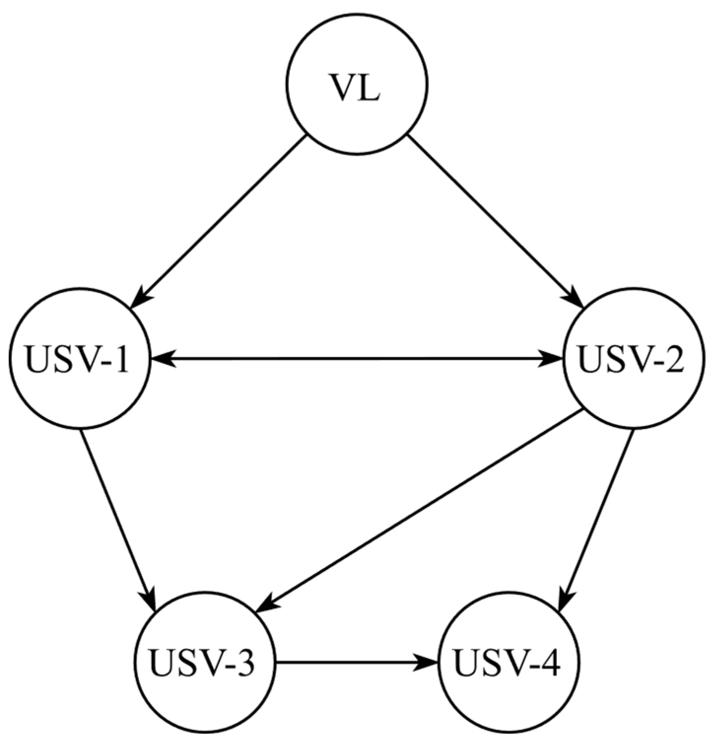
A formation consisting of four USVs was used, and the interactions among them are illustrated in Figure 4. USV-1 and USV-2 can get the virtual leader’s position directly, while USV-3 and USV-4 are inaccessible. This configuration forms a hierarchical communication structure, where USV-1 and USV-2 are the primary followers, and USV-3 and USV-4 are the secondary followers.

Some accurately determined parameters relevant to USVs used for simulation (refer to [52]) are listed in

Table 1. Values of USVs parameters [52].

Parameters	Values	Parameters	Values	Parameters	Values
$m$	23.8000	$Y_v$	−0.8612	$X_{\dot{u}}$	−2.0000
$I_z$	1.7600	$Y_{\left|v\right|v}$	−36.2823	$Y_{\dot{v}}$	−10.0000
$x_g$	0.0460	$Y_r$	0.1079	$Y_{\dot{r}}$	0.0000
$X_u$	−0.7225	$N_v$	0.1052	$N_{\dot{v}}$	0.0000
$X_{\left|u\right|u}$	−1.3274	$N_{\left|v\right|v}$	5.0437	$N_{\dot{r}}$	−1.0000
$X_{uuu}$	−5.8664

, while the remaining undetermined hydrodynamic parameters ${[Y_{\left|r\right|v}, Y_{\left|v\right|r}, Y_{\left|r\right|r}, N_{\left|r\right|v}, N_r, N_{\left|v\right|r}, N_{\left|r\right|r}, b_1, b_2, b_3]}^{\mathrm{T}}$ are modelled as $-0.2C\left(\upsilon \right)\upsilon -0.2D\left(\mathrm{\upsilon }\right)\mathrm{\upsilon }$ [58]. The corresponding input saturation limits are $\left|{\tau }_u\right|, \left|{\tau }_v\right|\le 20.0 \mathrm{N}$ and $\left|{\tau }_r\right|\le 15.0 \mathrm{N}\cdot \mathrm{m}$ [52].

The desired trajectory of the USV formation is generated by the virtual leader (indexed as 0), which serves as the reference tracking objective for the group. The reference motion of the virtual leader is defined as $x_0=0.5t$ and $y_0=0.5\sin \left(0.5t\right)$. Accordingly, its velocity components are given by $v_{x_0}=d{x}_0/dt$ and $v_{y_0}=d{y}_0/dt$, and the reference yaw angle is given by ${\psi }_0=\arctan \left(v_{y_0}/v_{x_0}\right)=\arctan \left(\cos \left(0.5t\right)/2\right)$. Consequently, the complete desired trajectory vector is represented as ${\mathrm{p}}_0={\left[x_0, y_0, {\psi }_0\right]}^{\mathrm{T}}$.

The desired offsets of the four follower USVs were chosen as

$$\left\{\begin{array}{c}{\mathrm{\delta }}_{10}={\left[\begin{array}{ccc}-3& 3& 0\end{array}\right]}^{\mathrm{T}}\\ {\mathrm{\delta }}_{20}={\left[\begin{array}{ccc}-3& 5& 0\end{array}\right]}^{\mathrm{T}}\\ {\mathrm{\delta }}_{30}={\left[\begin{array}{ccc}-9& 7& 0\end{array}\right]}^{\mathrm{T}}\\ {\mathrm{\delta }}_{40}={\left[\begin{array}{ccc}-9& 9& 0\end{array}\right]}^{\mathrm{T}}\end{array}\right.$$

(55)

and all USVs were initialized with positions given in

Table 2. Initial positions of USVs.

Index	Items
	x [m]	y [m]	ψ [rad]
USV-1	−3.15881	3.04075	0.14899
USV-2	2.93382	4.90127	0.08363
USV-3	−8.89148	6.96558	−0.06767
USV-4	8.77815	8.91604	−0.40011

and zero initial velocity. The designed parameters for the FTRTETC are listed in

Table 3. Designed FTRTETC parameters.

Parameters	Values	Parameters	Values	Parameters	Values
${\sigma }_{\ast 1}$	40.00	$k_{\ast 1}$	5.00	$k_{\ast 2}$	3.50
${\sigma }_{\ast 2}$	1.00	$k_{\ast 10}$	15.00	$k_{\ast 20}$	0.10
${\pi }_{\ast }$	0.10	${\epsilon }_{\ast }$	50.00	${\mathrm{\Theta }}_{\ast ·}$	0.30
${∍}_{\ast 1}$	40.00	${\iota }_{\ast }$	0.01	${\mathrm{\Pi }}_{\ast ·}$	0.10
${∍}_{\ast 2}$	1.00	${\phi }_{\ast }$	1.00	${\upsilon }_{\ast ·}$	0.30
$q_{\ast }$	0.20	${\omega }_{\ast }$	0.90	${\overline{\upsilon }}_{\ast ·}$	0.50

, and the unknown time-varying external disturbances acting on these follower USVs were chosen as

$$\mathrm{d}=\left[\begin{array}{l}15\cos \left(0.1\mathsf{\pi }t-\mathsf{\pi }/3\right)\\ 15\cos \left(0.2\mathsf{\pi }t+\mathsf{\pi }/2\right)\\ 2\cos \left(0.1\mathsf{\pi }t+\mathsf{\pi }/6\right)\end{array}\right]$$

(56)

The simulation experiment was conducted on a computational platform running the 64-bit Windows 10 Enterprise operating system (version 22H2, OS build 19045.5608), equipped with 128 GB of memory and a 32-core Intel(R) Xeon(R) Platinum 8370C CPU operating at a base frequency of 2.80 GHz. The total simulation time was 100 s, with a minimum simulation time step of 0.001 s.

4.2. Formation Trajectory-Tracking Performance

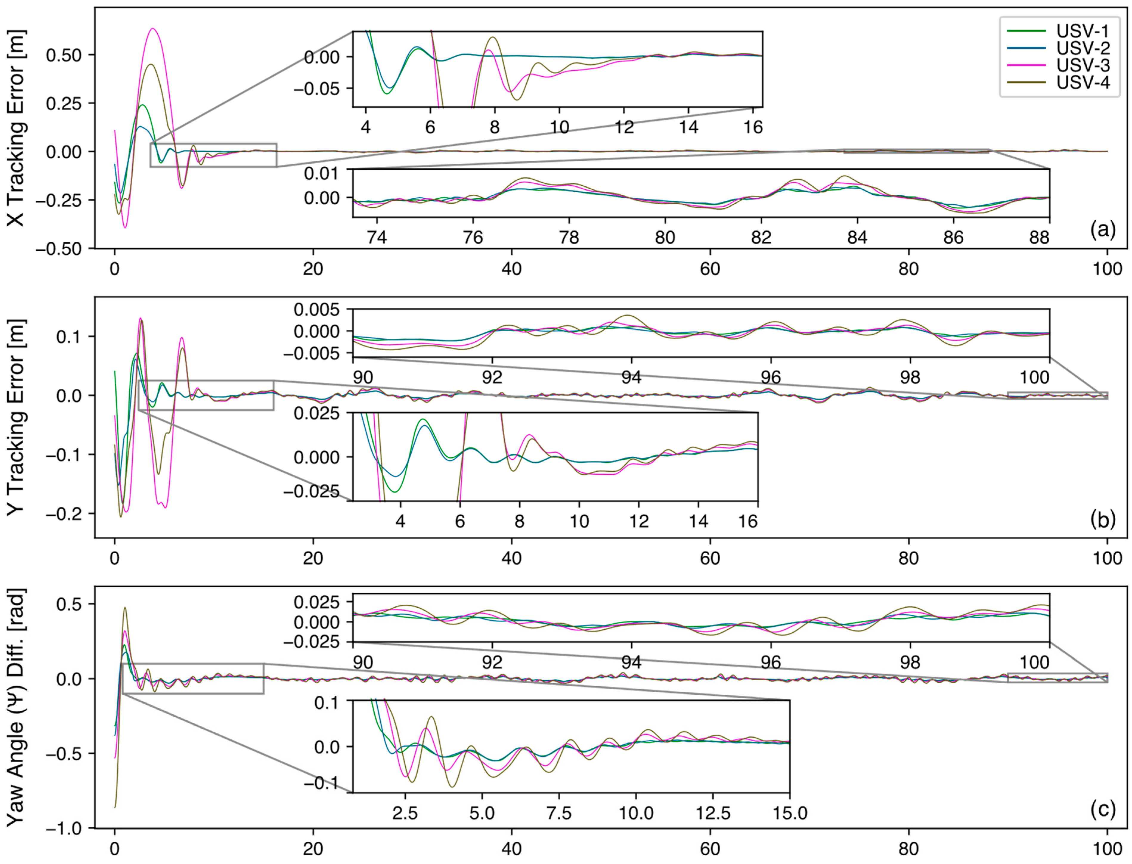
The position-tracking error curves of the follower USVs are shown in Figure 5, which are calculated according to the distributed position-tracking error defined by (7). The different initial positions listed in Table 2 lead to different initial tracking errors. The tracking errors in each DOF converge to a neighbourhood of zero, indicating that all the follower USVs achieve stable tracking under the proposed FTRTETC. The quantitative tracking performance of each follower USV is shown in

Table 4. Quantitative tracking performance of USVs.

Index	DOF	Criteria
		Settling Time [s]	Maximum Error [m or rad]	Steady-State Error [m or rad]	Steady-State Error Percentage
USV-1	$x$	6.517	−0.004980	0.001410	0.0470%
	$y$	5.321	0.007255	0.001932	0.0644%
	$\psi$	3.079	−0.030606	0.005896
USV-2	$x$	6.502	−0.004983	0.001416	0.0472%
	$y$	5.255	0.007412	0.001979	0.0396%
	$\psi$	3.154	−0.030855	0.005977
USV-3	$x$	12.363	0.008079	0.002154	0.0239%
	$y$	8.515	0.011649	0.003030	0.0433%
	$\psi$	12.547	−0.030754	0.009084
USV-4	$x$	11.628	0.010452	0.002607	0.0290%
	$y$	8.371	0.014283	0.003792	0.0421%
	$\psi$	12.846	0.041075	0.011302

. The settling time is estimated and can be read directly from Figure 5, while the steady-state error is calculated as the mean absolute tracking error over the final 30% of the simulation time. The maximum tracking error is measured between the estimated settling time and the end of the simulation, and its sign indicates the deviation direction only. The primary followers USV-1 and USV-2 reach a steady state within approximately 6.5 s, while the secondary followers USV-3 and USV-4 converge slightly later at around 12.5 s. Despite the input saturation limits, imprecise USV model parameters, and time-varying external disturbances, the steady-state error remains remarkably small—the maximum steady-state error is only 0.06% in the y-direction for USV-1. These results clearly demonstrate the effectiveness and robustness of the proposed FTRTETC in achieving accurate and stable formation tracking.

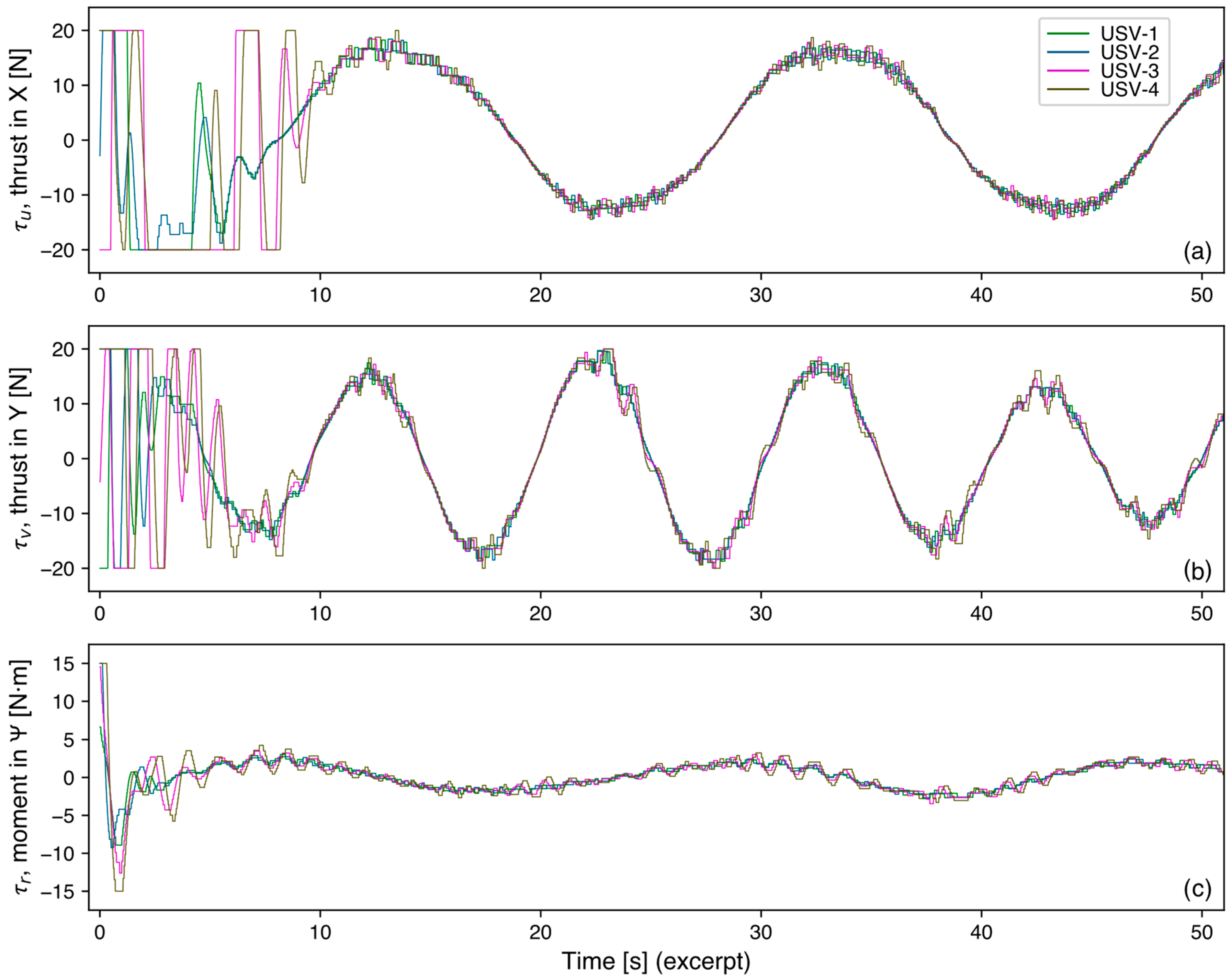
The control inputs in surge, sway and yaw under input saturation are shown in Figure 6. Apart from the significant changes in the initial state (0–10 s), the inputs remain relatively stable. The control inputs are successfully limited within the predefined saturation limits, validating the effectiveness of using the Gaussian error function as a compensation mechanism for input saturation. In addition, the dynamic system reaches surge-input stability at approximately 4 s for USV-1/2 and 7 s for USV-3/4. As shown in Figure 6 and Table 4, the settling time of the dynamic system is shorter than that of the kinematic system, thereby ensuring fast convergence of the overall formation control system. Moreover, the zoomed-in regions of each subplot demonstrate the effectiveness of the proposed relative-threshold event-triggered mechanism in reducing the update frequency of the control inputs.

4.3. Extended State Observer Performance

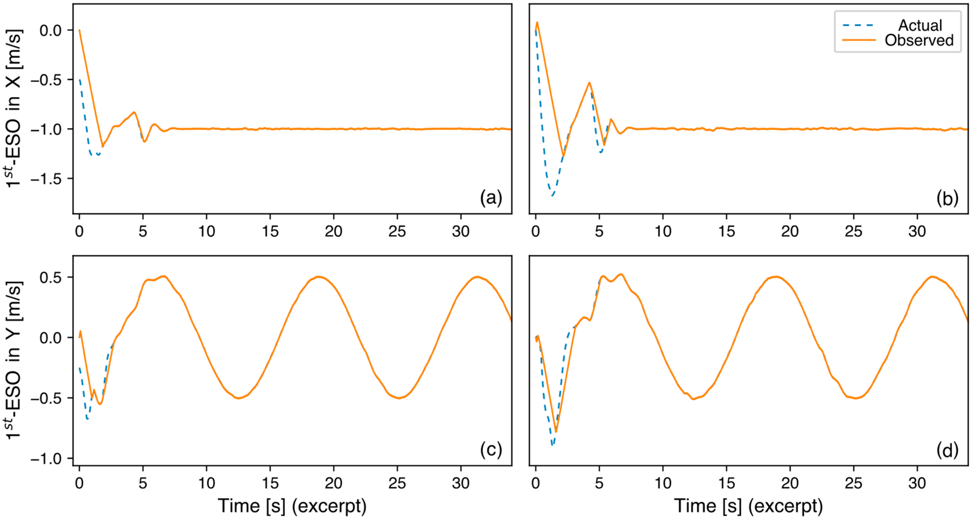
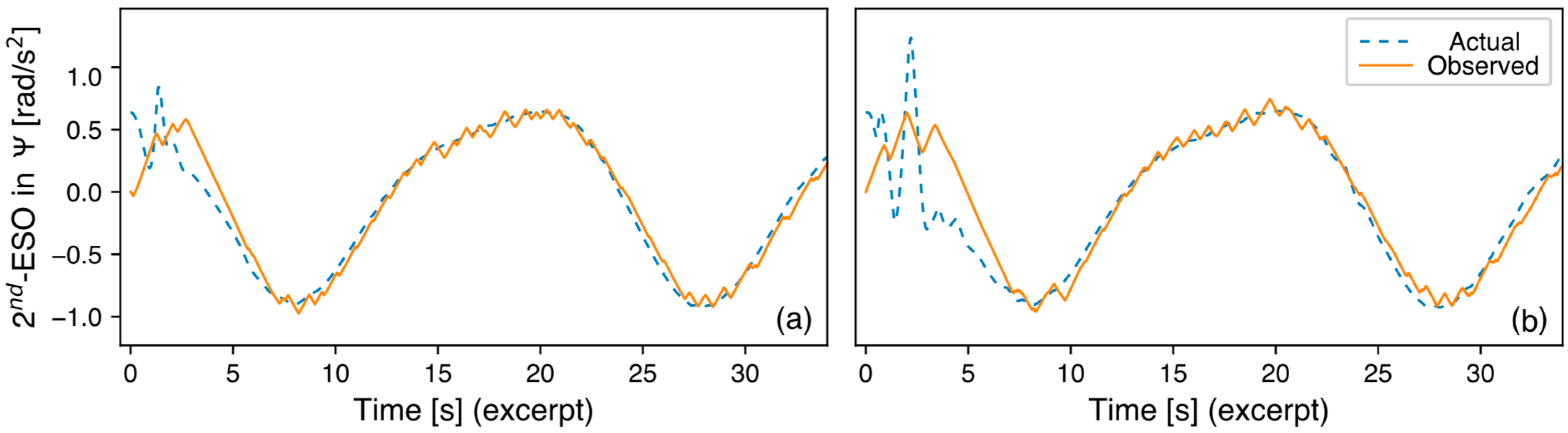
Excerpted ESO observation results for the first- and second-order unknown disturbances of USVs are shown in Figure 7 and Figure 8, respectively. The settling time is approximately 4 s for the first ESO and 7 s for the second ESO, demonstrating the observers’ ability to provide quick estimation of unknown states even when starting from different initial tracking errors. After the initial transient phase, the proposed ESOs can accurately estimate the value of unknown time-varying disturbances, where the observed values and the actual values are same, with negligible estimation error. Furthermore, the results show minimal phase lag, which is critical for ADRC to effectively cancel disturbances in real time. These results validate the effectiveness of the ESO structures designed in (22) and (28).

4.4. Event-Triggered Mechanism Performance

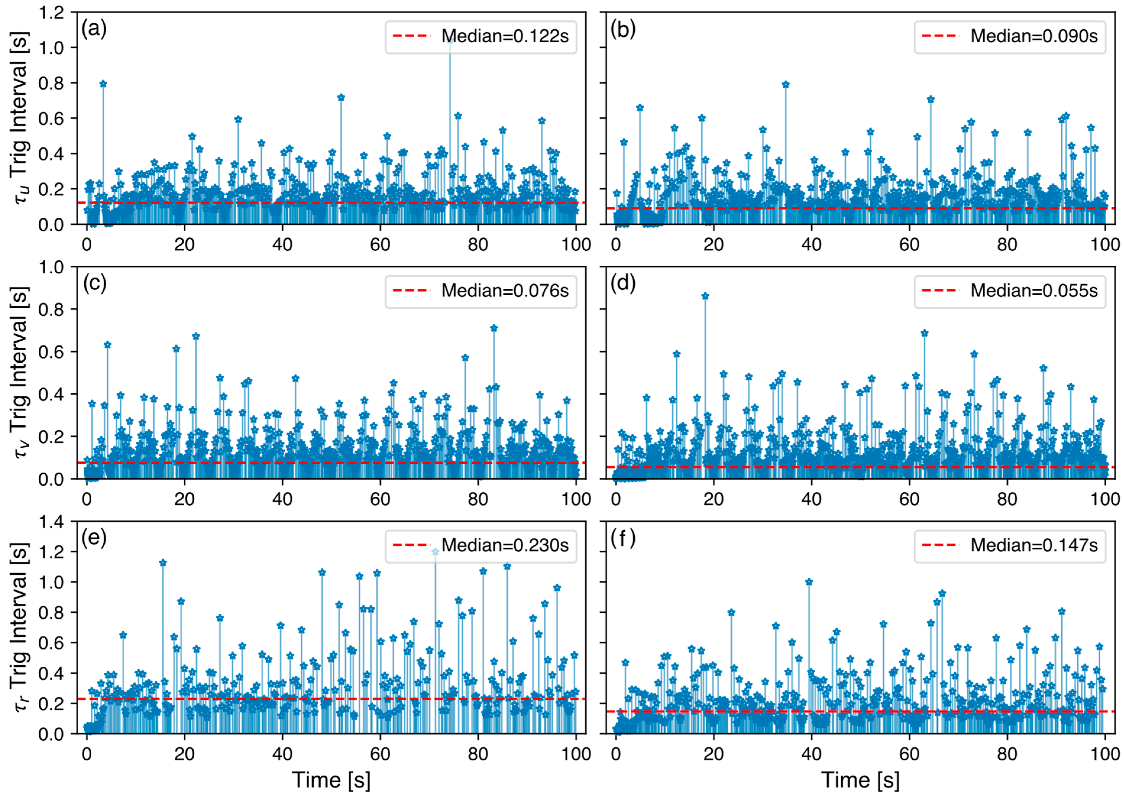
The update intervals of control inputs for follower USV-1 are shown in Figure 9. The counts of triggering events and median trigger intervals are summarized in

Table 5. Statistical summary of two event-triggered mechanisms.

Index	DOF	FTRTETC		Fixed-Threshold ETC
		Median Interval [s]	Event Count	Event Count	Percentage Difference
USV-1	${\tau }_u$	0.122	725	1059	−31.54%
	${\tau }_v$	0.076	987	1061	−6.97%
	${\tau }_r$	0.230	366	366	0.00%
USV-2	${\tau }_u$	0.111	728	789	−7.73%
	${\tau }_v$	0.072	991	1097	−9.66%
	${\tau }_r$	0.219	365	386	−5.44%
USV-3	${\tau }_u$	0.090	933	2485	−62.45%
	${\tau }_v$	0.055	1251	1522	−17.81%
	${\tau }_r$	0.147	528	573	−7.85%
USV-4	${\tau }_u$	0.072	1026	1351	−24.06%
	${\tau }_v$	0.052	1279	1570	−18.54%
	${\tau }_r$	0.089	754	824	−8.50%

. In general, the yaw control inputs have the longest trigger intervals, and the sway control inputs have the shortest trigger intervals, from 0.052 to 0.076 s, especially for secondary followers USV-3 and USV-4. The minimum time interval between any two triggering events is guaranteed to be greater than zero, demonstrating that the formation system under the proposed FTRTETC is Zeno-free. Furthermore, as shown in Figure 6, the control inputs only update when the event-triggering condition is satisfied. Therefore, the proposed event-triggered mechanism is effective and efficient.

To further verify the effectiveness of the proposed relative-threshold event-triggered mechanism, a fixed-threshold event-triggered condition from [24] was used to replace the relative-threshold event-triggering condition defined in (32) in the FTRTETC. The fix-threshold event-triggered controller (ETC) is designed as

$${\tau }_{\mathrm{c}·}\left(t\right)={\alpha }_{2·}\left(t_k^{·}\right), t\in \left[t_k^{·}, t_{k+1}^{·}\right), k\in {\mathbb{Z}}^{+}$$

(57)

and the event-triggered condition is given by

$$t_{k+1}^{·}=\inf \left\{t\in ℝ|\left|{\alpha }_{2·}\left(t_k^{·}\right)-{\tau }_{\mathrm{c}·}\left(t\right)\right|\ge {\mathrm{\Xi }}_{·}\right\}, t_1^{·}=0$$

(58)

with a designed constant threshold $\mathrm{\Xi }\in {ℝ}^{3\times 1}$. By adjusting the threshold, the performance of the fixed-threshold ETC is comparable to that of the FTRTETC. The designed threshold is $\mathrm{\Xi }={\left[0.950, 0.950, 0.475\right]}^{\mathrm{T}}$, with other parameters consistent with Table 3. The counts of trigger events for the fixed-threshold ETC are also listed in Table 5. The percentage difference is calculated based on the fixed-threshold ETC, where negative values indicate fewer triggering events. As demonstrated in Table 5, the proposed relative-threshold ETM achieves a significant reduction in the total count of triggering events, with an average of 16.7% compared to the fixed-threshold event-triggered mechanism. This result demonstrate that the proposed relative-threshold event-triggered mechanism significantly reduces the frequency of control execution and communication load while maintaining tracking accuracy.

5. Conclusions

This paper has addressed the trajectory-tracking control problem for USV formations with input saturation, unknown disturbances, and a directed communication topology. An FTRTETC based on the ADRC method and backstepping design is proposed. A Gaussian error function is employed to handle actuator constraints, and a relative-threshold event-triggered mechanism is incorporated to reduce control execution and communication burdens. Theoretical analysis demonstrates that all closed-loop signals achieve GUUB and the system is Zeno-free, while tracking errors converge within a finite time. Our future research will focus on developing automated parameter-tuning mechanisms based on reinforcement learning to reduce the dependency on empirical tuning. Furthermore, a more advanced method to approximate input saturation constraints will be explored to further minimize the performance gap between approximation and ideal actuator response, thereby maximizing control precision under stringent saturation constraints. Beyond qualitative analysis, a comprehensive quantitative evaluation of computational complexity and resource consumption will be conducted to ensure real-time feasibility of controllers on resource-constrained embedded maritime platforms.

References

1. National Research Council; Division on Earth, Life Studies; Ocean Studies Board; Committee on Exploration of the Seas. Exploration of the Seas: Voyage Into the Unknown; National Academies Press: Washington, DC, USA, 2003. [Google Scholar]
2. Liu, Z.X.; Zhang, Y.M.; Yu, X.; Yuan, C. Unmanned Surface Vehicles: An Overview of Developments and Challenges. Annu. Rev. Control 2016, 41, 71–93. [Google Scholar] [CrossRef] [Scilit]
3. Manley, J.E. Unmanned surface vehicles, 15 years of development. In Proceedings of the OCEANS 2008, Quebec City, QC, Canada, 15–18 September 2008; pp. 1–4. [Google Scholar]
4. Coelho, R.; Daltry, R.; Dobbin, V.; Lachaud, E.; Miller, I. Design process and validation of an autonomous surface vehicle for the offshore industry. In Proceedings of the Offshore Technology Conference Brasil, Rio de Janeiro, Brazil, 27–29 October 2015; p. D021S021R001. [Google Scholar]
5. Liu, G.Q.; Wu, J.W.; Wen, N.F.; Zhang, R.B. A Review on Collaborative Planning of Multiple Unmanned Surface Vehicles. In 2018 Chinese Automation Congress (CAC); IEEE: New York, NY, USA, 2018; pp. 2158–2163. [Google Scholar]
6. Wang, N.; Gao, Y.; Zhang, X.F. Data-Driven Performance-Prescribed Reinforcement Learning Control of an Unmanned Surface Vehicle. IEEE Trans. Neural Netw. Learn. Syst. 2021, 32, 5456–5467. [Google Scholar] [CrossRef] [Scilit] [PubMed]
7. Mostafa, M.Z.; Khater, H.A.; Rizk, M.R.; Bahasan, A.M. A Novel GPS/DVL/MEMS-INS Smartphone Sensors Integrated Method to Enhance Autonomous Navigation, Guidance and Control System of AUSVs Based on ADSF Combined Filter. Measurement 2019, 146, 590–605. [Google Scholar] [CrossRef] [Scilit]
8. Golubović, D.; Erić, M.; Vukmirović, N. High-Resolution Doppler and Azimuth Estimation and Target Detection in HFSWR: Experimental Study. Sensors 2022, 22, 3558. [Google Scholar] [CrossRef] [Scilit] [PubMed]
9. Golubović, D.; Erić, M.; Vukmirović, N.; Orlić, V. High-Resolution Sea Surface Target Detection Using Bi-Frequency High-Frequency Surface Wave Radar. Remote Sens. 2024, 16, 3476. [Google Scholar] [CrossRef] [Scilit]
10. Yang, Y.; Xiao, Y.; Li, T.S. A Survey of Autonomous Underwater Vehicle Formation: Performance, Formation Control, and Communication Capability. IEEE Commun. Surv. Tutor. 2021, 23, 815–841. [Google Scholar] [CrossRef] [Scilit]
11. Zeng, D.; Cai, C.; Zhao, J.; Liu, Y. Practical fixed-time output feedback trajectory tracking control for marine surface vessels with unknown disturbances. Control Eng. Pract. 2024, 143, 105789. [Google Scholar] [CrossRef] [Scilit]
12. Saag, J.V.D.; Trevisan, E.; Falkena, W.; Alonso-Mora, J. Active Disturbance Rejection Control for Trajectory Tracking of a Seagoing USV: Design, Simulation, and Field Experiments. In Proceedings of the 2025 IEEE/RSJ International Conference on Intelligent Robots and Systems (IROS), Hangzhou, China, 19–25 October 2025; pp. 12720–12727. [Google Scholar]
13. Piltan, F.; Sulaiman, N.B. Review of Sliding Mode Control of Robotic Manipulator. World Appl. Sci. J. 2012, 18, 1855–1869. [Google Scholar]
14. Ma, Y.; Zhao, Y.; Incecik, A.; Yan, X.; Wang, Y.; Li, Z. A collision avoidance approach via negotiation protocol for a swarm of USVs. Ocean Eng. 2021, 224, 108713. [Google Scholar] [CrossRef] [Scilit]
15. Zhou, W.; Wang, Y.; Ahn, C.K.; Cheng, J.; Chen, C. Adaptive Fuzzy Backstepping-Based Formation Control of Unmanned Surface Vehicles With Unknown Model Nonlinearity and Actuator Saturation. IEEE Trans. Veh. Technol. 2020, 69, 14749–14764. [Google Scholar] [CrossRef] [Scilit]
16. Hamid, N.; Antariksa, G.; Dharmawan, W.; Jati, G.; Saleh, H.; Ferik, S.E. AI-driven swarm USV operations: A comprehensive bibliometric and analytical review. Adv. Eng. Inform. 2026, 69, 103972. [Google Scholar] [CrossRef] [Scilit]
17. Wang, Y. Disturbance-Rejection Control Strategies and Algorithms for Autonomous Underwater Vehicles and Unmanned Aerial Vehicles: A Cross-Domain Survey. Appl. Comput. Eng. 2025, 218, 213–219. [Google Scholar] [CrossRef] [Scilit]
18. Wu, D.F.; Yuan, K.X.; Huang, Y.Q.; Yuan, Z.M.; Hua, L.S. Design and Test of an Improved Active Disturbance Rejection Control System for Water Sampling Unmanned Surface Vehicle. Ocean Eng. 2022, 245, 110367. [Google Scholar] [CrossRef] [Scilit]
19. Wang, N.; Zhu, Z.B.; Qin, H.D.; Deng, Z.C.; Sun, Y.C. Finite-Time Extended State Observer-Based Exact Tracking Control of an Unmanned Surface Vehicle. Int. J. Robust. Nonlinear Control 2021, 31, 1704–1719. [Google Scholar] [CrossRef] [Scilit]
20. Feng, Z.; Yao, S. Dynamic Event-Triggered Active Disturbance Rejection Formation Control for Constrained Underactuated AUVs. IEEE/CAA J. Autom. Sin. 2025, 12, 460–462. [Google Scholar] [CrossRef] [Scilit]
21. Zhang, H.; Zhang, X.; Cao, T.; Bu, R. Active disturbance rejection control for ship path following with Euler method. Ocean Eng. 2022, 247, 110516. [Google Scholar] [CrossRef] [Scilit]
22. Han, J. Active Disturbance Rejection Control Technology: Uncertainty Estimation Compensation Control Technology; National Defense Industry Press: Beijing, China, 2008. [Google Scholar]
23. Du, J.L.; Hu, X.; Krstic, M.; Sun, Y.Q. Robust Dynamic Positioning of Ships with Disturbances Under Input Saturation. Automatica 2016, 73, 207–214. [Google Scholar] [CrossRef] [Scilit]
24. Qin, J.F.; Du, J.L.; Li, J. Adaptive Finite-Time Trajectory Tracking Event-Triggered Control Scheme for Underactuated Surface Vessels Subject to Input Saturation. IEEE Trans. Intell. Transp. Syst. 2023, 24, 8809–8819. [Google Scholar] [CrossRef] [Scilit]
25. Wang, Q.; Yang, Y.T.; Fang, H.; Wan, Y.H. Input Saturation: Academic Insights and Future Trends. Int. J. Syst. Sci. 2022, 53, 1138–1152. [Google Scholar] [CrossRef] [Scilit]
26. Zhu, G.B.; Du, J.L. Global Robust Adaptive Trajectory Tracking Control for Surface Ships under Input Saturation. IEEE J. Ocean Eng. 2020, 45, 442–450. [Google Scholar] [CrossRef] [Scilit]
27. Qin, H.D.; Li, C.P.; Sun, Y.C.; Li, X.J.; Du, Y.T.; Deng, Z.C. Finite-Time Trajectory Tracking Control of Unmanned Surface Vessel with Error Constraints and Input Saturations. J. Frankl. Inst. 2020, 357, 11472–11495. [Google Scholar] [CrossRef] [Scilit]
28. Du, J.L.; Hu, X.; Sun, Y.Q. Adaptive Robust Nonlinear Control Design for Course Tracking of Ships Subject to External Disturbances and Input Saturation. IEEE Trans. Syst. Man Cybern. Syst. 2020, 50, 193–202. [Google Scholar] [CrossRef] [Scilit]
29. Yao, S.; Wang, Y.; Feng, Z. Predefined-Time Formation Tracking Control for Underactuated AUVs with Input Saturation and Output Constraints. J. Mar. Sci. Eng. 2025, 13, 1607. [Google Scholar] [CrossRef] [Scilit]
30. Li, R.-B.; Feng, Z.; Jiang, Z.; Du, H. An improved constraint control framework for unmanned surface vehicles using command-filtered backstepping technique. J. Frankl. Inst. 2025, 362, 107499. [Google Scholar] [CrossRef] [Scilit]
31. Amato, F.; Ambrosino, R.; Ariola, M.; Cosentino, C.; De Tommasi, G. Finite-Time Stability and Control; Lecture Notes in Control and Information Sciences; Springer: London, UK, 2014; p. 1. [Google Scholar] [CrossRef] [Scilit]
32. Zhang, Y.J.; Yang, Y.; Zhao, Y. Finite-Time Consensus Tracking for Harmonic Oscillators Using Both State Feedback Control and Output Feedback Control. Int. J. Robust. Nonlinear Control 2013, 23, 878–893. [Google Scholar] [CrossRef] [Scilit]
33. Hong, Y.G.; Xu, Y.S.; Huang, J. Finite-Time Control for Robot Manipulators. Syst. Control Lett. 2002, 46, 243–253. [Google Scholar] [CrossRef] [Scilit]
34. Bhat, S.P.; Bernstein, D.S. Finite-Time Stability of Homogeneous Systems. In Proceedings of the 1997 American Control Conference (Cat. No.97CH36041), Albuquerque, NM, USA, 6 June 1997; Volume 2514, pp. 2513–2514. [Google Scholar]
35. Edwards, C.; Spurgeon, S.K. Sliding Mode Control: Theory and Applications; CRC Press: Boca Raton, FL, USA, 1998. [Google Scholar]
36. Wu, Y.; Zhang, Z.; Xiao, N. Global tracking controller for underactuated ship via switching design. J. Dyn. Syst. Meas. Control 2014, 136, 054506. [Google Scholar] [CrossRef] [Scilit]
37. Zhang, G.; Deng, Y.; Zhang, W. Robust neural path-following control for underactuated ships with the DVS obstacles avoidance guidance. Ocean Eng. 2017, 143, 198–208. [Google Scholar] [CrossRef] [Scilit]
38. Li, R.B.; Feng, Z.; Shi, Y. Distributed Finite-Time Bipartite Consensus Control for Constrained Nonlinear MASs: A Switched Function Approach Based on Prioritized Strategy. IEEE Trans. Autom. Control. 2026, 71, 520–527. [Google Scholar] [CrossRef] [Scilit]
39. Zhou, Z. Distributed Fixed-Time Coordinated Attitude Tracking Control with a Dynamic Leader for Spacecraft Formation Flying System. Math. Probl. Eng. 2022, 2022, 3425073. [Google Scholar] [CrossRef] [Scilit]
40. Han, Y.T.; Xu, Z.; Guo, H. Robust Predictive Control of a Supercavitating Vehicle Based on Time-Delay Characteristics and Parameter Uncertainty. Ocean. Eng. 2021, 237, 109627. [Google Scholar] [CrossRef] [Scilit]
41. Li, C.; Zhao, L.; Xu, Z.G. Finite-Time Adaptive Event-Triggered Control for Robot Manipulators With Output Constraints. IEEE Trans. Circuits Syst. II Express Briefs 2022, 69, 3824–3828. [Google Scholar] [CrossRef] [Scilit]
42. Xia, F.M.; Xiao, Y.F.; Li, J.X.; Jing, B. Distributed Dynamic Event-Triggered Formation Control for Multiple Unmanned Surface Vehicles. IEEE Access 2023, 11, 106397–106411. [Google Scholar] [CrossRef] [Scilit]
43. Wang, Z.; Xu, B.; Li, W.; Feng, Z. Multi-AUV heterogeneous bipartite consensus formation obstacle avoidance algorithm based on event triggering-RMPC under measurement-communication union framework. J. Frankl. Inst. 2024, 361, 106885. [Google Scholar] [CrossRef] [Scilit]
44. Heymann, M.; Lin, F.; Meyer, G.; Resmerita, S. Analysis of Zeno Behaviors in a Class of Hybrid Systems. IEEE Trans. Autom. Control. 2005, 50, 376–383. [Google Scholar] [CrossRef] [Scilit]
45. Yang, P.; Zhang, A.; Zhou, D. Event-Triggered Finite-Time Formation Control for Multiple Unmanned Aerial Vehicles with Input Saturation. Int. J. Control Autom. 2021, 19, 1760–1773. [Google Scholar] [CrossRef] [Scilit]
46. Fossen, T.I. Handbook of Marine Craft Hydrodynamics and Motion Control; John Wiley & Sons: Hoboken, NJ, USA, 2011. [Google Scholar]
47. Fossen, T.I. Marine Control Systems: Guidance, Navigation and Control of Ships, Rigs and Underwater Vehicles; Marine Cybernetics: Trondheim, Norway, 2002. [Google Scholar]
48. Peng, Z.; Wang, D.; Chen, Z.; Hu, X.; Lan, W. Adaptive Dynamic Surface Control for Formations of Autonomous Surface Vehicles With Uncertain Dynamics. IEEE Trans. Control. Syst. Technol. 2013, 21, 513–520. [Google Scholar] [CrossRef] [Scilit]
49. Xu, J.; Cui, Y.; Xing, W.; Huang, F.; Du, X.; Yan, Z.; Wu, D. Distributed active disturbance rejection formation containment control for multiple autonomous underwater vehicles with prescribed performance. Ocean Eng. 2022, 259, 112057. [Google Scholar] [CrossRef] [Scilit]
50. Li, D.; Zhang, W.; He, W.; Li, C.; Ge, S.S. Two-Layer Distributed Formation-Containment Control of Multiple Euler–Lagrange Systems by Output Feedback. IEEE Trans. Cybern. 2018, 49, 675–687. [Google Scholar] [CrossRef] [Scilit] [PubMed]
51. Dong, X.; Hua, Y.; Zhou, Y.; Ren, Z.; Zhong, Y. Theory and Experiment on Formation-Containment Control of Multiple Multirotor Unmanned Aerial Vehicle Systems. IEEE Trans. Autom. Sci. Eng. 2018, 16, 229–240. [Google Scholar] [CrossRef] [Scilit]
52. Skjetne, R.; Fossen, T.I.; Kokotovic, P.V. Adaptive Maneuvering, with Experiments, for a Model Ship in a Marine Control Laboratory. Automatica 2005, 41, 289–298. [Google Scholar] [CrossRef] [Scilit]
53. Ma, J.J.; Ge, S.Z.S.; Zheng, Z.Q.; Hu, D.W. Adaptive NN Control of a Class of Nonlinear Systems With Asymmetric Saturation Actuators. IEEE Trans. Neural Netw. Learn. Syst. 2015, 26, 1532–1538. [Google Scholar] [CrossRef] [Scilit]
54. Xing, L.T.; Wen, C.Y.; Liu, Z.T.; Su, H.Y.; Cai, J.P. Event-Triggered Adaptive Control for a Class of Uncertain Nonlinear Systems. IEEE Trans. Autom. Control. 2017, 62, 2071–2076. [Google Scholar] [CrossRef] [Scilit]
55. Zhu, Z.; Xia, Y.; Fu, M. Attitude Stabilization of Rigid Spacecraft with Finite-Time Convergence. Int. J. Robust. Nonlinear Control 2011, 21, 686–702. [Google Scholar] [CrossRef] [Scilit]
56. Yu, S.; Yu, X.; Shirinzadeh, B.; Man, Z. Continuous Finite-Time Control for Robotic Manipulators with Terminal Sliding Mode. Automatica 2005, 41, 1957–1964. [Google Scholar] [CrossRef] [Scilit]
57. Huang, Y.; Han, J. Analysis and Design for the Second Order Nonlinear Continuous Extended States Observer. Chin. Sci. Bull. 2000, 45, 1938–1944. [Google Scholar] [CrossRef] [Scilit]
58. Huang, C.F.; Zhang, X.K.; Zhang, G.Q.; Deng, Y.J. Robust Practical Fixed-Time Leader-Follower Formation Control for Underactuated Autonomous Surface Vessels Using Event-Triggered Mechanism. Ocean Eng. 2021, 233, 109026. [Google Scholar] [CrossRef] [Scilit]
Figure 1. Reference coordinate systems and 6-DOF USV motion (adapted from [46]).
Jmse 14 00394 g001
Figure 2. Comparison of approximation characteristics between the Gaussian error function and other common smooth functions, with τ max = 10 . (a) Smooth result; (b) absolute error.
Jmse 14 00394 g002
Figure 3. Block diagram of proposed FTRTETCs under input saturation.
Jmse 14 00394 g003
Figure 4. Directed graph representing the communication topology of the USV formation (VL = virtual leader).
Jmse 14 00394 g004
Figure 5. Tracking errors of USVs. (a) x-direction; (b) y-direction; (c) yaw angle.
Jmse 14 00394 g005
Figure 6. Control inputs of follower USVs. (a) τ u , thrust in x-direction; (b) τ v , thrust in y-direction; (c) τ r , moment in yaw direction.
Jmse 14 00394 g006
Figure 7. First ESO’s observation results of time-varying disturbances in x- and y-directions. (a,c) USV-1; (b,d) USV-3.
Jmse 14 00394 g007
Figure 8. Second ESO’s observation results of time-varying disturbances in yaw direction. (a) USV-1; (b) USV-3.
Jmse 14 00394 g008
Figure 9. Control input update trigger intervals under proposed FTRTETC. (a,c,e) USV-1; (b,d,f) USV-3.
Jmse 14 00394 g009