Optimization of Collaborative Vessel Scheduling for Offshore Wind Farm Installation Under Weather Uncertainty

Abstract

The construction cost of offshore wind farms (OWFs) is heavily influenced by vessel scheduling and meteorological uncertainties. To address these challenges, this paper proposes a constraint-driven hierarchical optimization framework for the coordinated scheduling of installation vessels (IVs) and transport vessels (TVs). First, a Mixed-Integer Linear Programming (MILP) model is established to describe the operational constraints, which is then decomposed into two interrelated sub-problems: vessel path planning and scheduling optimization. For path planning, the problem is modeled as a Multiple Traveling Salesman Problem (MTSP) to ensure balanced fleet workloads. This stage is solved via a tailored three-stage heuristic combining balanced sweep clustering and penalized local search. For scheduling optimization, a hybrid Earliest Deadline First (EDF)-Simulated Annealing (SA) strategy is employed, where EDF generates a strictly feasible baseline to warm-start the SA optimization. Furthermore, a stochastic optimization approach integrates historical meteorological data to ensure schedule robustness against weather uncertainty. The validity of the framework is supported by two real-world OWF cases, which demonstrate total cost reductions of 15.44% and 13.20%, respectively, under stochastic weather conditions. These results demonstrate its effectiveness in solving high-constraint offshore engineering problems.

1. Introduction

Renewable energy has emerged as a cornerstone of global energy transitions, serving as a critical pathway for resource conservation and low-carbon development [1,2,3]. In the face of mounting pressures from climate change and energy security, nations worldwide have placed significant emphasis on the strategic deployment of renewable energy technologies, especially in the domains of wind and solar power fields [4,5]. For instance, European countries such as the United Kingdom, Germany, and Sweden have deployed large-scale OWFs and established well-developed industrial chains [6]. Meanwhile, emerging economies such as China and India are continuously increasing investment in renewable energy infrastructure, with a view to realizing the strategic value of clean energy [7,8].

Offshore wind turbines (OWTs) exhibit notable advantages over their onshore counterparts, including stable and abundant wind resources, extended annual full-load hours, larger unit capacities, and diminished constraints related to land use and noise pollution. These characteristics render offshore wind energy optimally suited to large-scale power generation in coastal regions. Despite these technical strengths, offshore wind power entails a substantially higher kilowatt-per-hour cost than other renewable energy technologies, such as onshore wind and solar photovoltaics [9]. Addressing this requires a systematic assessment of lifecycle cost drivers alongside sustained technological innovation.

The lifecycle of an offshore wind farm typically comprises five core stages. These are manufacturing and production of critical components, including wind turbines, foundations, mooring systems, and subsea cables; installation of primary components such as foundations, towers, nacelles, blades, and electrical infrastructure; supervisory control and data acquisition enabled condition monitoring and routine inspections, complemented by maintenance of critical components like blades and gearboxes; sustained operation and grid integration; and end-of-life management, during which projects undergo either decommissioning or repowering [10,11,12]. Of the aforementioned stages, the installation phase is particularly susceptible to site-specific factors, such as foundation types, component dimensions, water depth, weather conditions, and the level of maturity of installation technologies. These factors can result in significant variations in installation strategies across different projects. This phase is also one of the most capital-intensive stages in offshore wind development. The scarcity and cost of bespoke installation vessels also contribute to the project’s overall expense. According to the International Renewable Energy Agency (IRENA), installation costs can account for up to 19% of total expenses, thereby highlighting their substantial economic impact [13].

Recent research on OWTs has comprehensively addressed aerodynamics, hydrodynamics, structural response, control strategies, and other areas [14,15,16]. However, while general installation planning has been studied, research specifically focusing on multi-vessel coordination and the integrated scheduling of TVs and IVs remains relatively limited. This gap is significant because these factors directly impact cost control. Particularly in deep-sea environments, installing ultra-large OWTs is a complex, time-consuming process vulnerable to weather conditions, making efficient scheduling a critical aspect. Therefore, applying operations research and optimization techniques to collaborative vessel coordination could markedly enhance installation efficiency and reduce project costs.

In response to this research gap, this paper examines the issue of vessel scheduling for offshore wind farm installation. The specific contributions are framed as a constraint-driven hierarchical optimization framework:

(1)

To address the multi-vessel scheduling challenge in OWT installation, an MILP model is formulated to explicitly capture the tight coupling between IVs and TVs. Unlike simplified models that treat transport as an auxiliary variable, this formulation integrates complex engineering constraints, particularly the dependency of installation progress on material supply deadlines, to address the modeling realism often overlooked in generalized scheduling studies.

(2)

To overcome the computational complexity of the MILP, a decoupled hierarchical solution framework is proposed to sequentially address path planning and scheduling optimization. Specifically, the routing problem is modeled as an MTSP to ensure balanced fleet workloads, which is solved via a tailored heuristic combining balanced sweep clustering and penalized local search. Subsequently, a hybrid EDF-SA algorithm is employed for scheduling optimization, utilizing the EDF principle to construct a strictly feasible baseline that warm-starts the SA algorithm for focused cost optimization.

(3)

The deterministic framework is extended into a stochastic optimization approach by incorporating meteorological data to simulate real-world uncertainties. This integration facilitates the generation of tailored installation strategies that maintain operational robustness across varying weather conditions.

The remainder of this paper is organized as follows: Section 2 provides a review of the relevant literature. Section 3 elaborates on transport and installation procedures, formulating the mathematical programming model. Section 4 outlines the proposed solution approach. Section 5 reports on computational experiments based on two real-world cases. Section 6 discusses the evaluation and integration of weather uncertainty into the solution framework. Finally, Section 7 concludes with a summary and suggestions for future research.

2. Related Work

2.1. Scheduling Optimization Problem

Numerous studies have addressed the scheduling optimization problem in offshore wind farm installation. These studies have approached the problem from a variety of angles, primarily focusing on balancing cost and duration. For instance, Barlow et al. [17] proposed a logistics simulation and optimization framework that integrates discrete-event simulation with robust optimization, to analyze installation costs and timelines. Furthermore, Irawan, Jones, and Ouel-hadj [18] identified installation costs and project timelines as conflicting objectives and proposed a bi-objective optimization approach based on compromise programming to generate feasible time windows across varying weather conditions.

A secondary research trajectory concentrates on decision-making in circumstances characterized by uncertainty. Ursavas [19] developed a model for the installation of turbine components. This model utilized the benders decomposition method to determine the charter period of IVs and the construction schedule with the consideration of wind conditions. Amorosi et al. [20] approached the problem from an economic perspective, defining feasible routes for each vessel to optimize the wind farm’s completion schedule. The objective of the initiative was to minimize total charter costs and revenue losses caused by delays. In addition, further studies have examined the key factors that affect installation efficiency. Sarker and Faiz [21] conducted a study to ascertain how installation methods, worker learning rates, vessel capacity, and port proximity influence costs. Chandra Ade Irawan [22] proposed an integrated model for port selection and supply chain optimization, which identifies the transportation plan for the installation phase with a more direct focus on logistics. Kweon et al. [23] expanded the scope to broader maritime logistics and analyzed demurrage patterns in port operations using a logical approach to data analysis. Although their research focused on commercial ports, their insights into vessel scheduling inefficiencies, delay propagation, and schedule-induced costs are valuable for understanding operational realism and cost drivers in offshore installation logistics.

To further mitigate such operational inefficiencies, Venturini et al. [24] introduced a collaborative framework for berth allocation that explicitly integrates vessel speed optimization. While their study addresses container terminals, the finding that sailing speed can serve as a dynamic buffer to synchronize vessel arrivals with resource availability is highly transferable to offshore wind logistics. This provides a critical methodological reference for optimizing the tight coupling between TVs and IVs, where precise coordination is essential to minimize capital-intensive idle times at sea.

In summary, while extant studies focus on cost-duration balancing and uncertainty, they often overlook the collaborative scheduling between IVs and TVs. To address this gap, this study determines the optimal fleet size and charter durations based on the wind farm’s specific location, layout, and turbine count. Crucially, the proposed mathematical model strictly accounts for meteorological constraints by classifying weather into good, moderate, and poor states. Given that large blades are highly sensitive to wind, the model restricts their installation to good weather conditions only. However, to maximize efficiency, the model incorporates tactical flexibility by prioritizing the installation of non-blade components during moderate weather conditions.

2.2. Literature Review on Modeling Weather Uncertainty

The prevailing weather conditions have been identified as a pivotal factor influencing the processes involved in the installation of OWFs. This section therefore reviews prior research on integrating weather uncertainty into offshore operational scheduling problems, which can be broadly categorized into three distinct approaches:

(1) Deterministic approaches. Such methods are predicated on the assumption that weather can be considered as known information. In practice, they tend to rely on a single weather forecast or on representative historical data. Jichuan Kang and C. Guedes Soares [25] adopted a rolling horizon approach to update schedules based on the latest weather forecasts upon completion of each task. In a similar vein, Stock-Williams and Swamy [26], in collaboration with De Matos Sá, Lu et al. [27,28] employed deterministic simulation techniques founded upon specific weather forecasts or historical datasets for the development and validation of models. A significant constraint of this deterministic framework is its excessive reliance on the precision of meteorological forecasts. The absence of a mechanism to quantify risks associated with forecast inaccuracies is a notable limitation. Moreover, historical data has been shown to be an adequate tool for model validation, given its capacity to reflect past weather patterns. However, it has been demonstrated that this data is insufficient for addressing the demands of comprehensive scheduling optimization, particularly in the context of finalizing long-term vessel charter agreements. These agreements necessitate proactive consideration of future variability, but the task is not well suited to historical data.

(2) Robust optimization and scenario analysis. This paradigm addresses uncertainty by defining a set of possible scenarios, referred to as an uncertainty set. It seeks a solution feasible for all scenarios, with a particular focus on the worst-case outcome. Consequently, detailed knowledge of weather probability distributions is unnecessary in this context. The seminal contributions of Bertsimas et al. [29] have provided the foundation for advancements in this domain, encompassing the “light robust” approach pioneered by Amorosi et al. [20]. This approach has yielded trade-off solutions that balance the conflicting objectives of robustness and cost efficiency. The principal drawback of robust optimization is its tendency for over-conservatism. In order to accommodate low-probability, high-impact worst-case events, the resulting schedules may become excessively long and costly, leading to inefficient resource allocation under normal conditions.

(3) Stochastic programming. This approach is predicated on the explicit modeling of uncertainty through probability distributions derived from historical data. The objective is to determine a schedule that minimizes the expected total cost across all potential weather outcomes. This category comprises a range of techniques for modeling weather dynamics, which include time-series Markov chain models [30,31], deep learning-based weather generators using long short-term memory or generative adversarial networks [32,33], and direct statistical analysis of meteorological data [34,35].

Following a comparison of these three paradigms, this study adopts the stochastic programming approach. Unlike deterministic methodologies, this approach formally incorporates the entire spectrum of potential weather conditions and their respective probabilities, facilitating a more authentic evaluation of risk. Furthermore, in contrast to robust optimization, it avoids excessive conservatism by optimizing for expected performance rather than worst-case feasibility. The stochastic approach has been demonstrated to deliver a superior balance between cost and risk. It has been shown to fully utilize available probabilistic information on wind patterns and to yield a solution that is optimal in a statistical sense. This renders it highly suitable for strategic and operational planning in the context of offshore installations.

3. Problem Description and Mathematical Model

This section provides a detailed exposition of the OWT installation scheduling problem and the formulation of a corresponding MILP model. This model constitutes the deterministic basis, with the incorporation of weather-related uncertainty to be addressed in subsequent sections.

3.1. OWT Installation Process

The installation of OWTs constitutes a complex offshore engineering task, characterized by a unique and interconnected set of challenges. The process demands high efficiency within narrow installation windows, which are constrained by harsh meteorological and oceanographic conditions. The process entails the meticulous assembly of multiple components in a high-precision manner, with these components being sourced from various geographically dispersed locations within the wind farm. The substantial size and high center of gravity of key components, including foundations, tower sections, nacelles, hubs, main shafts, and blades, require specialized IVs with sufficient lifting capacity. This complexity further demands strict safety protocols [36,37,38,39]. The significant financial expenditure involved in offshore operations and subsequent maintenance serves to emphasize the necessity of optimized planning [40]. For this study, the hub, main shaft, and nacelle are assumed to be pre-assembled onshore as a single unit. Consequently, the scheduling model focuses on three core component categories: towers, nacelles, and blades.

Two primary installation methodologies are predominantly employed for OWTs: pre-assembled installation and component-wise installation [41,42]. The preassembled approach, which relies on large transport barges and heavy-lift vessels, is often cost-prohibitive and lacks maneuverability for large-scale wind farms. Conversely, component-wise installation is the industry standard for utility-scale projects due to its cost-effectiveness. This method employs specialized Wind Turbine Installation Vessels (WTIVs), such as self-propelled jack-up vessels, which offer greater cost-effectiveness.

Although literature describes various installation sequences [19,20], minor variations in workflow significantly impact vessel deployment, port logistics, and overall project costs. The establishment of a clear operational workflow is therefore a key prerequisite for effective optimization. This study adopts a component-wise installation workflow with several key assumptions, drawing on consultations with industry collaborator Guangzhou Bihai New Energy Co., Ltd. and considering the weight and dimensions of turbine components. The study’s key assumptions are as follows: all subsea foundations are pre-installed; a single self-propelled jack-up WTIV is utilized for all lifting tasks; and dedicated TVs are allocated to each component category, namely towers, nacelles, and blades.

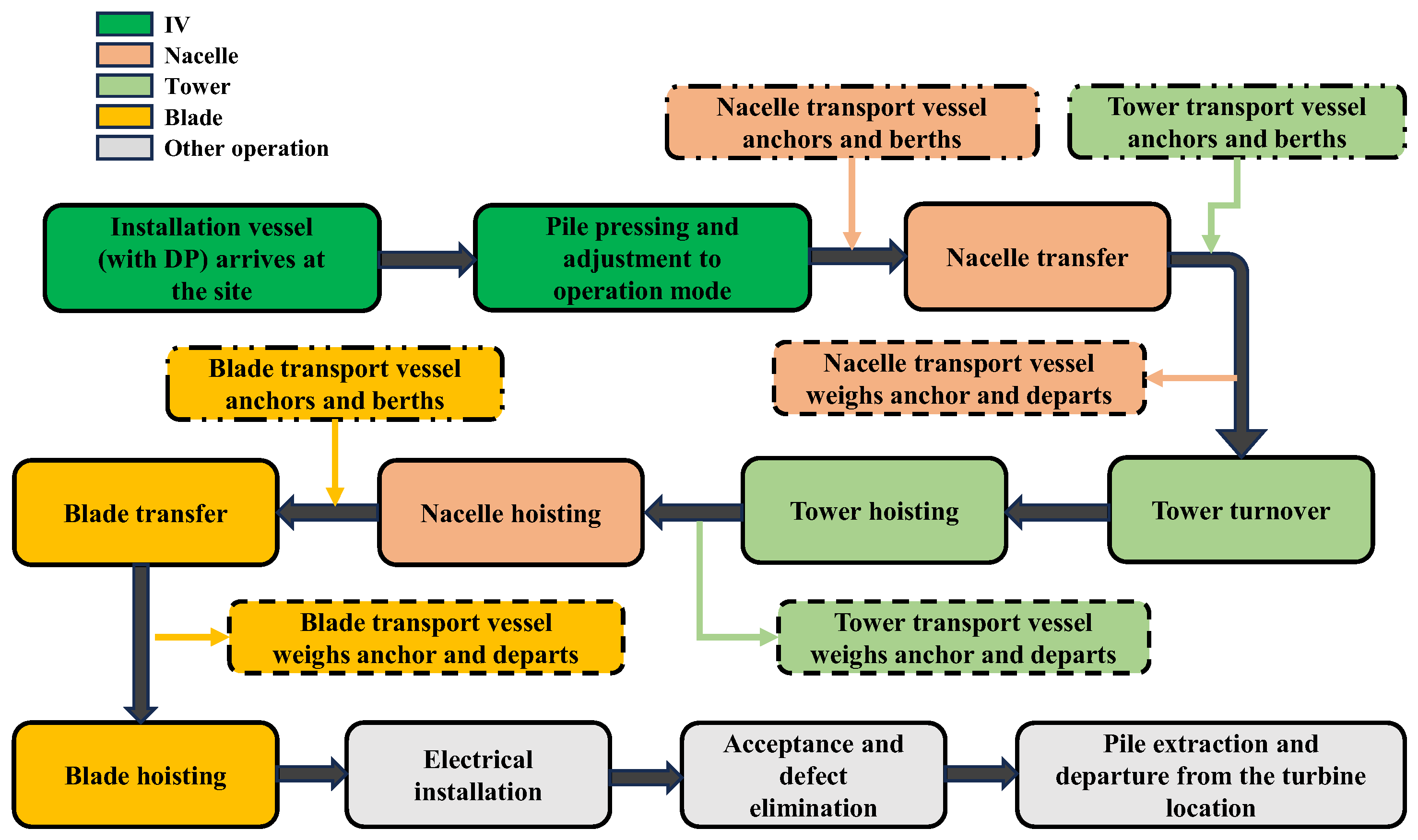
The installation process for a single turbine follows the sequence illustrated in Figure 1. First, the WTIV navigates to the designated installation site, uses its Dynamic Positioning (DP) system for precise positioning, and jacks up to create a stable working platform. Next, a sequence of feeder operations begins as TVs dock alongside the WTIV. Upon the arrival of the nacelle TV, the WTIV crane transfers the nacelle to a temporary deck storage position. After the nacelle TV departs, the tower TV moors alongside. The crane then lifts and installs the tower segments sequentially, performing auxiliary tasks in parallel. Once the tower installation is complete, the crane mounts the pre-stored nacelle onto the tower. Concurrently, the blade TV arrives, and the blades are transferred and installed using a specialized gripper. Finally, after the blade TV departs and the electrical commissioning and inspections are passed, the WTIV lowers its legs and proceeds to the next location.

From this detailed operational workflow, the core installation process is distilled into five key schedulable activities, which serve as the foundation of the optimization model. The sequence of tasks to be completed is as follows: (1) nacelle transfer, (2) tower installation, (3) nacelle installation, (4) blade transfer, and (5) blade installation.

3.2. Mathematical Model

Based on the description above, we define the OWT installation model as follows: Sets and Indices.

$\mathcal{T}$: Set of wind turbines to be installed, $t\in \mathcal{T}=\left\{N_1,\dots ,N_T\right\}$.

${\mathcal{T}}_0$: Set of all nodes including turbines and the port (base), $i,i^{\prime }\in {\mathcal{T}}_0=\mathcal{T}\cup \left\{0\right\}$.

${\mathcal{V}}_I$: Set of IVs, $v\in {\mathcal{V}}_I$.

${\mathcal{V}}_T$: Set of TVs, $u\in {\mathcal{V}}_T$.

$\mathcal{K}$: Set of wind turbine component types, $k\in \mathcal{K}=\left\{1\left(\mathrm{tower}\right), 2\left(\mathrm{nacelle}\right), 3\left(\mathrm{blade}\right)\right\}$.

$\mathcal{P}$: Set of operational phases for an IV at a single turbine, $p\in \mathcal{P}=\left\{1,2,3,4,5,6,7\right\}$, where 1—Sailing, 2—Jacking-up, 3—Nacelle transfer, 4—Tower installation, 5—Nacelle installation, 6—Blade installation, 7—Jacking-down.

$\mathcal{J}$: Set of all transport tasks generated from the installation plan, $j\in \mathcal{J}$.

${\mathcal{O}}_j$: Sequence of operational phases for a transport task $j$, $o\in {\mathcal{O}}_j=\left\{1, 2, 3, 4\right\}$, where 1—Loading, 2—Sailing, 3—On-site operation, 4—Return sailing.

$\mathcal{D}$: Set of days, $d\in \mathcal{D}$.

Parameters.

$C_v^I,C_u^T$: Daily charter costs for IV $v$ and TV $u$.

$S_v^I,S_u^T$: Sailing speeds of IV $v$ and TV $u$.

${\delta }_{i{i}^{\prime }}$: Sailing distance from node $i$ to node $i^{\prime }$.

$Q_k$: Number of sub-components for component type $k\in \mathcal{K}$ required per turbine.

$N_k$: Number of individual sub-components of type $k$ transferred in a single operation.

$D_k^i$: Installation time for a single sub-component of type $k$.

$D_k^t$: Transfer time for a single sub-component of type $k$.

$D_p$: Standard duration for operation $p\in \mathcal{P}$ that is independent of component quantity.

$D_k^l$: Loading time for a single sub-component of type $k$.

$t_j$: Target turbine location for task $j$.

$W_d\in \left\{1,0,-1\right\}$: Weather status on day $d$ (1: good; 0: moderate; −1: poor).

${\Omega }_{pw}\in \left\{0,1\right\}$: Binary parameter; equals 1 if installation operation $p$ is permitted under weather status $w$, and 0 otherwise.

$M$: A sufficiently large positive number.

Decision Variables.

$x_{vt}\in \left\{0,1\right\}$: 1 if turbine $t$ is assigned to IV $v$; 0 otherwise.

$y_{vi{i}^{\prime }}\in \left\{0,1\right\}$: 1 if IV $v$ travels from node $i$ directly to node $i^{\prime }$; 0 otherwise.

$z_{uj}\in \left\{0,1\right\}$: 1 if transport task $j$ is assigned to TV $u$; 0 otherwise.

${\tau }_{vtp}^s,{\tau }_{vtp}^e$: Start and end times for operation $p$ performed by IV $v$ at turbine $t$.

${\theta }_{ujo}^s,{\theta }_{ujo}^e$: Start and end times for operational phase $o$ of task $j$ performed by TV $u$.

$R_v^s,R_v^e$: Start and end times of the charter period for IV $v$.

$R_{uj}^s,R_{uj}^e$: Start and end times of the time window occupied by TV $u$ for task $j$.

${\sigma }_t\in \left\{0,1\right\}$: 1 if the blade installation for turbine $t$ is skipped (postponed); 0 otherwise.

${\chi }_{u,j_1,j_2}\in \left\{0,1\right\}$: 1 if transport task $j_1$ is performed immediately before task $j_2$ by TV $u$; 0 otherwise.

The primary objective is to minimize total installation costs. Since vessel charter rates are significant, this is equivalent to minimizing the total charter duration and eliminating redundant idle time between processes. The model’s formulation is as follows:

$$Z:min {\displaystyle \sum }_{v\in {\mathcal{V}}_I}{C}_v^I·({\displaystyle \lfloor }{\displaystyle \frac{R_v^e}{24}}{\displaystyle \rfloor }-{\displaystyle \lfloor }{\displaystyle \frac{R_v^s}{24}}{\displaystyle \rfloor }+1)+{\displaystyle \sum }_{u\in {\mathcal{V}}_T}{C}_u^T·(\lfloor {\displaystyle \frac{{\mathit{max}}_{j\left|z_{uj}=1\right.}{R}_{uj}^e}{24}}\rfloor -\lfloor {\displaystyle \frac{{\mathit{min}}_{j\left|z_{uj}=1\right.}{R}_{uj}^s}{24}}\rfloor +1)$$

(1)

Subject to following constraints:

$${\displaystyle \sum }_{v\in {\mathcal{V}}_I}{x}_{vt}=1, \forall t\in \mathcal{T}$$

(2)

$${\displaystyle \sum }_{i^{\prime }\in {\mathcal{T}}_0,i^{\prime }\ne i}{y}_{vi{i}^{\prime }}=x_{vi}, \forall v\in {\mathcal{V}}_I,i\in \mathcal{T}$$

(3)

$${\tau }_{vt{p}_k}^e\ge {\tau }_{vt{p}_k}^s+Q_k·D_k^i·x_{vt}, \forall v,t,p_k\in \left\{4,5,6\right\}$$

(4)

$${\tau }_{v,t,3}^e\ge {\tau }_{v,t,3}^s+N_2·D_2^i·x_{vt}, \forall v,t$$

(5)

$${\tau }_{vtp}^e\ge {\tau }_{vtp}^s+D_p·x_{vt}, \forall v,t,p\in \left\{1,2,7\right\}$$

(6)

$${\tau }_{v,t^{\prime },1}^s\ge {\tau }_{v,t,7}^e+{\displaystyle \frac{{\delta }_{t{t}^{\prime }}}{S_v^I}}-M\left(1-y_{vt{t}^{\prime }}\right), \forall v,t,t^{\prime }\in \mathcal{T}$$

(7)

$${\Omega }_{p,w_d}=1,\forall d\in \left[{\displaystyle \lfloor \frac{{\tau }_{vtp}^s}{24}\rfloor },{\displaystyle \lceil \frac{{\tau }_{vtp}^e}{24}\rceil }\right], \forall v,t,p$$

(8)

$${\Omega }_{p,-1}=0, \forall p\in \mathcal{P}$$

(9)

$${\Omega }_{6,0}=0$$

(10)

$${\displaystyle \sum }_{d=\lfloor {\tau }_{v,t,6}^s/24\rfloor }^{\lceil {\tau }_{v,t,6}^e/24\rceil }\left(1-{\Omega }_{6,W_d}\right)\le M·{\sigma }_t,\forall v\in {\mathcal{V}}_I,t\in \mathcal{T}$$

(11)

$${\tau }_{v,t^{\prime },6}^s\ge {\tau }_{v,t,7}^e-M·\left(1-{\sigma }_{t^{\prime }}\right),\forall v\in {\mathcal{V}}_I,t^{\prime }\in \mathcal{T},t\in \mathcal{T}\backslash \left\{t^{\prime }\right\}$$

(12)

$${\theta }_{u,j,2}^s\ge {\theta }_{u,j,1}^e$$

(13)

$${\theta }_{u,j,3}^s\ge {\theta }_{u,j,2}^e$$

(14)

$${\theta }_{u,j,4}^s\ge {\theta }_{u,j,3}^e$$

(15)

$${\theta }_{u,j,1}^e-{\theta }_{u,j,1}^s\ge Q_k·D_k^l·z_{uj}, \forall u,j,k\in \left\{1,3\right\}$$

(16)

$${\theta }_{u,j,1}^e-{\theta }_{u,j,1}^s\ge N_2·D_2^l·z_{uj}, \forall u,j$$

(17)

$${\theta }_{u,j,2}^e-{\theta }_{u,j,2}^s\ge {\displaystyle \frac{{\delta }_{0,t_j}}{S_u^T}}·z_{uj}, \forall u,j$$

(18)

$${\theta }_{u,j,4}^e-{\theta }_{u,j,4}^s\ge {\displaystyle \frac{{\delta }_{t_j,0}}{S_u^T}}·z_{uj}, \forall u,j$$

(19)

$${\theta }_{u,j,3}^s\le {\tau }_{v,t_j,p_j}^s+M\left(1-z_{uj}\right)$$

(20)

$${\theta }_{u,j,3}^e\ge {\tau }_{v,t_j,p_j}^e-M\left(1-z_{uj}\right)$$

(21)

$${\theta }_{u,j_2,1}^s\ge {\theta }_{u,j_1,4}^e-M\left(1-{\chi }_{u,j_1,j_2}\right), \forall u,j_1\ne j_2 \mathrm{with} z_{u{j}_1}=1,z_{u{j}_2}=1$$

(22)

$$R_v^s\le {\tau }_{v,t,1}^s-{\displaystyle \frac{{\delta }_{0t}}{S_v^I}}+M\left(1-y_{v0t}\right), \forall t\in \mathcal{T}$$

(23)

$$R_v^e\ge {\tau }_{v,t,7}^e+{\displaystyle \frac{{\delta }_{t0}}{S_v^I}}-M\left(1-y_{vt0}\right), \forall t\in \mathcal{T}$$

(24)

$$R_{uj}^s={\theta }_{u,j,1}^s, R_{uj}^e={\theta }_{u,j,4}^e, \forall u,j$$

(25)

$${\tau }_{vtp}^s,{\theta }_{ujo}^s,R_v^s,R_{uj}^s\ge 0$$

(26)

Table 1. Summary of mathematical constraints and corresponding physical interpretations.

Constraint	Category	Physical Interpretation and Function
(2) and (3)	Routing	Assignment and Flow: Guarantees each turbine is served by exactly one IV and maintains route continuity.
(4)–(7)	Scheduling	IV Operation Timing: Links operational phases; ensures start times account for duration and travel time.
(8)–(12)	Weather	Environmental Limits: Aligns tasks with valid weather windows; enforces postponements for specific tasks (e.g., blades).
(13)–(19) and (22)	Logistics	TV Workflow: Defines the sequence: Loading → Sailing → On-site → Return, including duration limits and task sequencing.
(20)–(21)	Sync	Vessel Synchronization: Coordinates the handover/interaction time windows between IVs and TVs on-site.
(23)–(25)	Charter	Charter Period: Defines the exact start and end dates of vessel leases based on active tasks.
(26)	Variable	Domain: Defines binary and continuous decision variables.

summarizes the mathematical constraints (Equations (2)–(26)) and their physical interpretations to clarify the complex operational dependencies and fleet synchronization. Detailed mathematical descriptions and derivations can be found in Appendix A.

The problem described above constitutes an MILP model. To assess the feasibility of exact methods, preliminary experiments were conducted using the commercial solver CPLEX on a standard workstation. While the solver successfully identified optimal solutions for small-scale instances (e.g., 5 turbines), it encountered significant challenges with real-world scale instances (55 turbines). Specifically, for the full-scale problem, the solver failed to converge to a feasible integer solution even after a runtime of 3 h, often terminating prematurely due to memory exhaustion. This intractability is consistent with findings by Irawan et al. [43], who reported that commercial solvers encountered out-of-memory errors and negligible optimality gap improvements when scheduling similar offshore decommissioning operations. Similarly, Amorosi et al. [20] also reported similar computational intractability due to model complexity.

Given that the present study involves not only vessel routing but also a tight coupling between installation and transport tasks (Equations (20) and (21), the computational burden exceeds that of standard routing problems. Unlike decomposable logistics problems, these synchronization constraints necessitate global adjustments across the heterogeneous fleet for any local schedule change. Consequently, direct attempts to solve real-world instances with general-purpose solvers are computationally prohibitive due to the exponential growth of the search space.

Regarding solution methodologies, alternative decomposition techniques were considered but deemed less viable for this specific context. While the benders decomposition was applied in related offshore studies (e.g., Ursavas [19]), its efficacy relies on separating the model into a master problem and computationally tractable sub-problems. In this model, the sub-problem remains highly complex due to weather-dependent time windows (Equations (8)–(10)), which introduce discontinuous availability constraints that impede the generation of efficient optimality cuts. Similarly, regarding the rolling horizon approach, although it could reduce computational load by segmenting the planning horizon, it risks compromising the global optimality of strategic decisions. Since minimizing the total charter cost is a strategic objective, a myopic rolling view may lead to suboptimal fleet commitment decisions.

In light of these computational barriers and the limitations of exact decomposition methods, this study adopts a metaheuristic approach. This method combines algorithmic search with domain-specific insights to solve the problem efficiently while ensuring operational realism.

4. Solution Approach

The multi-vessel collaborative scheduling problem can be decomposed into two subproblems. First, the initial scheduling phase focuses on allocating tasks across multiple vessels and planning routes to balance workloads. Second, the optimization phase determines the optimal schedule under real-time demand, where the operations of IVs and TVs mutually influence one another.

4.1. Initial Scheduling Solution

Because weather is inherently uncertain, directly incorporating it complicates model validation. Therefore, this study first focuses on a scenario with ideal weather conditions to establish a baseline solution method. Subsequently, the actual weather conditions are incorporated as an input into the original scheduling model for solving.

The preliminary vessel scheduling plan was supplied by industrial partners and features a core configuration in which each IV is paired with a dedicated fleet of TVs (one each for towers, nacelles, and blades), forming $m$ independent operational teams.

This configuration is subject to two fundamental constraints: Firstly, as outlined in the charter agreements, vessels may only be continuously chartered for a single cycle and cannot be redeployed during periods of inactivity. Secondly, each operational team is solely responsible for its assigned turbine units and is prohibited from performing tasks for other teams. In light of the aforementioned constraints, teams function in an autonomous manner, thereby reducing the complex scheduling problem to an MTSP with scheduling constraints. In this MTSP formulation, the m operational teams act as the m “salesmen,” the locations of the turbines to be installed are the “cities,” and the port serves as the common origin and destination for all salesmen. Unlike the classic MTSP objective of minimizing total path length, the primary goal here is to minimize installation costs while preventing excessive task assignment to any single vessel. Therefore, the problem aims to minimize the longest tour among all teams. This approach ensures a balanced workload distribution and prevents an overloaded schedule for a single team from delaying the entire project.

The MTSP is NP-hard; thus, heuristics and metaheuristics are the predominant approaches for practical, large-scale instances. A strategy that has been proven to be successful and adopted by a wide range of users is the “cluster-first, route-second” paradigm. For example, Peng et al. [44] integrated K-means clustering with a genetic algorithm, while Baydogmus [45] employed a parallel K-means and elitist ant colony optimization. The methodology employed involves the initial partitioning of the nodes (cities) into clusters, followed by the resolution of a standard Traveling Salesman Problem (TSP) for each cluster. An alternative to geometric clustering is criteria-based assignment. Ergüven et al. [46] proposed a relative distance method that assigns cities to salesmen based on a composite cost coefficient, balancing global cost, local cost, and workload. The extant literature provides a robust foundation for decomposition-based approaches to the MTSP.

Drawing on this conceptual paradigm, this paper proposes a tailored three-stage heuristic algorithm designed to generate high-quality, engineering-feasible solutions for the OWF installation problem. The problem can be formally stated as follows:

As outlined in Section 3.2, let $\mathcal{T}=\left\{N_1,N_2,\dots ,N_T\right\}$ denote the set of turbines awaiting installation and ${\mathcal{V}}_I=\left\{v_1,v_2,\dots ,v_m\right\}$ represent the set of $m$ IV teams. The core objective is to identify a partition of the turbine set, denoted as $P=\left\{{\mathcal{T}}_1,{\mathcal{T}}_2,\dots ,{\mathcal{T}}_m\right\}$, alongside a corresponding installation tour ${\tau }_i$ for each vessel team $v_i$ to cover its assigned turbine subset ${\mathcal{T}}_i$. The overarching objective is to minimize the maximum completion time across all vessel teams.

The proposed heuristic algorithm comprises three sequential stages:

Stage 1. Initial Partitioning via Balanced Sweep Clustering.

This stage generates an initial partition $P^{\left(0\right)}=\left\{{\mathcal{T}}_1^{\left(0\right)},{\mathcal{T}}_2^{\left(0\right)},\dots ,{\mathcal{T}}_m^{\left(0\right)}\right\}$ using a port-centered sweep clustering algorithm. The algorithm groups turbines according to their angular positions relative to the port, thereby forming geometrically coherent clusters. This preliminary grouping is then refined via a local search procedure, which balances the workload across clusters by accounting for both the number of turbines and their spatial distribution within each subset.

Stage 2. Intra-Cluster Route Optimization.

Following the finalization of the initial partition, the MTSP inherent to the scheduling task is decomposed into $m$ independent TSP instances, with one instance allocated for each turbine cluster. For each turbine cluster ${\mathcal{T}}_i$, a high-quality installation tour ${\tau }_i$ is constructed through a two-step process: firstly, the computationally efficient nearest neighbor heuristic is applied to rapidly generate an initial tour ${\tau }_i^{\left(init\right)}$. Then the 2-opt algorithm is iteratively implemented on this initial tour to eliminate path crossings and other suboptimal route structures, thereby yielding a significantly optimized tour ${\tau }_i$.

Stage 3. Global Refinement via Penalized Local Search.

The objective of this final stage is to further refine the global solution through the iterative reallocation of individual turbines between clusters. A local search mechanism explores the solution space by executing move operations, whereby a single turbine $t$ is transferred from its original cluster ${\mathcal{T}}_i$ to a neighboring cluster ${\mathcal{T}}_j$. The acceptance of each move is determined by its impact on the maximum completion time objective, with a penalty function incorporated to deter excessive workload imbalances across clusters. The iteration is continued until a predefined stopping criterion is satisfied, yielding a final solution with favorable comprehensive cost performance. The pseudo-code for the algorithm is provided in full in Algorithm A1.

The routes for all IVs are determined on the basis of the preceding results. Next, the installation schedule is established following the procedure in Figure 1. Given that the configuration of the TVs is fixed and sufficient for all logistical requirements, their schedule is directly derived from that of the IVs.

4.2. Scheduling Optimization

Based on the baseline installation schedule derived from the preceding analysis, an ideal timeline for all IVs is established. Within this timeline, each operational step requiring external material supply corresponds to a specific transport task with a defined deadline. To solve the complex assignment and scheduling problem for these transport tasks, this paper proposes a two-stage solution strategy. This strategy first generates a high-quality feasible solution using a computationally efficient heuristic, which then serves as the initial state for a metaheuristic optimization algorithm to find a globally optimal or near-optimal solution.

Stage 1. Initial schedule and fleet sizing via an EDF-based greedy heuristic.

To rapidly generate a feasible initial schedule, a greedy heuristic based on the EDF principle is employed. Since the number of vessels is unknown, this algorithm dynamically adds vessels to the fleet as needed. The objective at each step is strictly to meet the task’s deadline at the earliest possible time.

The full implementation procedure is detailed in Algorithm A2. Tasks are first sorted by their respective deadlines, after which the algorithm cycles through each task in this ordered sequence. For every task, the algorithm assesses two deployment options: either assigning the task to an existing vessel in the current fleet, specifically the one capable of completing the work at the earliest possible time, or allocating it to a newly chartered vessel that is presumed to be available on demand.

The algorithm greedily chooses the option that will result in the earlier completion time. If chartering a new vessel is deemed to be the superior local choice, a new vessel is added to the fleet. This heuristic effectively determines an initial fleet size and schedule. However, its myopic nature frequently results in an over-provisioning of vessels, as it may add a new vessel for a minor timing advantage without considering the significant charter cost. This renders the resulting schedule an optimal candidate for further optimization.

Stage 2. Schedule optimization via SA.

To surmount the local optimality limitation of the greedy heuristic, a more sophisticated metaheuristic optimization is required. The schedule generated by the EDF algorithm serves as a high-quality initial solution for an SA optimization phase. While genetic algorithms were initially evaluated as a potential alternative, they delivered suboptimal performance given the unique structure of this scheduling problem. Following a rigorous evaluation of available options, SA was selected because it is highly suited to discrete combinatorial optimization problems such as task allocation. Specifically, SA does not require the solution space to be continuous or differentiable. The efficacy of this metaheuristic in handling complex constraints has been validated in related optimization fields. For instance, Yoon et al. [47] demonstrated the effectiveness of SA in solving a location routing problem under strict operational constraints. Although their work focused on urban infrastructure, the success of their methodology in refining heuristic solutions is highly relevant to the maritime scheduling logic adopted here.

The fundamental objective of the SA algorithm is to iteratively refine the initial schedule through intelligent exploration of the solution neighborhood. The objective is to achieve an optimal balance between minimizing the number of TVs deployed and eliminating unnecessary waiting times for IVs. This is to be accomplished through systematic reallocation and swapping of transport tasks. In this search process, a composite cost function is employed to guide the search process, enabling a quantitative assessment to be made. Notably, this function does not correspond to the actual total project cost; instead, it is a carefully designed objective function tailored specifically for this optimization task:

$$Z_{SA}=C_{tranport\_proxy}+C_{wait}+C_{penalty}$$

(27)

where $C_{tranport\_proxy}$ represents the TV charter cost, $C_{wait}$ represents the penalty for IV waiting time, and $C_{penalty}$ represents the penalty for the number of TVs.

$$C_{transport\_proxy}={\displaystyle \sum }_{u\in {\mathcal{V}}_T}{C}_u^T·\left({\displaystyle \lfloor \frac{{\mathit{max}}_{j\left|z_{uj}=1\right.}{R}_{uj}^e}{24}\rfloor }-{\displaystyle \lfloor \frac{{\mathit{min}}_{j\left|z_{uj}=1\right.}{R}_{uj}^s}{24}\rfloor }+1\right)$$

(28)

$$C_{wait}={\displaystyle \sum }_{u\in {\mathcal{V}}_T}{\displaystyle \frac{C_v^I}{24}}·\mathit{max}(0,{\theta }_{u,j,3}^s-{\tau }_{v\left(j\right),t_j,p_j}^s)$$

(29)

$$C_{penalty}=C_u^T·{\displaystyle \sum }_{u\in {\mathcal{V}}_T}{y}_u$$

(30)

$${\displaystyle \sum }_{j\in J}{z}_{uj}\le M·y_u, \forall u\in {\mathcal{V}}_T$$

(31)

The SA optimization process is delineated in Algorithm A3. Since neighborhood solutions in SA are generated stochastically, the algorithm is executed multiple times to mitigate the risk of converging to a local optimum and to increase the probability of discovering a globally superior solution.

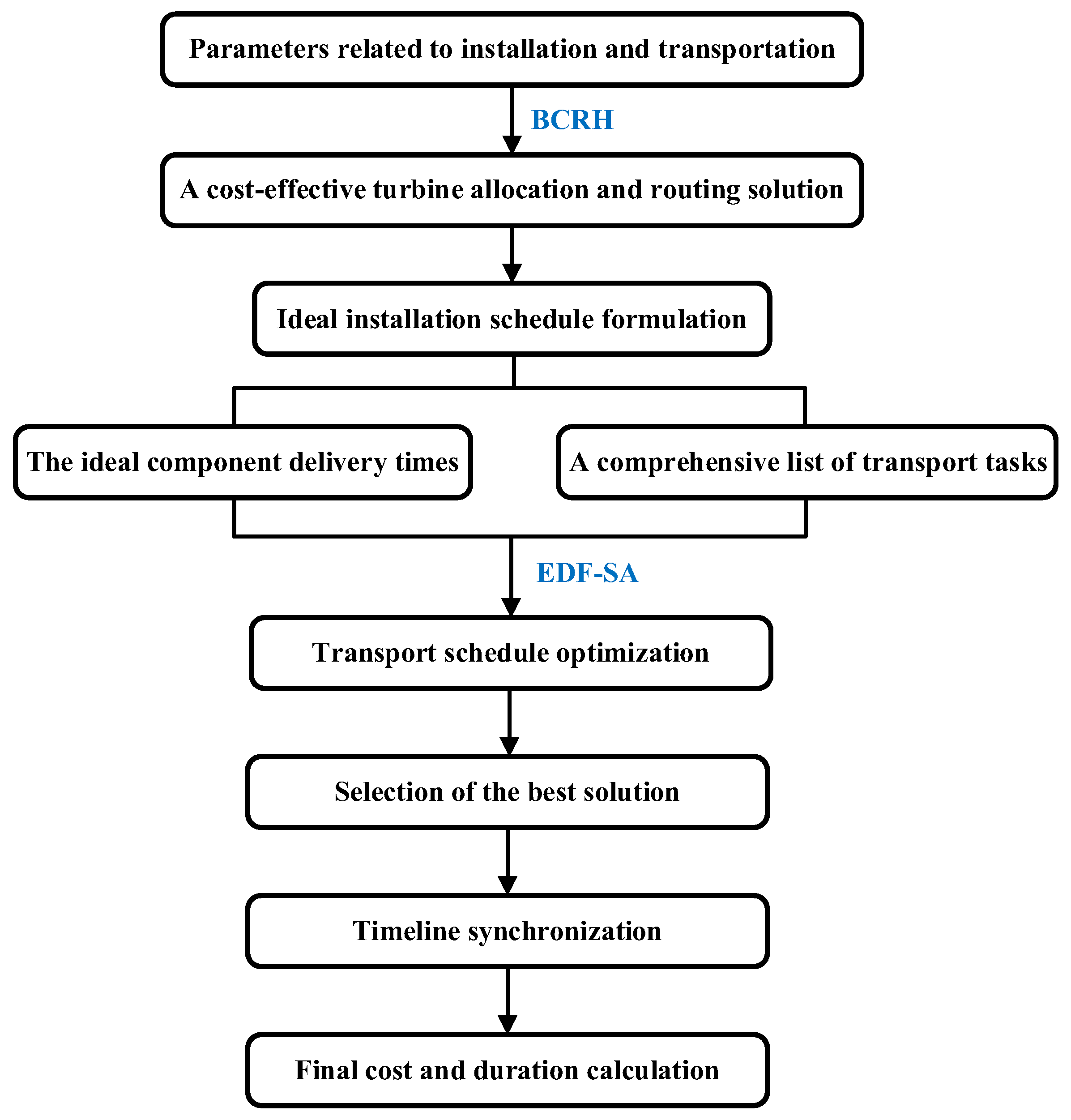
The complete methodology for solving the OWF installation scheduling problem under deterministic conditions is illustrated in Figure 2 and structured into three main stages:

Stage 1. Core scheduling and optimization. This preliminary stage comprises the iterative modeling and solution process, which incorporates three fundamental components: (a) assigning turbines to vessels and optimizing routing, (b) formulating a baseline installation schedule, and (c) developing the transport schedule using the EDF-SA hybrid approach.

Stage 2. Global search via multiple independent runs. To guarantee the derivation of a high-quality global solution, the entire Stage 1 procedure is executed multiple times independently. The solution that exhibits the global minimum cost across all iterations is designated as the final candidate.

Stage 3. Final schedule construction and performance evaluation. The optimal solution identified in Stage 2 is utilized to reconstruct a detailed project timeline and generate the final vessel scheduling Gantt chart. This Gantt chart facilitates precise calculation of the project’s ultimate total cost and overall completion time.

5. Computational Experiments

5.1. Case Study Configuration and Initial Scheduling Analysis

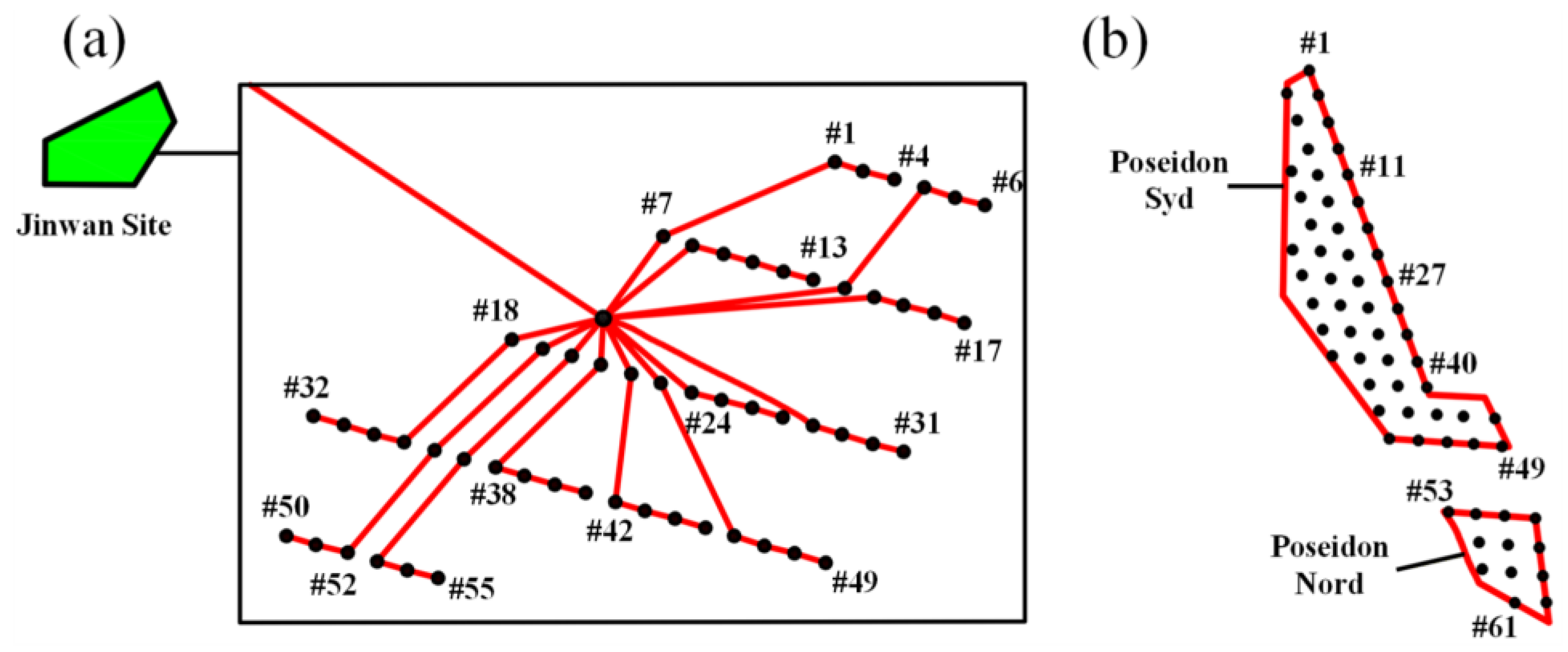
This study appraises and optimizes vessel strategies for two discrete OWF installation projects: the 55-turbine Zhuhai Jinwan Wind Farm (Wind Farm 1) and the 61-turbine Swedish Poseidon Wind Farm (Wind Farm 2). The two projects are illustrated in Figure 3, and the specific center coordinates for the turbines in Wind Farm 1 are detailed in

Table A1. Center coordinates of wind turbines at the Zhuhai Jinwan Wind Farm (CGCS2000).

Turbine ID	Latitude (N)	Longitude (E)	Turbine ID	Latitude (N)	Longitude (E)
#1	21°56′05.583″	113°27′53.926″	#29	21°53′43.521″	113°27′58.665″
#2	21°56′01.045″	113°27′53.926″	#30	21°53′38.979″	113°28′14.659″
#3	21°55′56.532″	113°28′26.039″	#31	21°53′34.471″	113°28′30.738″
#4	21°55′51.974″	113°28′42.395″	#32	21°53′53.649″	113°23′16.413″
#5	21°55′47.433″	113°28′58.451″	#33	21°53′49.147″	113°23′32.482″
#6	21°55′42.910″	113°29′14.526″	#34	21°53′44.629″	113°23′48.525″
#7	21°55′27.021″	113°26′22.767″	#35	21°53′40.080″	113°24′04.556″
#8	21°55′22.509″	113°26′38.819″	#36	21°53′35.584″	113°24′20.592″
#9	21°55′17.980″	113°26′54.895″	#37	21°53′31.057″	113°24′36.633″
#10	21°55′13.433″	113°27′10.931″	#38	21°53′26.549″	113°24′53.031″
#11	21°55′08.919″	113°27′26.997″	#39	21°53′22.020″	113°25′09.074″
#12	21°55′04.379″	113°27′43.021″	#40	21°53′17.498″	113°25′25.148″
#13	21°54′59.833″	113°27′59.422″	#41	21°53′12.970″	113°25′41.156″
#14	21°54′55.34″	113°28′15.459″	#42	21°53′08.432″	113°25′57.225″
#15	21°54′50.780″	113°28′31.499″	#43	21°53′03.889″	113°26′13.234″
#16	21°54′46.274″	21°54′46.274″	#44	21°52′59.373″	113°26′29.278″
#17	21°54′41.778″	113°29′03.575″	#45	21°52′54.837″	113°26′45.354″
#18	21°54′33.321″	113°25′01.818″	#46	21°52′50.335″	113°27′01.342″
#19	21°54′28.796″	113°25′17.871″	#47	21°52′45.776″	113°27′17.411″
#20	21°54′24.265″	113°25′33.926″	#48	21°52′41.293″	113°27′33.459″
#21	21°54′19.734″	113°25′49.933″	#49	21°52′36.733″	113°27′49.465″
#22	21°54′15.220″	113°26′06.007″	#50	21°52′51.226″	113°23′01.697″
#23	21°54′10.697″	113°26′22.026″	#51	21°52′46.708″	113°23′17.744″
#24	21°54′06.132″	113°26′38.098″	#52	21°52′42.163″	113°23′33.816″
#25	21°54′01.644″	113°26′54.150″	#53	21°52′37.639″	113°23′49.869″
#26	21°53′57.135″	113°27′10.179″	#54	21°52′33.115″	113°24′05.908″
#27	21°53′52.592″	113°27′26.559″	#55	21°52′28.608″	113°24′21.903″
#28	21°53′48.059″	21°53′48.059″

. The configuration of the computational models was undertaken in accordance with the input data specified in

Table 2. Experimental input data.

Parameter	Value	Parameter	Value
$\left|{\mathcal{T}}_1\right|$	55	$Q_k$	4 ($k=1$), 1 ($k=2$), 3 ($k=3$)
$\left|{\mathcal{T}}_2\right|$	61	$N_k$	5 ($k=2$)
${\mathcal{V}}_I$	1/2/3/4	$D_k^i$	2 h ($k=1$), 4 h ($k=2$), 5 h ($k=3$)
$C_v^I$	$200,000	$D_k^t$	1.5 h ($k=2$)
$C_u^T$	$60,000	$D_p$	1.5 h ($p=2$), 1.5 h ($p=7$)
$S_v^I$	8 knot	$D_k^l$	1 h
$S_u^T$	12 knot

. To ensure simulation fidelity, parameter values such as charter costs and operational durations were derived from actual project data and expert consultation provided by our industrial partner, Guangzhou Bihai New Energy Co., Ltd. In addition, a maximum fleet size of four IVs was established, while the required number of TVs was treated as a decision variable to be optimized.

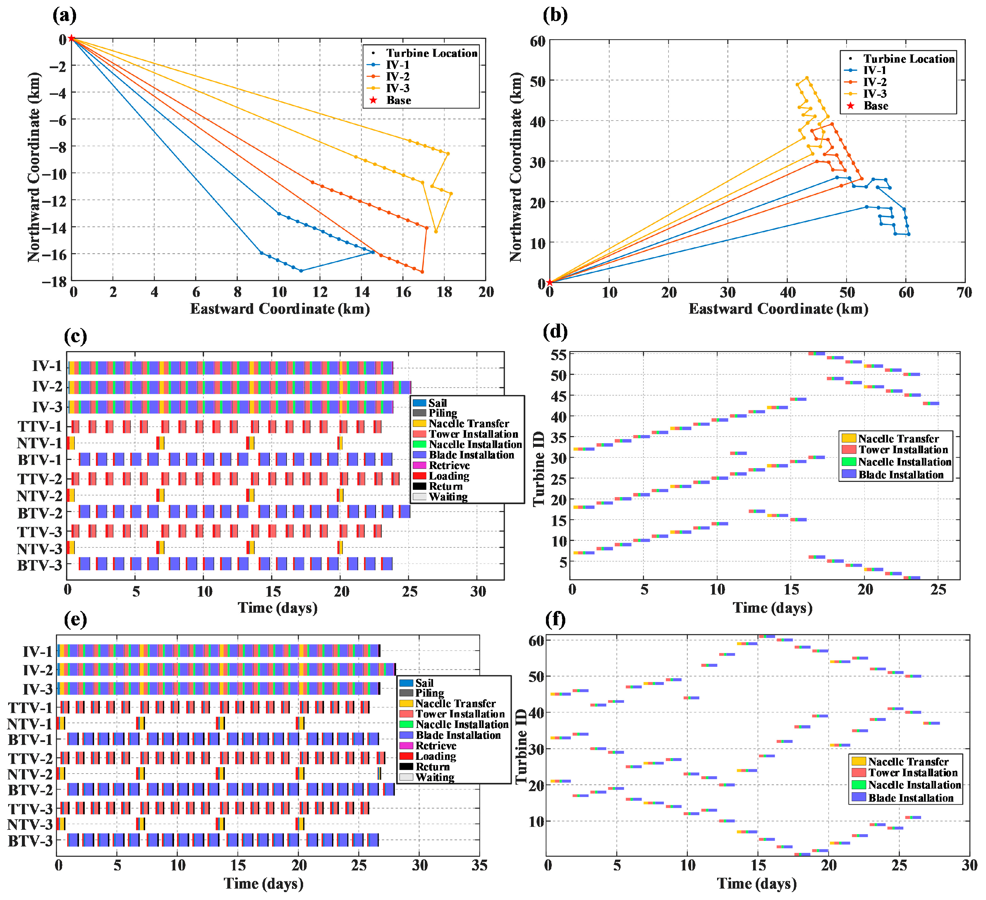
Utilizing a scenario comprising three IVs as a case study, the initial scheduling results generated from the aforementioned data are illustrated in Figure 4. Figure 4a,b illustrate the routes of the IVs for each wind farm, with all vessels departing from and returning to the port. The corresponding installation Gantt charts for Wind Farm 1 and Wind Farm 2 are presented in Figure 4c–f, respectively. The analysis demonstrates that the installation times for each IV were largely consistent across both wind farms, which aligns with expectations. However, the TVs exhibited significant idle time, indicating substantial potential for optimization in the vessel scheduling, particularly for the transport fleet.

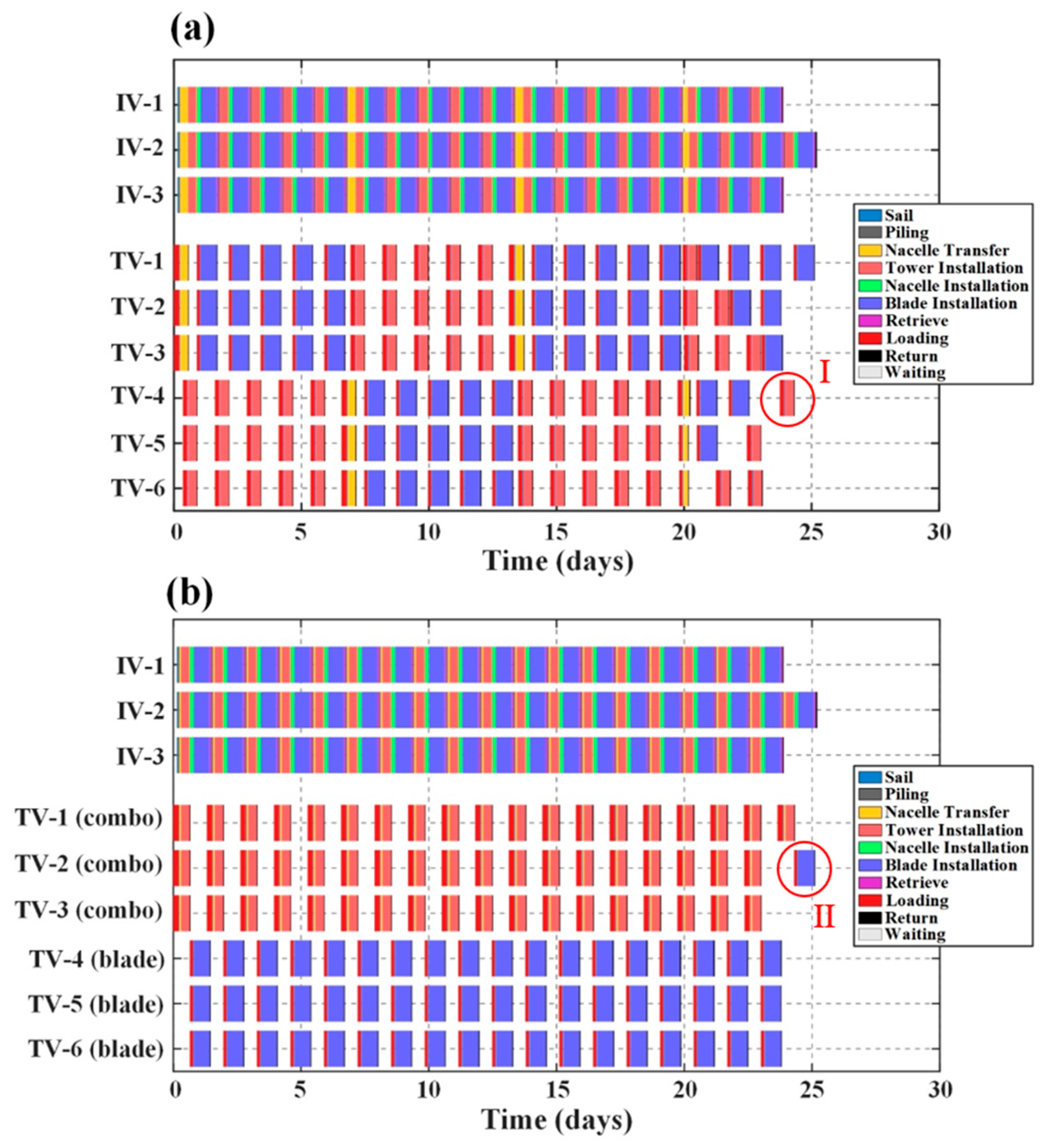
Drawing on this insight, the scheduling approach was further refined by decoupling the rigid TV-IV assignment schemes. Specifically, all transport tasks associated with each IV were extracted and centrally allocated to the TV fleet in accordance with the EDF principle. The resulting Gantt chart is displayed in Figure 5. For Wind Farm 1 under the component-wise transport model (see Figure 5a), this revised method reduced the required number of TVs from nine to six, with all transport tasks completed on schedule. It is important to note that, while this schedule has been optimized at a local level, it has not been identified as being globally optimal. For instance, the reallocation of task I to TV-5 would result in a further reduction in the overall vessel charter duration. A comparable suboptimal allocation, which is designated as allocation II, was also identified in the mixed-loading transport schedule (see Figure 5b). The result is a transport strategy that is elaborated upon in subsequent sections. The incorporation of the SA algorithm, as outlined in Section 3.2, is imperative in order to overcome the limitations imposed by local optimality. These findings thus validate the necessity of applying the SA algorithm to this scheduling problem.

5.2. Algorithm Validation and Proxy Objective Verification

Before evaluating the final optimization results, it is necessary to strictly validate the competitiveness and robustness of the proposed EDF-SA approach. Thus, a comparative analysis was conducted against two baseline metaheuristics: a standard Genetic Algorithm (GA) and a Pure Simulated Annealing (Pure SA) algorithm initialized with random solutions. To ensure a fair comparison, the computational budget was standardized across all algorithms. Both GA and SA variants were restricted to approximately $2\times {10}^4$ objective function evaluations per run. The specific parameter settings for each algorithm are detailed in

Table 3. Detailed parameter specifications for EDF-SA, Pure-SA, and GA.

Algorithm	Parameter	Symbol	Value
EDF-SA/Pure SA	Initial temperature	$T_0$	200,000
	Final temperature	$T_f$	50
	Cooling rate	$\alpha$	0.96
	Iterations per temperature	$L_{iter}$	100
GA	Population size	$N_{pop}$	100
	Max generations	$G_{max}$	200
	Mutation rate	$P_m$	0.25
	Crossover rate	$P_c$	0.85

.

Table 4. Experimental results comparison between the proposed EDF-SA and baseline metaheuristics (Pure SA and GA).

Algorithm	IVs	TVs	Average Time (s)	Best Cost ($)	Average Cost ($)
EDF-SA	1	2	9.24	26,120,000	26,120,000
	2	4	9.22	26,180,000	26,183,000
	3	6	9.65	26,320,000	26,350,000
	4	8	10.95	26,780,000	26,800,000
Pure SA	1	2	10.55	26,180,000	26,240,000
	2	4	11.75	26,380,000	26,440,000
	3	6	12.61	26,440,000	26,495,000
	4	8	13.83	27,020,000	27,320,000
GA	1	2	30.47	26,120,000	26,180,000
	2	4	44.53	26,240,000	26,260,000
	3	6	48.16	26,380,000	26,406,000
	4	8	56.72	27,020,000	27,082,000

summarizes the comparative results averaging over 20 independent runs for each scenario. Notably, this analysis focuses specifically on Wind Farm 2 (Scheme 3). Scheme 3 represents EDF-SA for component-wise transport, and the remaining schemes will be described subsequently. The average time metric in the table represents the pure algorithmic solving duration and excludes overheads such as data visualization. The data reveals that the EDF-SA algorithm achieves an optimal trade-off between solution quality and computational efficiency. Pure SA exhibits a marked discrepancy between the best and average costs, which suggests instability and a strong dependence on initial random seeds. Conversely, the EDF-SA method consistently converges with high-quality solutions with negligible deviation. Moreover, while the GA yields competitive solutions, it is computationally expensive, requiring 3–5 times the solving duration of EDF-SA. These findings confirm that EDF initialization significantly improves SA’s search capability.

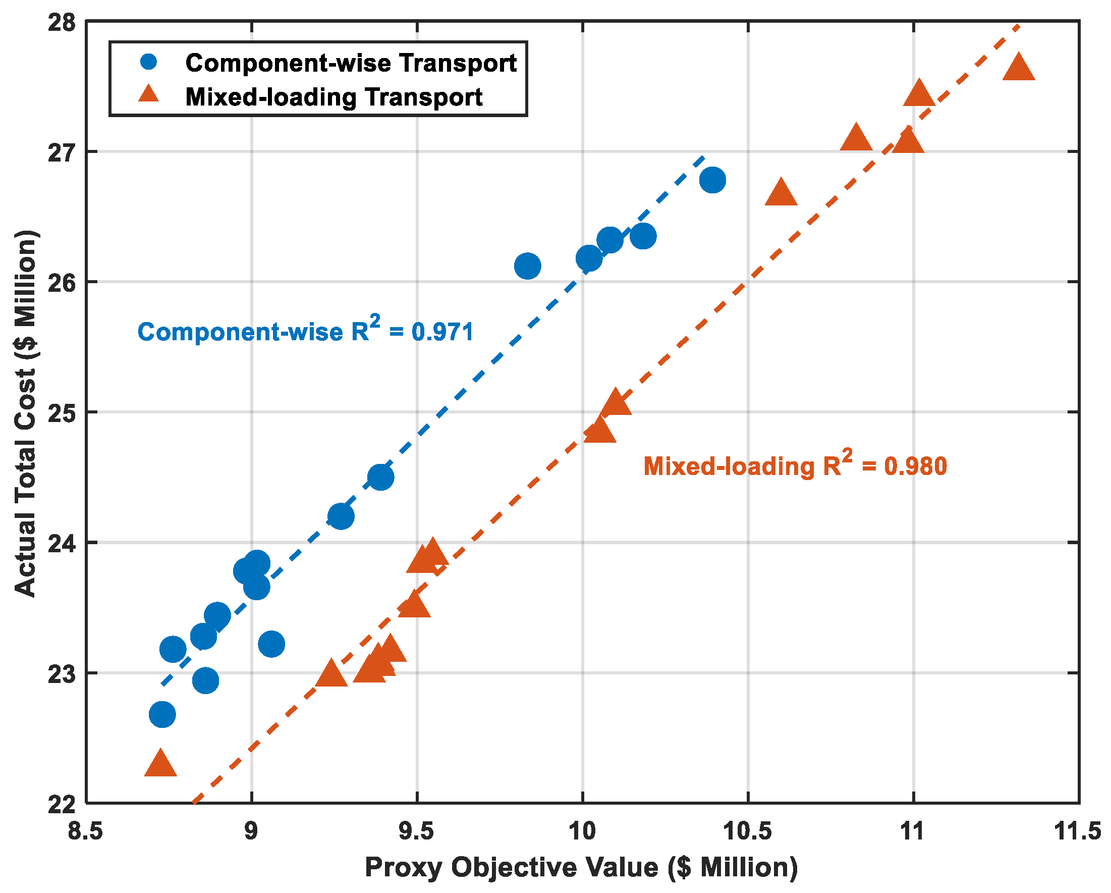
Furthermore, the reliability of the proxy objective function ($Z_{SA}$) was verified through correlation analysis. As illustrated in Figure 6, the results reveal a significant positive linear correlation between the proxy objective and real-world financial cost. Specifically, the coefficient of determination ($R^2$) reaches 0.971 for the component-wise transport strategy and 0.980 for the mixed-loading transport strategy. Such high $R^2$ values indicate that the proxy function $Z_{SA}$ successfully captures over 97% of the variance in the actual cost structure, confirming its reliability as an optimization guide. It is noteworthy that the two strategies align along distinct, nearly parallel regression lines. This offset reflects the inherent structural difference in baseline costs. However, the strict linearity observed in both scenarios demonstrates that the proxy function accurately tracks the marginal variations in total costs regardless of the baseline. This confirms that minimizing $Z_{SA}$ effectively drives the solution toward the economic optimum, thereby validating its effectiveness and robustness as a generalized optimization objective.

5.3. Optimization Results and Analysis

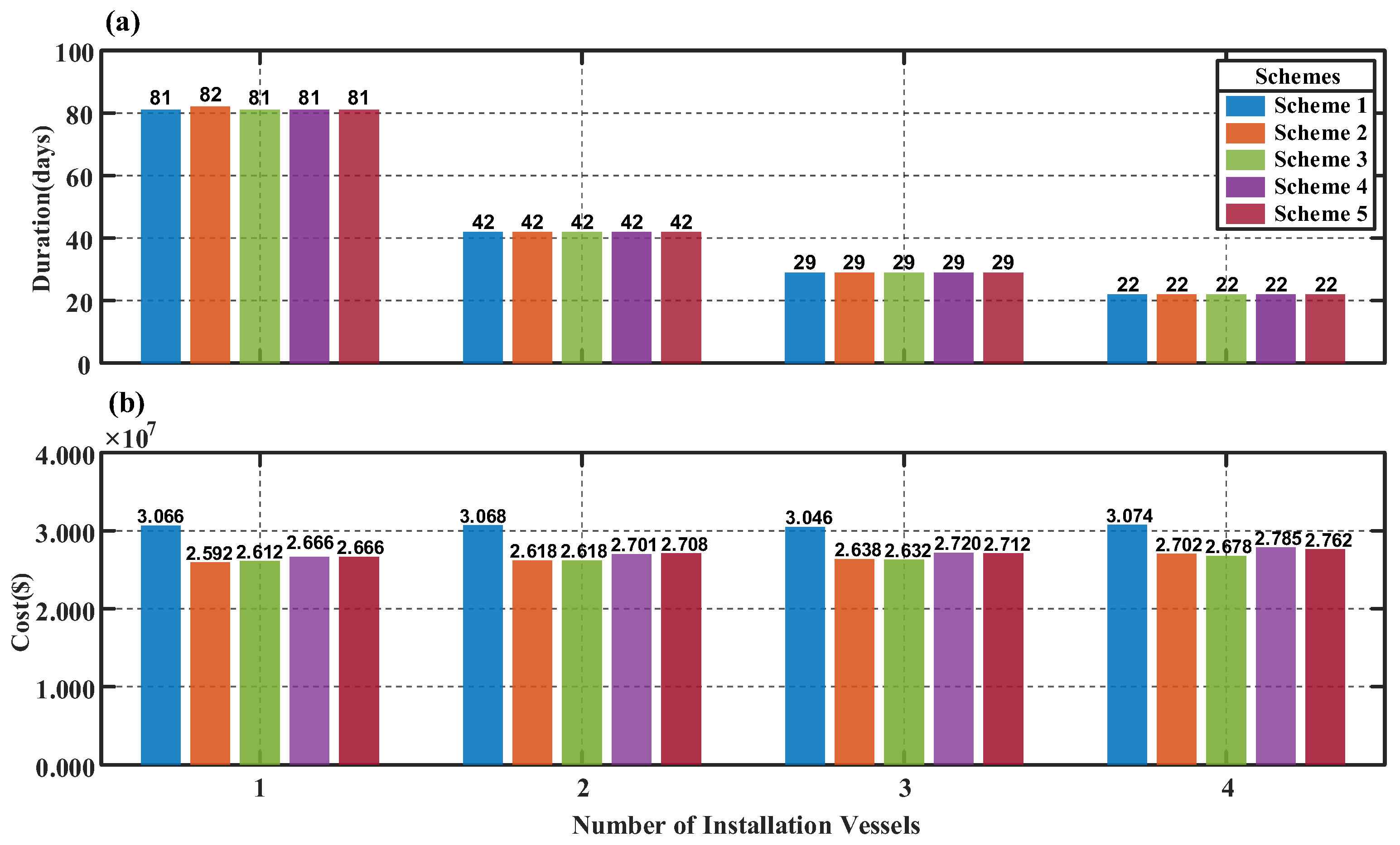
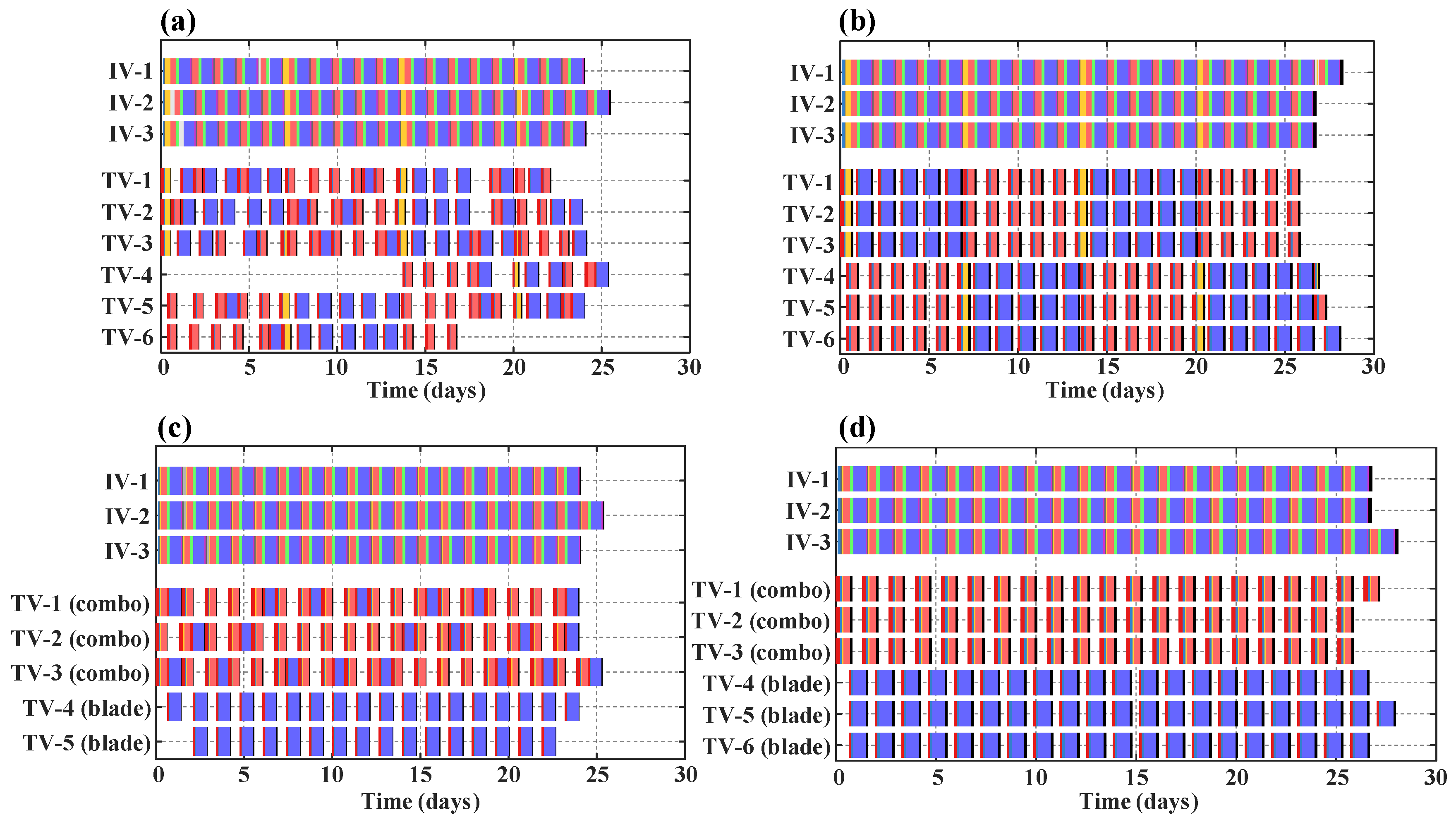
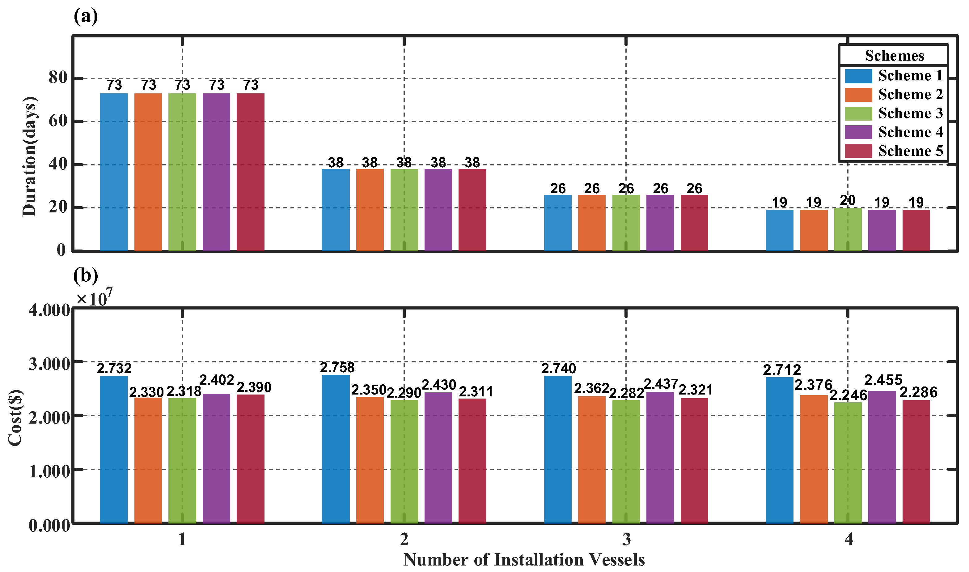
To pursue a global optimum, an EDF-SA hybrid approach was employed. The scheduling Gantt charts calculated for Wind Farm 1 and Wind Farm 2 with this method are shown in Figure 7a,b, with a legend consistent with Figure 5. The strategic placement of waiting times within the charts is intended to achieve an effective balance between the cost of augmenting the number of TVs and the duration of the project. Due to the capacity limitations of TVs, the industry standard is the separate transport of nacelles, towers, or blades. However, a mixed-loading approach, especially for nacelles and towers, has the potential to yield a lower-cost scheduling plan. To investigate this, a mixed-loading TV was defined. Following consultations with industry experts, the daily charter rate, $C_u^T$, was set to USD 70,000. After modifying the corresponding installation logic, the calculation of the mixed-loading scenario was conducted. The following five schemes were evaluated: Scheme 1 (initial plan), Scheme 2 (EDF-only for component-wise transport), Scheme 3 (EDF-SA for component-wise transport), Scheme 4 (EDF-only for mixed-loading), and Scheme 5 (EDF-SA for mixed-loading). As illustrated in Figure 7c,d, the Gantt charts for Wind Farm 1 and Wind Farm 2 utilize the mixed-loading approach. It is noteworthy that the optimized schedule for Wind Farm 2 (Figure 7d) coincides precisely with the more optimal schedule referenced in the context of Figure 5b.

A thorough examination of Figure 8 and Figure 9 indicates that the cost of installation of both wind farms exhibits fluctuations in relation to the number of IVs, while the duration of the installation process demonstrates a consistent decline. For Wind Farm 1, the lowest total installation cost of USD 22,460,000 was achieved under Scheme 3 with four IVs in operation. This figure corresponds to a 17.18% reduction in comparison with the initial plan. The optimal configuration necessitates eight TVs, and the resultant total installation time is only one day longer than the original schedule. This marginal extension is considered to be well within the acceptable operational limits. For Wind Farm 2, Scheme 3 also delivers a robust performance: the minimum cost of USD 26,120,000 was secured with just one IV, marking a 14.81% cost reduction from the baseline. This configuration utilizes a mere two TVs and maintains the same installation time as the initial plan. Notably, when Wind Farm 2 is configured with a single IV, Scheme 2 results in a marginally lower total cost of USD 25,920,000. A thorough examination of the corresponding Gantt chart reveals that a single task was allocated to one TV. This deployment model is incompatible with real-world operational constraints, thus rendering Scheme 2 inadvisable as a final solution. Given that total installation times remain largely consistent across different schemes for the same number of IVs, it is concluded that the EDF-SA approach with component-wise transport (Scheme 3) constitutes the superior strategy for achieving cost-optimal scheduling.

6. Addressing Weather Uncertainty in Scheduling

The solution methods described heretofore can effectively solve the scheduling problem; however, they are predicated on an idealized assumption: the absence of uncertain weather impacts. In operational reality, meteorological uncertainty is a principal driver of cost and delay in offshore wind farm installation projects. Unforeseeable meteorological conditions have the potential to impede the execution of tasks or prolong operational durations.

While OWT installation is affected by diverse metocean factors such as wind, waves, and tides, the lifting operations of jack-up vessels are predominantly constrained by wind speed. As noted in the literature (Ursavas, [19]), while wave height and wind speed are often correlated, the operational safety limits for wind speed are typically reached earlier than those for waves during lifting activities. Consequently, this study focuses on the impact of wind speed as the primary source of meteorological uncertainty.

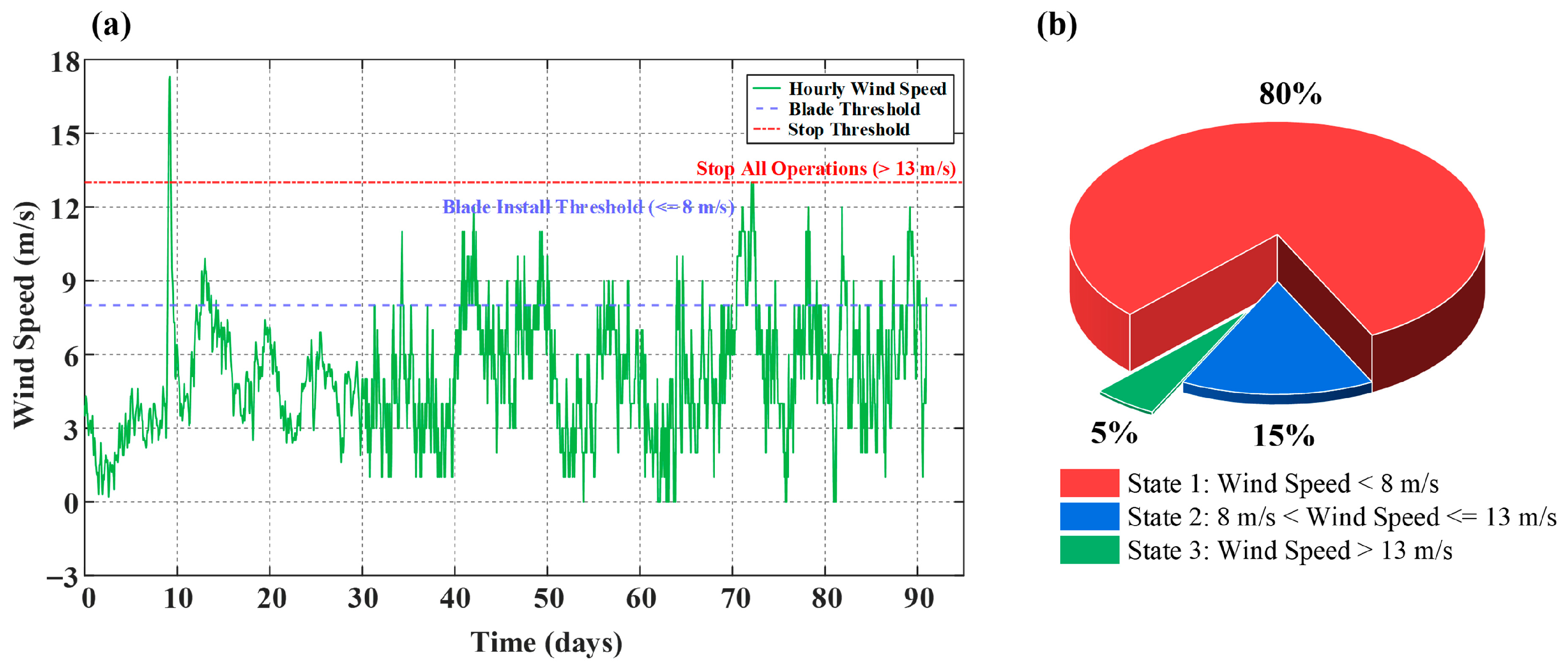
The implementation of the stochastic approach is focused on the project installation site in the South China Sea, where optimal weather windows are typically from March to May and September to November. The wind speed data for this region and period has been sourced from the EPW MAP, which provides hourly records. A representative time series is depicted in Figure 10a.

In consideration of the operational constraints pertaining to the various installation components, the following weather-dependent regulations have been stipulated:

(a) Poor Weather (Wind Speed > 13 m/s): All offshore operations for both IVs and TVs are strictly prohibited.

(b) Moderate Weather (8 m/s < Wind Speed ≤ 13 m/s): Blade installation is forbidden. To optimize vessel utilization during this period, the model allows for the postponement of the current turbine’s blade installation to proceed with other non-blade installation tasks on subsequent turbines.

(c) Good Weather (Wind Speed ≤ 8 m/s): All operations are permitted.

Based on these regulations and the aforementioned database, the probability distribution of weather states was derived as follows: good weather (80%), moderate weather (15%), and poor weather (5%), as shown in Figure 10b. These values serve as input parameters for the current case study. However, the framework remains generic, allowing for the integration of alternative distributions or correlated wind-wave models suited to other geographical locations by adjusting the probability distribution. To ensure robustness and convergence, the simulation was executed over 1000 iterations, taking the worst-case weather delay (i.e., the highest cost) across iterations as the final evaluation result.

In response to the uncertainties modeled above, a contingency plan manages tasks postponed by inclement weather. These delayed installations are grouped into a remedial phase, for which the optimal recovery sequence is determined by solving a TSP. The transportation strategy adopts the EDF-SA method with component-wise transport, which has been identified as the most cost-effective under deterministic conditions.

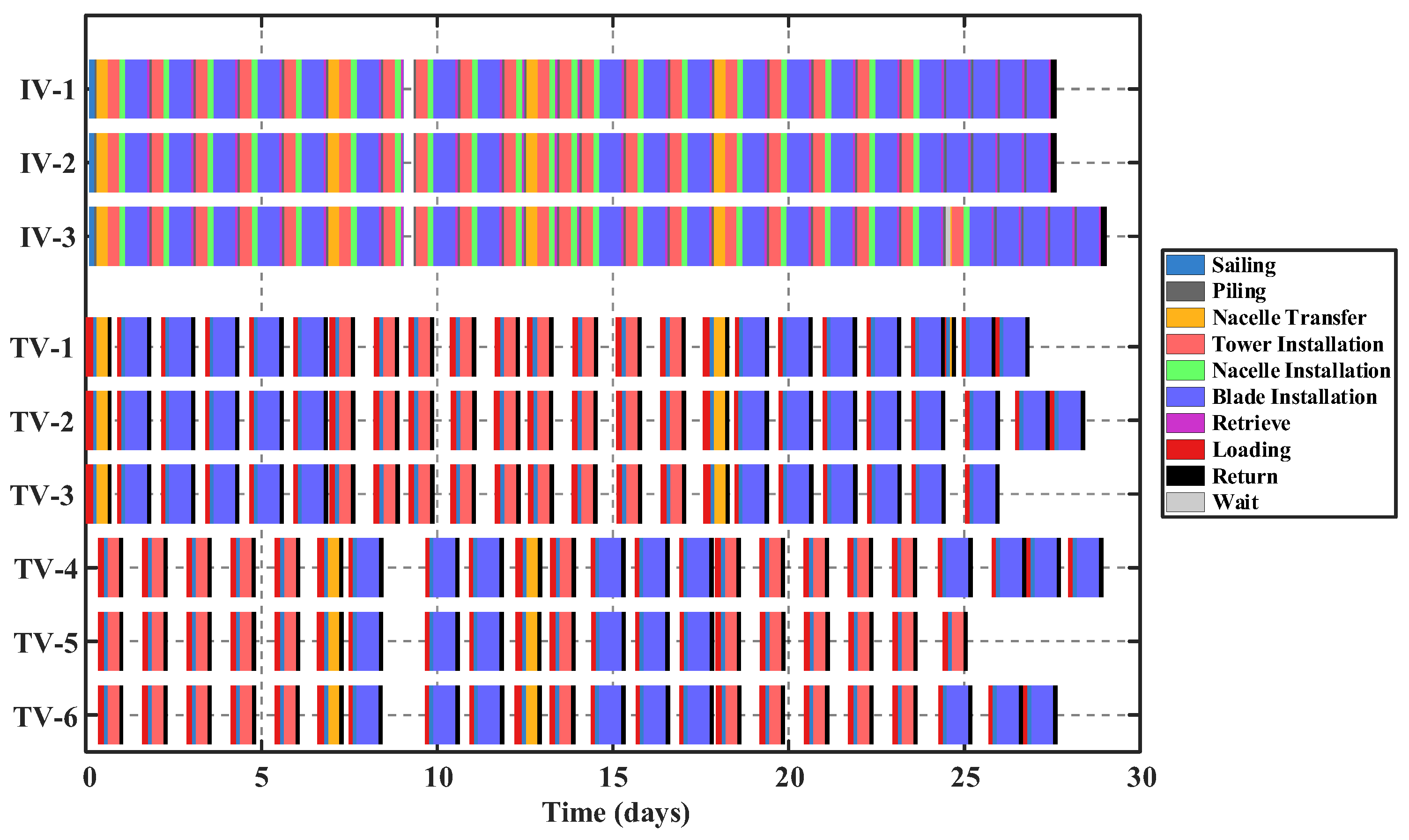
The direct operational impacts of weather variability on operations are clearly visualized in the Gantt chart for Wind Farm 2, with three IVs deployed, as presented in Figure 11. The chart reveals two distinct weather-driven disruptions. Firstly, a complete operational shutdown occurs around Day 10, a direct consequence of simulated wind speeds exceeding the 13 m/s universal threshold. Secondly, extended periods of moderate wind (8–13 m/s) around Days 10 and 13 necessitate the deferral of blade installation tasks. These tasks are then rescheduled and consolidated toward the end of the project timeline.

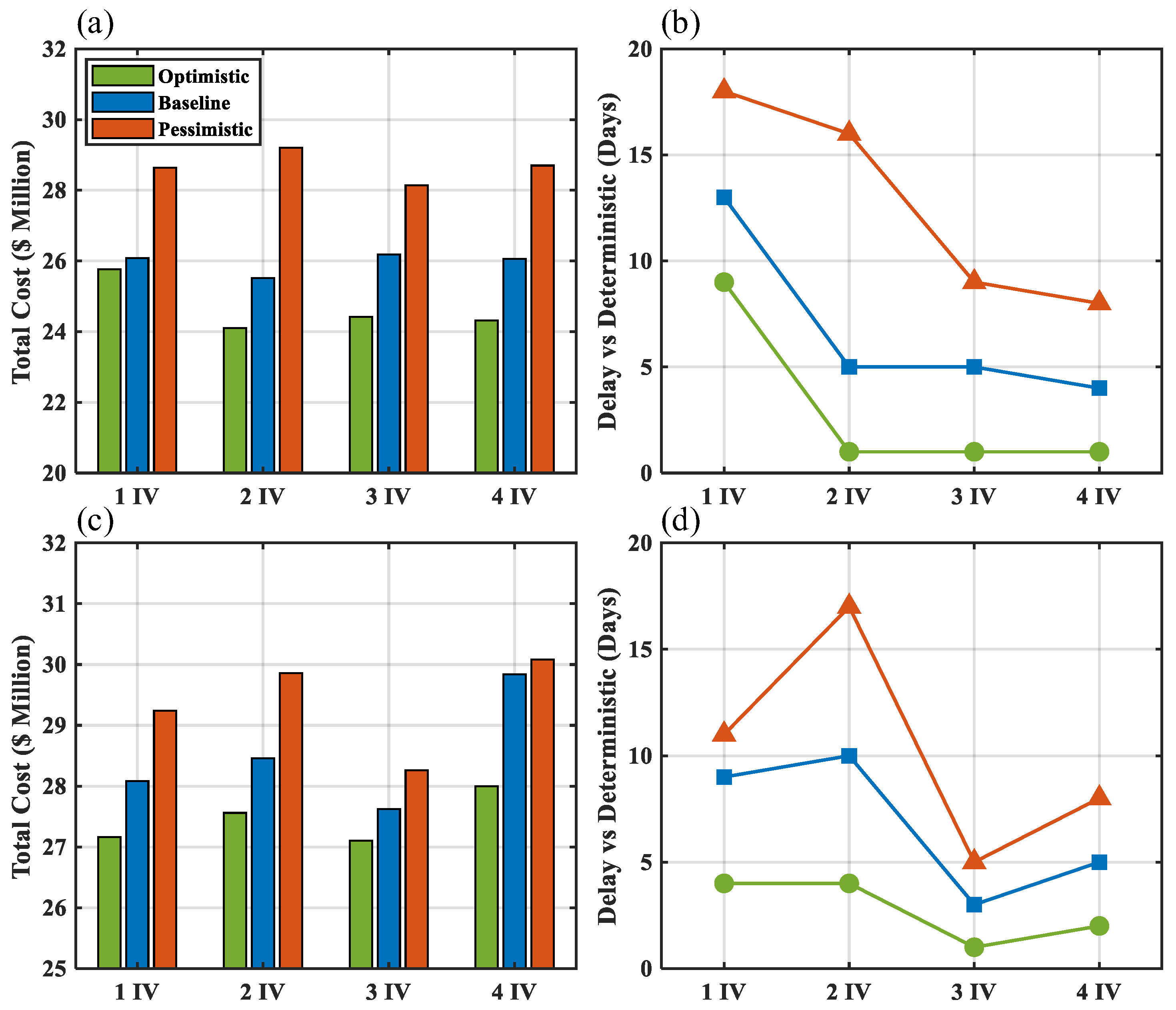
To further verify the reliability of the model, we adjusted the probability distribution to conduct a sensitivity analysis. With the initial distribution serving as the baseline, two alternative scenarios were examined. The Optimistic scenario assumes a higher frequency of favorable windows, with 85% good, 10% moderate, and 5% poor weather. Conversely, the Pessimistic scenario simulates a harsher season (75% good, 20% moderate, and 5% poor weather), thereby increasing the frequency of disruptions specific to blade installation.

The results of this analysis are presented in Figure 12, where Figure 12a,c illustrate the impact of weather severity on Total Cost, while Figure 12b,d detail the Schedule Delays relative to the deterministic duration.

As shown in Figure 12a,c, project costs consistently increase as weather conditions deteriorate from Optimistic to Pessimistic scenarios. However, a critical divergence in optimal fleet configuration is observed between the two wind farms. For Wind Farm 1, a configuration of 2 IVs and 4 TVs is optimal under baseline conditions ($25,520,000), but a strategic shift is observed under the Pessimistic scenario. The cost of the 2-IV fleet rises sharply to $29,200,000, making the larger 3-IV fleet ($28,140,000) the more cost-effective option. This suggests that increasing fleet size can serve as a hedge against severe weather delays. In contrast, the optimal strategy for Wind Farm 2 exhibits remarkable stability. Despite cost escalations under adverse weather, the configuration of 3 IVs remains the most cost-effective option across all scenarios. This indicates that for larger-scale projects, the operational redundancy provided by a larger fleet consistently outweighs the additional daily rental costs, offering robust resilience against meteorological uncertainty.

To quantify the value of the stochastic solution, we compared the baseline results with a deterministic model that assumes idealized conditions as shown in Figure 12b,d. Across all scenarios, increasing the fleet size proves effective in mitigating weather-induced slippage, yet the marginal benefits differ by project scale. Specifically, for Wind Farm 1, a substantial reduction in delay is achieved when expanding the fleet from 1 IV to 2 IVs. The steep downward trend indicates that a single vessel is highly vulnerable to restricted weather windows, often leading to prolonged downtimes. In contrast, the 2-IV configuration offers a robust buffer, significantly stabilizing the project duration and minimizing the variance between the Optimistic and Pessimistic scenarios. For the larger-scale Wind Farm 2, the data highlights the necessity of operational redundancy. Smaller fleets comprising 1 or 2 IVs suffer from significant and unpredictable delays, particularly under adverse conditions. However, the deployment of 3 IVs demonstrates a marked convergence in schedule performance. This stability implies that the improved work efficiency of the 3-IV fleet effectively neutralizes the impact of the Pessimistic weather patterns, ensuring schedule predictability despite meteorological uncertainties.

To quantify the specific economic benefits of the proposed optimization algorithm, we compared the costs of the initial scheduling schemes against the optimized schedules. Both scenarios account for stochastic weather conditions. The results of this comparison are detailed in

Table 5. Comparison of project costs between initial and optimized schedules under stochastic weather conditions.

Wind Farm	IV/TV	Initial Schedule	Schedule Optimization	Cost Reduction Rate
Wind Farm 1	2/4	$30,180,000	$25,520,000	15.44%
Wind Farm 2	3/6	$31,820,000	$27,620,000	13.20%

. As the data indicates, the application of the optimization algorithm leads to significant cost savings. Specifically, the total project costs for Wind Farm 1 and Wind Farm 2 decreased by 15.44% and 13.20%, respectively.

7. Discussion and Conclusions

This paper proposes a constraint-driven hierarchical optimization framework for the installation of OWFs. Recognizing the complexity of the MILP formulation, the solution process is decomposed into two interrelated sub-problems: path planning and scheduling optimization. For the path planning component, formulated as an MTSP, a hybrid algorithm is employed that integrates a balanced sweep clustering algorithm with nearest neighbor and 2-opt local search algorithms. This approach ensures that the vessel routes are geometrically efficient and operationally balanced. Subsequently, for scheduling optimization, an EDF-SA algorithm is utilized to minimize total installation costs, incorporating practical constraints such as the number of vessels and the waiting time of the installation vessel.

The efficacy of the proposed framework is substantiated by case studies of the Jinwan and Poseidon wind farms. Under deterministic conditions, the model evaluated distinct transport strategies and identified the component-wise transport strategy using EDF-SA as superior. This approach achieved significant cost reductions of 17.18% and 14.81% for Wind Farm 1 and Wind Farm 2, respectively, compared to initial plans. Furthermore, comparative analysis against GA and pure SA validates that the EDF-SA hybrid achieves an optimal trade-off between solution quality and computational efficiency.

To enhance practical applicability, this study incorporates a stochastic model utilizing historical wind data to address environmental uncertainty. Sensitivity analysis reveals that increasing fleet size acts as a necessary hedge against delays for smaller projects (Wind Farm 1), whereas for larger projects (Wind Farm 2), it provides operational robustness that outweighs additional costs regardless of weather severity. Even under these stochastic conditions, the optimization algorithm demonstrated robust performance. The optimized schedules considering weather uncertainty resulted in total cost reductions of 15.44% and 13.20% for Wind Farm 1 and Wind Farm 2, respectively. These findings confirm that the proposed method effectively balances economic objectives with the need for resilience against environmental disruptions.

The methodology established in this study is equally scalable to other scheduling problems, such as maintenance scheduling for OWFs. It is recommended that future research incorporate supplementary cost factors, such as inventory management and human resource scheduling, with a view to enhancing the model’s alignment with practical engineering requirements.

References

1. Khan, M.; Al-Ammar, E.A.; Naeem, M.R.; Ko, W.; Choi, H.-J.; Kang, H.-K. Forecasting Renewable Energy for Environmental Resilience through Computational Intelligence. PLoS ONE 2021, 16, e0256381. [Google Scholar] [CrossRef] [Scilit]
2. Zhou, B.; Zhang, Z.; Li, G.; Yang, D.; Santos, M. Review of Key Technologies for Offshore Floating Wind Power Generation. Energies 2023, 16, 710. [Google Scholar] [CrossRef] [Scilit]
3. Wu, X.; Hu, Y.; Li, Y.; Yang, J.; Duan, L.; Wang, T.; Adcock, T.; Jiang, Z.; Gao, Z.; Lin, Z.; et al. Foundations of Offshore Wind Turbines: A Review. Renew. Sustain. Energy Rev. 2019, 104, 379–393. [Google Scholar] [CrossRef] [Scilit]
4. Díaz, H.; Guedes Soares, C. Review of the Current Status, Technology and Future Trends of Offshore Wind Farms. Ocean Eng. 2020, 209, 107381. [Google Scholar] [CrossRef] [Scilit]
5. Osman, A.I.; Chen, L.; Yang, M.; Msigwa, G.; Farghali, M.; Fawzy, S.; Rooney, D.W.; Yap, P.-S. Cost, Environmental Impact, and Resilience of Renewable Energy under a Changing Climate: A Review. Environ. Chem. Lett. 2023, 21, 741–764. [Google Scholar] [CrossRef] [Scilit]
6. Guo, Y.; Wang, H.; Lian, J. Review of Integrated Installation Technologies for Offshore Wind Turbines: Current Progress and Future Development Trends. Energy Convers. Manag. 2022, 255, 115319. [Google Scholar] [CrossRef] [Scilit]
7. Jing, Z.; Feng, H. Selection and Application of China Environmental Sustainability Policy Instrumental: A Quantitative Analysis Based on “Dual Carbon” Policy Text. Front. Environ. Sci. 2024, 12, 1418253. [Google Scholar] [CrossRef] [Scilit]
8. Zhang, X.; Liang, D.; Zhang, S. The Impact of Digital–Financial Dual Pilot Policy on Carbon Emission Efficiency: Evidence from Chinese Cities. Land 2025, 14, 686. [Google Scholar] [CrossRef] [Scilit]
9. Anuta, H.; Ralon, P.; Taylor, M. Renewable Power Generation Costs in 2018; International Renewable Energy Agency (IRENA): Masdar City, United Arab Emirates, 2019. [Google Scholar]
10. Jiang, Z. Installation of Offshore Wind Turbines: A Technical Review. Renew. Sustain. Energy Rev. 2021, 139, 110576. [Google Scholar] [CrossRef] [Scilit]
11. Tautz-Weinert, J.; Watson, S.J. Using SCADA Data for Wind Turbine Condition Monitoring—A Review. IET Renew. Power Gener. 2017, 11, 382–394. [Google Scholar] [CrossRef] [Scilit]
12. Myhr, A.; Bjerkseter, C.; Ågotnes, A.; Nygaard, T.A. Levelised Cost of Energy for Offshore Floating Wind Turbines in a Life Cycle Perspective. Renew. Energy 2014, 66, 714–728. [Google Scholar] [CrossRef] [Scilit]
13. Taylor, M.; Ralon, P.; Ilas, A. The Power to Change: Solar and Wind Cost Reduction Potential to 2025; International Renewable Energy Agency (IRENA): Masdar City, United Arab Emirates, 2016. [Google Scholar]
14. Frijlink, T.; Fazi, S.; Tavasszy, L.; Duinkerken, M.; Lammers, L. A Decision Support Framework for the Evaluation of Installation Strategies of Superstructures for Offshore Wind Farms. Ocean Eng. 2025, 329, 121144. [Google Scholar] [CrossRef] [Scilit]
15. Song, S.; Li, Q.; Felder, F.A.; Wang, H.; Coit, D.W. Integrated Optimization of Offshore Wind Farm Layout Design and Turbine Opportunistic Condition-Based Maintenance. Comput. Ind. Eng. 2018, 120, 288–297. [Google Scholar] [CrossRef] [Scilit]
16. Le Pivert, F.; Roberts, A.; López-Santander, A.; Craven, M.J.; Kazemi, S. Data Driven Multi-Objective Optimization of the Scheduling for Towing a Floating Offshore Wind Turbine between Assembly Port and Installation Location throughout a Year. Appl. Ocean Res. 2025, 157, 104492. [Google Scholar] [CrossRef] [Scilit]
17. Barlow, E.; Tezcaner Öztürk, D.; Revie, M.; Akartunalı, K.; Day, A.H.; Boulougouris, E. A Mixed-Method Optimisation and Simulation Framework for Supporting Logistical Decisions during Offshore Wind Farm Installations. Eur. J. Oper. Res. 2018, 264, 894–906. [Google Scholar] [CrossRef] [Scilit]
18. Irawan, C.A.; Jones, D.; Ouelhadj, D. Bi-Objective Optimisation Model for Installation Scheduling in Offshore Wind Farms. Comput. Oper. Res. 2017, 78, 393–407. [Google Scholar] [CrossRef] [Scilit]
19. Ursavas, E. A Benders Decomposition Approach for Solving the Offshore Wind Farm Installation Planning at the North Sea. Eur. J. Oper. Res. 2017, 258, 703–714. [Google Scholar] [CrossRef] [Scilit]
20. Amorosi, L.; Fischetti, M.; Paradiso, R.; Roberti, R. Optimization Models for the Installation Planning of Offshore Wind Farms. Eur. J. Oper. Res. 2024, 315, 1182–1196. [Google Scholar] [CrossRef] [Scilit]
21. Sarker, B.R.; Faiz, T.I. Minimizing Transportation and Installation Costs for Turbines in Offshore Wind Farms. Renew. Energy 2017, 101, 667–679. [Google Scholar] [CrossRef] [Scilit]
22. Irawan, C.A.; Song, X.; Jones, D.; Akbari, N. Layout Optimisation for an Installation Port of an Offshore Wind Farm. Eur. J. Oper. Res. 2017, 259, 67–83. [Google Scholar] [CrossRef] [Scilit]
23. Kweon, S.J.; Hwang, S.W.; Lee, S.; Jo, M.J. Demurrage Pattern Analysis Using Logical Analysis of Data: A Case Study of the Ulsan Port Authority. Expert Syst. Appl. 2022, 206, 117745. [Google Scholar] [CrossRef] [Scilit]
24. Venturini, G.; Iris, Ç.; Kontovas, C.A.; Larsen, A. The Multi-Port Berth Allocation Problem with Speed Optimization and Emission Considerations. Transp. Res. Part D Transp. Environ. 2017, 54, 142–159. [Google Scholar] [CrossRef] [Scilit]
25. Kang, J.; Guedes Soares, C. An Opportunistic Maintenance Policy for Offshore Wind Farms. Ocean Eng. 2020, 216, 108075. [Google Scholar] [CrossRef] [Scilit]
26. Stock-Williams, C.; Swamy, S.K. Automated Daily Maintenance Planning for Offshore Wind Farms. Renew. Energy 2019, 133, 1393–1403. [Google Scholar] [CrossRef] [Scilit]
27. De Matos Sá, M.; Correia Da Fonseca, F.X.; Amaral, L.; Castro, R. Optimising O&M Scheduling in Offshore Wind Farms Considering Weather Forecast Uncertainty and Wake Losses. Ocean Eng. 2024, 301, 117518. [Google Scholar] [CrossRef] [Scilit]
28. Lu, Y.; Sun, L.; Xue, Y. Research on a Comprehensive Maintenance Optimization Strategy for an Offshore Wind Farm. Energies 2021, 14, 965. [Google Scholar] [CrossRef] [Scilit]
29. Bertsimas, D.; Brown, D.B.; Caramanis, C. Theory and Applications of Robust Optimization. SIAM Rev. 2011, 53, 464–501. [Google Scholar] [CrossRef] [Scilit]
30. Chao, H.; Hu, B.; Xie, K.; Tai, H.-M.; Yan, J.; Li, Y. A Sequential MCMC Model for Reliability Evaluation of Offshore Wind Farms Considering Severe Weather Conditions. IEEE Access 2019, 7, 132552–132562. [Google Scholar] [CrossRef] [Scilit]
31. Peng, S.; Rippel, D.; Becker, M.; Szczerbicka, H. Scheduling of Offshore Wind Farm Installation Using Simulated Annealing. IFAC-PapersOnLine 2021, 54, 325–330. [Google Scholar] [CrossRef] [Scilit]
32. Dighe, V.V.; Liu, Y. Advancing Weather Predictions for Offshore Wind Farm Maintenance through Deep Learning. J. Phys. Conf. Ser. 2024, 2767, 092091. [Google Scholar] [CrossRef] [Scilit]
33. Hadjoudj, Y.; Pandit, R.K. Improving O&M Decision Tools for Offshore Wind Farm Vessel Routing by Incorporating Weather Uncertainty. IET Renew. Power Gener. 2023, 17, 1488–1499. [Google Scholar] [CrossRef] [Scilit]
34. Kolios, A.; Richmond, M.; Koukoura, S.; Yeter, B. Effect of Weather Forecast Uncertainty on Offshore Wind Farm Availability Assessment. Ocean Eng. 2023, 285, 115265. [Google Scholar] [CrossRef] [Scilit]
35. Hou, P.; Enevoldsen, P.; Hu, W.; Chen, C.; Chen, Z. Offshore Wind Farm Repowering Optimization. Appl. Energy 2017, 208, 834–844. [Google Scholar] [CrossRef] [Scilit]
36. Gonzalez-Rodriguez, A.G. Review of Offshore Wind Farm Cost Components. Energy Sustain. Dev. 2017, 37, 10–19. [Google Scholar] [CrossRef] [Scilit]
37. Fan, D.; Ren, Y.; Feng, Q.; Zhu, B.; Liu, Y.; Wang, Z. A Hybrid Heuristic Optimization of Maintenance Routing and Scheduling for Offshore Wind Farms. J. Loss Prev. Process Ind. 2019, 62, 103949. [Google Scholar] [CrossRef] [Scilit]
38. Fischetti, M.; Pisinger, D. Mathematical Optimization and Algorithms for Offshore Wind Farm Design: An Overview. Bus. Inf. Syst. Eng. 2019, 61, 469–485. [Google Scholar] [CrossRef] [Scilit]
39. Tao, S.; Xu, Q.; Feijoo, A.; Zheng, G. Joint Optimization of Wind Turbine Micrositing and Cabling in an Offshore Wind Farm. IEEE Trans. Smart Grid 2021, 12, 834–844. [Google Scholar] [CrossRef] [Scilit]
40. Breton, S.-P.; Moe, G. Status, Plans and Technologies for Offshore Wind Turbines in Europe and North America. Renew. Energy 2009, 34, 646–654. [Google Scholar] [CrossRef] [Scilit]
41. Ren, Z.; Verma, A.S.; Li, Y.; Teuwen, J.J.E.; Jiang, Z. Offshore Wind Turbine Operations and Maintenance: A State-of-the-Art Review. Renew. Sustain. Energy Rev. 2021, 144, 110886. [Google Scholar] [CrossRef] [Scilit]
42. Li, H.; Guedes Soares, C.; Huang, H.-Z. Reliability Analysis of a Floating Offshore Wind Turbine Using Bayesian Networks. Ocean Eng. 2020, 217, 107827. [Google Scholar] [CrossRef] [Scilit]
43. Irawan, C.A.; Wall, G.; Jones, D. An Optimisation Model for Scheduling the Decommissioning of an Offshore Wind Farm. OR Spectr. 2019, 41, 513–548. [Google Scholar] [CrossRef] [Scilit]
44. Peng, Z.; Sun, S.; Tong, L.; Fan, Q.; Wang, L.; Liu, D. Optimization of Offshore Wind Farm Inspection Paths Based on K-Means-GA. PLoS ONE 2024, 19, e0303533. [Google Scholar] [CrossRef] [Scilit]
45. Baydogmus, G. Solution for TSP/mTSP with an Improved Parallel Clustering and Elitist ACO. Comput. Sci. Inf. Syst. 2023, 20, 195–214. [Google Scholar] [CrossRef] [Scilit]
46. Ergüven, E.; Polat, F. Relative Distances Approach for Multi-Traveling Salesmen Problem. Knowl.-Based Syst. 2024, 300, 112160. [Google Scholar] [CrossRef] [Scilit]
47. Yoon, S.; Woo, S.; Kim, J.; Hwang, S.W.; Kweon, S.J. The Location Routing Problem for Cooling Shelters during Heat Waves. Urban Clim. 2022, 44, 101138. [Google Scholar] [CrossRef] [Scilit]
Figure 1. Main turbine installation process.
Jmse 14 00223 g001
Figure 2. Overall process for solving the deterministic scheduling problem.
Jmse 14 00223 g002
Figure 3. Wind farm locations. (a) Zhuhai Jinwan Wind Farm, (b) Swedish Poseidon Wind Farm. ((a) From https://nr.gd.gov.cn/gkmlpt/content/4/4079/post_4079712.html#3127 (accessed on 10 September 2025), and (b) from https://mst.dk/media/kapdatc0/samraadsunderlag-poseidon.pdf (accessed on 28 September 2025)).
Jmse 14 00223 g003
Figure 4. Operations research optimization results. (a) Wind Farm 1 IV routes, (b) Wind Farm 2 IV routes, (c) Wind Farm 1 vessel schedule, (d) Wind Farm 1 turbine status, (e) Wind Farm 2 vessel schedule, and (f) Wind Farm 2 turbine status.
Jmse 14 00223 g004
Figure 5. Gantt chart of schedule based on EDF. (a) Component-wise transport; (b) mixed-loading.
Jmse 14 00223 g005
Figure 6. Correlation analysis between the proxy objective value ( Z S A ) and the final total project cost ( Z ).
Jmse 14 00223 g006
Figure 7. Scheduling optimization result chart. (a) EDF-SA-component-wise-Farm 1, (b) EDF-SA-component-wise-Farm 2, (c) ED-SA-mixed-loading-Farm 1, (d) EDF-SA-mixed-loading-Farm 2. Note that the color legend is consistent with Figure 5.
Jmse 14 00223 g007
Figure 8. Comparison of time and cost for various schemes (Wind Farm 1). (a) Project duration comparison; (b) installation cost comparison.
Jmse 14 00223 g008
Figure 9. Comparison of time and cost for various schemes (Wind Farm 2). (a) Project duration comparison; (b) installation cost comparison.
Jmse 14 00223 g009
Figure 10. Weather conditions. (a) Partial time series of hourly wind speeds; (b) weather state probabilities.
Jmse 14 00223 g010
Figure 11. Gantt chart considering weather.
Jmse 14 00223 g011
Figure 12. Sensitivity analysis of project performance under varying weather scenarios (Optimistic, Baseline, and Pessimistic). (a) Total project cost for Wind Farm 1, (b) schedule delays relative to the deterministic duration for Wind Farm 1, (c) total project cost for Wind Farm 2, and (d) schedule delays for Wind Farm 2.
Jmse 14 00223 g012