Numerical Simulation of Self-Propelled Container Ship Maneuvering in Regular Waves Using a Geometry-Resolved Propeller Model

Abstract

Ship maneuverability in waves is governed by coupled hull–rudder–propeller interactions under wave-disturbed inflow. This study simulates the self-propelled maneuvering of the KRISO Container Ship (KCS) using the unsteady Reynolds-averaged Navier–Stokes (URANS) equations, the volume-of-fluid (VOF) method, dynamic fluid–body interaction (DFBI), an overset grid, and a geometry-resolved multiple-reference-frame (MRF) propeller. The numerical method is assessed against standard open-water propeller data and KCS zigzag and turning-circle data. Wave heading redistributed the response rather than changing all components uniformly: the following-sea case produced the largest reported resistance variation (51.99 N), the beam-sea case produced the largest heave amplitude (0.0150 m), and bow-quartering and following seas produced nearly equal pitch amplitudes (0.378° and 0.376°). Increasing the rudder angle from 17.5° to 22.5° reduced the tactical diameter from 11.25 m to 7.14 m (36.5%) but increased the estimated transient roll-growth slope from 0.013°/s to 0.035°/s (about 2.7 times), while heave amplitude changed by only 0.0035 m. The unequal response rates reveal that tighter turning is obtained at a disproportionate roll and propulsion-unsteadiness penalty, whereas vertical translation remains comparatively weakly coupled to steering intensity.

1. Introduction

Ship maneuverability in waves is an important consideration for navigational safety and operational reliability. The e-navigation strategy of the International Maritime Organization (IMO) and the continuing development of Maritime Autonomous Surface Ships (MASS) also increase the need for reliable performance assessment under realistic environmental disturbances [1,2,3,4].

These developments are accelerating the transition toward cleaner, more digitalized, and increasingly autonomous maritime operations, thereby increasing the need for reliable predictions of ship maneuvering behavior under realistic wave conditions. Early work established theoretical formulations capable of describing maneuvering motions in a wave environment and laid the foundation for unified seakeeping–maneuvering analyses [5]. Skejic et al. [6] investigated ship maneuvering in waves using a two-time scale model during maneuvering and demonstrated that the incident waves may have an important influence on the maneuvering behavior. Subsequently, Yasukawa et al. [7] determined the hydrodynamic force coefficients, and maneuvering simulations were carried out for both the KVLCC2 model and a full-scale ship for validation. Zhang et al. [8] numerically studied the wave-induced motions of ships under maneuvering conditions based on the potential flow method in the time domain to determine the hydrodynamic forces. Then, based on a two-time scale model, Zhang et al. [9] divided total ship motion into low-frequency maneuvering motion and high-frequency wave-induced motion. Li et al. [10,11,12] studied the influence of shallow water and wave action on the maneuverability of multihull vessels navigating around restricted waters. Shigunov et al. [13] summarized the results of the SHOPERA international benchmark study of numerical methods for the prediction of time-average wave-induced forces and maneuvers of ships in waves. In parallel, free-running experiments have provided indispensable benchmark data for turning and zigzag maneuvers in waves [14,15,16]. More recently, unified 6-DOF models and coupled seakeeping–maneuvering simulations have further improved the physical description of ship responses during turning in waves [17,18]. At the same time, alternative approaches such as detailed self-propulsion experiments, propeller-model assessment studies, and potential–viscous hybrid frameworks have been proposed to improve either physical realism or computational efficiency [19,20,21].

Despite these advances, several limitations remain. Experimental studies provide direct evidence of maneuvering behavior in waves, but their cost is high and the range of wave, control, and propulsion conditions that can be explored systematically is still limited [22]. MMG-type, unified, and hybrid approaches are efficient and practical, but they generally rely on simplified representations of the propulsion system or on reduced-order hydrodynamic inputs, which may not fully capture the strongly unsteady interaction among the hull, rudder, and propeller under wave-disturbed inflow [23]. High-fidelity CFD has therefore become increasingly important in recent years. Kim et al. [24,25] demonstrated that free-running URANS simulations can predict KCS maneuvering behavior in different wave conditions and later extended the analysis to course-keeping and turning performance in irregular waves. However, even in CFD-based studies, the propeller is still often represented by a body-force or virtual-disk model for computational economy. Recent assessments have shown that different propeller models can noticeably affect maneuvering prediction accuracy [26]. Aram et al. [27] also compared a body-force propeller model with a transient geometry-propeller simulation; it was suggested that the level of precision of a model of a propeller may have an impact on the predicted wave-induced maneuvering response. Direct and systematic comparisons of simplified propulsion and geometry-resolved propeller models in wave-maneuvering simulations remain limited [28,29].

Against this background, numerical results are assessed using reference open-water propeller data and benchmark KCS maneuvering data. The effects of wave heading and rudder angle on turning trajectory, roll, heave, speed, and propeller thrust are then examined. The present study investigates the self-propelled maneuvering of the KCS in regular waves using a URANS VOF framework, DFBI-based ship motion, an overset grid, and a geometry-resolved MRF propeller. The adopted KCS withDTMB 4119 configuration is intended as a numerical validation and not as a representation of the propulsion arrangement of a specific commercial vessel.

2. Methodology

A viscous flow computational fluid dynamics (CFD) model is used to simulate the self-propelled maneuvering of the KCS in waves. The numerical procedure includes geometry preparation, mesh generation, solution of the governing URANS and VOF equations, DFBI-based motion, and post-processing of hydrodynamic loads, ship motions, and flow-field quantities. A time-dependent solution is required to represent wave propagation, free-surface deformation, ship motion, and steering.

2.1. Governing Equations

The flow is assumed to be incompressible, isothermal, and of constant density within each phase. Under these assumptions, the continuity equation is written as

$${\displaystyle \frac{\partial u_i}{\partial x_i}}=0$$

(1)

where $u_i$ denotes the velocity component in the $i$^th Cartesian direction and $x_i$ represents the corresponding spatial coordinate (i = 1, 2, 3). The momentum equations for the incompressible flow are given by

$${\displaystyle \frac{\partial u_i}{\partial t}}+u_j{\displaystyle \frac{\partial u_i}{\partial x_j}}=-{\displaystyle \frac{1}{\rho }}{\displaystyle \frac{\partial p}{\partial x_i}}+{\displaystyle \frac{\mu }{\rho }}{\displaystyle \frac{{\partial }^2{u}_i}{\partial x_j^2}}+F_i$$

(2)

where $u_i$ and $u_j$ are the velocity components, $t$ is time, $\rho$ is the fluid density, $p$ is the pressure, $\mu$ is the dynamic viscosity, and $F_i$ is the body-force term in the $i$^th direction. To account for turbulence effects in an engineeringly affordable manner, the instantaneous flow variables are decomposed into mean and fluctuating components according to Reynolds averaging. This leads to the Reynolds-averaged continuity and momentum equations:

$${\displaystyle \frac{\partial {\overline{u}}_i}{\partial t}}+{\overline{u}}_j{\displaystyle \frac{\partial {\overline{u}}_i}{\partial x_j}}=-{\displaystyle \frac{1}{\rho }}{\displaystyle \frac{\partial \overline{p}}{\partial x_i}}+v{\displaystyle \frac{\partial }{\partial x_j}}\left({\displaystyle \frac{\partial {\overline{u}}_i}{\partial x_j}}-\rho \overline{u_i^{\prime }{u}_j^{\prime }}\right)+F_i$$

(3)

In the above formulas, ${\overline{u}}_i$ and ${\overline{u}}_j$ are the mean velocity components in the Cartesian system (i, j = 1, 2, 3), $\nu$ is the dynamic viscosity, $-\rho \overline{u_i^{\prime }{u}_j^{\prime }}$ denotes the Reynolds stress tensor introduced by the averaging process, and ${u_i}^{\prime }$ and ${u_j}^{\prime }$ are the velocity fluctuation components. Since the Reynolds stress terms are unknown, additional closure is required through a turbulence model.

2.2. Turbulence Model

The flow around a maneuvering self-propelled ship in waves is characterized by strong streamline curvature, wake deformation, local separation, and pronounced interaction among the hull, rudder, and propeller. Direct resolution of all turbulence scales could be achieved in these circumstances, but it would be very costly to use at this moment large-scale unsteady simulations. The URANS method is therefore a practical solution to the problem of balancing computational cost with physical fidelity.

Compared with the standard k-ε formulation, the realizable model employs a variable eddy-viscosity coefficient and is suitable for flows involving rotation, separation, and high strain rates, such as the stern flow considered here. The transport equation of turbulent kinetic energy is as follows:

$$\rho {\displaystyle \frac{\partial k}{\partial t}}+\rho {\displaystyle \frac{\partial k{u}_i}{\partial x_i}}={\displaystyle \frac{\partial }{\partial x_j}}\left[{\displaystyle \frac{\partial k}{\partial x_j}}\left(\mu +{\displaystyle \frac{{\mu }_t}{{\sigma }_k}}\right)\right]+G_k-\rho \epsilon$$

(4)

where k is the turbulent kinetic energy, ε is the turbulent dissipation rate, μ_t is the turbulent eddy viscosity, G_k is the production of turbulent kinetic energy, and σ_k and σ_ε are the model constants and the transport equation for the turbulent dissipation rate, ε:

$$\rho {\displaystyle \frac{\partial \epsilon }{\partial t}}+\rho {\displaystyle \frac{\partial \epsilon u_i}{\partial x_i}}={\displaystyle \frac{\partial }{\partial x_j}}\left[{\displaystyle \frac{\partial \epsilon }{\partial x_j}}\left(\mu +{\displaystyle \frac{{\mu }_t}{{\sigma }_{\epsilon }}}\right)\right]+\rho C_{1}E\epsilon -\rho C_2{\displaystyle \frac{{\epsilon }^2}{k+\sqrt{v\epsilon }}}$$

(5)

where μ is the molecular viscosity; μ_t is the turbulent eddy viscosity; and C₁, C₂, and v_ε are the coefficients or source terms associated with the realizable k-ε formulation. This feature improves the model performance in flows with anisotropy and strong curvature effects. In this simulation, the realizable k-ε model is used. Prism layers were added to the hull, rudder, and propeller surfaces to capture the boundary-layer flow and connect the near wall mesh to the outer mesh. The realizable k-ε model used the two-layer all Y+ wall treatment. This method links the viscous sublayer with the logarithmic region and works over a wide range of Y+ values.

2.3. Propeller Numerical Model

A number of methods have been employed in CFD simulations to model marine propellers, using body-force or actuator-disk models, multiple-reference-frame (MRF) approaches, and fully transient sliding-mesh methods. Body-force models are computationally efficient but do not explicitly resolve the blade geometry or the associated blade-scale flow structures. The MRF is a practical solution because it keeps the true geometry of the propeller and does not avoid this. There is a significant expense related to the complete transient mesh deformation. The current research was carried out on the basis of the DTMB 4119. It has been summarized with the most important geometric parameters in

Table 1. Geometric parameters of the scaled DTMB 4119 research propeller used in the present numerical validation.

Parameters	Value
Diameter (D) (m)	0.0927
Number of Blades	3
Pitch Ratio (at 0.7 R)	1.804
Hub Diameter Ratio	0.2
Skew Angle (°)	0
Rake Angle (°)	0
Blade Section	NACA66-mod
Disc Area Ratio	0.6135

.

The propeller was developed from the DTMB 4119 geometry and uniformly scaled to a model-scale diameter of 0.0927 m, while the blade number, pitch ratio, hub-diameter ratio, skew and rake angles, blade-section profile, and expanded-area ratio were retained as specified in Table 1. Both the blades and the hub were explicitly resolved and meshed in the CFD model, and the same propeller geometry was used without further modification in the open-water assessment and the coupled hull–propeller–rudder simulations. A cylindrical fluid subdomain surrounding the propeller was assigned a rotating reference frame operating at the prescribed rotational speed, whereas the external fluid domain remained in the stationary reference frame, with flow information transferred across the interface between the two regions. This treatment accounts for the influence of propeller rotation on the local stern flow without requiring physical mesh rotation or repeated mesh regeneration at each time step.

It should be emphasized that the DTMB 4119 is a generic three-bladed research propeller and is not intended to represent the propeller normally fitted to a commercial container ship. It was selected because reliable open-water reference data are available, enabling the geometry-resolved MRF implementation to be assessed as a numerical validation. Consequently, the coupled KCS–DTMB 4119 configuration should be regarded as a theoretical numerical benchmark rather than a vessel-specific propulsion arrangement. Differences in blade number, loading distribution, wake adaptation, and hull–propeller–rudder interaction associated with this propeller substitution may contribute to the quantitative discrepancies between the present predictions and the standard KCS EFD data.

2.4. Hull Geometry and Principal Particulars

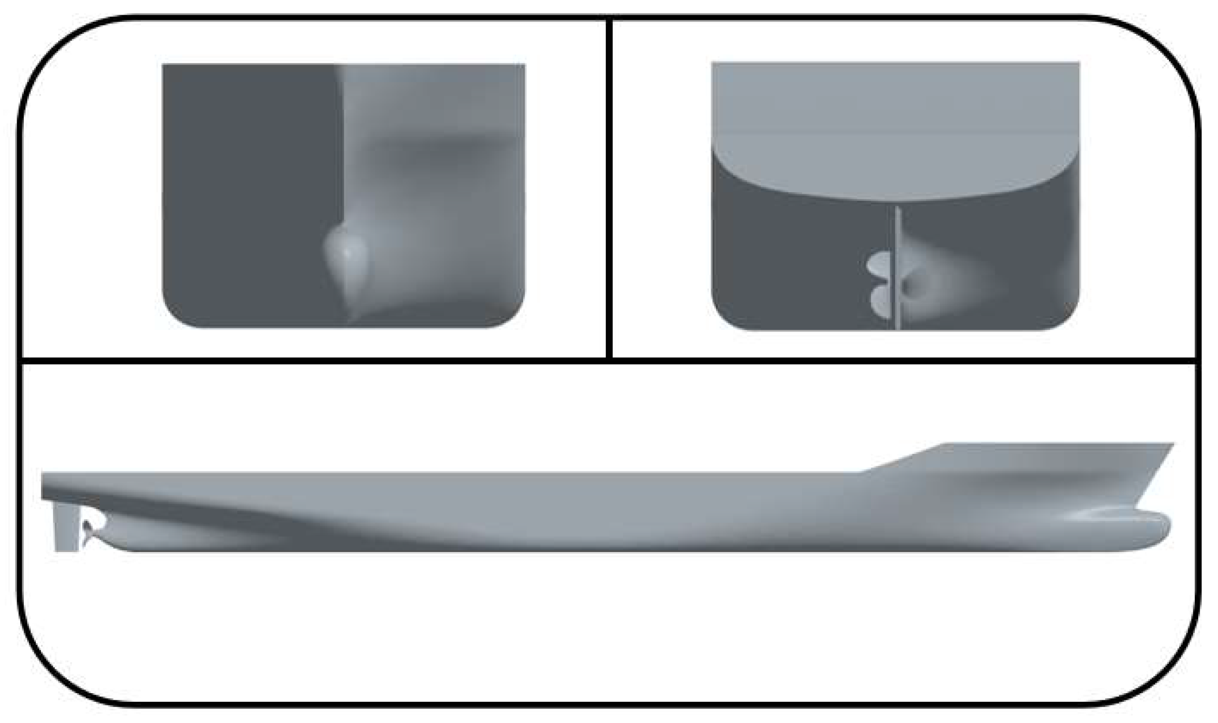
The benchmark hull considered in this study is the KCS, which has been widely used in ship hydrodynamics and maneuvering research (Figure 1). Model-scale experiments for the KCS have been reported by the University of Iowa and the Iowa Institute of Hydraulic Research (IIHR), providing an important reference for numerical validation. The principal particulars of the full-scale ship and the numerical model are listed in

Table 2. Principal particulars of full-scale and model-scale KCS.

	Full-Scale	Model-Scale
Length Between Perpendiculars (Lpp) (m)	230	2.7
Length of Waterline (LWL) (m)	232.482	2.729
Beam at Waterline (BWL) (m)	32.2	0.378
Draft (T) m	10.8	0.1268
Displacement Volume ▽ (m3)	52,061.738	0.0842
Block Coefficient CB	0.6505	0.6505
Radius of Gyration (rxx, ryy, rzz) (m)	12.88, 57.5, 57.5	0.1512, 0.675, 0.675
Distance from Center of Gravity to Baseline (KG) (m)	14.324	0.168
Transverse Metacentric Height (GM) (m)	0.623	0.0067

.

2.5. Similitude and Scale-Effect Considerations

The present computations were conducted at model scale. Based on the length between perpendiculars, the geometric scale ratio is

$${\lambda }_L={\displaystyle \frac{L_{PP,S}}{L_{PP,m}}}={\displaystyle \frac{230}{2.7}}\approx 85.19$$

Since gravitational and inertial effects dominate free-surface ship hydrodynamics, Froude similarity was adopted:

$$F_{rs}=F_{rm}, F_r={\displaystyle \frac{V}{\sqrt{gL}}}$$

Consequently, velocity and time scale with $\sqrt{{\lambda }_L}$, while wave height and wavelength scale with ${\lambda }_L$. Propeller rotational speed and rudder rate scale with ${\displaystyle \frac{1}{\sqrt{{\lambda }_L}}}$. These relationships were used to maintain consistency among the hull geometry, ship speed, wave conditions, and steering inputs.

Exact Reynolds similarity cannot be satisfied simultaneously with Froude similarity when the same fluid is used. Under Froude scaling,

$${\displaystyle \frac{R_{es}}{R_{em}}}=\sqrt[3]{{\lambda }_L.}\approx 7.9\times {10}^2$$

Therefore, the lower model-scale Reynolds number may influence the boundary layer, viscous resistance, stern wake, and the inflow to the propeller and rudder. The present results consequently represent model-scale hydrodynamic behavior and are validated against model-scale experimental data.

2.6. Grid System and Local Refinement

The numerical grid was constructed to resolve the major flow features associated with self-propelled ship maneuvering in waves, including the free-surface deformation, stern wake evolution, and local interaction among the hull, rudder, and propeller. The mesh system consists of three main parts: a body-fitted grid around the hull, locally refined regions in areas of strong flow variation, and a background grid covering the overall computational domain. An overset-grid strategy was adopted to accommodate the large-amplitude ship motions during maneuvering while maintaining mesh quality in the vicinity of the hull. The proposed approach involved applying the local mesh refinement towards the free surface, in the vicinity of areas characterized by strong hull curvature, and at the stern part up to the rudder and propeller. An additional refinement box was set around the vessel to guarantee an even transition from the near-body grid into the general background mesh. Its application enabled an accurate capture of the local hydrodynamic phenomena but did not exceed the overall computational expense limits.

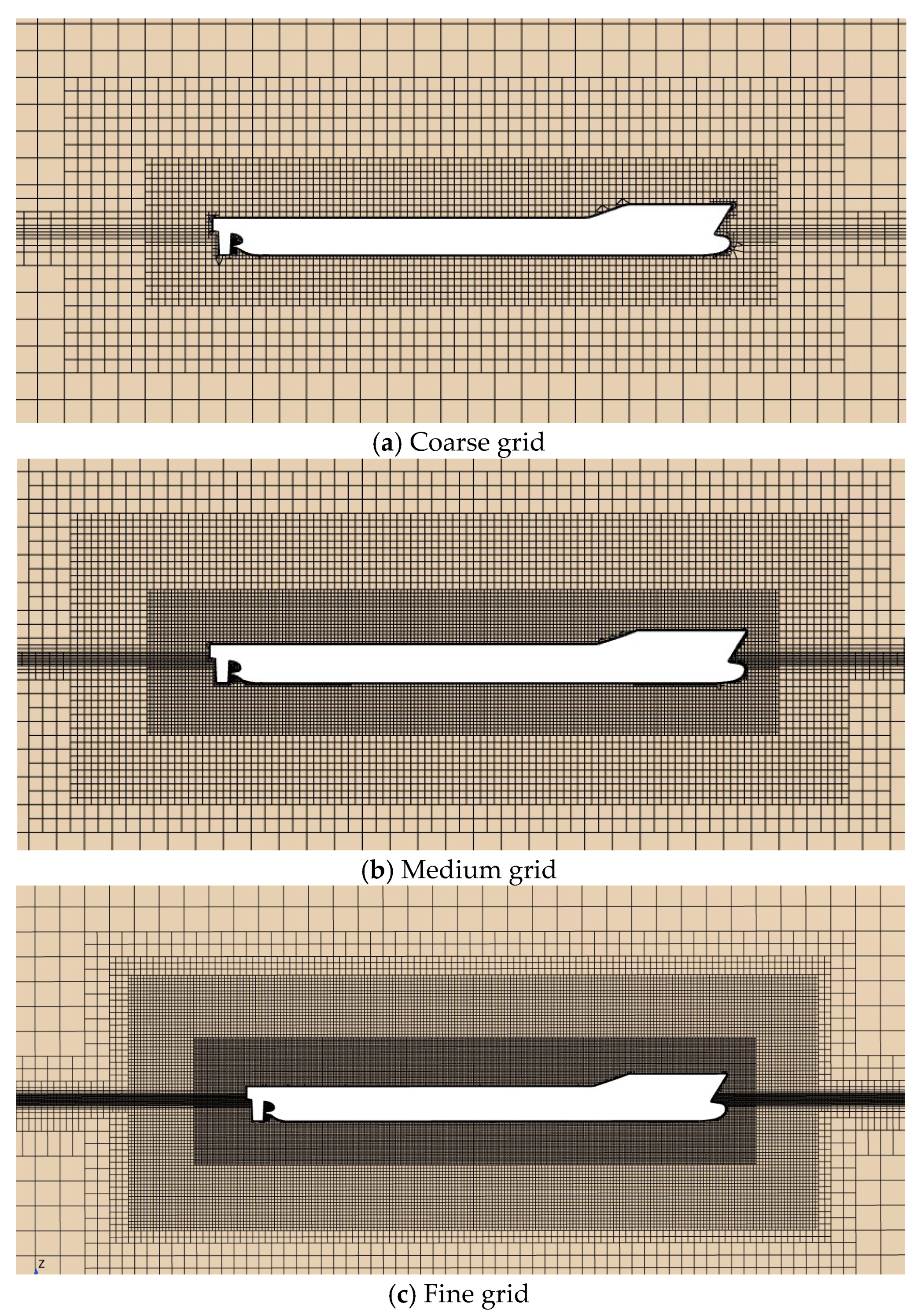
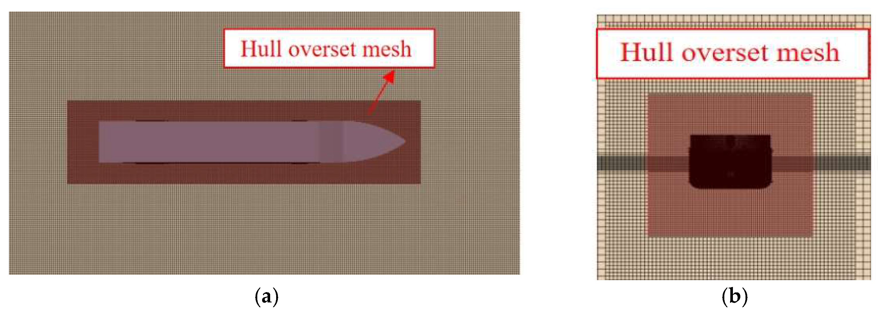
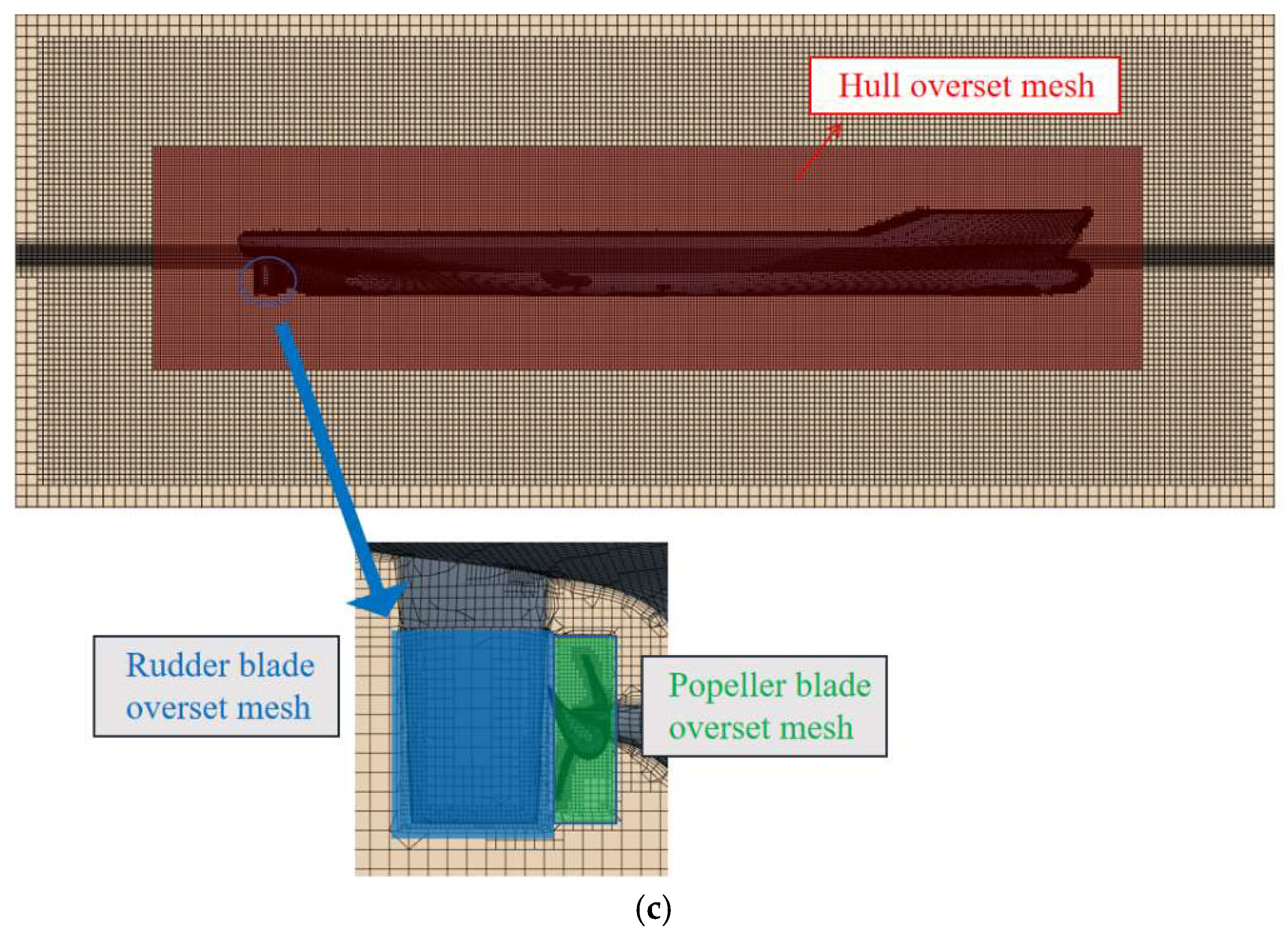
Through a rigorous grid-independence analysis, the final mesh selected for the wave maneuvering simulation consisted of approximately 4.24 million cells [12]. Figure 2 shows the implementation of the overset grid on the hull surface. An overset grid method was used to handle the large motions in the free-running maneuvering simulations. The computational domain includes a fixed background region, a hull overset region, and a rudder overset region. The hull and rudder grids can move relative to the background grid, and flow information is transferred between the overlapping regions through donor acceptor interpolation. During turning-circle and zigzag tests, the ship performs both translational and rotational motions, and the rudder rotates relative to the hull. A single deforming mesh may become highly distorted during these motions and may require repeated remeshing. This can reduce mesh quality and affect numerical stability. With the overset grid method, the body-fitted grids move with the hull and rudder, while the background grid remains fixed. This setup allows the ship to perform 6-DOF motion and the rudder angle to change without continuous deformation of the surrounding mesh.

2.7. Computational Domain and Boundary Conditions

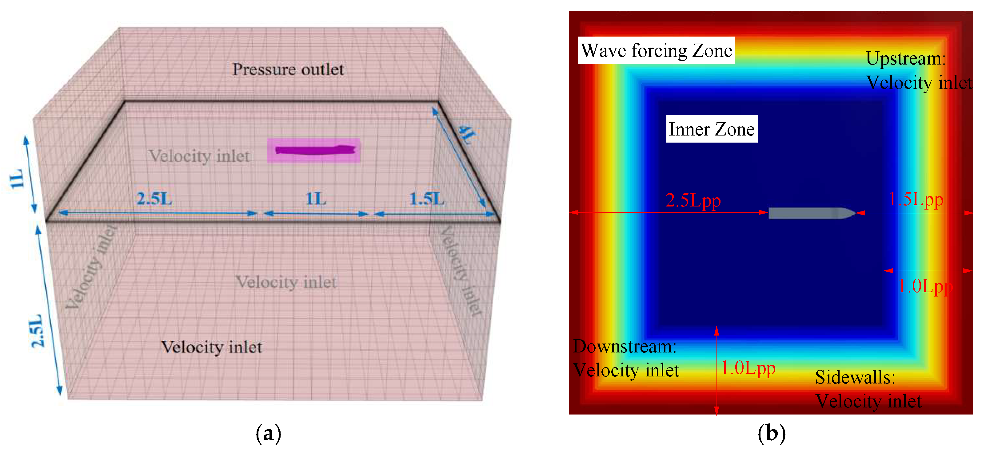
In order to analyze the current wave navigation, we will need to understand the computational domain and boundary conditions that apply to it. The simulations are based on the standard configuration usually used in free-running CFD computations in waves. The Figure 3 gives a diagrammatic representation of the overall structure of the domain layout as well as its wave absorption area. This will be facilitated by waves of incidents with various headings, the upper limits, lower limits and sides. While it is specified to be a velocity inlet boundary, at the same time the top boundary is considered as a mass flow rate outlet. This configuration enables the incident-wave kinematics to be imposed consistently for both head- and oblique-wave conditions.

To reduce the wave reflection at the outer boundaries, wave-damping zones were introduced near the inlet, outlet, and side boundaries. Within these regions, additional forcing was applied so that the local velocity and volume-fraction fields gradually relaxed toward the target wave solution. In this way, outgoing waves can be effectively absorbed and boundary reflection can be minimized. The relative regional distance used in the damping formulation is defined as the normalized distance from a given cell to the nearest boundary of the absorption zone.

The active degrees of freedom were prescribed according to the objectives of the individual simulations. In the propeller open-water calculation, no DFBI rigid-body motion was activated, and the rotational effect of the propeller was represented using the multiple-reference-frame approach. In the wave-response, zigzag, and turning-circle simulations, three degrees of freedom were activated, namely, translation along the x- and z-axes and rotation about the y-axis. The mass assigned to the DFBI ship body was 823.045 kg, and the principal moments of inertia were $I_{XX}=136.7 \mathrm{K}\mathrm{g}·{\mathrm{m}}^2, I_{yy}=117.2 \mathrm{K}\mathrm{g}·{\mathrm{m}}^2$ and $I_{zz}=2725.1 \mathrm{K}\mathrm{g}·{\mathrm{m}}^2$, with all products of inertia set to zero.

3. Validation and Verification

This section evaluates the present CFD framework in three steps. First, the open-water performance of the DTMB 4119 propeller is assessed. Second, the MRF-based maneuvering predictions are compared with the available experimental data. Third, the geometry-resolved MRF and virtual-disk propeller models are compared under the same maneuvering conditions. The experimental validation and the numerical propeller-model comparison are therefore presented and interpreted separately.

3.1. Grid-Independence Analysis

Prior to the above validation procedures, grid-independence and time-step sensitivity studies are conducted to assess the numerical discretization effects. Three systematically refined mesh resolutions are examined, while the remaining numerical settings are kept unchanged. The corresponding numerical results are compared to evaluate the influence of spatial and temporal resolutions on the predicted hydrodynamic responses. Based on these comparisons, an appropriate mesh resolution and time-step size are selected for the subsequent open-water maneuvering (Figure 4).

To quantify the spatial discretization uncertainty, a grid convergence study was carried out using the Grid Convergence Index (GCI) method based on Richardson extrapolation [30]. The fine, medium, and coarse grids are denoted by S1, S2, and S3, respectively. For a representative solution quantity, ϕ, the solution differences are defined as ε21 = ϕ2 − ϕ1 and ε32 = ϕ3 − ϕ2. The convergence ratio is calculated as RG = ε21/ε32. A value of 0 < RG < 1 indicates monotonic grid convergence. The observed order of accuracy, p, was estimated from the three systematically refined grids. The discretization uncertainty was quantified using the GCI method with the recommended safety factor. The total resistance coefficient, CT, was chosen as the representative quantity for the grid convergence assessment. The corresponding grid convergence parameters and GCI values are summarized in

Table 3. Grid-independence analysis.

Item	Symbol	Number of Cells	CT × 10−3	CT Error
Experimental value			3.711
Coarse grid	S1	1.34 M	3.124	15.8%
Medium grid	S2	2.13 M	3.456	6.9%
Fine grid	S3	4.24 M	3.629	2.2%
RG			0.521
P			2.9213
GCI12			13.1%
GCI23			6.5%
Convergence type			Monotonic convergence

.

According to the grid-independence verification analysis in Table 3, as the mesh gradually densifies from coarse to thin, the total resistance coefficient, C_T, monotonically approaches the experimental value, showing a consistent convergence trend. The errors corresponding to coarse, medium, and fine grids were 15.8%, 6.9%, and 2.2%, respectively, indicating that the fine mesh had the highest calculation accuracy and matched the test values well. The total drag coefficient C_T is defined as follows:

$$C_T={\displaystyle \frac{R_T}{0.5\rho {SU}_0^2}}$$

(6)

In the above formula, R_T is the total resistance experienced by the ship model, ρ is the density of the water, U₀ is the ship’s speed, and S is the area of the wet surface of the hull.

3.2. Time-Step-Independence Assessment

The time-step size has a direct influence on the temporal resolution, numerical stability, and computational cost of unsteady ship hydrodynamic simulations. In the present study, the time-step selection was determined by considering the characteristic time scales associated with wave propagation, propeller operation, and ship maneuvering motions. For the regular-wave conditions considered here, the model-scale wave period is approximately 1.2 s. A sufficiently small time step is therefore required to resolve the wave phase and the associated transient ship responses. In addition, the maneuvering simulations involve rapid changes in rudder-induced yaw response and unsteady propeller loading, which also require adequate temporal resolution.

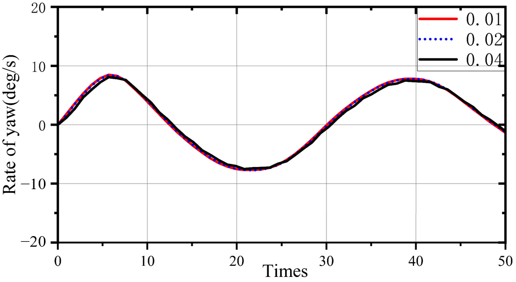
To evaluate the sensitivity of the numerical solution to the time-step size, three time steps, Δt = 0.04, 0.02, and 0.01 s, were examined. The grid configuration, physical models, wave parameters, and other numerical settings were kept unchanged. The corresponding temporal resolutions and numerical behaviors are summarized in

Table 4. Time-step sensitivity analysis.

Step, Δt [s]	Time Steps per Wave Period, T/Δt	Numerical Behavior
0.04	30	Noticeable wave-phase deviation and oscillation in the transient yaw response
0.02	60	Good agreement with the Δt = 0.01 s solution
0.01	120	Higher temporal resolution with only minor differences from Δt = 0.02 s

and Figure 5.

The calculations with Δt = 0.04 s showed noticeable phase deviations in the free-surface response. They also showed increased numerical oscillations in the transient maneuvering response. When the time step was reduced to 0.02 s, these deviations were substantially reduced. The resistance, free-surface elevation, and propeller-thrust histories obtained with Δt = 0.02 and 0.01 s showed close agreement. This indicated that the numerical solution had become nearly independent of further temporal refinement. Δt = 0.02 s provides an acceptable compromise between computational accuracy and efficiency. However, the smaller time step of Δt = 0.01 s was adopted for the subsequent zigzag and turning-circle simulations. This choice provided sufficient temporal resolution for wave-induced motions, rudder-induced transient responses, and unsteady propeller loading.

3.3. Open-Water Assessment of the Propeller Model

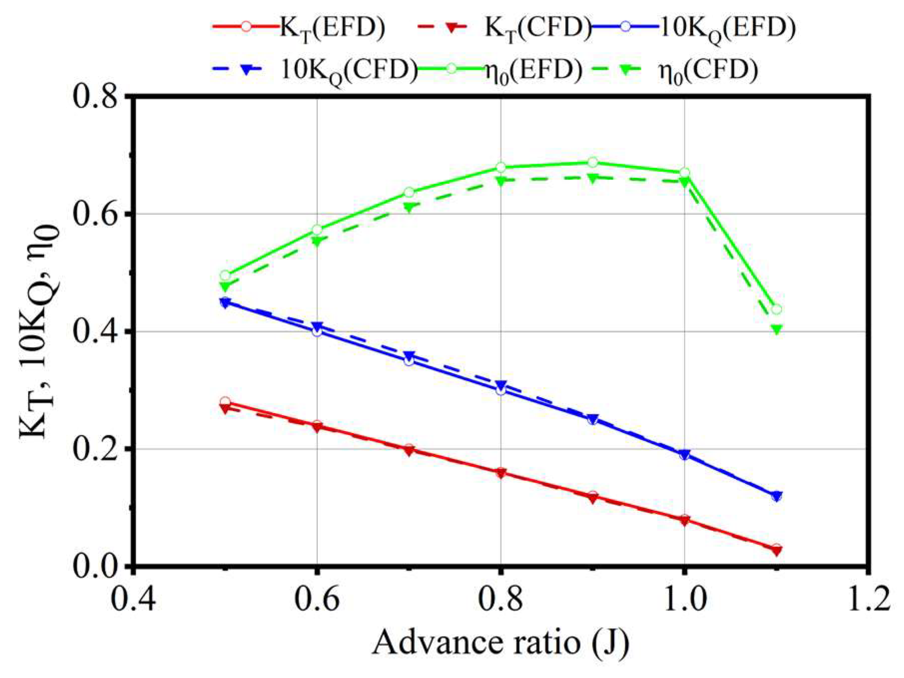
Before being integrated into the self-propelled ship simulations, the DTMB 4119 propeller model was assessed in open water by comparing the predicted hydrodynamic coefficients with reference data reported by Jessup [31]. The comparison includes the thrust coefficient, torque coefficient, and open-water efficiency, as shown in Figure 6. The mean relative errors of K_T and K_Q are approximately 6.13% and 5.12%, respectively, and the K_T error decreases to approximately 3.21% at the higher advance coefficients considered.

The agreement is acceptable for the present numerical validation. The results indicate that the geometry-resolved MRF model can reproduce the general open-water performance of DTMB 4119 with reasonable accuracy. However, this assessment verifies only the standalone open-water performance of the selected research propeller. Because the DTMB 4119 is a substitute propeller rather than a vessel-specific KCS propeller, its use may contribute to quantitative differences between the subsequent coupled simulations and the standard KCS EFD data. It should be noted that the coupled accuracy of the full hull–propeller–rudder system must still be assessed in maneuvering conditions.

3.4. Comparative Assessment of KCS Zigzag Maneuvers

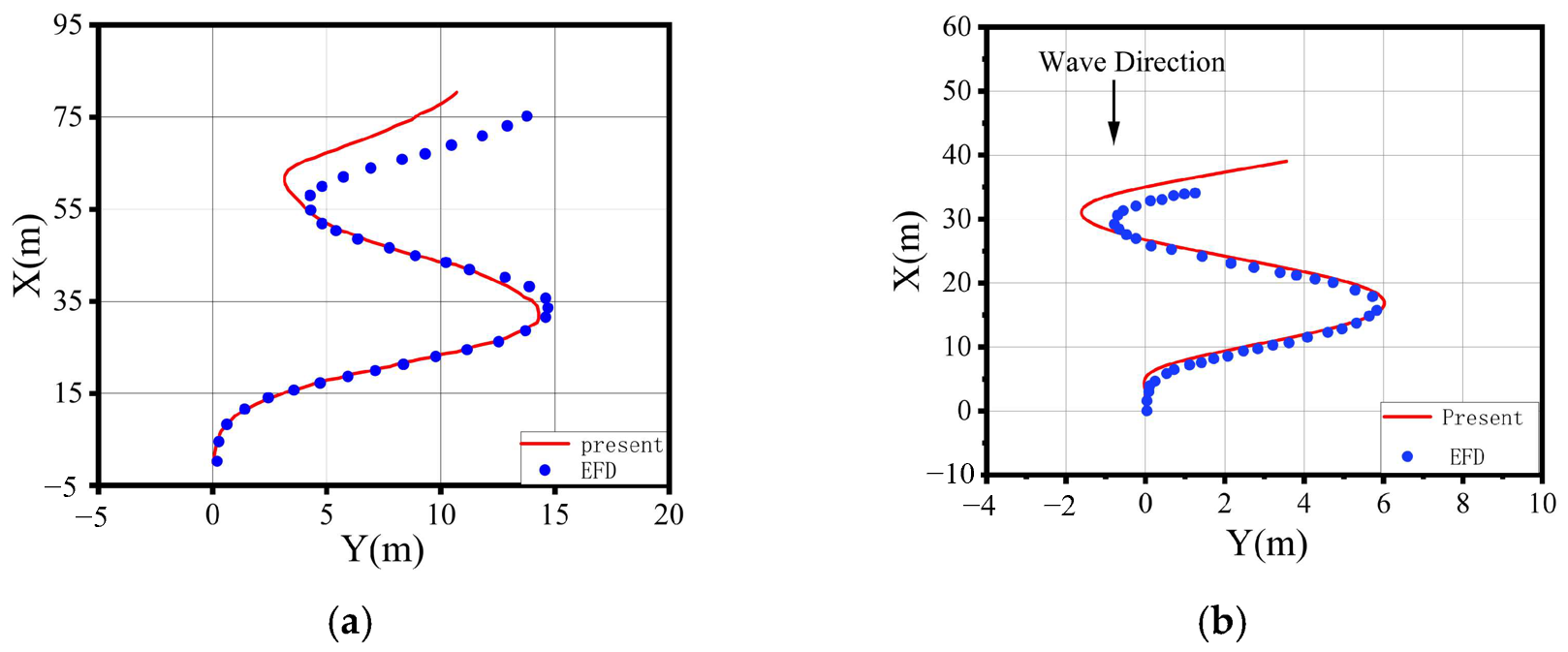
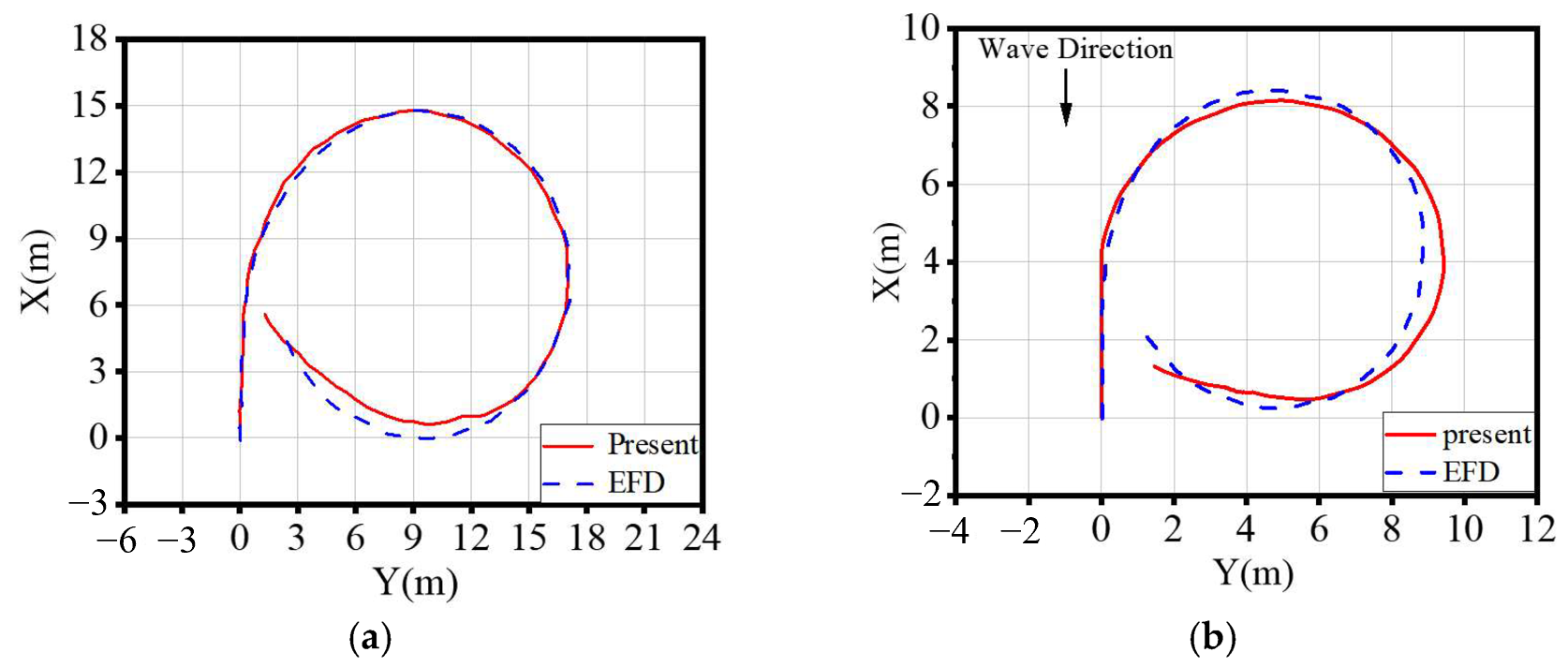
The KCS zigzag experiments were carried out under the operating conditions reported by SIMMAN [32] for calm-water and regular-wave maneuvering tests. The speed of ship was set to 14.5 kn in full scale, corresponding to a model-scale speed of 0.86 m/s (=0.16). In calm water, the self-propulsion rotational speed was 10.87 rps and the model-scale rudder rate was 14.28°/s. In waves, the propeller speed and rudder rate were kept unchanged, while the wave length-to-ship length ratio was set to 1 and the model-scale wave height was 0.048 m. Under head-wave conditions, a 20°/20° zigzag maneuver starting with a starboard rudder was simulated. The corresponding trajectory comparisons in different conditions are shown in Figure 7. The time step was 0.01 s. The background mesh was refined in the wave-height and wavelength directions to better capture the wave field.

In calm water, the present numerical results show similar overall zigzag behavior to the EFD data, although some differences can be observed in the overshoot angles and yaw-rate peaks. According to

Table 5. Comparison of zigzag maneuvering results in calm water.

Characteristic Parameter	EFD	Present	Relative Error
First Overshoot Angle (°)	23.22	22.75	−2.02%
Second Overshoot Angle (°)	21.58	20.23	−6.26%
Maximum First Yaw Rate (°/s)	7.09	6.75	−4.80%
Maximum Second Yaw Rate (°/s)	−7.61	−6.24	−18.02%

, the first and second overshoot angles predicted by the present method are 22.75° and 20.23°, compared with the EFD values of 23.22° and 21.58°, respectively. The corresponding relative differences are 2.02% and 6.26%. The relative differences in the first and second yaw-rate peaks are 4.80% and 18.02%, respectively. The larger difference in the second yaw-rate peak indicates that the transient yaw response following repeated rudder reversals is less accurately reproduced.

To provide a standard-based assessment, the calm-water 20°/20° zigzag result was evaluated against IMO Resolution MSC.137(76). According to the Resolution, the first overshoot angle in the 20°/20° zigzag test should not exceed 25°. The first overshoot angle predicted by the present model is 22.75°, indicating that the calculated result satisfies this criterion. The second overshoot angle is retained for comparison with the experimental data, although MSC.137(76) does not specify a separate limit for the second overshoot angle in the 20°/20° test. Since the IMO criteria are specified for calm-water trial conditions, the wave-case results are used for hydrodynamic-response comparison rather than formal compliance assessment. Under wave action, the difference between the present results and the EFD data becomes more pronounced during the later stage of the maneuver. As listed in

Table 6. Comparison of zigzag maneuver results in waves.

Characteristic Parameter	EFD	Present	Relative Error
First Overshoot Angle (°)	13.11	12.78	2.58%
Second Overshoot Angle (°)	18.34	16.52	−11.02%
Maximum First Yaw Rate (°/s)	6.02	5.83	−3.26%
Maximum Second Yaw Rate (°/s)	23.93	21.51	−11.25%

, the first and second overshoot angles predicted by the present method are slightly smaller than the corresponding EFD values. The present method also underpredicts the two yaw-rate peaks. The relatively larger differences during the later rudder reversal may be associated with the unsteady wave–hull–propeller–rudder interaction.

Therefore, the zigzag results indicate that the numerical propeller model produces a responsive and larger differentiated maneuvering behavior, especially under wave conditions. The present comparison therefore supports the use of the created propeller model for subsequent wave-turning simulations. The model reproduces the principal maneuvering trends with varying levels of quantitative agreement; this judgement is directionally reasonable.

3.5. Comparative Assessment of KCS Turning Maneuvers

The turning-circle simulations were performed under the same speed and wave conditions as those used in the preceding zigzag cases above. A 35° starboard turning maneuver was conducted for the KCS in regular head waves. For the wave cases, the propeller rotational speed in the self-propulsion condition was adjusted to 15.0 rps in the MRF-based resolved-propeller model so as to maintain the target approach speed. The full-scale ship speed was 14.5 kn and the initial rudder turning rate was set to 20.1°/s. The time step = 0.01 s for the numerical simulations. The purpose of this section is to compare the turning responses predicted by the geometry-resolved propeller model and the virtual propeller model under otherwise identical maneuvering conditions.

The predicted turning trajectories are shown in Figure 8, and the corresponding turning parameters are summarized in

Table 7. Comparison of turning parameters in calm water.

Characteristic Parameter	EFD	Present	Relative Error
Advance (m)	14.92	13.44	9.92%
Transfer (m)	6.05	5.71	5.62%
Tactical Diameter (m)	16.47	15.14	8.08%

and

Table 8. Comparison of turning parameters in regular head waves.

Characteristic Parameter	EFD	Present	Relative Error
Advance (m)	8.69	8.01	7.83%
Transfer (m)	3.66	3.91	6.83%
Tactical Diameter (m)	9.09	9.42	4.29%

. In calm water, the experiments give consistently larger geometric turning measures than the presented numerical model. Specifically, the advance, transfer, and tactical diameter are higher by 9.92%, 5.62%, and 8.08%, respectively. The measurement outcomes indicate that at the tranquil water level, the turning path becomes wider; however, the current findings suggest a smaller turning radius. One possible explanation is that the numerical propeller model represents in greater detail the stern–flow imbalance as well as the local hull–propeller–rudder interactions, which consequently change the effective sideways force and yawing moment while turning.

In regular head waves, CFD underpredicts advance by 7.83% and overpredicts transfer and tactical diameter by 6.83% and 4.29%, respectively. The change in the sign of the discrepancies between calm water and waves indicates sensitivity to wave-disturbed inflow and coupled steering response, but it does not demonstrate that one propulsion representation is intrinsically more accurate.

Existing studies have shown that turning characteristics in waves are highly sensitive to wave conditions and propulsion modelling. Free-running model tests on KCS in regular waves reported that the initial and steady turning characteristics vary markedly with wave height, length, heading, and approach speed. In CFD-based maneuvering studies, recent studies comparing body-force and discretized/actual propeller models confirmed that propeller-model fidelity can noticeably affect turning predictions in waves, while RANS–overset simulations with errors within roughly 10% for the main turning parameters are commonly considered acceptable [27]. Therefore, the present differences between the virtual and resolved propeller models are not abnormal in magnitude. Overall, the comparison indicates that the experiments and the CFD model led to similar qualitative turning trends, but they differ in the predicted magnitude of the turning parameters, particularly under wave conditions. These discrepancies highlight the importance of propulsion-model fidelity in wave-maneuvering simulations and support the use of the propeller model in the subsequent analyses of rudder-angle and wave-heading effects.

4. Results and Analysis

4.1. Response Characteristics Under Different Wave Headings

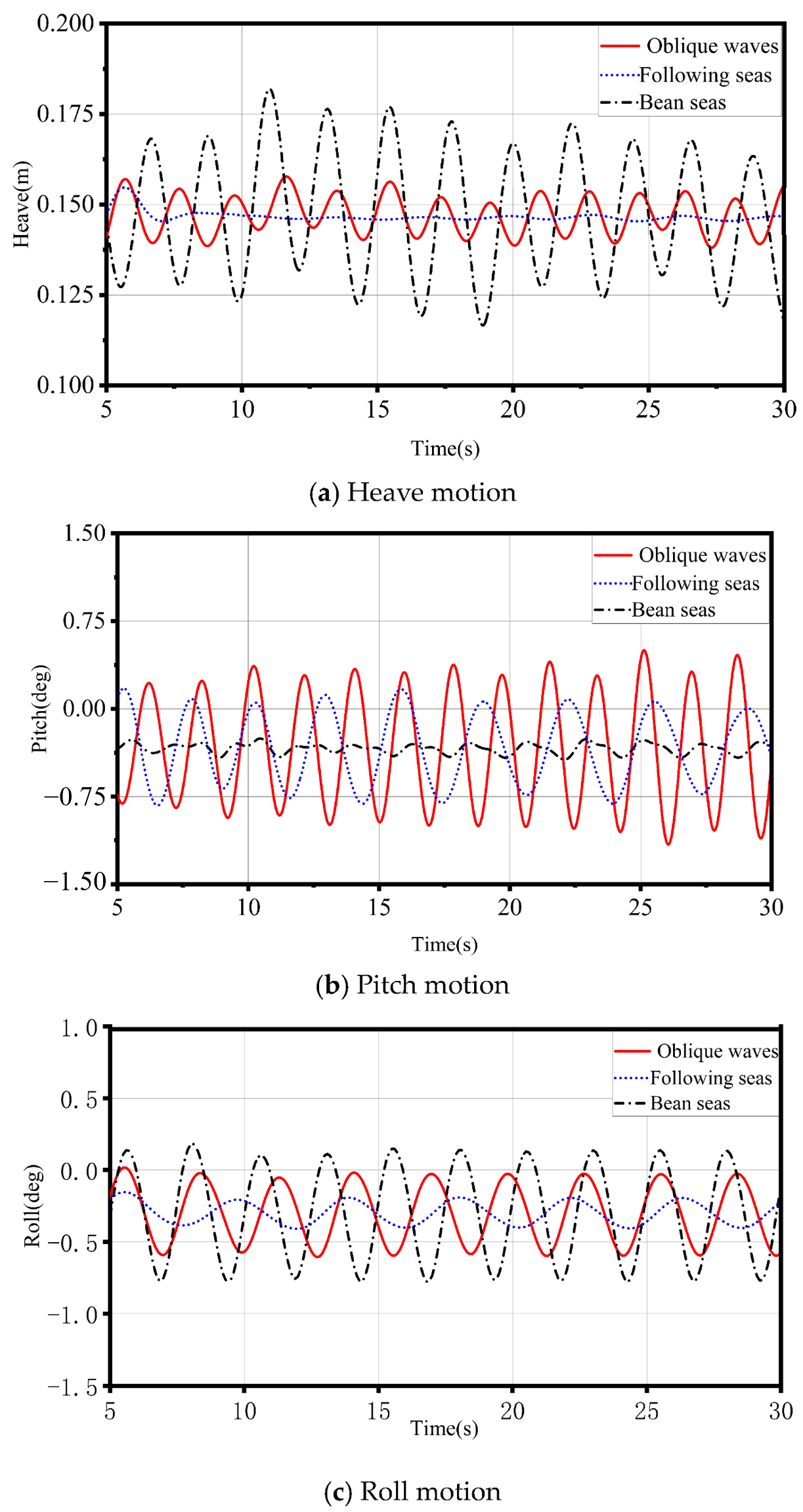
To examine the influence of wave heading on the self-propelled ship, the heave, pitch, and roll time histories obtained for three wave directions are compared in Figure 8, while the mean resistance coefficients and steady-state response amplitudes are summarized in

Table 9. Comparison of resistance and motion responses with the results of Kim et al. [16].

Wave Directions	Date Source	Mean Resistance Coefficient CR	Pitch (Deg)	Heave (m)	Roll (m)
Oblique wave (β = 225°)	Present	0.00963	0.831	0.0087	0.294
	Kim	0.0089	0.931	0.0080	-
Following wave (β = 0°)	Present	0.00618	0.446	0.00089	0.109
	Kim	0.0056	0.399	0.0010	-
Beam wave (β = 270°)	Present	0.00609	0.0870	0.00274	0.463
	Kim	0.0054	0.095	0.0250	-

. The first 5 s of each simulation was excluded to avoid startup transients. The time histories from 5 to 30 s are presented to show the evolution of the responses, whereas the amplitudes reported in Table 9 were extracted from the quasi-steady interval of 20–30 s and defined as one-half of the peak-to-peak range. Here, β denotes the azimuth of the imposed wave-propagation vector measured from the ship-fixed positive x-direction according to the STAR-CCM+ setup. The three simulated headings are β = 0° (following seas), β = 225° (oblique waves), and β = 270° (beam seas); no intermediate headings are inferred.

The comparison with Kim et al. [24] shows that the present results reproduce the same heading-dependent trends in pitch and heave. The pitch amplitude is largest in oblique waves, reaching 0.831° compared with the reference value of 0.931°, followed by 0.446° in following seas compared with 0.399°. The smallest pitch response occurs in beam seas, with amplitudes of 0.0870° and 0.095° for the present study and Kim et al. [24], respectively. The corresponding absolute relative errors are 10.7%, 11.8%, and 8.4%. Heave exhibits the opposite ranking: the beam-sea amplitude is the largest at 0.0274 m, followed by 0.0087 m in oblique waves, whereas the following-sea amplitude decreases to 0.00089 m. The corresponding reference values are 0.0250 m, 0.0080 m, and 0.0010 m, giving absolute relative errors of 9.6%, 8.8%, and 11.0%, respectively.

As shown in Figure 9, the motion responses become bounded and quasi-periodic after the initial transient, although modest cycle-to-cycle modulation remains. Oblique waves generate the strongest pitch response because the incident wave retains a substantial longitudinal component relative to the hull, producing a pronounced bow-to-stern pressure difference and pitching moment. By contrast, the beam-sea condition suppresses the longitudinal pitching moment but strengthens the vertical and transverse responses. Consequently, beam seas produce the largest heave and roll amplitudes, with the roll amplitude reaching 0.463 degrees, compared with 0.294 degrees in oblique waves and 0.109 degrees in following seas. The following-sea case therefore yields the weakest heave and roll responses, while its pitch amplitude remains appreciable.

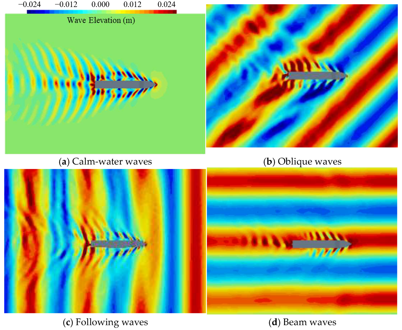
The free-surface fields in Figure 10 support this interpretation. The bow-quartering and beam cases are asymmetric about the ship centerline, whereas the following-sea field is predominantly longitudinal. Thus, heading controls not only response magnitude but also which measured response is dominant: the following case is load-dominated, the bow-quartering case retains a strong pitch response with intermediate heave, and the beam case is heave-dominated.

4.2. Influence of Rudder Angle, δ, on Turning Characteristics in Waves

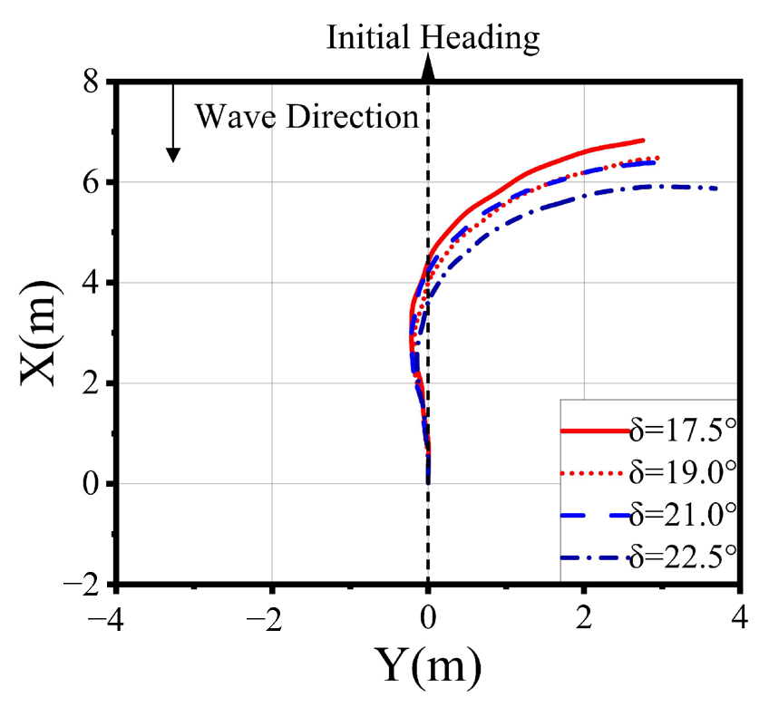
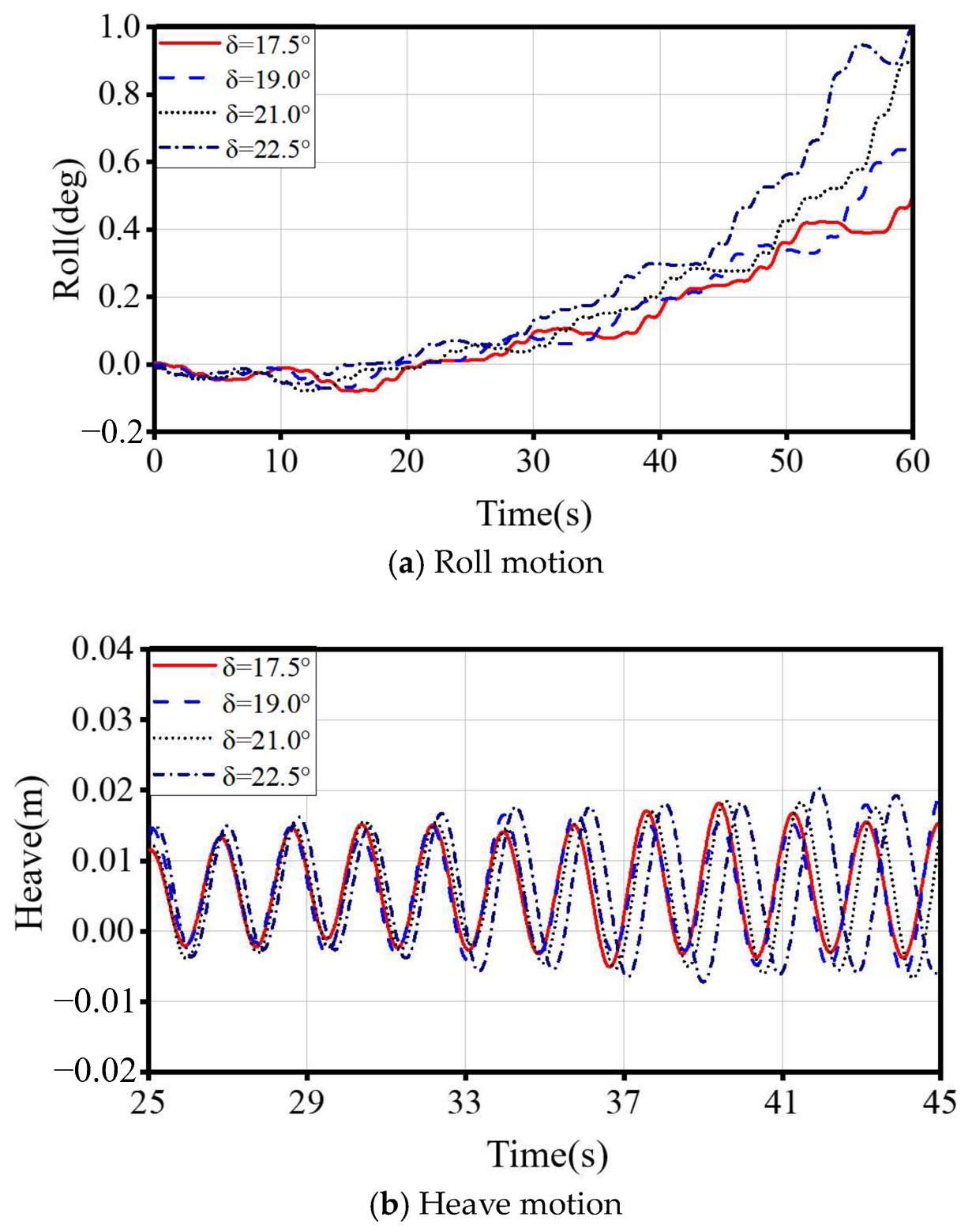
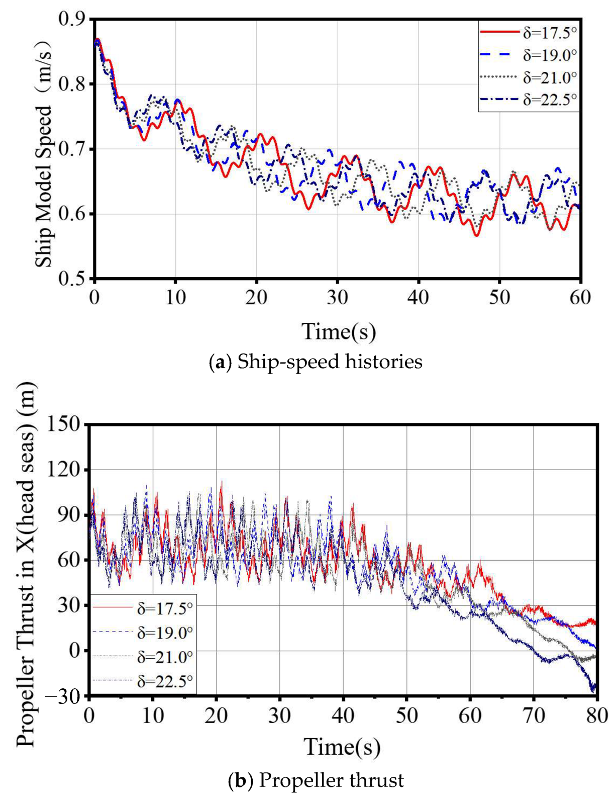
The influence of rudder angle was examined for δ = 17.5°, 19°, 21°, and 22.5°. Table 8 lists the advance, transfer, and tactical diameter results, while Figure 10, Figure 11 and Figure 12 present the trajectory, roll, heave, speed, and propeller-thrust histories. Increasing rudder angle is expected to reduce the turning dimensions; the wave-specific issue examined here is the accompanying transient motion and propulsion response.

As shown in Figure 11 and

Table 10. Effects of rudder angle on the dimensional and normalized turning parameters in regular waves.

Parameter	δ = 17.5°	δ = 19°	δ = 21°	δ = 22.5°
Advance/Lpp	3.485	3.078	2.785	2.1
Transfer/Lpp	1.819	1.522	1.422	1.081
Tactical Diameter/Lpp	4.167	3.656	1.081	2.644

, increasing δ from 17.5° to 22.5° reduces advance from 9.41 to 5.67 m, transfer from 4.91 to 2.92 m, and the tactical diameter from 11.25 to 7.14 m. Normalized by L_PP = 2.7 m, the tactical diameter decreases from 4.17L_PP to 2.64L_PP.

Figure 12a shows transient roll development rather than a converged steady response. Over the selected intervals, the roll angle increases from approximately 0.2° to 0.6° in about 30 s for δ = 17.5° and from approximately 0.2° to 0.9° in about 20 s for δ = 22.5°. The corresponding average slopes are approximately 0.013°/s and 0.035°/s. These values must not be interpreted as steady roll amplitudes or extrapolated beyond the simulated interval.

This tendency is consistent with the reduction in transfer and tactical diameter shown in Table 10. A larger rudder angle leads to a tighter turn and a smaller turning radius, which enhances the lateral acceleration and the associated heeling tendency. Under wave conditions, this effect is further amplified by the interaction between turning-induced heel and wave-excited roll. As a result, aggressive rudder commands may reduce the maneuvering margin and increase the risk of excessive heel, especially in oblique- and quartering-wave conditions. The speed and propeller-thrust histories shown in Figure 12 further indicate that larger δ values are accompanied by stronger unsteady deceleration and more pronounced thrust fluctuation. The rudder case with an angle of 22.5 degrees has the highest amount of temporal change in both speed and propeller thrust. It means that an increase in delta does not just change the turning geometry but also reinforces the link between steering actions, propulsion loads, and wave-disturbed inflows. As a result, a gain in turning compactness is achieved at the expense of higher motion intensity and lower propulsion stability (Figure 13).

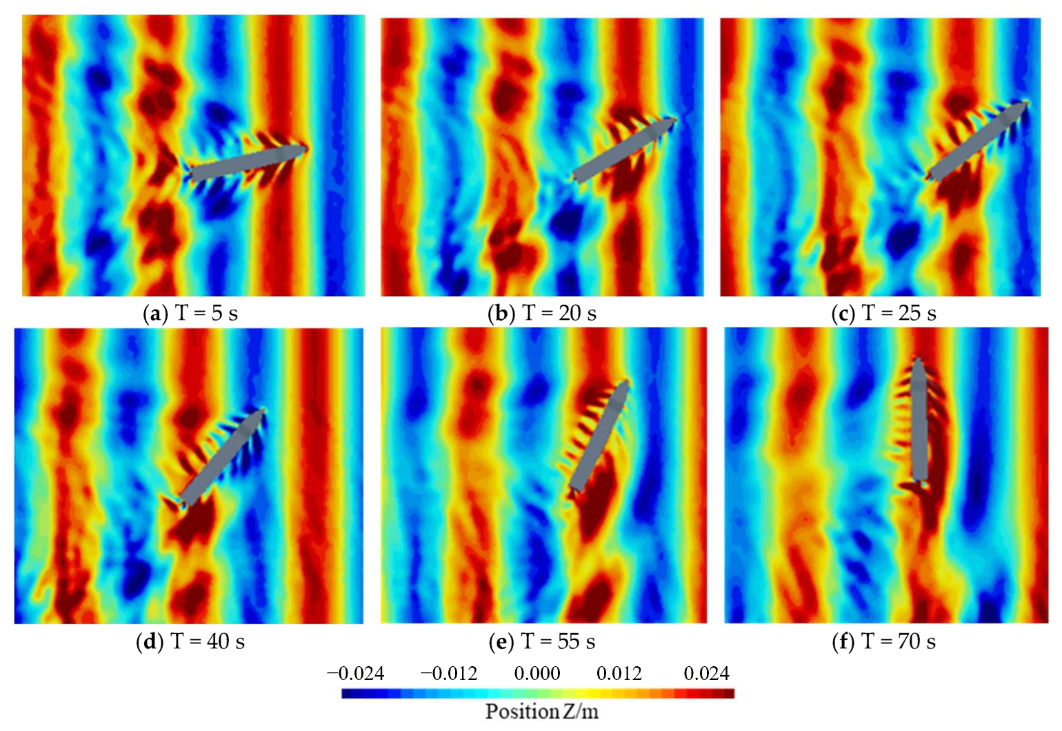
Figure 14 shows how the incident waves and ship-generated waves change during the turn. At t = 5 s, the ship is still close to its initial heading, and the wake is almost aligned with the original course. As the heading changes from t = 20 to 40 s, the wave encounter direction also changes, and the free surface pattern becomes less symmetric. At later times, the lower forward speed weakens the ship-generated waves, while the incident waves can still be seen around the hull. The sequence therefore shows the combined effects of heading change, speed loss, and wave encounter during the maneuver.

5. Conclusions

This study numerically investigated the self-propelled maneuvering of the KCS in regular waves. The principal quantitative conclusions are summarized as follows.

(1) Wave heading partitions the excitation among different response channels. Following seas (β = 0°) produce the largest reported resistance variation (51.99 N) and a pitch amplitude of 0.376°, while bow-quartering seas (β = 225°) produce a nearly identical pitch amplitude of 0.378°. Beam seas (β = 270°) reduce the corresponding resistance variation and pitch to 6.27 N and 0.068° but increase heave to 0.0150 m. The physical effect of heading is therefore a redistribution between longitudinal load/pitch excitation and vertical response, not a uniform loss of performance.

(2) The rudder-angle effect is strongly non-proportional. Increasing δ from 17.5° to 22.5° shortens advance by 39.7%, transfer by 40.5%, and tactical diameter by 36.5%, but the transient roll-growth slope rises by about 169%, from 0.013°/s to 0.035°/s. Tighter turning is therefore obtained at a disproportionately larger heeling penalty; calm-water turning indices alone do not represent the stability cost of aggressive steering in waves.

(3) The small heave-amplitude change of 0.0035 m across the same rudder range, together with the much larger roll-slope change and the stronger speed/thrust fluctuations at δ = 22.5°, separates the governing mechanisms. Rudder input mainly amplifies lateral acceleration, turning-induced heel, and propeller–rudder inflow unsteadiness, whereas heave remains controlled primarily by the incident-wave field.

(4) The free-surface sequence demonstrates that maneuvering loads are path-dependent. Yaw changes the instantaneous wave-encounter direction, while speed loss changes encounter frequency, so roll and thrust transients reflect the combined history of trajectory, rudder command, and wave phase. Wave-aware control should therefore coordinate steering with the evolving encounter condition rather than using only the initial heading.

Taken together, the results identify two distinct control variables: the imposed wave heading determines how excitation is partitioned among streamwise load, pitch, and heave, whereas the rudder angle determines the balance between path compactness and lateral/heeling-propulsion transients. The geometry-resolved propeller formulation allows these time-varying propulsion loads to be examined together with the free-running trajectory and ship motions, rather than inferring wave-maneuvering safety from calm-water indices alone.

The present conclusions are limited to the simulated regular-wave amplitude, wavelength, three headings, and rudder range; the reported roll slopes describe finite transient intervals rather than steady amplitudes. A controlled paired comparison between geometry-resolved MRF and virtual-disk propeller models was not performed, so the study does not claim the general superiority of one propulsion representation. Future work should repeat matched cases in irregular seas and at additional headings; compare overshoot angles, yaw rates, turning indices, motion and thrust spectra, and computational costs; and use time-accurate blade rotation plus experimental or full-scale validation to resolve transient blade loads.

References

- International Maritime Organization (IMO). 2023 IMO Strategy on Reduction of GHG Emissions from Ships; IMO: London, UK, 2023. [Google Scholar]
- International Maritime Organization (IMO). MSC.1/Circ.1595: E-Navigation Strategy Implementation Plan—Update 1; IMO: London, UK, 2018. [Google Scholar]
- International Maritime Organization (IMO). Autonomous Shipping; IMO: London, UK, 2025. [Google Scholar]
- The Specialist Committee on Manoeuvring in Waves. Final Report and Recommendations to the 29th ITTC. In Proceedings of the 29th International Towing Tank Conference, Virtual, 13–18 June 2021. [Google Scholar]
- Hamamoto, M.; Kim, Y.S. A new coordinate system and the equations describing manoeuvring motion of a ship in waves. J. Soc. Nav. Archit. Jpn. 1993, 1993, 209–220. [Google Scholar] [CrossRef] [Scilit]
- Skejic, R.; Faltinsen, O.M. A unified seakeeping and maneuvering analysis of ships in regular waves. J. Mar. Sci. Technol. 2008, 13, 371–394. [Google Scholar] [CrossRef] [Scilit]
- Yasukawa, H.; Yoshimura, Y. Introduction of MMG standard method for ship maneuvering predictions. J. Mar. Sci. Technol. 2015, 20, 37–52. [Google Scholar] [CrossRef] [Scilit]
- Zhang, W.; Zou, Z. Time domain simulations of the wave-induced motions of ships in maneuvering condition. J. Mar. Sci. Technol. 2016, 21, 154–166. [Google Scholar] [CrossRef] [Scilit]
- Zhang, W.; Zou, Z.J.; Deng, D.H. A study on prediction of ship maneuvering in regular waves. Ocean Eng. 2017, 137, 367–381. [Google Scholar] [CrossRef] [Scilit]
- Li, M.; Yuan, Z.-M.; Tao, L. Wash waves generated by ship moving across a depth change. Ocean Eng. 2023, 275, 114073. [Google Scholar] [CrossRef] [Scilit]
- Li, M.; Yuan, Z.-M.; Bai, X.; Li, Y.; Cheng, Y.; Tao, L. Numerical Modelling of Wash Waves Generated by Ships Moving over An Uneven Bottom. China Ocean Eng. 2023, 37, 145–153. [Google Scholar] [CrossRef] [Scilit]
- Li, M.; Chen, Y.; Yuan, Z.-M.; Cheng, Y.; Tao, L. Interference effects on the upstream wave generated by the catamaran moving across a depth change. Ocean Eng. 2023, 287, 115939. [Google Scholar] [CrossRef] [Scilit]
- Shigunov, V.; El Moctar, O.; Papanikolaou, A.; Potthoff, R.; Liu, S. International benchmark study on numerical simulation methods for prediction of manoeuvrability of ships in waves. Ocean Eng. 2018, 165, 365–385. [Google Scholar] [CrossRef] [Scilit]
- Kim, D.J.; Yun, K.; Park, J.-Y.; Kim, Y.G. Experimental investigation on turning characteristics of KVLCC2 tanker in regular waves. Ocean Eng. 2019, 175, 197–206. [Google Scholar] [CrossRef] [Scilit]
- Hasnan, M.A.A.; Yasukawa, H.; Hirata, N.; Terada, D.; Matsuda, A. Study of ship turning in irregular waves. J. Mar. Sci. Technol. 2020, 25, 1024–1043. [Google Scholar] [CrossRef] [Scilit]
- Kim, D.J.; Yun, K.; Yeo, D.J.; Kim, Y.G. Initial and steady turning characteristics of KCS in regular waves. Appl. Ocean Res. 2020, 105, 102421. [Google Scholar] [CrossRef] [Scilit]
- Suzuki, R.; Ueno, M.; Tsukada, Y. Numerical simulation of 6-degrees-of-freedom motions for a manoeuvring ship in regular waves. Appl. Ocean Res. 2021, 113, 102732. [Google Scholar] [CrossRef] [Scilit]
- Yu, L.; Wang, S.; Ma, N.N. Study on wave-induced motions of a turning ship in regular and long-crest irregular waves. Ocean Eng. 2021, 225, 108807. [Google Scholar] [CrossRef] [Scilit]
- Bondarenko, O.; Kitagawa, Y. Development of detailed engine model for evaluation ship performance in waves by a self-propulsion model test. J. Mar. Sci. Technol. 2022, 27, 266–277. [Google Scholar] [CrossRef] [Scilit]
- Deng, G.; Queutey, P.; Wackers, J.; Visonneau, M.; Guilmineau, E.; Leroyer, A. Assessment of ship maneuvering simulation with different propeller models. J. Hydrodyn. 2022, 34, 422–433. [Google Scholar] [CrossRef] [Scilit]
- Yu, J.; Feng, D.; Liu, L.; Yao, C.; Wang, X. Assessments of propulsion models for free running surface ship turning circle simulations. Ocean Eng. 2022, 250, 110967. [Google Scholar] [CrossRef] [Scilit]
- Gong, J.; Li, Y.; Dai, K.; Fu, Z.; Hong, Z. Numerical simulation of ship manoeuvring by a hybrid method with propulsive factors in waves taken into account. Ocean Eng. 2022, 264, 112538. [Google Scholar] [CrossRef] [Scilit]
- Yu, J.; Yao, C.; Huang, J.; Dong, G.; Zhang, Z.; Feng, D. Assessment of Different Hybrid Methods for Simulations of Free Running Surface Ship Maneuvering in Waves. Appl. Ocean Res. 2023, 139, 103703. [Google Scholar] [CrossRef] [Scilit]
- Kim, D.; Song, S.; Tezdogan, T. Free running CFD simulations to investigate ship manoeuvrability in waves. Ocean Eng. 2021, 236, 109567. [Google Scholar] [CrossRef] [Scilit]
- Kim, D.; Tezdogan, T. CFD-based hydrodynamic analyses of ship course keeping control and turning performance in irregular waves. Ocean Eng. 2022, 248, 110808. [Google Scholar] [CrossRef] [Scilit]
- Chen, C.; Zou, L.; Zou, Z.; Guo, H. Assessment of CFD-Based Ship Maneuvering Predictions Using Different Propeller Modeling Methods. J. Mar. Sci. Eng. 2022, 10, 1131. [Google Scholar] [CrossRef] [Scilit]
- Aram, S.; Mucha, P. CFD validation and analysis of turning maneuvers of a surface combatant in regular waves. Ocean Eng. 2024, 293, 116653. [Google Scholar] [CrossRef] [Scilit]
- Kim, B.-S.; Wang, S.; Zhu, Z.; Kim, Y. Numerical simulation of free-running turning test of ship in waves. Ocean Eng. 2023, 288, 115951. [Google Scholar] [CrossRef] [Scilit]
- Yasukawa, H.; Hirata, N. Effects of wave direction on ship turning in regular waves. Ocean Eng. 2023, 286, 115581. [Google Scholar] [CrossRef] [Scilit]
- International Towing Tank Conference (ITTC). Uncertainty Analysis in CFD, Verification and Validation Methodology and Procedures. ITTC Recommended Procedures and Guidelines 7.5-03-01-01, Revision 05, 2024. Available online: https://ittc.info/media/11718/0_0.pdf (accessed on 7 September 2026).
- Jessup, S.D. An Experimental Investigation of Viscous Aspects of Propeller Blade Flow Experiments; The Catholic University of America: Washington, DC, USA, 1989. [Google Scholar]
- SIMMAN2020. Workshop on Verification and Validation of Ship Manoeuvring Simulation Methods. Available online: https://simman2020.kr (accessed on 7 September 2026).
Figure 1.
KCS geometry with a rudder and a propeller.
Figure 2.
Mesh structure of the computational domain. (a) Top-view cross-section of the domain. (b) Midship cross-section of the domain. (c) Profile-view cross-section of the domain.
Figure 3.
Schematic of the (a) computational domain and (b) wave absorption zone.
Figure 4.
Grid resolutions used for the convergence assessment.
Figure 5.
Time-history curve of bow turning angular velocity under different time steps.
Figure 6.
Comparison of thrust coefficient, KT; scaled torque coefficient, 10KQ; and open-water efficiency, η0, at different advance ratios, J.
Figure 7.
(a) Zigzag trajectory in calm water. (b) Zigzag trajectory in wave conditions.
Figure 8.
Predicted turning trajectories of KCS: (a) calm water; (b) regular head waves.
Figure 9.
Time histories of (a) heave, (b) pitch, and (c) roll responses under different wave directions.
Figure 10.
Free-surface elevations for (a) calm water, (b) oblique waves, (c) following waves, and (d) beam waves.
Figure 11.
Turning trajectories with different δ values.
Figure 12.
Comparison of (a) roll motion and (b) heave motion under different rudder angles.
Figure 13.
Comparison of (a) ship-speed histories and (b) streamwise propeller-thrust histories at different rudder angles, δ.
Figure 14.
The free surface elevation during the turning maneuver at (a) 5 s, (b) 20 s, (c) 25 s, (d) 40 s, (e) 55 s, and (f) 70 s.