Modulations of Subsurface Circulation in a Shallow Marginal Sea by Extreme Typhoon Forcing, Revealing Hourly-Scale Transient Dynamics

Abstract

Typhoons can substantially perturb the thermal and circulation structure of marginal seas, yet in the Yellow Sea most studies have focused on surface cooling, vertical mixing, and coastal upwelling/downwelling, while the hourly-scale response of subsurface circulation below the thermocline remains poorly understood. Using the Finite Volume Community Ocean Model (FVCOM) combined with ERA5 reanalysis and satellite remote sensing, this study investigates the subsurface response of the South Yellow Sea during Typhoon Lekima (2019). Results reveal a pronounced transient sub-basin-scale anticyclonic circulation below the thermocline (30–70 m depth, maximum at 40–60 m) lasting approximately 15 h. This circulation exhibits significantly negative relative vorticity (O(10⁻⁵) s⁻¹) and coherent vertical structure, driven by barotropic pressure forcing. The barotropic sea surface height anomaly was traced to coastal wind forcing along the Shandong Peninsula and northern Jiangsu margins, which subsequently extended into the central basin. These findings reveal an overlooked pathway by which typhoons rapidly reorganize subsurface circulation in shelf seas, with implications for understanding the hourly-scale response of shelf seas to intensifying typhoon activity.

1. Introduction

Over the past several decades, the response of the upper ocean to translating typhoons has been a central topic in physical oceanography. The three-dimensional oceanic response to typhoon passage generally involves the formation of a surface cold wake on the right-rear side of the typhoon track [1,2,3], enhanced vertical mixing in the surface and subsurface layers [4,5], and the generation and propagation of near-inertial internal waves [6,7,8,9,10,11]. In the Northern Hemisphere, stronger sea surface temperature cooling is usually observed to the right of the typhoon track, owing to wind–current resonance and enhanced vertical mixing. Early studies primarily focused on typhoon-induced changes in sea surface temperature. In recent years, however, increasing evidence has shown that typhoons can modify not only the upper-ocean thermal structure but also the temperature, salinity, and current structures in the subsurface and deeper layers [12,13]. In shallow shelf seas and marginal seas, where water depth is limited, stratification is strong, tides are energetic, and topography is complex, typhoon-induced three-dimensional ocean responses often exhibit pronounced regional variability and strongly unsteady characteristics [14,15,16,17].

The Yellow Sea, located between the Korean Peninsula and mainland China, is a mid-latitude semi-enclosed shallow shelf sea on the margin of the northwestern Pacific Ocean, with a mean depth of only approximately 44 m. It is frequently affected by typhoons during summer and autumn [18,19,20]. Under strong solar radiation and relatively weak wind forcing in summer, the Yellow Sea develops pronounced vertical stratification, with warm surface water overlying colder subsurface and bottom water. The cold water occupying the central trough of the Yellow Sea is generally referred to as the Yellow Sea Cold Water Mass (YSCWM) [21]. The YSCWM is a seasonal water mass that persists in the central trough of the Yellow Sea and is characterized by low temperature [21]. The Yellow Sea exhibits a distinct seasonal circulation pattern characterized by cyclonic gyres in winter and weak anticyclonic circulation in summer, with the YSCWM persisting in the central trough throughout the warm season [22,23]. It also constitutes an important component of the subsurface circulation system in the Yellow Sea and plays a significant role in regional ecosystem dynamics and physical oceanographic processes [24,25,26,27].

Previous studies have demonstrated that typhoons can substantially perturb the thermal structure of the Yellow Sea. Lee et al. [28] found that the widespread sea surface cooling observed in the Yellow Sea during the summer of 2011 was mainly associated with strong vertical mixing induced by Typhoon Muifa, through which cold subsurface water was mixed upward and cooled the surface layer. Yang et al. [29], based on in situ observations, examined the influence of Typhoon Damrey on the shallow waters of the Yellow Sea and showed that pronounced surface cooling occurred after typhoon passage, while coastal downwelling and enhanced mixing jointly disturbed the cold bottom water. Yu et al. [30] combined observations with FVCOM numerical simulations to investigate the dramatic changes in bottom temperature along the coast of the northern Yellow Sea during Typhoon Lekima. They found significant bottom-temperature anomalies on both the northern side of the Shandong Peninsula and the southern side of the Liaodong Peninsula, indicating that even short-lived atmospheric forcing can induce substantial thermal responses in subsurface and bottom waters under conditions of strong stratification and complex topography.

In recent years, studies of typhoon-induced responses in the Yellow Sea have gradually extended from surface thermal effects to three-dimensional circulation and dynamical processes over daily to multi-day timescales [29,30,31,32,33,34,35,36]. Liu et al. [14] showed that, during Typhoon Lekima, the onshore surface flow near the Shandong Peninsula, coastal downwelling, and offshore bottom flow jointly formed a cross-shelf overturning circulation system in the northern Yellow Sea. Liu et al. [15] further demonstrated that Super Typhoon Bavi caused pronounced three-dimensional changes in temperature and currents in the Yellow Sea, characterized by surface cooling, subsurface warming, and displacement of cold water in the middle and lower layers. Ma et al. [37] emphasized that bottom topography, coastline geometry, and the relative position of the typhoon track with respect to the topography are key factors controlling the three-dimensional response of temperature and current fields in the Yellow Sea. The characteristics of the ocean response depend not only on storm intensity but also on translation speed, which sets the local forcing duration relative to the inertial period and thereby controls the relative importance of transient versus quasi-equilibrium adjustment [38].

Although previous studies have greatly advanced our understanding of typhoon-induced responses in the Yellow Sea, the hourly-term response of subsurface circulation of the South Yellow Sea remains insufficiently understood. In particular, the generation, development, and decay of short-lived circulation structures below the thermocline can be smoothed out in daily averaged or low-temporal-resolution datasets.

Typhoon Lekima in August 2019 provides a representative case for addressing these issues. Lekima moved northward along the eastern coast of China and passed near the central basin of the South Yellow Sea after entering the region. The interaction between its strong wind forcing and the pre-existing summer stratification in the Yellow Sea could have induced rapid dynamical adjustment below the thermocline. Unlike previous studies that mainly focused on sea surface cooling, coastal upwelling or downwelling, or bottom-temperature anomalies at daily-scale, this study focuses on ocean response at the hourly-scale anticyclonic circulation that developed in the subsurface layer of the central South Yellow Sea during the passage of Typhoon Lekima.

To this end, this study uses high-resolution numerical simulations based on the Finite Volume Community Ocean Model (FVCOM), together with satellite remote sensing data and ERA5 reanalysis winds. The model performance is first evaluated using sea surface temperature and sea surface height data. The hourly-scale evolution of the subsurface current field in the South Yellow Sea during the passage of Typhoon Lekima is then examined, and the anomalous anticyclonic circulation is identified and tracked. Finally, momentum and vorticity budget diagnostics are conducted to investigate the mechanisms responsible for the formation and decay of this anomalous anticyclonic circulation. The study is designed to address the following scientific questions:

• Did a significant hourly-scale anomalous circulation develop below the thermocline in the central basin of the South Yellow Sea during the passage of Typhoon Lekima?
• What were the temporal evolution, spatial structure, and vertical characteristics of this anomalous circulation?
• What roles did the pressure gradient force (and its barotropic and baroclinic components), Coriolis force, local acceleration, and vortex stretching play in the formation and maintenance of this circulation?

This study aims to reveal the rapid response mechanism of subsurface circulation in a shallow shelf sea under strong atmospheric forcing, to improve our understanding of subsurface current adjustment under strong stratification, and to provide a reference for interpreting the three-dimensional unsteady response of marginal seas to extreme weather events.

2. Data and Methods

2.1. Typhoon Lekima

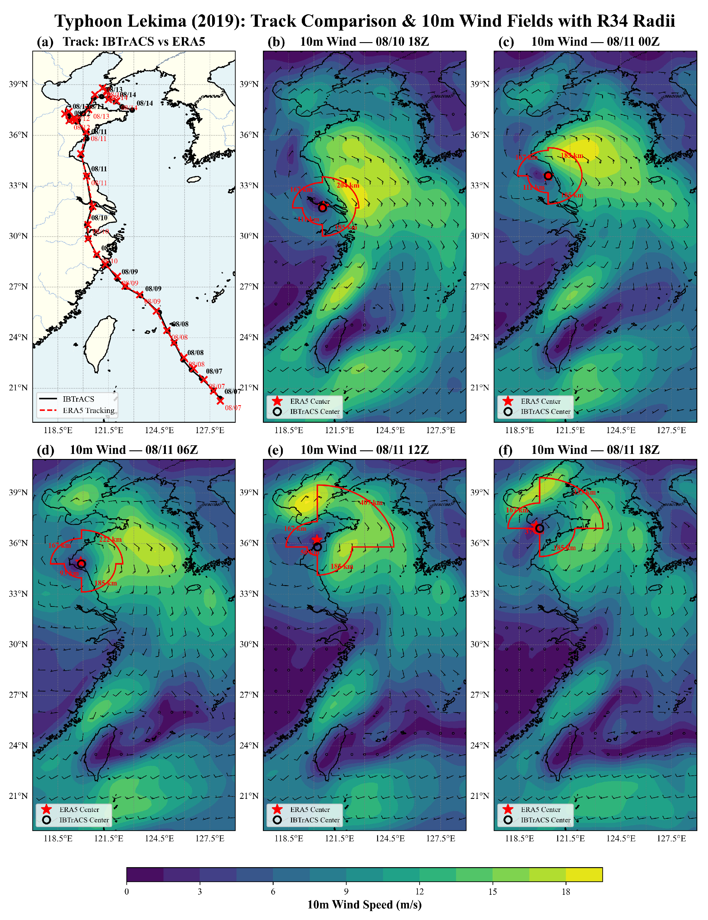
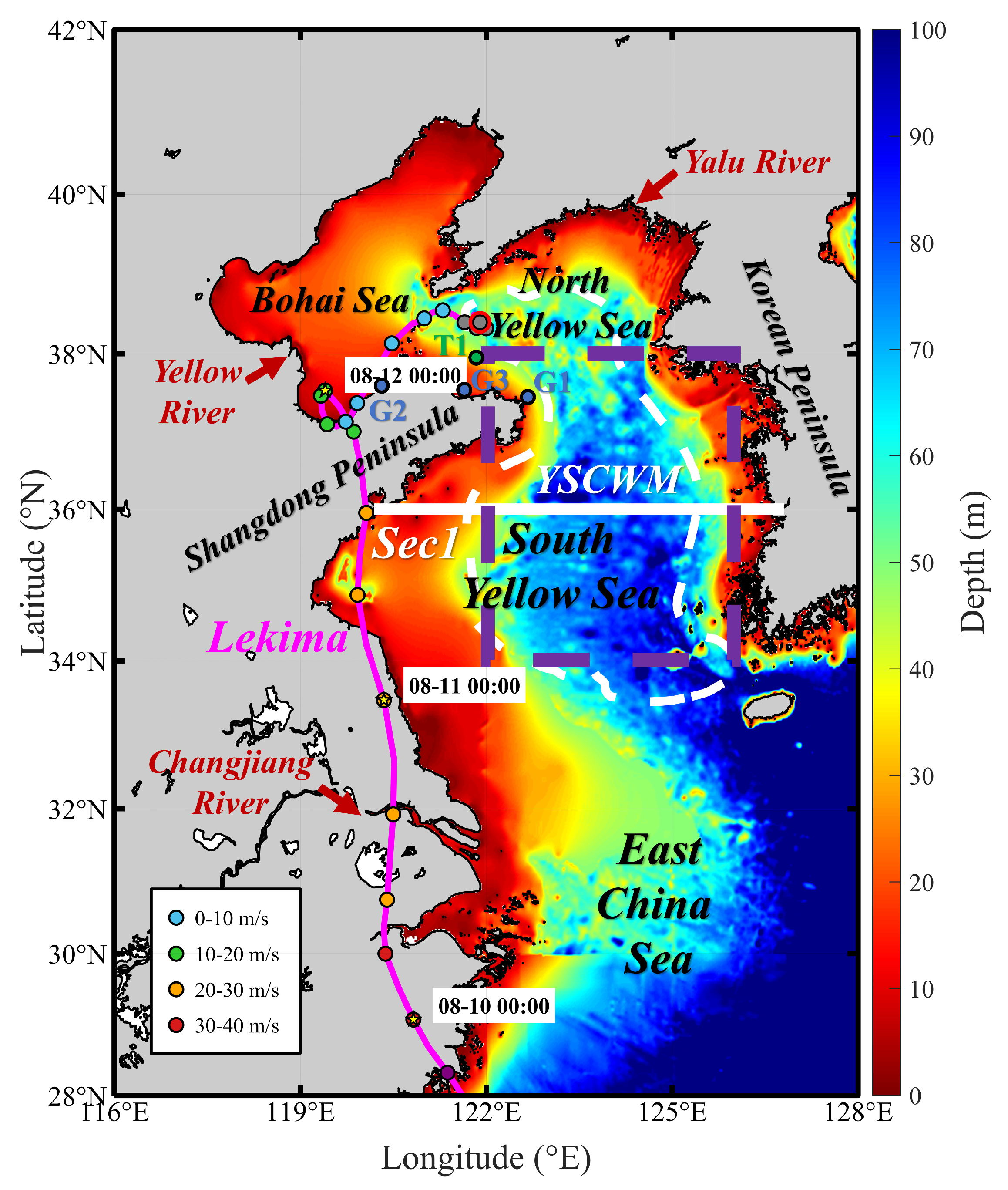
Typhoon Lekima, the ninth named typhoon of 2019, formed over the northwestern Pacific Ocean east of the Philippine Islands on 4 August 2019. On 9 August, Lekima passed over the East China Sea and made its first landfall in China over Zhejiang Province, with a maximum wind speed of approximately 52 m s⁻¹. At 12:00 on 11 August, Lekima entered the South Yellow Sea from the vicinity of Jiangsu Province and moved northward over the western South Yellow Sea. During the night of 11 August, the typhoon made landfall again over the Shandong Peninsula as a tropical storm, with a maximum wind speed of approximately 23 m s⁻¹. It then rapidly crossed the Shandong Peninsula and entered the Bohai Sea. By the morning of 13 August, Lekima had weakened into a tropical depression and eventually dissipated over the Bohai Sea. Typhoon Lekima track information was obtained from the China Meteorological Administration (CMA), while maximum wind speed and minimum central pressure were compiled from both the Japan Meteorological Agency (JMA) and CMA through the International Best Track Archive for Climate Stewardship (IBTrACS, doi:10.25921/82ty-9e16). The 6-hourly track data across the East China Sea, Yellow Sea, and Bohai Sea is shown in Figure 1. As IBTrACS data have been extensively used in previous typhoon-ocean interaction studies in the Yellow Sea region, these observations provided the reference dataset for ERA5 validation in this study [14,15,17,30].

2.2. Model Configuration

This study is primarily based on numerical simulations conducted using the Finite Volume Community Ocean Model (FVCOM [39,40]). The model domain covers the Bohai Sea, Yellow Sea, and East China Sea, spanning the geographic range of 21° N–41° N, 117° E–138° E (Figure S1). The computational grid consists of 70,479 nodes and 136,612 triangular cells. The horizontal resolution ranges from approximately 1–2 km in the coastal regions of the Bohai Sea and Yellow Sea, gradually coarsening to approximately 20 km toward the open ocean and open boundaries. In the vertical direction, a 30-layer sigma-coordinate system was employed. Bathymetric data were derived from the ETOPO1 global relief model, and were supplemented and refined with detailed water depth information from Chinese coastal nautical charts.

Atmospheric forcing at the sea surface was provided by the fifth-generation global coupled atmosphere–ocean–land reanalysis dataset (ERA5 [41]) produced by the European Centre for Medium-Range Weather Forecasts (ECMWF), including hourly fields of air temperature, sea-level pressure, 10 m winds, downward longwave and shortwave radiation, precipitation, evaporation, and relative humidity, at a spatial resolution of 0.25° × 0.25°. Open-boundary conditions, including sea surface height (SSH), horizontal velocity, temperature, and salinity, were derived from the GLORYS global ocean reanalysis product [42]. Tidal forcing was incorporated along the open boundaries by prescribing nine major tidal constituents (M₂, S₂, N₂, K₁, O₁, Q₁, M₄, MS₄, and MN₄) computed from TPXO7.2 [43], including both tidal elevation and barotropic tidal current components. Freshwater discharge from the four major rivers—the Yangtze River, Yellow River, Liao River, and Yalu River—was specified as lateral boundary inputs using daily streamflow records provided by the Water Resources Information Center of the Bureau of Hydrology, Ministry of Water Resources of China. Atmospheric forcing fields (ERA5) and open-boundary conditions (GLORYS, TPXO7.2) were interpolated from their native regular grids onto the FVCOM unstructured grid using bilinear interpolation [41,44]. The initial temperature and salinity fields were prescribed as the climatological mean derived from the GLORYS reanalysis [42]. The model was configured with external and internal time steps of 3 and 24 s, respectively. Starting from a cold-start initialization, the model was spun up for 13 years (1980–1992) to reach a quasi-steady state, then continued running from 1993 to 2024. Hourly model outputs from July 31 to August 31, 2019 were utilized for the analysis presented in this study. The FVCOM configuration employed in this study has been extensively validated against observational data in previous studies of typhoon-induced ocean responses in the Yellow Sea and adjacent seas [30,45,46,47,48].

2.3. Observational Data and Atmospheric Forcing

In situ observations used for model validation comprised a bottom-mounted temperature buoy and coastal tide-gauge records. A bottom-temperature buoy (station T1; 37.80° N, 121.90° E; local depth ~37 m) was deployed near the boundary of YSCWM in the coastal northern Yellow Sea. The buoy was equipped with an RBR Concerto temperature–salinity–depth profiler fixed approximately 0.4 m above the seafloor, with a nominal accuracy of ±0.002 °C and a sampling frequency of 1 Hz; hourly-averaged bottom-temperature records from 10 to 16 August 2019 were used to characterize the thermal response during Typhoon Lekima. Hourly sea-level observations were obtained from coastal tide-gauge stations G1 (39.24° N, 122.69° E), G3 (37.48° N, 121.48° E), and G2 (37.70° N, 120.36° E), located along the coast north of the Shandong Peninsula, covering the full month of August 2019. Sea levels at these stations were measured using float-type water-level gauges installed within tide-gauge wells, with monthly calibration against an external staff gauge. These records were used both to characterize the coastal sea-level response to typhoon forcing and to validate the model-simulated sea surface height fields.

Satellite-derived sea surface temperature (SST) data were used to evaluate the surface thermal response of the Yellow Sea during the passage of Typhoon Lekima. The SST product used in this study is the microwave/infrared optimum interpolated SST provided by Remote Sensing Systems (REMSS; https://www.remss.com). This product merges multi-source microwave and infrared satellite observations and can partly reduce the influence of cloud and rainfall contamination on infrared SST retrievals, making it particularly suitable for studies of SST responses to tropical cyclones. It has been widely adopted in SST studies of typhoon processes and demonstrated to provide reliable SST estimates under strong atmospheric forcing conditions [30,49,50].

SSH data used for model validation were obtained from the CMEMS (Copernicus Marine Environment Monitoring Service) satellite altimetry product. This satellite altimetry product has been widely used for ocean model validation in studies of typhoon-induced sea level and circulation responses in the northwestern Pacific and its marginal seas, and has been shown to provide reliable sea surface height estimates for evaluating model performance [14,15,16,37].

The 10 m wind fields used to force the model were obtained from the ERA5 reanalysis dataset produced by the European Centre for Medium-Range Weather Forecasts (ECMWF; [41]; https://cds.climate.copernicus.eu/ (accessed on 15 September 2024)). Prior studies have utilized the ERA5 dataset to investigate Typhoon Lekima [17,37]. Based on observations obtained by three buoys, Li et al. reported that the ERA5 dataset performed well in reproducing sea surface wind variations caused by Lekima in August 2019 and by Muifa in July 2011 [51]. These results confirm the feasibility of using ERA5 data to investigate typhoon-driven ocean responses.

2.4. Statistical Metrics

To quantitatively evaluate the performance of the FVCOM simulation, the model results were compared with satellite-derived SST and SSH observations using three complementary metrics: the root mean square error (RMSE), the temporal correlation coefficient (TCC), and the spatial correlation coefficient (SCC). These metrics characterize, respectively, the magnitude of the model–observation discrepancy, the consistency of the temporal evolution at each location, and the fidelity of the simulated spatial pattern at each instant.

Let $M_i$ and $O_i$ denote the simulated and observed values, respectively. The RMSE is defined as

$$\mathrm{RMSE}=\sqrt{{\displaystyle \frac{1}{N}}{\displaystyle \sum _{i=1}^N}{\left(M_i|-|O_i\right)}^2},$$

(1)

where $N$ is the number of samples. When the summation is performed over the time dimension at each grid point, the resulting field is referred to as the temporal RMSE; when it is performed over all grid points at each time step, it is referred to as the spatial RMSE.

The TCC is computed at each grid point as the Pearson correlation coefficient between the simulated and observed time series:

$$\mathrm{TCC}={\displaystyle \frac{{\displaystyle {\mathit{\sum }}_{\mathit{t}\mathit{=}\mathit{1}}^{{\mathit{N}}_{\mathit{t}}}}\left({\mathit{M}}_{\mathit{t}}\mathit{-}\overline{\mathit{M}}\right)\left({\mathit{O}}_{\mathit{t}}\mathit{-}\overline{\mathit{O}}\right)}{\sqrt{{\displaystyle {\mathit{\sum }}_{\mathit{t}\mathit{=}\mathit{1}}^{{\mathit{N}}_{\mathit{t}}}}{\left({\mathit{M}}_{\mathit{t}}\mathit{-}\overline{\mathit{M}}\right)}^{\mathit{2}}}\sqrt{{\displaystyle {\mathit{\sum }}_{\mathit{t}\mathit{=}\mathit{1}}^{{\mathit{N}}_{\mathit{t}}}}{\left({\mathit{O}}_{\mathit{t}}\mathit{-}\overline{\mathit{O}}\right)}^{\mathit{2}}}}}\mathit{,}$$

(2)

where $N_t$ is the number of time steps and $\overline{M}$ and $\overline{O}$ are the corresponding temporal means at that grid point. The TCC measures how well the model reproduces the observed temporal variability at each location.

The SCC is computed at each time step as the Pearson correlation coefficient over all grid points within the study region:

$$\mathrm{SCC}={\displaystyle \frac{{\displaystyle {\sum }_{k=1}^{N_s}}\left(M_k-\overline{M}\right)\left(O_k|-|\overline{O}\right)}{\sqrt{{\displaystyle {\sum }_{k=1}^{N_s}}{\left(M_k|-|\overline{M}\right)}^2}\sqrt{{\displaystyle {\sum }_{k=1}^{N_s}}{\left(O_k|-|\overline{O}\right)}^2}}},$$

(3)

where $N_s$ is the number of grid points and $\overline{M}$ and $\overline{O}$ are the corresponding spatial means at that time step. The SCC measures how well the model reproduces the observed spatial distribution at each instant. Together, these metrics provide a comprehensive assessment of model skill in both the temporal and spatial domains, and were applied to the SST and SSH validation presented in Section 3.1.

2.5. Identification, Boundary Definition, and Tracking of the Anomalous Circulation

The anomalous anticyclonic circulation was objectively identified and tracked at each hourly time step using a vector-geometry-based detection algorithm adapted from Nencioli et al. [52]. A candidate grid point was classified as the circulation center if it simultaneously satisfied four criteria: (1) meridional velocity (v) reversed sign across the point along the zonal direction and increased monotonically with distance; (2) zonal velocity (u) reversed sign along the meridional direction with monotonic increase; (3) local current speed was a local minimum within a 6-grid-point radius (~33.3 km), falling below the 1st percentile of domain-wide current speed while remaining non-zero; and (4) velocity vectors surrounding the point rotated coherently.

Centers identified at consecutive hourly time steps were linked into trajectories using nearest-neighbor tracking with a maximum separation threshold of 30 km and a minimum trajectory duration of 10 h to exclude spurious detections. At each time step, the radial extent of the circulation was determined by evaluating the four criteria at successively larger radii (6–50 grid points) until three consecutive radial increments failed the criteria. This objective procedure yielded reproducible definitions of the circulation’s center, spatial extent, and temporal continuity. The identified trajectories and radii were subsequently used to define the regions over which momentum and vorticity budget terms were spatially averaged.

2.6. Momentum Budget Analyses

The momentum budget analysis is based on the Navier–Stokes equations [53,54], which are decomposed into the eastward and northward momentum components as follows:

$${\displaystyle \frac{\partial u}{\partial t}}=-{\displaystyle \frac{1}{\rho }}{\displaystyle \frac{\partial p}{\partial x}}-\left(u{\displaystyle \frac{\partial u}{\partial x}}+v{\displaystyle \frac{\partial u}{\partial y}}+w{\displaystyle \frac{\partial u}{\partial z}}\right)+fv+{\displaystyle \frac{\partial }{\partial x}}\left(A_h{\displaystyle \frac{\partial u}{\partial x}}\right)+{\displaystyle \frac{\partial }{\partial y}}\left(A_h{\displaystyle \frac{\partial u}{\partial y}}\right)+{\displaystyle \frac{\partial }{\partial z}}\left(A_z{\displaystyle \frac{\partial u}{\partial z}}\right)$$

(4)

$${\displaystyle \frac{\partial v}{\partial t}}=-{\displaystyle \frac{1}{\rho }}{\displaystyle \frac{\partial p}{\partial y}}-\left(u{\displaystyle \frac{\partial v}{\partial x}}+v{\displaystyle \frac{\partial v}{\partial y}}+w{\displaystyle \frac{\partial v}{\partial z}}\right)-fu+{\displaystyle \frac{\partial }{\partial x}}\left(A_h{\displaystyle \frac{\partial v}{\partial x}}\right)+{\displaystyle \frac{\partial }{\partial y}}\left(A_h{\displaystyle \frac{\partial v}{\partial y}}\right)+{\displaystyle \frac{\partial }{\partial z}}\left(A_z{\displaystyle \frac{\partial v}{\partial z}}\right)$$

(5)

Here, $u$ and $v$ are the eastward and northward velocity components, respectively. The $x$, $y$, and $z$ directions are positive eastward, northward, and upward. $p$ is pressure, $\rho$ is seawater density, $f$ is the Coriolis parameter, and $A_h$ and $A_z$ are the horizontal and vertical turbulent viscosity coefficients, respectively.

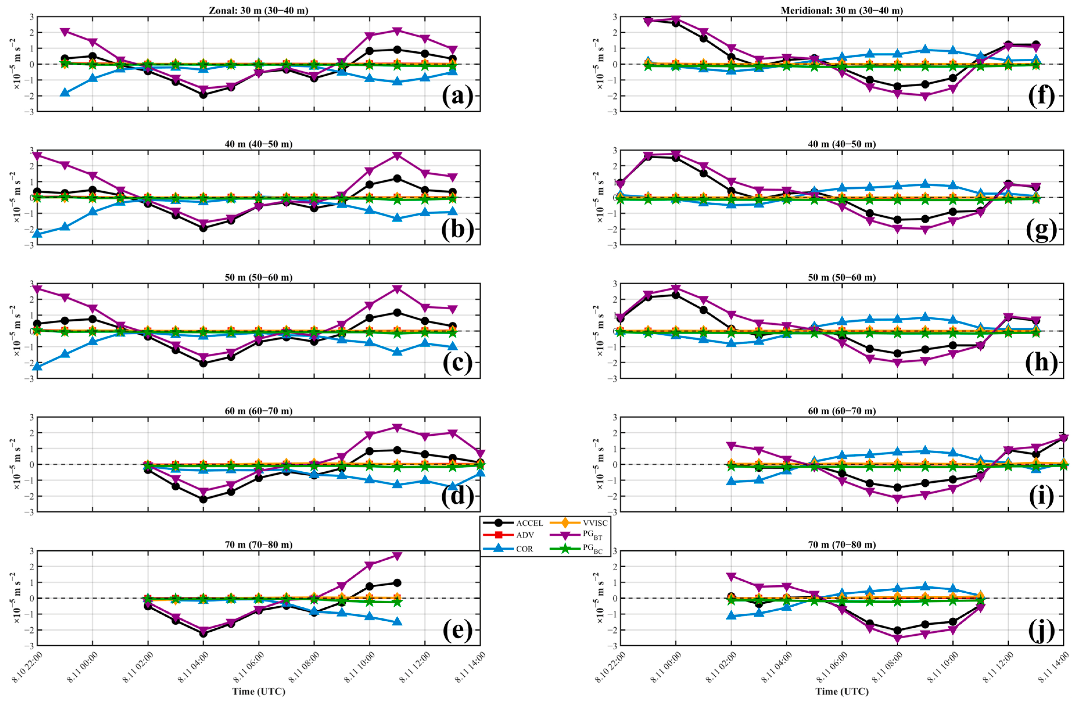
The term on the left-hand side denotes local acceleration and is referred to as ACCEL. The terms on the right-hand side represent the horizontal pressure gradient force (PG, including barotropic and baroclinic pressure gradient force), nonlinear horizontal advection (ADV), Coriolis force (COR), horizontal turbulent viscosity (HVISC), and vertical turbulent viscosity (VVISC), respectively. These budget terms were used to diagnose the dynamical balance associated with the formation and evolution of the anomalous anticyclonic circulation. Since the magnitude of HVISC was much smaller than that of the other terms, it is neglected in the subsequent analysis. The relative importance of the barotropic and baroclinic pressure gradient components was quantified using the ratio of the root mean square (RMS) residual magnitudes over the diagnosed period, and the closure of the momentum budget was evaluated as the RMS between the local acceleration term and the sum of the remaining terms, normalized by the mean magnitude of all budget terms.

Following the sigma-coordinate momentum equations solved by FVCOM, PG was separated into a barotropic component (PG_BT) and a baroclinic component (PG_BC) [55]. For the zonal direction,

$${PRSGRD}_x=\underset{{PG}_{BT}}{\underbrace{-gD{\displaystyle \frac{\partial \zeta }{\partial x}}}}\underset{{PG}_{BC}}{\underbrace{-{\displaystyle \frac{gD}{{\rho }_0}}\left[{\displaystyle \frac{\partial }{\partial x}}\left(D{\int }_{\sigma }^0\rho d{\sigma }^{\prime }\right)+\sigma \rho {\displaystyle \frac{\partial D}{\partial x}}\right]}},$$

(6)

and analogously for the meridional direction with $\partial /\partial y$. Here $\zeta$ is the sea surface elevation, $H$ the undisturbed water depth, $D=H+\zeta$ the total water column thickness, $\sigma =\left(z-\zeta \right)/D$ the terrain-following vertical coordinate, $\rho$ the density and ${\rho }_0$ a reference density. PG_BT is depth-independent and represents the contribution of the external (SSH) pressure field, whereas PG_BC depends on the vertical density structure and vanishes in a homogeneous water column.

To assess the sensitivity of the area-averaged momentum budget estimates to the choice of the circulation boundary, we performed a radius-perturbation sensitivity test in which the tracked radius at each depth and time step was scaled from −20% to +20% of its original estimate in increments of 5% (nine values in total). For each momentum term, the spatial average was recomputed for all nine radii, and the temporal-mean standard deviation across these nine estimates relative to the temporal-mean absolute value of the corresponding term was used as a coefficient-of-variation (CV) metric to quantify the relative uncertainty introduced by radius selection.

2.7. Vorticity Budget Analysis

To further investigate the dynamical mechanisms responsible for the development and maintenance of the circulation anomaly, a vorticity budget analysis was performed. The vorticity equation describes the evolution of fluid rotation, and quantitative evaluation of its individual terms allows the dominant physical processes controlling vorticity intensification or weakening to be identified. Based on the fundamental principles of fluid dynamics [53,54], the vertical vorticity equation can be written as

$$\begin{array}{c}{\displaystyle \frac{\partial \zeta }{dt}}+\left(u{\displaystyle \frac{\partial \zeta }{\partial x}}+v{\displaystyle \frac{\partial \zeta }{\partial y}}+w{\displaystyle \frac{\partial \zeta }{\partial z}}\right)+{\displaystyle \frac{df}{dt}}\\ =-\left(\zeta +f\right)\left({\displaystyle \frac{\partial u}{\partial x}}+{\displaystyle \frac{\partial v}{\partial y}}\right)+\left({\displaystyle \frac{\partial u}{\partial z}}{\displaystyle \frac{\partial w}{\partial y}}-{\displaystyle \frac{\partial v}{\partial z}}{\displaystyle \frac{\partial w}{\partial x}}\right)+{\displaystyle \frac{1}{{\rho }^2}}\left({\displaystyle \frac{\partial \rho }{\partial x}}{\displaystyle \frac{\partial p}{\partial y}}-{\displaystyle \frac{\partial \rho }{\partial y}}{\displaystyle \frac{\partial p}{\partial x}}\right)\\ +\left({\displaystyle \frac{\partial F_y}{\partial x}}-{\displaystyle \frac{\partial F_x}{\partial y}}{\displaystyle \frac{d\zeta }{dt}}\right)\end{array}$$

(7)

Here, $u$ and $v$ are the eastward and northward velocity components, respectively, and $w$ is the vertical velocity. The $x$, $y$, and $z$ axes are positive eastward, northward, and upward. $\rho$ is seawater density, $f$ is the Coriolis parameter, and $\zeta ={\displaystyle \frac{\partial v}{\partial x}}-{\displaystyle \frac{\partial u}{\partial y}}$ is the relative vorticity. The operator ${\displaystyle \frac{d}{dt}}$ denotes the material (Lagrangian) derivative.

The first and second terms on the left-hand side represent the material change in relative vorticity (RV) and planetary vorticity, or the $\beta$-effect (LV), respectively. The RV term can be further decomposed into two components: the local rate of change of relative vorticity (LCT) and the advection term (VA), which represents the advection of relative vorticity by the three-dimensional velocity field. The terms on the right-hand side represent different physical mechanisms affecting the vorticity tendency. The first term is the vortex stretching term (DT), which describes the effect of horizontal divergence on vertical vorticity. The second term is the tilting term (TT), representing the interaction between vertical shear and the horizontal gradient of vertical velocity. The third term is the baroclinic term (BT), which arises when isopycnal and isobaric surfaces are not aligned. The fourth term is the frictional term (FT), representing the effects of turbulent friction and subgrid-scale processes on vorticity, and was evaluated here as a residual term.

To assess the sensitivity of the area-averaged vorticity budget estimates to the choice of the circulation boundary, the same radius-perturbation sensitivity test described above (Section 2.6) was applied to each vorticity tendency term.

3. Results

3.1. Model Validation

3.1.1. In Situ Validation

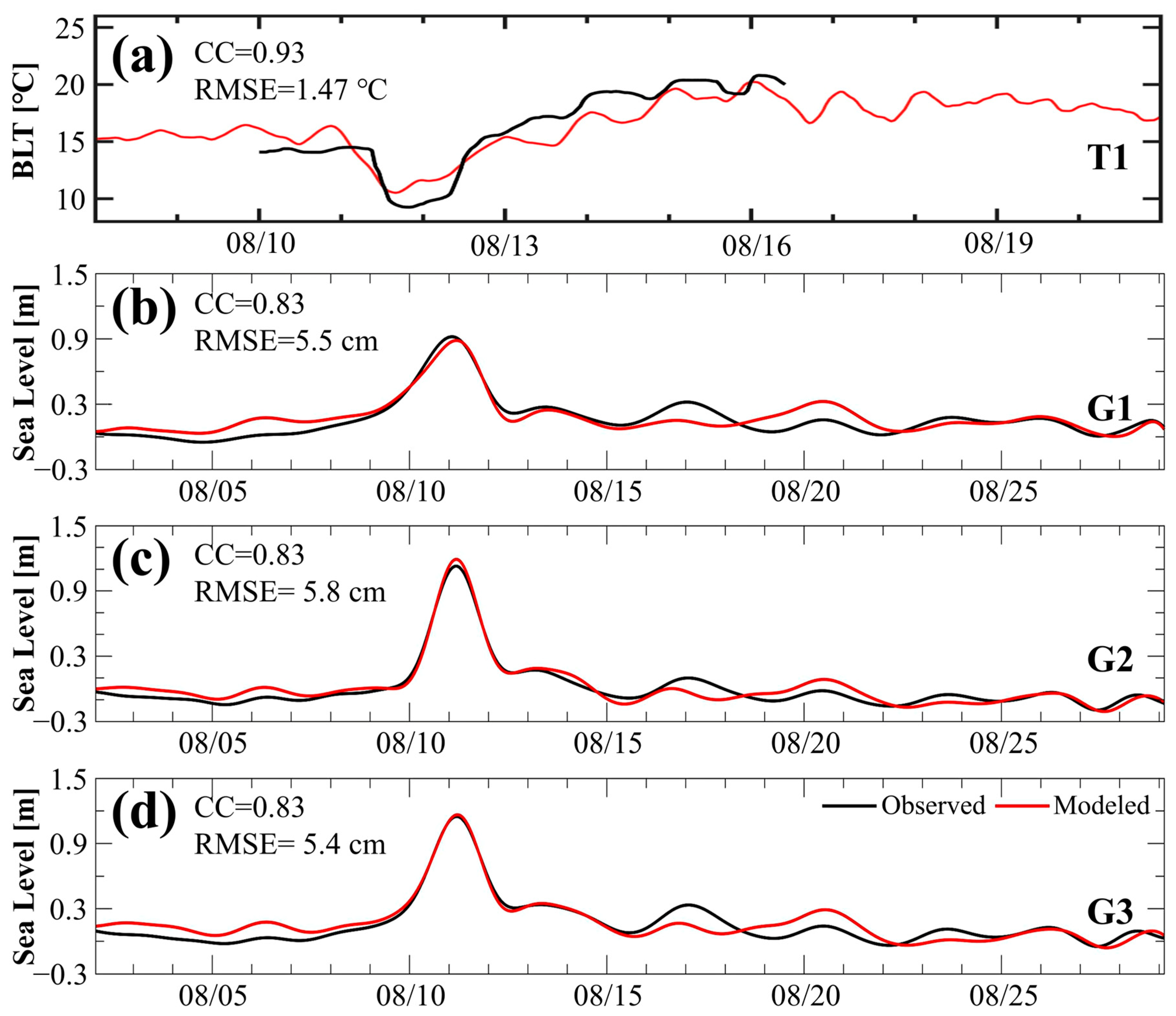
The model’s hourly-scale predictive skill was evaluated against mooring records and tide-gauge observations (Figure 1). The simulated bottom-layer temperature (BLT) at mooring T1 agreed well with observations (TCC = 0.93, RMSE = 1.47 °C; Figure 2a), correctly reproducing the ~5 °C abrupt cooling on 11–12 August and its recovery. A near-stationary warm bias of ~1 °C outside the typhoon period does not affect temporal evolution or pressure-gradient decomposition. Residual sea level was reproduced accurately at all three coastal stations (TCC = 0.83, RMSE = 5.4–5.8 cm; Figure 2b–d), with the storm surge peak (0.9–1.1 m on 11 August) captured within 5% amplitude and 1–2 h timing. All correlations were significant at the 95% level.

3.1.2. ERA5 Wind Field Validation

Using the IBTrACS best-track dataset as the observational benchmark, we systematically evaluated the reliability of the ERA5 reanalysis in reproducing the track and wind field of Typhoon Lekima (2019). Over the analysis period, the mean position error between the ERA5-derived track and the IBTrACS best track is approximately 23.7 km, which was smaller than the nominal horizontal grid spacing of ERA5 (~0.25°). During the over-ocean stage prior to landfall, the position errors remained largely within 20 km, and the two tracks nearly coincided (Figure 3a). Although the position error increased somewhat during the dissipating stage, when the system no longer maintained a coherent and well-defined circulation structure, ERA5 still reliably reproduced the overall storm translation.

Regarding the wind field during the period when the cyclone approached the coast, a comparison with the wind radii recorded in IBTrACS revealed a pronounced asymmetry: on the seaward side (northeastern quadrant), the area of enhanced 10 m wind speeds in ERA5 broadly corresponded to the observed wind circle, while on the landward side and in the near-core region, the ERA5 wind field is relatively weaker. This distribution was consistent with the track and structural evolution described above, indicating that the “strong-east–weak-west” asymmetric circulation of the typhoon is well captured (Figure 3b–f). Overall, ERA5 reliably reproduced both the synoptic-scale track over the open ocean and the asymmetric wind structure, thereby providing a sufficient atmospheric forcing basis for the ocean simulations conducted in this study.

3.1.3. SST Validation

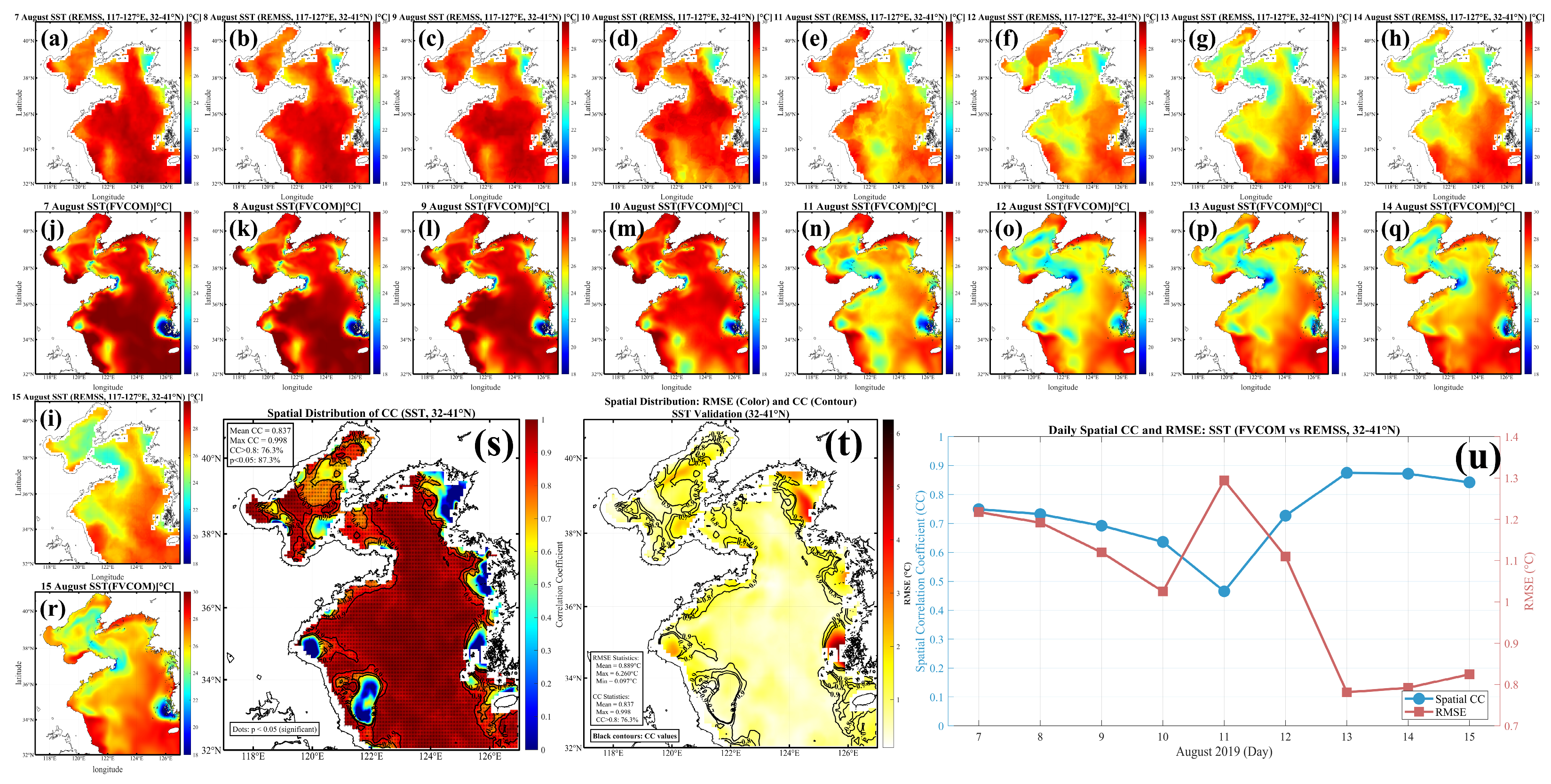
The sea surface temperature simulated by FVCOM agreed well with the REMSS satellite observations over the Bohai–Yellow Sea region from 7 to 15 August. In terms of spatial distribution, the simulated SST reproduced the major observed patterns, including the high-temperature region in the central South Yellow Sea before typhoon passage and the low-temperature regions north and south of the Shandong Peninsula after the typhoon passage. The simulation successfully captured the spatial heterogeneity of SST over the Bohai–Yellow Sea region, particularly the temperature contrast between the western and eastern Yellow Sea during the typhoon event (Figure 4a–r).

The TCC exceeded 0.9 over most of the study area, indicating good agreement between the simulated and satellite-observed temporal evolution of SST (Figure 4s). Relatively large temporal RMSEs were mainly found in the Bohai Sea, the western northern Yellow Sea, and the waters northeast of Shanghai (Figure 4t), possibly reflecting more complex nearshore dynamical processes in these regions. The daily SCC over the central South Yellow Sea remained high throughout the simulation period, while the spatial RMSE remained relatively stable and small (Figure 4u). The relatively lower SCC and elevated spatial RMSE on 11 August, coinciding with the typhoon’s passage, may be partly attributable to degraded satellite retrievals under severe weather conditions. Overall, the FVCOM model reproduced the observed SST patterns from 7 to 15 August 2019 with good agreement (Figure 4a–r), yielding a domain-averaged temporal correlation coefficient (TCC) of 0.837 (Figure 4s–u). All daily spatial correlation coefficients (SCCs), calculated from 87.3% of total 16,333 grid points per day, were statistically significant at p < 0.05.

3.1.4. SSH Validation

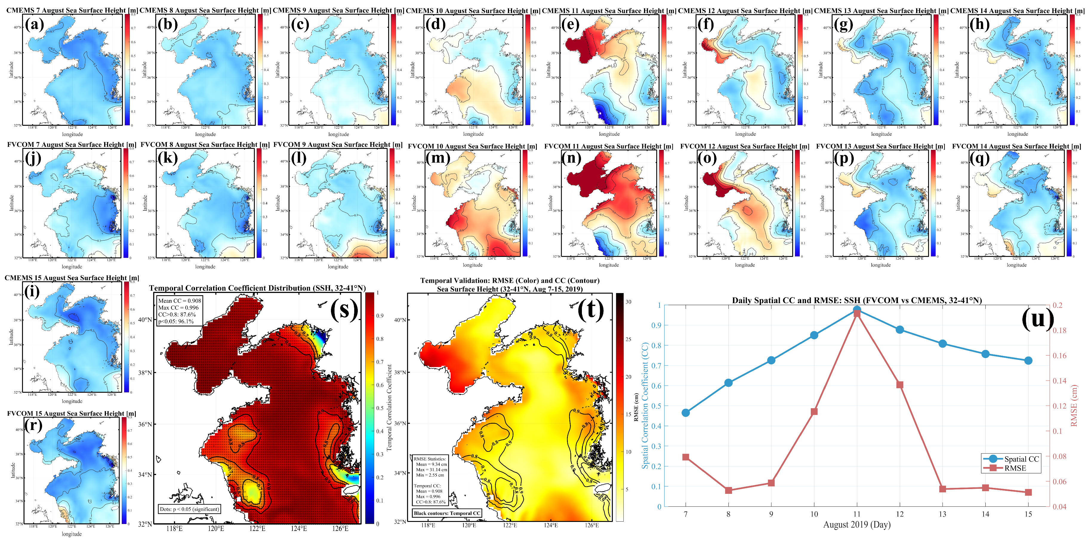
The sea surface height simulated by FVCOM was compared with CMEMS satellite altimetry observations over the Bohai–Yellow Sea region from 7 to 15 August. The simulated SSH distribution agreed well with the satellite observations, demonstrating that the model reasonably reproduced the spatiotemporal evolution of SSH in the study region (Figure 5a–r). The TCC exceeded 0.9 over most of the domain, suggesting a high degree of temporal consistency between the simulation and observations (Figure 5s). Temporal RMSE values were relatively uniform and small over the central Yellow Sea (Figure 5t). The SCC approached 1 during the typhoon passage on 11 August, although the spatial RMSE is also relatively large at this time, corresponding to the enhanced amplitude of SSH anomalies during the event (Figure 5u). Overall, the simulated SSH agreed well with CMEMS satellite altimetry over the Bohai–Yellow Sea region (Figure 5a–r), yielding a domain-averaged TCC of 0.908, with 96.2% of grid points passing significance at p < 0.05. All daily SCCs, calculated from 19,253 grid points per day, were statistically significant at p < 0.001, indicating robust model skill for the SSH field.

Overall, the validation results indicate that FVCOM reproduced the major spatiotemporal variability of the oceanic fields in the study area with good accuracy. However, it should be emphasized that Figure 4 and Figure 5 validate only the simulated surface thermal and sea-level response (SST and SSH). These comparisons do not directly verify the hourly-scale subsurface circulation, as no subsurface current observations were available. This limitation does not invalidate the model results: the hourly bottom-temperature record at T1 provides independent support for the subsurface thermal response (Figure 2a), and the subsurface dynamics are primarily driven by barotropic processes (sea surface height anomaly (SSHA) and vortex stretching) that are well-constrained by the validated SSH field. Therefore, the simulation provides a reliable basis for analyzing the subsurface response described in Section 3.3.

3.2. Current Field Evolution

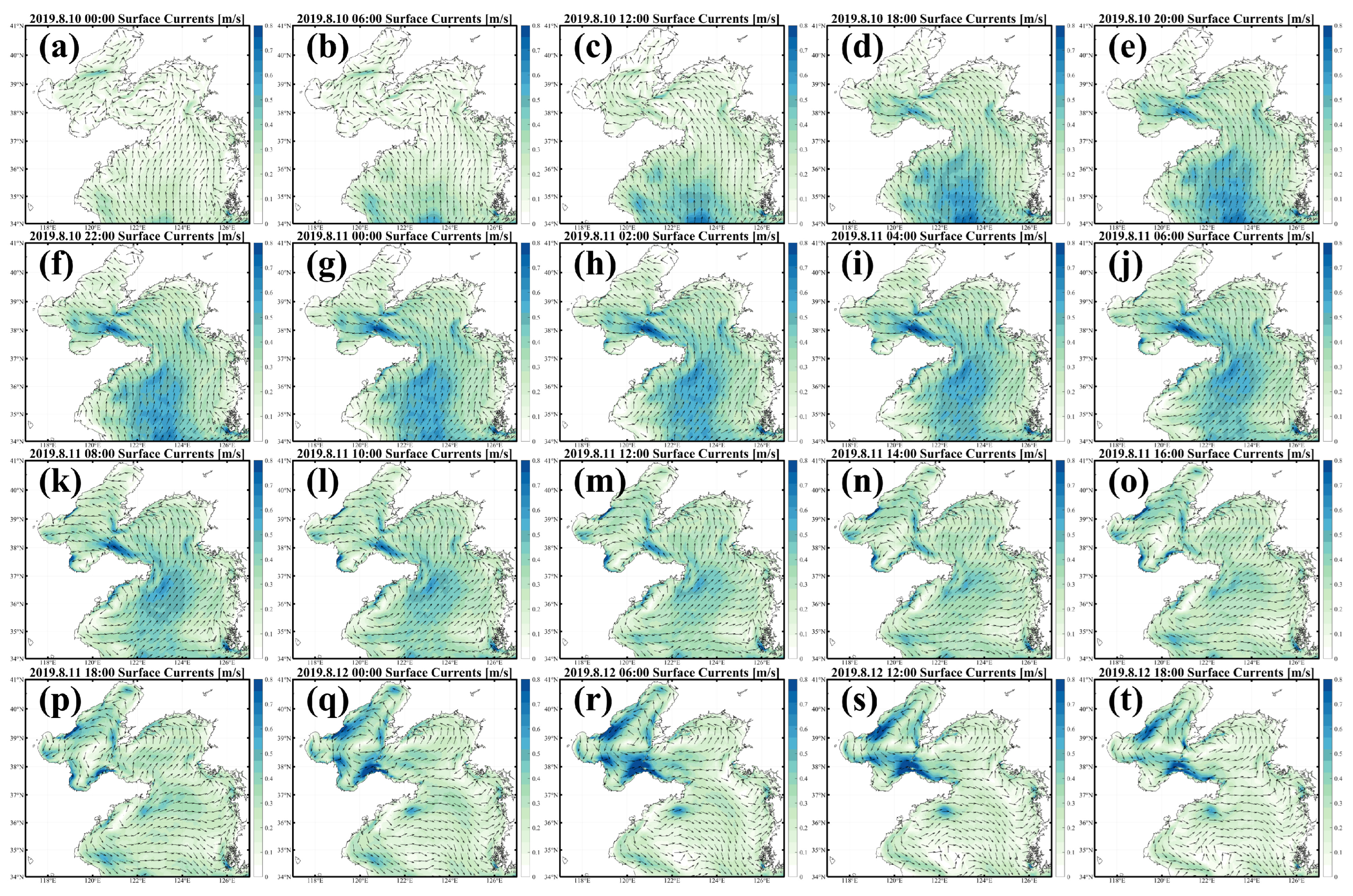
Hourly model output of current velocities, SSH, density fields, and the momentum and vorticity budget terms was low-pass filtered using a PL66 filter [56] with a 36 h cutoff period, to remove tidal and inertial fluctuations. Sensitivity experiments carried out with different cutoff periods (25, 30, 36, and 40 h) shown in Figure S2, confirmed the appearance of the anomalous circulation (Figures S3–S6). The surface circulation was primarily controlled by wind forcing, with the surface current direction generally oriented 45–90° to the right of the wind direction (Figure 6). Before the passage of Typhoon Lekima, the strong easterly winds associated with the approaching typhoon significantly enhanced surface currents in the Yellow Sea, especially over the central and western parts, and induced marked changes in flow direction. A strong surface current zone, with velocities of approximately 0.4–0.8 m s⁻¹, appeared ahead of the typhoon eye, and the South Yellow Sea was dominated by northward flow, while the northern Yellow Sea also began to shift toward northward flow (Figure 6a–i). As Typhoon Lekima moved northward, the region of strong surface currents migrated northward correspondingly. During the typhoon passage, the northern Yellow Sea was mainly characterized by northward flow, whereas the South Yellow Sea gradually shifted to northeastward and eastward flow; the strong surface current zone in the South Yellow Sea began to weaken and disappear (Figure 6j–m). After the typhoon passage, surface current speeds in the Yellow Sea decreased to less than 0.4 m s⁻¹. From 12 August onward, the surface circulation in the northern Yellow Sea exhibited a meridional contrast around 38°N: the northern part maintained northward flow, while the southern part shifted to southward and eastward flow, exporting water from the northern Yellow Sea into the South Yellow Sea. In the South Yellow Sea, the surface flow further turned eastward and then southeastward on 12 August, indicating that water transported into the Yellow Sea by the typhoon-induced strong wind forcing was rapidly exported from the region (Figure 6q–t).

Figure 6. Surface current fields in the Yellow Sea from 10 to 12 August 2019. (a–d) 00:00, 06:00, 12:00, and 18:00 on 10 August, at 6 h intervals; (e–p) 20:00 on 10 August to 16:00 on 11 August, at 2 h intervals; (q–t) 18:00 on 11 August to 18:00 on 12 August, at 6 h intervals (all times UTC). Current speed is indicated by color shading and current direction by black arrows. The current velocity data have been subjected to a 36 h low-pass filter.

Figure 6. Surface current fields in the Yellow Sea from 10 to 12 August 2019. (a–d) 00:00, 06:00, 12:00, and 18:00 on 10 August, at 6 h intervals; (e–p) 20:00 on 10 August to 16:00 on 11 August, at 2 h intervals; (q–t) 18:00 on 11 August to 18:00 on 12 August, at 6 h intervals (all times UTC). Current speed is indicated by color shading and current direction by black arrows. The current velocity data have been subjected to a 36 h low-pass filter.

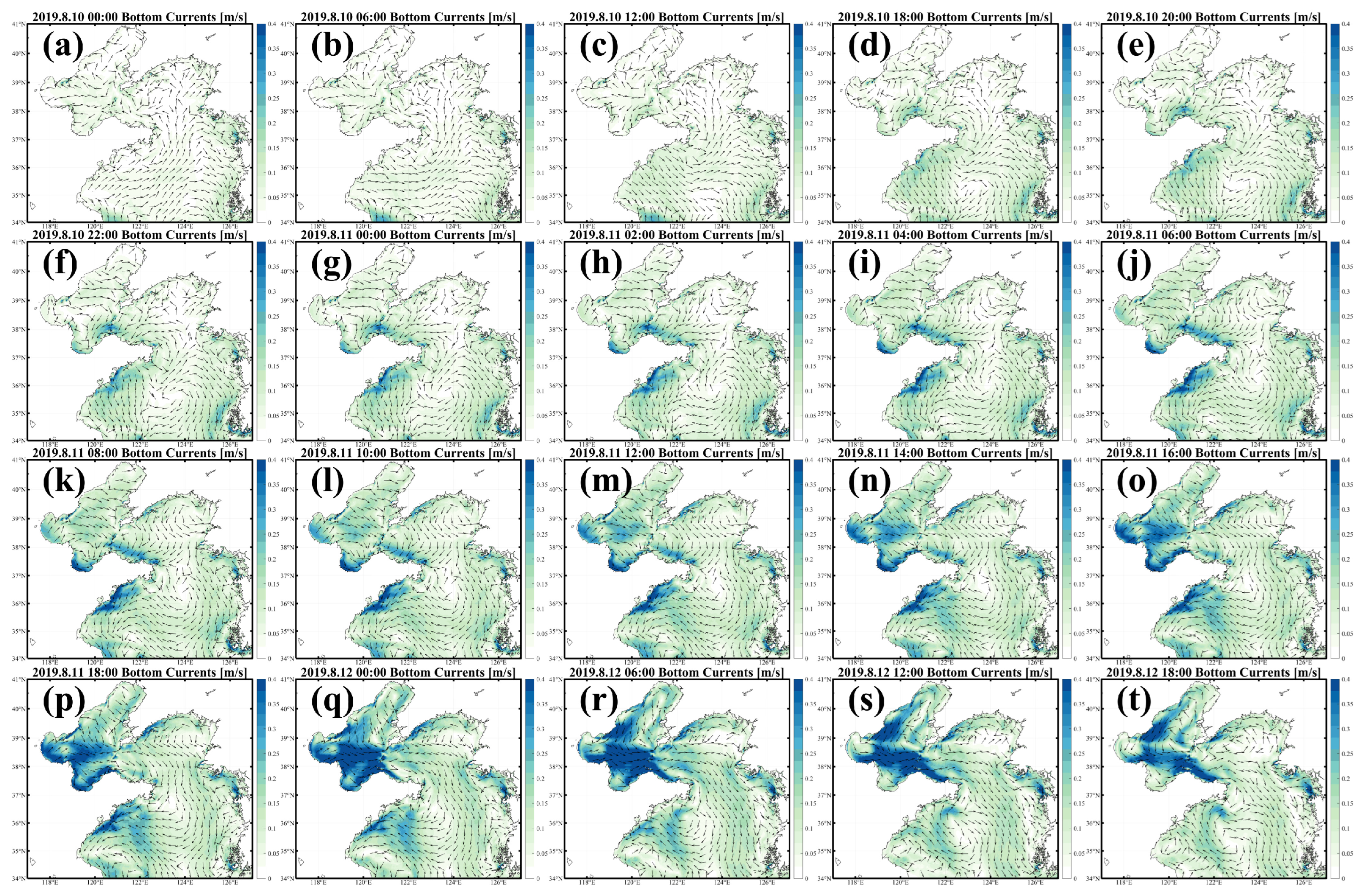
Before the typhoon passage, the bottom current field gradually intensified as Lekima approached, but its response lagged behind that of the surface layer. Bottom currents in the Yellow Sea were relatively weak from 00:00 to 12:00 on 10 August (Figure 7a–c). During 12:00–20:00 on 10 August, the surface circulation in the South Yellow Sea had already responded strongly to the approaching typhoon, whereas the bottom currents showed a clear east–west contrast separated approximately by 122° E. In the western South Yellow Sea, bottom currents were mainly southeastward, while in the eastern South Yellow Sea a low-velocity region developed between 122° E and 124° E, around which an anticyclonic circulation began to form (Figure 7c–e).

Additional current fields at 30 m and 50 m depths from 10 to 12 August show that the subsurface and bottom currents below the thermocline in the South Yellow Sea were generally consistent (Figures S5 and S7), indicating that the anticyclonic circulation existed throughout the middle and lower layers below the thermocline. The anticyclonic circulation migrated northward with the typhoon, with its center moving from approximately 35.5° N to 36.5° N between 00:00 and 12:00 on 11 August 2019. During the typhoon passage, the anticyclonic circulation became fully developed at 22:00 on 10 August; the flow on its western side turned westward and southward, while currents from the eastern and western sides converged near 122° E (Figure 7f). In the northern Yellow Sea, the bottom flow shifted to southward. After the typhoon passage at 12:00 on 11 August, bottom currents in the northern Yellow Sea remained southward, while the anticyclonic circulation in the central basin of the South Yellow Sea dissipated (Figure 7n–p). On 12 August, the South Yellow Sea exhibited a sub-basin-scale anticyclonic circulation pattern, with inflow on the western side and outflow on the eastern side (Figure 7q–t).

3.3. Anomalous Circulation Analysis

3.3.1. Characteristics of the Anomalous Circulation

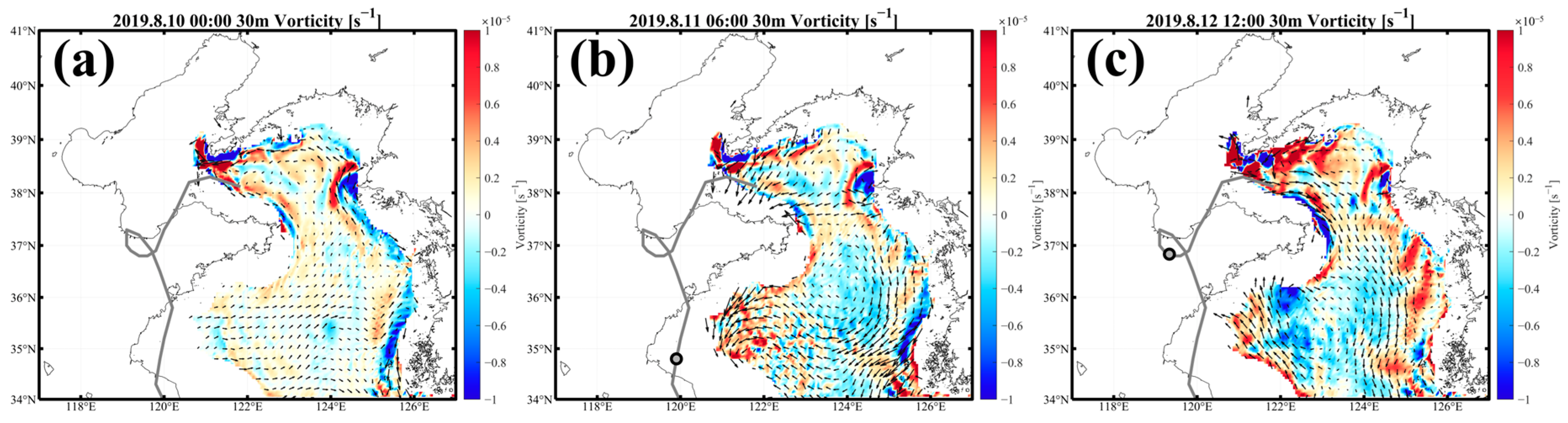
During the passage of Typhoon Lekima, a pronounced anomalous anticyclonic circulation developed in the central basin of the South Yellow Sea. To quantitatively characterize this transient event, the anomalous circulation was identified and tracked based on the current field and relative vorticity. During the development stage, the relative vorticity in the study region was significantly negative, with values of O(10⁻⁵ s⁻¹) at 30 m depth, clearly indicating the anticyclonic nature of the circulation. After the typhoon moved away, the negative vorticity anomaly rapidly dissipated (Figure 8a–c).

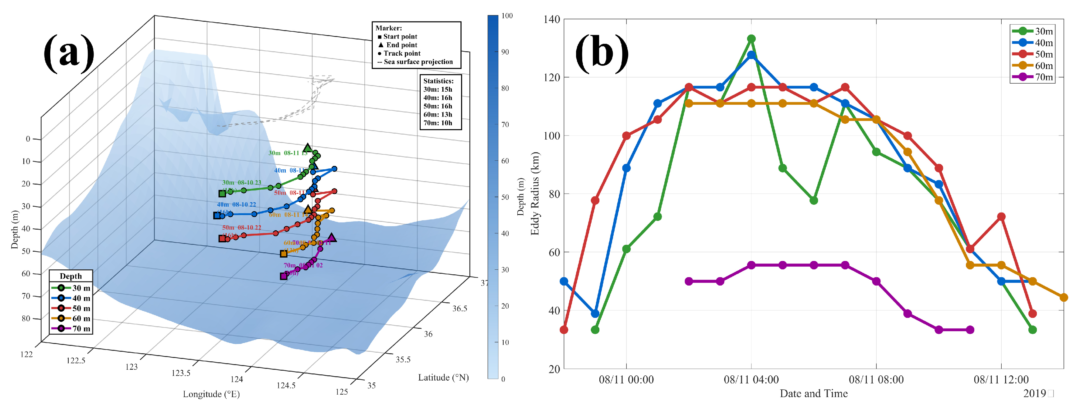
In terms of temporal evolution, the circulation exhibited a rapid generation–development–decay process, with a total duration of approximately 15 h (Figure 9a). It developed rapidly from the night of 10 August to the early morning of 11 August, reached its peak in the early morning of 11 August, persisted for approximately 6–8 h, and then rapidly weakened as the typhoon moved away. This timescale is shorter than the local inertial period of approximately 17 h, indicating that the circulation was a direct typhoon-forced response rather than a freely adjusted motion.

The generation, development, and decay of the circulation all occurred within approximately 15 h (Figure 9b), demonstrating a rapid response characteristic. During the development stage, from the night of 10 August to the early morning of 11 August, the circulation radius expanded rapidly at all depths. In particular, the radius at 40–60 m increased from approximately 40–80 km to 110–130 km, indicating that the mid-layer circulation structure was rapidly established. During the mature stage, approximately between 02:00 and 06:00, the mid-layer circulation maintained its maximum horizontal scale and varied only slightly. After the typhoon moved away, the circulation entered the decay stage, during which the radius decreased synchronously at all depths, indicating a coherent weakening of the whole circulation structure.

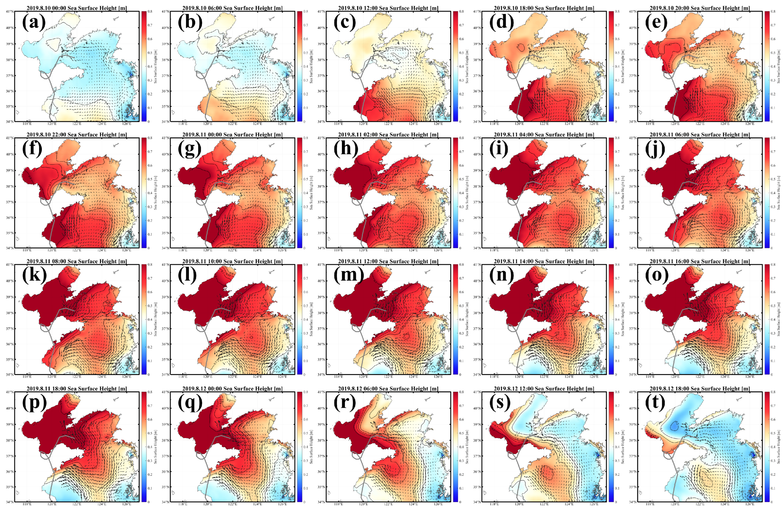
The vertical structure of the anomalous circulation exhibited clear stratified differences. The maximum horizontal scale was consistently located at 40–60 m depth, whereas the radius at 30 m showed stronger fluctuations and greater instability. At 70 m depth, the horizontal scale was significantly smaller, approximately 30–55 km. This indicated that the circulation was strongest in the middle layer and weaker above and below, further suggesting that it was not a typical surface wind-driven response but was more likely governed by the depth-dependent balance between local acceleration, frictional dissipation, and the barotropic pressure gradient force, as confirmed by the momentum budget analysis in Section 3.3.2. In addition, the radii at different depths varied coherently in time, especially during the development and decay stages, indicating that the circulation represented an integrated dynamical response. Combined with the SSH analysis (Figure 10), the circulation center corresponded well to a local SSH high anomaly, and the horizontal current field approximately satisfied geostrophic balance. However, significant deviations from geostrophy occurred during the rapid development stage, indicating a distinctly unsteady process. Further, we calculated the spatial Rossby number $R_o={\displaystyle \frac{\mathrm{U}}{\mathrm{f}\mathrm{L}}}$, which ranged from 0.009 to 0.012 across the 30–70 m layers. The temporal Rossby number $R_{o\mathrm{l}\mathrm{o}\mathrm{c}\mathrm{a}\mathrm{l}}={\displaystyle \frac{1}{\mathrm{f}\mathrm{T}}}$, was an order of magnitude larger (0.20–0.32), increasing systematically with depth from 0.22 at 30 m to 0.32 at 70 m, indicating the circulation retained a quasi-geostrophic spatial structure and was driven by a rapid, forced adjustment process.

To further characterize the nature of this anomalous circulation, the spatiotemporal evolution of SSH and 30 m currents in the Yellow Sea from 10 to 12 August 2019 was examined. During the formation and development of the anomalous anticyclonic circulation, the clockwise current structure at 30 m depth corresponded well to a local SSH high, indicating that the anomalous circulation had a clear pressure-field response. From the perspective of geostrophic adjustment, the horizontal pressure gradient around a positive SSHA in the Northern Hemisphere favors clockwise flow; this spatial correspondence between the SSH high and the anticyclonic current structure therefore provides important evidence for identifying the anticyclonic nature of the anomalous circulation (Figure 10).

It should be noted that the SSHA in Figure 10 mainly reflects the spatial correspondence between the anticyclonic circulation and the surface pressure field, and does not by itself establish the dynamical source of this pressure forcing. As shown by the momentum budget and pressure-gradient decomposition in Section 3.3.2, the barotropic pressure gradient force dominated the formation and maintenance of this circulation, indicating that the sub-basin-scale SSHA itself, rather than internal density restructuring, exerted the more direct dynamical influence on the subsurface flow. The SSH field in this section is therefore used primarily to describe the spatial structure and dynamical characteristics of the anomalous circulation, whereas its formation mechanism is further examined in Section 3.3.2.

3.3.2. Mechanisms of the Anomalous Circulation

The preceding section established, on the basis of the current field, relative vorticity, circulation center tracking, and SSH distribution, that a short-lived anomalous anticyclonic circulation formed below the thermocline in the central basin of the South Yellow Sea during the passage of Typhoon Lekima. The circulation exhibited a clear pressure-field signature corresponding to a local SSH high. However, the SSH distribution alone is insufficient to determine the specific source of the pressure forcing or to distinguish the relative roles of the barotropic and baroclinic pressure gradient forces in the adjustment of the subsurface current field. The following diagnostic analyses—encompassing momentum budget, vorticity budget, and temperature–density structure analyses—were therefore applied to elucidate the formation and maintenance mechanisms of the anomalous anticyclonic circulation.

Momentum budget. The temporal evolution of the zonal and meridional momentum budget terms for the anticyclonic circulation at depths of 30, 40, 50, 60, and 70 m from 22:00 on 10 August to 14:00 on 11 August 2019 is presented in Figure 9. The pressure gradient force (PG) and Coriolis force (COR) were dominant in magnitude throughout the diagnosed period. These two terms did not achieve a strict balance. The local acceleration term (ACCEL) remained non-negligible during the rapid development stage, and the circulation therefore evolved under a strongly unsteady adjustment state rather than quasi-steady geostrophic balance. Further decomposition of the pressure gradient force into barotropic and baroclinic components revealed that the barotropic component was substantially larger than the baroclinic component at all diagnosed depths (Figure 11), indicating that the pressure forcing of the subsurface circulation was primarily associated with the sub-basin-scale SSHA itself, rather than with rapid changes in the internal density structure of the water column. The RMS magnitudes of barotropic and baroclinic pressure gradient components (PG_BT/PG_BC) were calculated for each depth and momentum component (

Table 1. Representative barotropic-to-baroclinic pressure gradient ratios (PG_BT/PG_BC) and momentum budget closure residuals for the anomalous circulation-tracked region at each diagnosed depth layer (30–70 m) and momentum component (zonal u, meridional v), based on the area-averaged time series shown in Figure 11.

Depth (m)	Direction	PGBT/PGBC	Residual RMS (%)
30	u	19.22	0.09
	v	10.66	0.07
40	u	19.25	0.06
	v	10.21	0.09
50	u	16.13	0.03
	v	10.31	0.09
60	u	10.88	0.05
	v	8.83	0.07
70	u	11.30	0.08
	v	8.39	0.05

). The RMS ratios ranged from 8.39 to 19.25, confirming that barotropic pressure forcing was consistently about one order of magnitude larger than the baroclinic component. The momentum budget closure was verified with a residual RMS between 0.03% and 0.09% (Table 1). This result motivates an examination of the origin of the local SSH high in the central basin, which is presented in Section 3.3.3. A sensitivity scan of the tracking radius (±20%) was performed to evaluate the robustness of budget estimates. The main three momentum budget terms, ACCEL, COR and PG_BT terms, exhibited low coefficients of variation across all depths (0.024–0.113), indicating that budget estimates were insensitive to the precise choice of tracking radius. This uncertainty range is shown by the shaded envelope (±1 SD) in Figure S8.

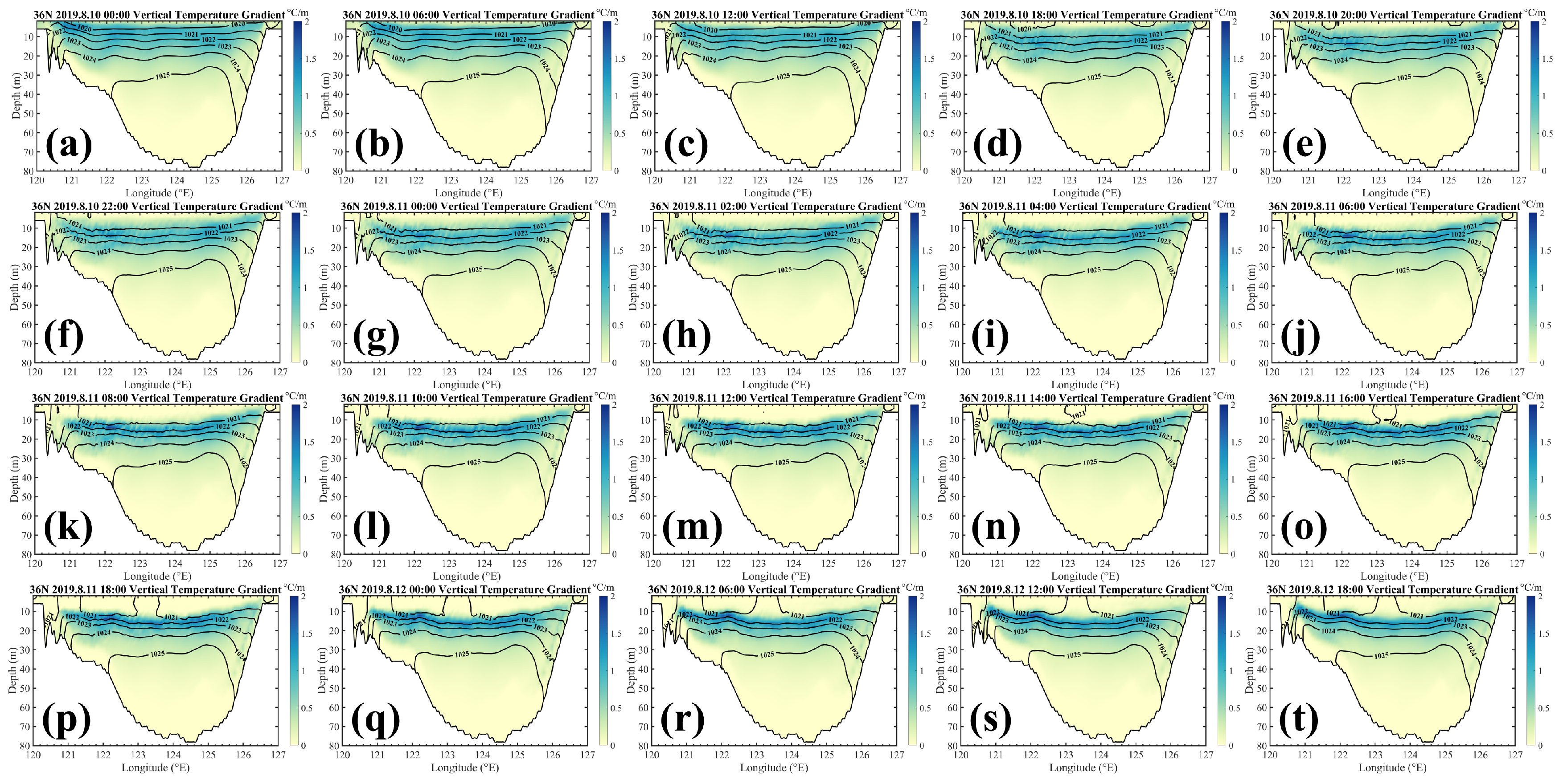
Temperature–density structure. The vertical temperature gradient and isopycnals along the zonal transect Sec1 (36° N) from 10 to 12 August 2019 exhibited the typical vertical structure of the YSCWM, with warm water and weak temperature gradients in the surface layer, a pronounced thermocline in the middle layer, and the cold YSCWM body near the bottom. During the typhoon passage, stratification in the central South Yellow Sea was disturbed, and the enhanced temperature gradient was mainly concentrated near the thermocline at approximately 20 m depth. No pronounced isopycnal tilting was observed within the main body of the cold water mass at 40–60 m. These structural features indicated that the enhanced density gradient was confined mainly to the thermocline near 20 m depth (Figure 12). It is worth noting that the thermocline thickening at ~20 m was distinct from the near-surface stratification expected from precipitation-induced freshening, consistent with Ma et al. [37] and Zhang et al. [57], who similarly attributed thermocline deepening in this region to wind-enhanced vertical mixing.

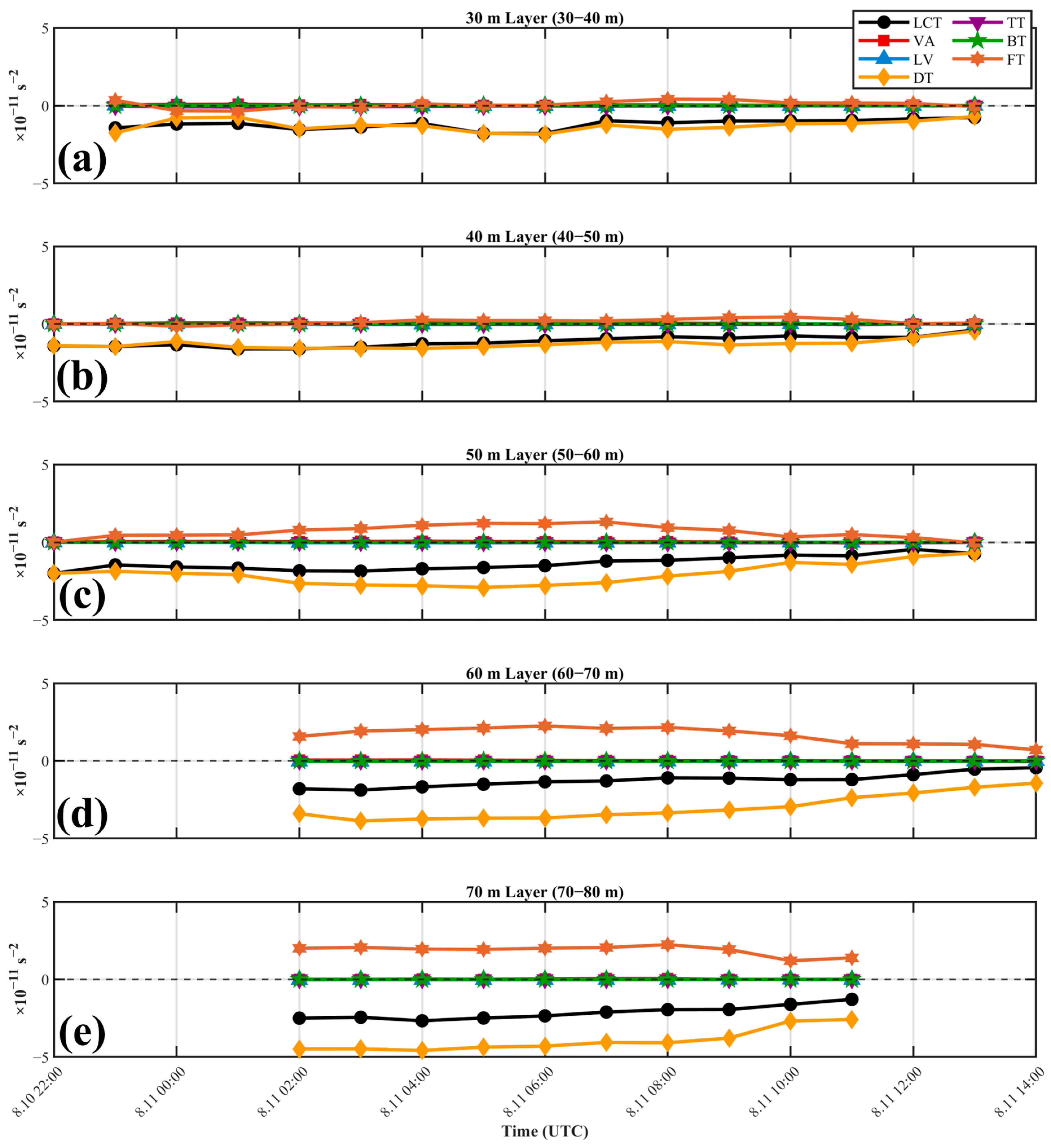
Vorticity budget. The temporal evolution of the vorticity budget terms for the anticyclonic circulation at depths of 30, 40, 50, 60, and 70 m from 22:00 on 10 August to 14:00 on 11 August 2019 showed consistent temporal variations across all depths throughout the diagnosed period. During the formation and maintenance stages of the anticyclonic circulation, the vortex stretching term was the dominant contributor to negative vorticity. In the Northern Hemisphere, when horizontal divergence occurs in the subsurface layer, the stretching term $-\left(f+\zeta \right){\mathit{\nabla }}_h\cdot \mathit{u}$ becomes negative, thereby promoting the generation of anticyclonic relative vorticity. During the development stage, the rate of negative vorticity generation by the stretching term exceeded the compensating effect of friction, allowing the local relative vorticity to remain significantly negative and sustaining the anticyclonic circulation structure (Figure 13). This result motivates an examination of the vorticity balance governing the circulation evolution, which is presented examined below. A sensitivity scan of the tracking radius (±20%) was performed to evaluate the robustness of budget estimates. The three main vorticity budget terms, FT, DT and LCT, exhibited low coefficients of variation across all depths (0.032–0.153), indicating that budget estimates are insensitive to the precise choice of tracking radius. This uncertainty range is shown by the shaded envelope (±1 SD) in Figure S9.

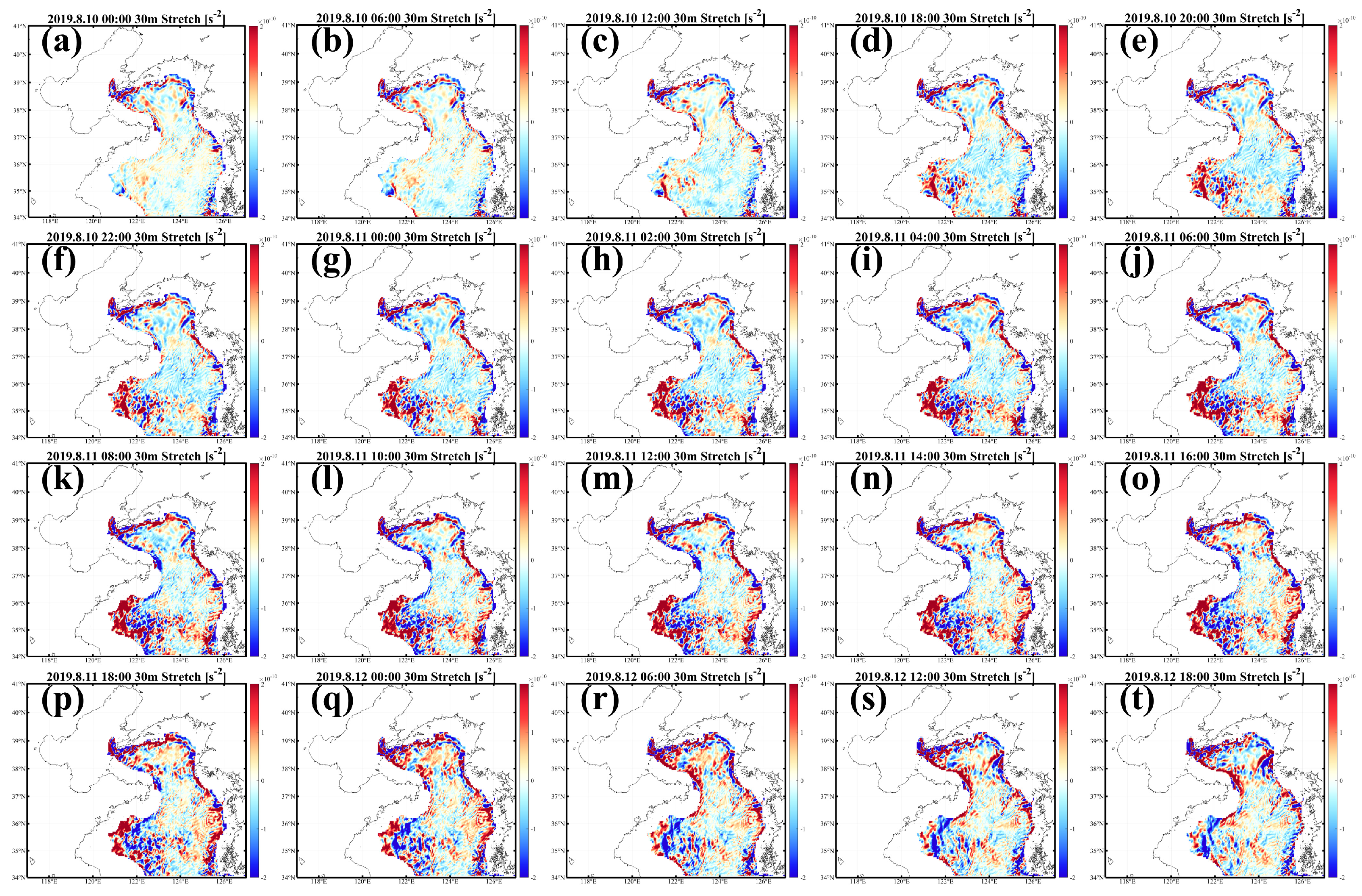
Vortex stretching tendency. Prior to the arrival of the typhoon (Figure 14a–d), the DT in the central South Yellow Sea was weak and spatially incoherent, with amplitudes generally below 0.5 × 10⁻⁹ s⁻². Between 22:00 on 10 August and 12:00 on 11 August (Figure 14f–m), coinciding with the formation and maturation of the anomalous anticyclonic circulation, a coherent patch of negative (anticyclone-generating) DT developed in the basin interior, with values reaching approximately −1 × 10⁻⁹ s⁻², i.e., one to two orders of magnitude larger than the pre-typhoon background. After 18:00 on 11 August (Figure 14p–t), the coherent interior signal disappeared and the field reverted to a coastally confined, small-scale pattern. The DT in the basin interior exhibited a southwest–northeast asymmetry, mirroring the dipole structure of the vertical velocity field at the same depth (upwelling to the southwest, downwelling to the northeast; Figure S10).

3.3.3. Coastal Ekman Forcing by Wind and Its Spatial Extension

The momentum budget analysis in Section 3.3.2 established that the barotropic pressure gradient force, rather than internal density restructuring, was the primary source of pressure forcing acting on the subsurface circulation. This result raises the question of how the local SSH high in the central basin was itself established. To address this, the wind stress curl-derived Ekman pumping field and its cumulative effect over the typhoon passage were diagnosed.

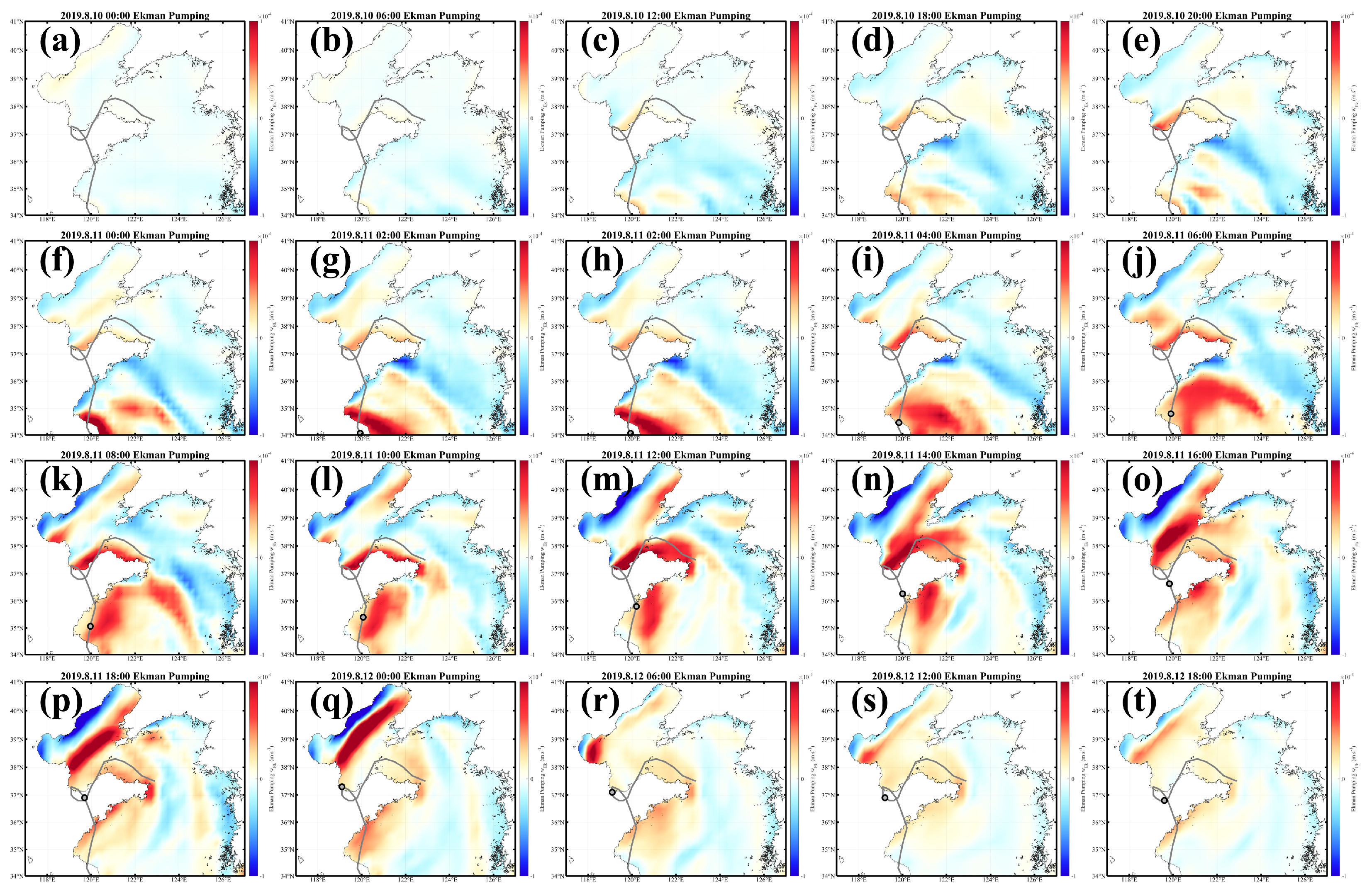
The instantaneous Ekman pumping field (Figure 15) shows that Ekman pumping remained weak throughout the basin during the early stage of the typhoon’s approach (Figure 15a–e). As the typhoon intensified and moved closer to the coast, distinct banded structures of strong Ekman pumping developed along the coastal margins of northern Jiangsu and the Shandong Peninsula (Figure 15f–j), reaching peak intensity between 08:00 and 16:00 on 11 August, when the typhoon center was located near the coast (Figure 15k–o). Throughout this period, Ekman pumping within the central basin, where the anomalous anticyclonic circulation subsequently developed, remained markedly weaker than along the coastal bands. As the typhoon moved northward and weakened, the strong Ekman pumping signal migrated northward and gradually decayed (Figure 15p–t).

Figure 15. (a–t) Ekman pumping velocity (color shading) at 30 m depth in the Yellow Sea from 10 to 12 August 2019, at the same time steps as Figure 6. Red (blue) shading indicates upward (downward) Ekman pumping associated with positive (negative) wind stress curl. The grey curve indicates the track of Typhoon Lekima, and the dot with a black outline and grey center marks the typhoon center position at the corresponding time.

Figure 15. (a–t) Ekman pumping velocity (color shading) at 30 m depth in the Yellow Sea from 10 to 12 August 2019, at the same time steps as Figure 6. Red (blue) shading indicates upward (downward) Ekman pumping associated with positive (negative) wind stress curl. The grey curve indicates the track of Typhoon Lekima, and the dot with a black outline and grey center marks the typhoon center position at the corresponding time.

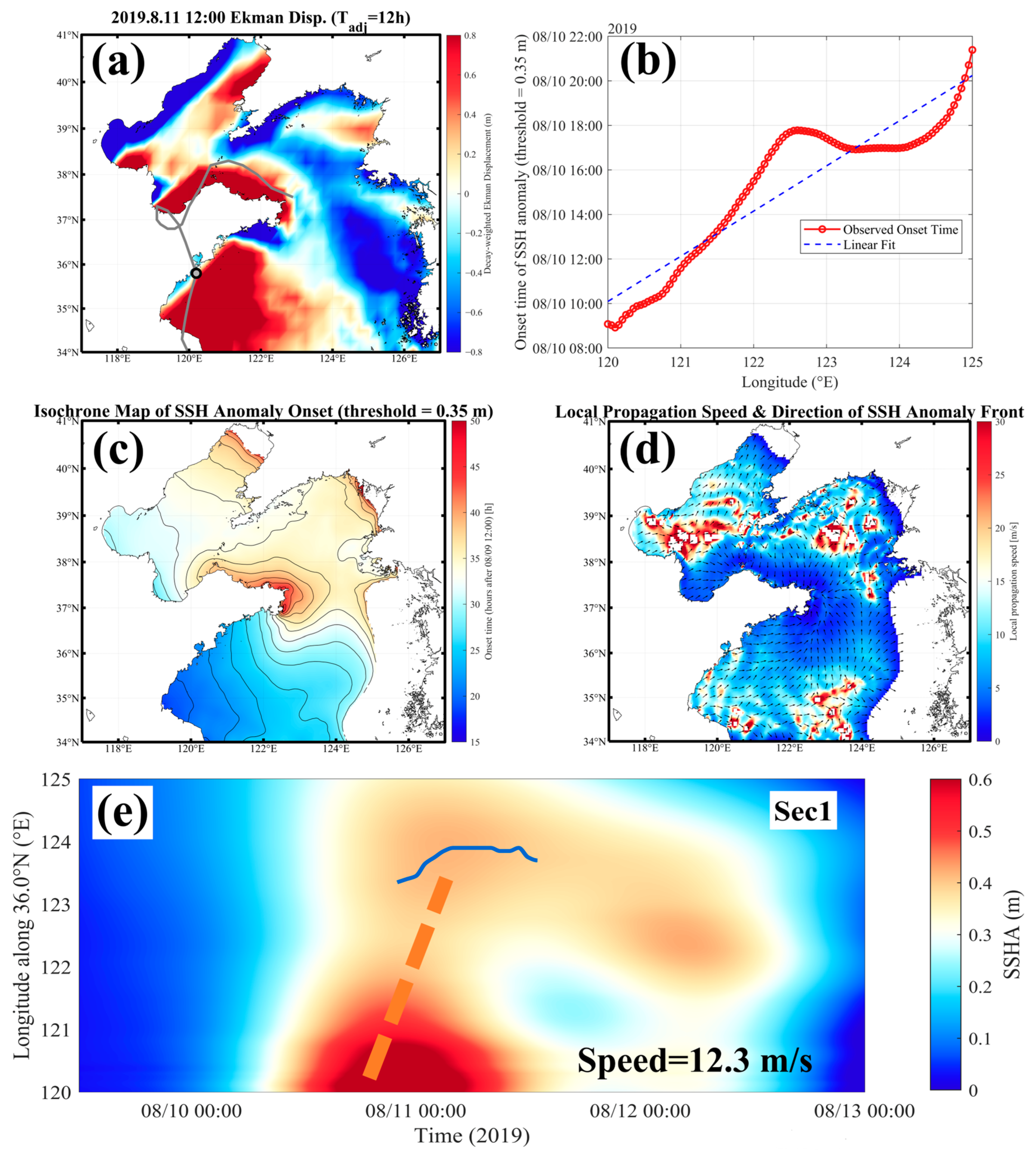
The decay-weighted cumulative Ekman displacement at 12:00 on 11 August (Figure 16a), computed with an adjustment time scale of 12 h consistent with the duration of the anomalous circulation, exhibited a spatially heterogeneous pattern dominated by alternating positive and negative bands aligned with the coast, rather than a coherent sub-basin-scale positive anomaly. This pattern did not correspond to the smooth, sub-basin-scale SSH high documented in Section 3.3.1 (Figure 10), indicating that local wind-driven Ekman transport alone is insufficient to account for the SSHA observed in the basin interior.

Figure 16. Diagnostics of the spatial origin and extension of the SSHA. (a) Decay-weighted cumulative Ekman displacement (color shading) at 12:00 on 11 August 2019, computed with an adjustment time scale of T_adj = 12 h; the grey curve and black-outlined circle denote the typhoon track and instantaneous center position, as in Figure 15. (b) Onset time of the SSHA exceeding a threshold of 0.35 m as a function of longitude along the 36° N transect (Sec1, red circles), together with a linear least-squares fit (blue dashed line). (c) Isochrone map of the SSHA onset time (h, color shading and black contours at 2 h intervals), referenced to 12:00 on 9 August 2019. (d) Local propagation speed (color shading) and direction (black arrows) of the SSHA front, derived from the spatial gradient of the onset-time field shown in (c). (e) Time–distance (Hovmöller) diagrams of SSHA along the zonal transect Sec1 during 9–12 August 2019. The orange dashed line indicates the eastward apparent phase propagation of the leading edge of the positive SSHA, corresponding to 12.3 m s⁻¹. Blue solid lines denote the position of the tracked center of the anomalous anticyclonic circulation at 40 m depth, projected onto each transect. SSHA is referenced to the 7–9 August 2019 mean.

Figure 16. Diagnostics of the spatial origin and extension of the SSHA. (a) Decay-weighted cumulative Ekman displacement (color shading) at 12:00 on 11 August 2019, computed with an adjustment time scale of T_adj = 12 h; the grey curve and black-outlined circle denote the typhoon track and instantaneous center position, as in Figure 15. (b) Onset time of the SSHA exceeding a threshold of 0.35 m as a function of longitude along the 36° N transect (Sec1, red circles), together with a linear least-squares fit (blue dashed line). (c) Isochrone map of the SSHA onset time (h, color shading and black contours at 2 h intervals), referenced to 12:00 on 9 August 2019. (d) Local propagation speed (color shading) and direction (black arrows) of the SSHA front, derived from the spatial gradient of the onset-time field shown in (c). (e) Time–distance (Hovmöller) diagrams of SSHA along the zonal transect Sec1 during 9–12 August 2019. The orange dashed line indicates the eastward apparent phase propagation of the leading edge of the positive SSHA, corresponding to 12.3 m s⁻¹. Blue solid lines denote the position of the tracked center of the anomalous anticyclonic circulation at 40 m depth, projected onto each transect. SSHA is referenced to the 7–9 August 2019 mean.

The onset time of the SSHA along the 36°N transect (Sec1, Figure 16b) generally increased with longitude, consistent with an eastward or basinward extension of the coastal SSH signal. However, the relationship deviated from a simple linear trend, showing a distinct plateau near 122–123° E before resuming its eastward progression. The isochrone map of onset time over the full model domain (Figure 16c) shows that the earliest onset occurred independently along two coastal segments—off the Shandong Peninsula and off northern Jiangsu—with onset time increasing continuously toward the basin interior, where the anomaly threshold was crossed last. This spatial pattern was consistent with the SSH high originating along the coast and subsequently extending into the basin interior, in agreement with the Ekman pumping and cumulative displacement diagnostics described above. A sensitivity analysis (Figure S11) confirms that threshold selection between 0.20–0.40 m yields consistent spatial patterns. For thresholds exceeding 0.40 m, however, the post-decay anomaly signal on 12 August masked the onset-time patterns on 11 August.

To evaluate whether this extension could be quantitatively characterized as wave propagation, the local propagation speed was estimated from the spatial gradient of the onset-time field (Figure 16d). The resulting speed field was spatially heterogeneous, characterized by patchy, small-scale regions of high apparent speed interspersed with near-zero values, particularly within the basin interior, rather than the smooth, slowly varying speed field expected for a single, coherently propagating wavefront. The associated direction field likewise showed locally divergent orientations within the basin rather than a consistent propagation azimuth. This behavior was consistent with the convergence of disturbances originating from multiple, independent coastal source regions with distinct forcing histories, which violated the single coherent wavefront assumption underlying the onset-time gradient method, and precluded a robust, spatially consistent quantitative estimate of propagation speed.

To obtain an independent constraint on the pathway and timescale of the coastal signal, we examined the Hovmöller diagram along Sec1 (Figure 16e). The positive SSHA first intensified at the western end (120.0–121.0° E) between 18:00 on 10 August and 06:00 on 11 August. This location and period coincided precisely with the strongest coastal Ekman convergence and alongshore wind stress off northern Jiangsu, confirming that the western maximum was the wind-driven coastal setup. The elevated SSHA subsequently extended eastward, with the 0.35 m contour advancing from 120.2° E to 123.5° E (~300 km) in approximately 6 h. This advance corresponded to an apparent phase speed of 12.3 m s⁻¹, close to the shallow-water longwave speed of ~14 m s⁻¹ for the ~20 m western shelf and far exceeding the concurrent depth-averaged current speed (<1 m s⁻¹). Water advection was therefore negligible, and the eastward extension was identified as barotropic, free longwave adjustment of the shelf sea-level field. This mechanism rapidly communicated the coastal setup to the basin interior and established the SSH high that drove the subsurface circulation.

4. Discussion

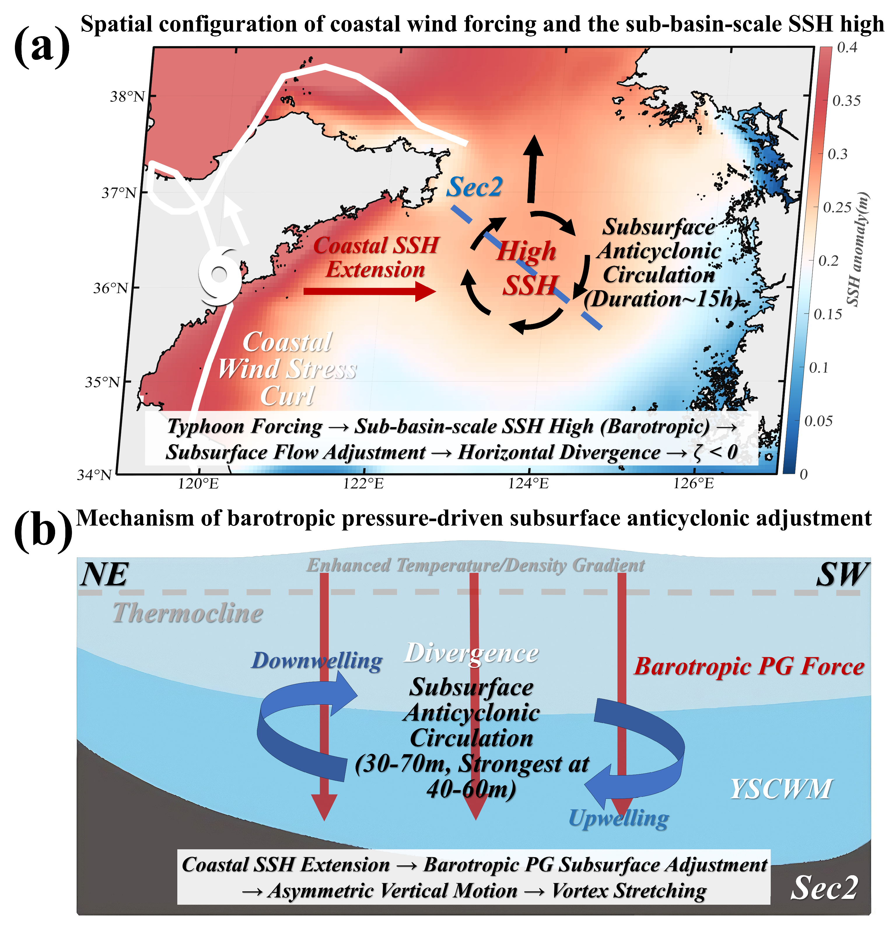
The vorticity budget demonstrates that the vortex stretching term was the primary mechanism responsible for the rapid intensification of anticyclonic (negative) relative vorticity during the typhoon passage. The dominance of the stretching term implies that local horizontal divergence in the subsurface layer was the proximal dynamical cause of the anticyclone formation. This is physically consistent with the response of a stratified water column to a spatially and temporally evolving barotropic pressure field: the nonuniform adjustment of the barotropic pressure anomaly across the water column, modulated by background stratification and bottom topography, can generate horizontal divergence at depth even without direct wind stress penetration to those depths (Figure 17). Vortex stretching as a mechanism for typhoon-induced subsurface vorticity generation has been noted in the context of open-ocean mesoscale eddies [58], but its role in shallow shelf sea environments with strong background stratification and complex bathymetry has received less systematic attention. The present results suggest that the shallow, stratified conditions of the Yellow Sea amplify this process on hourly timescales, producing a rapid and intense anticyclonic response that is shorter in duration than the local inertial period (~17 h). The non-axisymmetric dipole pattern of vertical velocity further indicates that the anticyclone was not a classical isolated eddy driven by central Ekman pumping. Instead, it was an asymmetric three-dimensional adjustment structure. This structure was governed by the combined influence of the barotropic pressure field, background density gradients, spatially nonuniform wind forcing, and bathymetric constraints. The spatial heterogeneity of the horizontal divergence field, as reflected in this dipole pattern, is therefore closely linked to the spatial structure of the anticyclonic vorticity.

Figure 17. Schematic illustrating the spatial origin and dynamical mechanism of the anomalous subsurface anticyclonic circulation induced by Typhoon Lekima. (a) Spatial configuration of coastal wind forcing and the sub-basin-scale SSH high: strong wind stress curl and Ekman pumping along the coastal margins of the Shandong Peninsula and northern Jiangsu generate a sub-basin-scale barotropic SSH high (color shading) in the central South Yellow Sea, which subsequently drives an anticyclonic subsurface circulation at 30–70 m depth (black circular arrows). White arrows indicate the track of Typhoon Lekima. (b) Mechanism of barotropic pressure-driven subsurface anticyclonic adjustment along transect Sec2 (blue dashed line in panel (a)): the depth-independent barotropic pressure gradient force (red arrows) drives an asymmetric adjustment of the water column, producing upwelling on the southwestern side and downwelling on the northeastern side of the anticyclonic circulation, consistent with the dipole vertical velocity pattern documented in Figure 16e. This asymmetric vertical motion generates subsurface horizontal divergence, which promotes vortex stretching and the intensification of anticyclonic (negative) relative vorticity. The enhanced temperature/density gradient near the thermocline (light shading) reflects typhoon-induced weakening of stratification, which facilitated—but did not itself drive—the vertical projection of the barotropic pressure signal into the subsurface.

Figure 17. Schematic illustrating the spatial origin and dynamical mechanism of the anomalous subsurface anticyclonic circulation induced by Typhoon Lekima. (a) Spatial configuration of coastal wind forcing and the sub-basin-scale SSH high: strong wind stress curl and Ekman pumping along the coastal margins of the Shandong Peninsula and northern Jiangsu generate a sub-basin-scale barotropic SSH high (color shading) in the central South Yellow Sea, which subsequently drives an anticyclonic subsurface circulation at 30–70 m depth (black circular arrows). White arrows indicate the track of Typhoon Lekima. (b) Mechanism of barotropic pressure-driven subsurface anticyclonic adjustment along transect Sec2 (blue dashed line in panel (a)): the depth-independent barotropic pressure gradient force (red arrows) drives an asymmetric adjustment of the water column, producing upwelling on the southwestern side and downwelling on the northeastern side of the anticyclonic circulation, consistent with the dipole vertical velocity pattern documented in Figure 16e. This asymmetric vertical motion generates subsurface horizontal divergence, which promotes vortex stretching and the intensification of anticyclonic (negative) relative vorticity. The enhanced temperature/density gradient near the thermocline (light shading) reflects typhoon-induced weakening of stratification, which facilitated—but did not itself drive—the vertical projection of the barotropic pressure signal into the subsurface.

Regarding the potential role of coastal-trapped waves (CTWs), although CTW dynamics are demonstrably active in the Yellow Sea during typhoon forcing, their contribution to the formation of the anomalous circulation can be excluded on temporal grounds. Yan et al. [17], analyzing the same typhoon event, identified significant CTW propagation along the western Yellow Sea only after 18:00 on 11 August—four hours after the anomalous circulation had already dissipated by 14:00 on 11 August. The interior SSHA was thus established and removed well before CTW activity became significant, confirming that CTW dynamics played no role in generating the subsurface circulation analyzed here.

Several limitations of the present study should be acknowledged. First, our analysis is based on a single typhoon event. Whether the subsurface response documented here is representative of other typhoons with different tracks, translation speeds, or intensity profiles remains to be established. Second, we employed the Mellor–Yamada level-2.5 (MY-2.5) turbulence closure to parameterize vertical mixing. Although the core mechanism identified that anticyclonic vorticity generation via vortex stretching is structurally insensitive to the details of vertical mixing, as the barotropic pressure gradient dominates the transient circulation response [59,60], a systematic intercomparison of alternative turbulence closures for this specific event has not been performed. Third, the sensitivity of the identified mechanism to different background stratification conditions, which may vary seasonally and interannually in the Yellow Sea, has not been systematically explored and warrants dedicated future investigation.

5. Conclusions

Based on FVCOM numerical simulations, together with ERA5 reanalysis products and satellite remote sensing data, this study investigated the hourly-scale response of subsurface circulation in the central basin of the South Yellow Sea during the passage of Typhoon Lekima in 2019. The main conclusions are summarized as follows.

(1)

An anomalous middle-scale anticyclonic circulation developed below the thermocline during typhoon passage, identifiable over 30–70 m depth with maximum intensity at 40–60 m. The circulation formed rapidly from the evening of 10 August to early morning of 11 August 2019 and decayed rapidly following typhoon departure, with a total duration of approximately 15 h—shorter than the local inertial period (~17 h). Meanwhile, the radius expanded rapidly at all depths, increasing from approximately 40–80 km to 110–130 km at 40–60 m.

(2)

The core dynamical mechanism is identified as a barotropic pressure-driven rapid adjustment process during the formation and maintenance stages. The anomalous anticyclonic circulation originated from coastal wind forcing along the Shandong Peninsula and northern Jiangsu margins, which generated a barotropic SSHA that rapidly propagated eastward into the central basin of the South Yellow Sea.

Overall, the transient anticyclonic circulation identified below the thermocline during Typhoon Lekima’s passage through the South Yellow Sea resulted from a coastally forced barotropic pressure-driven adjustment mechanism that generated vortex stretching and negative vorticity on hourly timescales. This mechanism represents a previously overlooked class of subsurface dynamical response to extreme typhoon forcing—one that shifts focus from well-documented surface effects (cooling, mixing, coastal processes) to rapid reorganization of subsurface circulation structure. Several directions warrant further investigation. First, although the core mechanism is structurally decoupled from interior mixing parameterizations, a systematic intercomparison of turbulence closures and their interaction with background stratification remains to be conducted to quantify the sensitivity of mixed-layer depth and vertical momentum transfer efficiency to model physics. Second, it remains to be established whether this class of subsurface response is reproducible across a broader range of typhoon track geometries, translation speed and intensity profiles, which would determine its generality beyond the single-event evidence presented here. Finally, the potential consequences of such hourly-scale subsurface reorganizations for the longer-term evolution of the YSCWM, and their sensitivity to the projected poleward migration of tropical cyclone tracks under climate change, require multi-event analysis across varying background stratification conditions. Addressing these questions would advance process-level understanding of how intensifying typhoon activity may alter the three-dimensional circulation and ecosystem functioning of marginal seas.

References

1. Price, J.F. Upper ocean response to a hurricane. J. Phys. Oceanogr. 1981, 11, 153–175. [Google Scholar] [CrossRef] [Scilit]
2. Wentz, F.J.; Gentemann, C.; Smith, D.; Chelton, D. Satellite measurements of sea surface temperature through clouds. Science 2000, 288, 847–850. [Google Scholar] [CrossRef] [Scilit] [PubMed]
3. Chandra, A.; Kumar, S. Sea surface temperature and ocean heat content during tropical cyclones Pam (2015) and Winston (2016) in the Southwest Pacific region. Mon. Weather Rev. 2021, 149, 1173–1187. [Google Scholar] [CrossRef] [Scilit]
4. Jacob, S.D.; Shay, L.K.; Mariano, A.J.; Black, P.G. The 3D oceanic mixed layer response to Hurricane Gilbert. J. Phys. Oceanogr. 2000, 30, 1407–1429. [Google Scholar] [CrossRef] [Scilit]
5. Glenn, S.M.; Miles, T.N.; Seroka, G.N.; Xu, Y.; Forney, R.K.; Yu, F.; Roarty, H.; Schofield, O.; Kohut, J. Stratified coastal ocean interactions with tropical cyclones. Nat. Commun. 2016, 7, 10887. [Google Scholar] [CrossRef] [Scilit] [PubMed]
6. Brooks, D.A. The wake of Hurricane Allen in the western Gulf of Mexico. J. Phys. Oceanogr. 1983, 13, 117–129. [Google Scholar] [CrossRef] [Scilit]
7. Price, J.F. Internal wave wake of a moving storm. Part I: Scales, energy budget and observations. J. Phys. Oceanogr. 1983, 13, 949–965. [Google Scholar] [CrossRef] [Scilit]
8. Gill, A.E. On the behavior of internal waves in the wakes of storms. J. Phys. Oceanogr. 1984, 14, 1129–1151. [Google Scholar] [CrossRef] [Scilit]
9. D’Asaro, E.A. The energy flux from the wind to near-inertial motions in the surface mixed layer. J. Phys. Oceanogr. 1985, 15, 1043–1059. [Google Scholar] [CrossRef] [Scilit]
10. Zedler, S.E.; Dickey, T.D.; Doney, S.C.; Price, J.F.; Yu, X.; Mellor, G.L. Analyses and simulations of the upper ocean’s response to Hurricane Felix at the Bermuda Testbed Mooring site: 13–23 August 1995. J. Geophys. Res. 2002, 107, 25-1–25-29. [Google Scholar] [CrossRef] [Scilit]
11. Sanford, T.B.; Price, J.F.; Girton, J.B. Upper-ocean response to Hurricane Frances (2004) observed by profiling EM-APEX floats. J. Phys. Oceanogr. 2011, 41, 1041–1056. [Google Scholar] [CrossRef] [Scilit]
12. Hsu, P.C.; Ho, C.R. Typhoon-induced ocean subsurface variations from glider data in the Kuroshio region adjacent to Taiwan. J. Oceanogr. 2018, 75, 1–21. [Google Scholar] [CrossRef] [Scilit]
13. Zhang, H.; Xie, X.H.; Yang, C.H.; Qi, Y.F.; Tian, D.; Xu, J.X.; Cai, S.Q.; Wu, R.H.; Ma, Y.L.; Ni, X.B.; et al. Observed impact of Typhoon Mangkhut (2018) on a continental slope in the South China Sea. J. Geophys. Res. Oceans 2022, 127, e2022JC018432. [Google Scholar] [CrossRef] [Scilit]
14. Liu, X.C.; Gu, Y.Z.; Zhai, F.G.; Li, P.L.; Liu, Z.Z.; Bai, P.; Liu, C.; Sun, L.Y.; Wu, K.J. Dramatic temperature variations in the Yellow Sea during the passage of typhoon Lekima (2019). Estuar. Coast. Shelf Sci. 2022, 269, 107819. [Google Scholar] [CrossRef] [Scilit]
15. Liu, X.C.; Zhai, F.G.; Yan, J.J.; Gu, Y.Z.; Wang, Y.C.; Li, P.L.; Wu, K.J. Three-dimensional temperature responses to northward-moving typhoons in the shallow stratified Yellow Sea in summer. J. Geophys. Res. Oceans 2022, 127, e2022JC019091. [Google Scholar] [CrossRef] [Scilit]
16. Lu, Q.Y.; Liu, Y.H.; Guan, S.D. Differences in the response of the deep ocean in the Northwest Pacific and the coastal seas of China to Super Typhoon Chantu (2021). Oceanol. Limnol. Sin. 2025, 56, 792–805. [Google Scholar]
17. Yan, J.J.; Zhai, F.G.; Gu, Y.Z.; Liu, X.C.; Li, P.L.; Liu, Z.Z.; Wang, Y.C. Drastic fluctuation in water exchange between the Yellow Sea and Bohai Sea caused by Typhoon Lekima in August 2019: A numerical study. J. Geophys. Res. Oceans 2023, 128, e2022JC019260. [Google Scholar] [CrossRef] [Scilit]
18. Moon, I.J.; Kwon, S.J. Impact of upper-ocean thermal structure on the intensity of Korean peninsular landfall typhoons. Prog. Oceanogr. 2012, 105, 61–66. [Google Scholar] [CrossRef] [Scilit]
19. Guan, S.D.; Li, S.Q.; Hou, Y.J.; Hu, P.; Liu, Z.; Feng, J.Q. Increasing threat of landfalling typhoons in the western North Pacific between 1974 and 2013. Int. J. Appl. Earth Obs. Geoinf. 2018, 68, 279–286. [Google Scholar] [CrossRef] [Scilit]
20. Chan, J.C.L.; Shi, J.E. Long-term trends and interannual variability in tropical cyclone activity over the western North Pacific. Geophys. Res. Lett. 1996, 23, 2765–2767. [Google Scholar] [CrossRef] [Scilit]
21. He, C.B.; Wang, Y.X.; Lei, Z.Y.; Xu, S. A preliminary study on the formation and properties of the Yellow Sea Cold Water Mass. Oceanol. Limnol. Sin. 1959, 2, 11–15. [Google Scholar]
22. Zhang, S.W.; Wang, Q.Y.; Lü, Y.; Cui, H.; Yuan, Y.L. Observation of the seasonal evolution of the Yellow Sea Cold Water Mass in 1996–1998. Cont. Shelf Res. 2008, 28, 442–457. [Google Scholar] [CrossRef] [Scilit]
23. Li, A. Study on the Interannual Variation of the Yellow Sea Cold Water Mass. Ph.D. Thesis, University of Chinese Academy of Sciences, Beijing, China, 2016. [Google Scholar]
24. Zhang, S.W.; Xia, C.S.; Yuan, Y.L. The physical-ecological coupling numerical models in the Yellow Sea Cold Water Mass. Prog. Nat. Sci. 2002, 12, 315–319. [Google Scholar]
25. Zhang, G.T.; Sun, S.; Yang, B. Summer reproduction of the planktonic copepod Calanus sinicus in the Yellow Sea: Influences of high surface temperature and cold bottom water. J. Plankton Res. 2007, 29, 179–186. [Google Scholar] [CrossRef] [Scilit]
26. Wang, B.; Hirose, N.; Kang, B.; Takayama, K. Seasonal migration of the Yellow Sea Bottom Cold Water. J. Geophys. Res. Oceans 2014, 119, 4430–4443. [Google Scholar] [CrossRef] [Scilit]
27. Hu, Y.B. Characteristics and Mechanisms of the Circulation and Near-Inertial Oscillations of the Yellow Sea Cold Water Mass. Ph.D. Thesis, University of Chinese Academy of Sciences, Beijing, China, 2024. [Google Scholar]
28. Lee, J.H.; Pang, I.C.; Moon, J.H. Contribution of the Yellow Sea bottom cold water to the abnormal cooling of sea surface temperature in the summer of 2011. J. Geophys. Res. Oceans 2016, 121, 7052–7068. [Google Scholar] [CrossRef] [Scilit]
29. Yang, G.B.; Lü, L.G.; Zhuang, Z.P.; Xiong, X.J.; Wang, G.S.; Guo, Y.L.; Yu, L.; Ma, D.J. Cruise observation of shallow water response to typhoon Damrey 2012 in the Yellow Sea. Cont. Shelf Res. 2017, 148, 1–8. [Google Scholar] [CrossRef] [Scilit]
30. Yu, H.; Wang, N.; Ding, Y.; Li, R.; Bao, X.; Gao, G.; Bi, C.; Zhou, L.; Yao, Z.; Wan, K. Observed and model-simulated dramatic bottom temperature variations during a weakened typhoon in the northern Yellow Sea. J. Geophys. Res. Oceans 2025, 130, e2025JC022401. [Google Scholar] [CrossRef] [Scilit]
31. Kim, C.S.; Lim, H.S.; Jeong, J.Y.; Shim, J.S.; Moon, I.J.; Oh, Y.J.; You, H.Y. Responses of coastal waters in the Yellow Sea to Typhoon Bolaven. J. Coast. Res. 2014, 70, 278–283. [Google Scholar] [CrossRef] [Scilit]
32. Yu, B.; Ge, Y.; Ren, D.J.; Ji, C.Z.; Hu, W. Observational study of the Yellow Sea response to Typhoon Lekima. Mar. Sci. 2022, 46, 34–43. [Google Scholar] [CrossRef]
33. Ji, C.Z.; Ge, Y.; Li, J.; Yu, B.; Liu, Q. Observational study of the Yellow Sea ocean response to the peripheral process of Typhoon Chan-hom. Acta Oceanol. Sin. 2020, 42, 46–53. [Google Scholar]
34. Wang, X.W.; Wang, X.J.; You, Z.J. Variations of chlorophyll-a and particulate organic carbon in the Yellow-Bohai Sea: In response to the Typhoon Lekima event. Geosci. Lett. 2021, 8, 30. [Google Scholar] [CrossRef] [Scilit]
35. Chai, X. Study on the Anomalous Sea Surface Temperature Warming Event in the Yellow Sea During the Passage of Typhoon Bolaven (2012). Master’s Thesis, Nanjing University of Information Science and Technology, Nanjing, China, 2019. [Google Scholar]
36. Li, Y.; Wang, A.J.; Qiao, L.; Fang, J.; Chen, J. The impact of typhoon Morakot on the modern sedimentary environment of the mud deposition center off the Zhejiang-Fujian coast, China. Cont. Shelf Res. 2012, 37, 92–100. [Google Scholar] [CrossRef] [Scilit]
37. Ma, Y.P.; Zhai, F.G.; Liu, X.C.; Liu, C.; Liu, Z.Z.; Gu, Y.Z.; Li, P.L. Three-dimensional changes in temperature and circulation caused by northwestward-moving typhoons in a temperate semi-enclosed shelf sea in summer. Front. Mar. Sci. 2025, 12, 1512102. [Google Scholar] [CrossRef] [Scilit]
38. Martell-Dubois, R.; Silva-Casarín, R.; Mendoza-Baldwin, E.G.; Muñoz-Pérez, J.J.; Cerdeira-Estrada, S.; Escalante-Mancera, E.; Laiz, I. Spectral bimodality of waves produced by hurricanes in the Caribbean coastal zone off Mexico. Cienc. Mar. 2018, 44, 33–48. [Google Scholar] [CrossRef] [Scilit]
39. Chen, C.S.; Liu, H.D.; Beardsley, R.C. An unstructured grid, finite-volume, three-dimensional, primitive equations ocean model: Application to coastal ocean and estuaries. J. Atmos. Ocean. Technol. 2003, 20, 159–186. [Google Scholar] [CrossRef] [Scilit]
40. Chen, C.S.; Beardsley, R.C.; Cowles, G. An unstructured grid, finite-volume coastal ocean model (FVCOM) system. Oceanography 2006, 19, 78–89. [Google Scholar] [CrossRef] [Scilit]
41. Hersbach, H.; Bell, B.; Berrisford, P.; Hirahara, S.; Horányi, A.; Muñoz-Sabater, J.; Nicolas, J.; Peubey, C.; Radu, R.; Schepers, D.; et al. The ERA5 global reanalysis. Q. J. R. Meteorol. Soc. 2020, 146, 1999–2049. [Google Scholar] [CrossRef] [Scilit]
42. Jean-Michel, L.; Eric, G.; Romain, B.-B.; Gilles, G.; Angélique, M.; Marie, D.; Clément, B.; Mathieu, H.; Olivier, L.G.; Charly, R.; et al. The Copernicus Global 1/12° Oceanic and Sea Ice GLORYS12 Reanalysis. Front. Earth Sci. 2021, 9, 698876. [Google Scholar] [CrossRef] [Scilit]
43. Egbert, G.D.; Erofeeva, S.Y. Efficient inverse modeling of barotropic ocean tides. J. Atmos. Ocean. Technol. 2002, 19, 183–204. [Google Scholar] [CrossRef] [Scilit]
44. Chen, C.; Beardsley, R.C.; Cowles, G.; Qi, J.; Lai, Z.; Gao, G.; Lin, H. FVCOM User Manual, 3rd ed.; University of Massachusetts Dartmouth: Dartmouth, MA, USA, 2011. [Google Scholar]
45. Ding, Y.; Bao, X.W.; Yao, Z.G.; Song, D.H.; Song, J.; Gao, J.; Li, J. Effect of coastal-trapped waves on the synoptic variations of the Yellow Sea Warm Current during winter. Cont. Shelf Res. 2018, 167, 14–31. [Google Scholar] [CrossRef] [Scilit]
46. Ding, Y.; Bao, X.W.; Yao, Z.G.; Bi, C.C.; Wan, K.; Bao, M.; Jiang, Z.P.; Song, J.; Gao, J. Observational and model studies of synoptic current fluctuations in the Bohai Strait on the Chinese continental shelf. Ocean Dyn. 2019, 69, 323–351. [Google Scholar] [CrossRef] [Scilit]
47. Ding, Y.; Bao, X.W.; Zhou, L.; Bi, C.C.; Yao, Z.G.; Ma, C.; Chu, Q.Q. Modeling the westward transversal current in the southern Yellow Sea entrance: A case study in winter 2007. Ocean Dyn. 2020, 70, 803–825. [Google Scholar] [CrossRef] [Scilit]
48. Gao, G.D.; Wang, X.H.; Song, D.H.; Bao, X.W.; Yin, B.S.; Ding, Y.; Li, H.; Hou, F.; Ren, Z. Effects of wave–current interactions on suspended-sediment dynamics during strong wave events in Jiaozhou Bay, Qingdao, China. J. Phys. Oceanogr. 2018, 48, 1053–1078. [Google Scholar] [CrossRef] [Scilit]
49. Lee, J.H.; Moon, J.H.; Kim, T. Typhoon-triggered phytoplankton bloom and associated upper-ocean conditions in the Northwestern Pacific: Evidence from satellite remote sensing, Argo profile, and an ocean circulation model. J. Mar. Sci. Eng. 2020, 8, 788. [Google Scholar] [CrossRef] [Scilit]
50. Yang, Y.; Li, K.P.; Du, J.T.; Liu, Y.L.; Liu, L.; Wang, H.W.; Yu, W.D. Revealing the subsurface Yellow Sea Cold Water Mass from satellite data associated with Typhoon Muifa. J. Geophys. Res. Oceans 2019, 124, 7135–7152. [Google Scholar] [CrossRef] [Scilit]
51. Li, C.; Hou, Y.; Li, S.; Li, J. Characteristics of wave field in the Yellow Sea and the Bohai Sea under the influence of two typical typhoons. Oceanol. Limnol. Sin. 2021, 52, 51–65, (In Chinese with English abstract). [Google Scholar] [CrossRef]
52. Nencioli, F.; Dong, C.; Dickey, T.; Washburn, L.; McWilliams, J.C. A vector geometry-based eddy detection algorithm and its application to a high-resolution numerical model product and high-frequency radar surface velocities in the Southern California Bight. J. Atmos. Ocean. Technol. 2010, 27, 564–579. [Google Scholar] [CrossRef] [Scilit]
53. Pedlosky, J. Geophysical Fluid Dynamics, 2nd ed.; Springer: New York, NY, USA, 1987; 710p. [Google Scholar]
54. Cushman-Roisin, B.; Beckers, J.M. Introduction to Geophysical Fluid Dynamics: Physical and Numerical Aspects, 2nd ed.; Academic Press: Cambridge, MA, USA, 2011; 828p. [Google Scholar]
55. Zhao, C.; Wang, N.; Ding, Y.; Song, D.; Li, J.; Li, M.; Zhou, L.; Yu, H.; Chen, Y.; Bao, X. Numerical Study on the Formation Mechanism of Plume Bulge in the Pearl River Estuary under the Influence of River Discharge. Water 2024, 16, 1296. [Google Scholar] [CrossRef] [Scilit]
56. Alessi, C.A.; Beardsley, R.C.; Limeburner, R.; Rosenfeld, L.K.; Lentz, S.J.; Send, E.; Winant, C.D.; Allen, J.S.; Halliwell, G.R., Jr.; Brown, W.S.; et al. CODE-2: Moored Array and Large-Scale Data Report; Limeburner, R., Ed.; Technical Report WHOI-85-35; CODE Technical Report No. 38; Woods Hole Oceanographic Institution: Woods Hole, MA, USA, 1985. [Google Scholar] [CrossRef] [Scilit]
57. Zhang, Z.; Ma, Z.; Fei, J.; Zheng, Y.; Huang, J. The effects of tropical cyclones on characteristics of barrier layer thickness. Front. Earth Sci. 2022, 10, 962232. [Google Scholar] [CrossRef] [Scilit]
58. Jaimes, B.; Shay, L.K. Mixed layer cooling in mesoscale oceanic eddies during Hurricanes Katrina and Rita. Mon. Weather Rev. 2009, 137, 4188–4207. [Google Scholar] [CrossRef] [Scilit]
59. Price, J.F.; Sanford, T.B.; Forristall, G.Z. Forced stage response to a moving hurricane. J. Phys. Oceanogr. 1994, 24, 233–260. [Google Scholar] [CrossRef] [Scilit]
60. Kudryavtsev, V.; Monzikova, A.; Combot, C.; Chapron, B.; Reul, N. A simplified model for the baroclinic and barotropic ocean response to moving tropical cyclones: 2. Model and simulations. J. Geophys. Res. Oceans 2019, 124, 3462–3485. [Google Scholar] [CrossRef] [Scilit]
61. Chen, C.; Huang, H.; Beardsley, R.C.; Liu, H.; Xu, Q.; Cowles, G. A finite-volume numerical approach for coastal ocean circulation studies: Comparisons with finite-difference models. J. Geophys. Res. 2007, 112, C03018. [Google Scholar] [CrossRef] [Scilit]
Figure 1. Regional map and topography of the Bohai Sea (BS) and Yellow Sea (YS), and the path of Typhoon Lekima. The magenta line, yellow pentagram, and colored dots respectively denote the track of Typhoon Lekima during August 2019, its center positions at 0000 UTC on 10, 11, and 12 August, and the maximum wind speed at 6 h intervals. Color shading represents bathymetric depths in meters. White-dashed line delineates the boundary of the Yellow Sea Cold Water Mass (YSCWM), defined by the 11 °C isotherm of the model-simulated monthly mean temperature at a depth of 40 m for August 2019. Purple-dashed rectangle indicates the central South Yellow Sea region of interest. The white solid line denotes the zonal transect (Section 1), used to assess the vertical structure of temperature and density, as discussed in Section 3. Red arrows indicate the Yangtze River, the Yellow River, and the Yalu River, respectively. The green dot with a white outer ring denotes the bottom-temperature observation station (T1), while the blue dots with white outer rings denote the three sea-level observation stations (G1–G3).
Jmse 14 01691 g001
Figure 2. Validation of the FVCOM simulation against hourly in situ observations. (a) Bottom-layer temperature (BLT) at mooring T1 in the central South Yellow Sea from 8 to 21 August 2019; black, observation; red, simulation. (bd) Residual (detided, 36 h low-passed) sea level (m) at tide-gauge stations G1 (b), G2 (c) and G3 (d) from 2 to 29 August 2019. Temporal correlation coefficients (TCC) and root mean square errors (RMSE) are given in each panel; all correlations are significant at the 99% level after accounting for serial correlation through the effective number of degrees of freedom. Station locations are given in Figure 1. Note the different time axis in (a), which is limited by the availability of the mooring record.
Jmse 14 01691 g002
Figure 3. Track comparison and synoptic-scale 10 m wind field evolution of Typhoon Lekima (2019) over the East China Sea and adjacent landmasses. (a) Observed best track from IBTrACS (black solid line with circles) versus ERA5 reanalysis-based vortex tracking (red dashed line with crosses). Gray dotted lines connect corresponding 6-hourly positions; date labels (MM/DD) are shown at 12 h intervals. (bf) Fourier-filtered 10 m wind speed (shading; m s−1) and wind barbs (full barb = 5 m s−1) at selected synoptic times: 1800 UTC 10 August, 0000 UTC 11 August, 0600 UTC 11 August, 1200 UTC 11 August, and 1800 UTC 11 August 2019. Red polygons denote the 34 kt (≈63 km h−1) wind radii (R34) in each quadrant (NE, SE, SW, NW) derived from IBTrACS advisory data, with radial extents annotated in kilometers. Red stars and open black circles indicate the ERA5-derived and IBTrACS-reported tropical cyclone centers, respectively. The color bar applies to panels (bf).
Jmse 14 01691 g003
Figure 4. Comparison of sea surface temperature (SST) between REMSS satellite observations (ai) and FVCOM simulations (jr) over the Bohai–Yellow Sea region from 7 to 15 August 2019, with one panel per day. Isotherms are omitted for clarity. (s) Spatial distribution of the temporal correlation coefficient (TCC) between daily simulated and observed SST from 7 to 15 August 2019; semi-transparent black dots indicate grid points where TCC is statistically significant (p < 0.05). (t) Spatial distribution of the temporal root mean square error (RMSE) between simulations and observations. (u) Time series of the domain-averaged spatial correlation coefficient (SCC; left axis, blue line) and RMSE (right axis, red line) computed daily over the Yellow Sea from 7 to 15 August 2019.
Jmse 14 01691 g004
Figure 5. Comparison of sea surface height (SSH) between CMEMS satellite altimetry observations (ai) and FVCOM simulations (jr) over the Bohai–Yellow Sea region from 7 to 15 August 2019, with one panel per day. (s) Spatial distribution of the TCC between daily simulated and observed SSH from 7 to 15 August 2019; semi-transparent black dots indicate grid points where TCC is statistically significant (p < 0.05). (t) Spatial distribution of the temporal RMSE between simulations and observations. (u) Time series of the domain-averaged SCC (left axis, blue line) and RMSE (right axis, red line) computed daily over the central South Yellow Sea from 7 to 15 August 2019.
Jmse 14 01691 g005
Figure 7. (at) Bottom current fields in the Yellow Sea from 10 to 12 August 2019, same as Figure 6. The current velocity data have been subjected to a 36 h low-pass filter.
Jmse 14 01691 g007
Figure 8. Relative vorticity at 30 m depth in the Yellow Sea (a) before, (b) during, and (c) after typhoon passage. Negative values (blue shading) indicate anticyclonic rotation, and positive values (red shading) indicate cyclonic rotation. Black arrows show the current vectors at 30 m depth. The grey curve indicates the track of Typhoon Lekima, and the dot with a black outline and grey center marks the typhoon center position at the corresponding time. The current velocity data have been subjected to a 36 h low-pass filter.
Jmse 14 01691 g008
Figure 9. (a) Temporal evolution of the center positions of the anomalous anticyclonic circulation at depths of 30, 40, 50, 60, and 70 m from 21:00 on 10 August to 13:00 on 11 August 2019 (UTC). The center positions at 30, 40, 50, 60, and 70 m are shown in green, blue, red, orange, and purple, respectively, plotted at hourly intervals, with squares marking the starting points, circles the intermediate points, and triangles the end points. The grey dashed line at 0 m denotes the projected trajectory of the circulation centers across all depth levels. (b) Temporal evolution of the estimated radius of the anomalous anticyclonic circulation at depths of 30, 40, 50, 60, and 70 m over the same period. Line colors correspond to the different depths as in Figure 9a and are indicated in the legend.
Jmse 14 01691 g009
Figure 10. (at) SSH (color shading) and 30 m currents (black arrows) in the Yellow Sea from 10 to 12 August 2019, at the same time steps as Figure 6. The grey curve indicates the track of Typhoon Lekima, and the dot with a black outline and grey center marks the typhoon center position at the corresponding time. The current velocity data have been subjected to a 36 h low-pass filter.
Jmse 14 01691 g010
Figure 11. Temporal evolution of the momentum budget terms for the anomalous anticyclonic circulation, area-averaged over the circulation region, at depths of (a,f) 30 m, (b,g) 40 m, (c,h) 50 m, (d,i) 60 m, and (e,j) 70 m, from 22:00 on 10 August to 14:00 on 11 August 2019 (UTC). Panels (ae) show the zonal (eastward) momentum budget; panels (fj) show the meridional (northward) momentum budget. Terms shown include local acceleration (ACCEL, black), nonlinear horizontal advection (ADV, red), the Coriolis force (COR, blue), vertical turbulent viscosity (VVISC, orange), the baroclinic component of the pressure gradient force (PGBC, purple), and the barotropic component of the pressure gradient force (PGBT, green).
Jmse 14 01691 g011
Figure 12. (at) Vertical sections of temperature gradient (color shading) and potential density isopycnals (kg m−3, black contours) along Sec1 (36° N) in the South Yellow Sea from 10 to 12 August 2019, at the same time steps as Figure 6. The horizontal axis denotes longitude (°E) and the vertical axis denotes depth (m). Warm colors indicate large temperature gradients associated with the thermocline.
Jmse 14 01691 g012
Figure 13. Temporal evolution of the vorticity budget terms for the anomalous anticyclonic circulation, area-averaged over the circulation region, at depths of (a) 30 m, (b) 40 m, (c) 50 m, (d) 60 m, and (e) 70 m, from 22:00 on 10 August to 14:00 on 11 August 2019 (UTC). Terms shown include the local rate of change of relative vorticity (LCT, black), the advection term (VA, red), planetary vorticity, or the β-effect (LV, blue), the vortex stretching term (DT, yellow), the tilting term (TT, purple), the baroclinic term (BT, green), and the frictional term (FT, orange). Positive values indicate cyclonic vorticity tendency; negative values indicate anticyclonic vorticity tendency.
Jmse 14 01691 g013
Figure 14. (at) Vortex stretching tendency (color shading) at 30 m depth in the Yellow Sea from 10 to 12 August 2019, at the same time steps as Figure 6. Negative values (blue) indicate a tendency to generate anticyclonic (negative) relative vorticity; positive values (red) indicate a cyclonic tendency.
Jmse 14 01691 g014