High-Dimensional Clustering-Driven Performance Evaluation and Mutation-Centric Early Warning for Marine Diesel Engines

Abstract

To proactively identify performance anomaly evolution and potential operational risks of marine main engines and reserve a sufficient time window for maintenance intervention, this paper proposes a data-driven multi-algorithm fusion framework for performance evaluation and anomaly early warning of marine main engines. The framework first adopts a steady-state detection strategy to filter valid operating conditions and introduces the CLIQUE clustering algorithm to realize adaptive partitioning of high-dimensional operating parameters; comparative experiments with the classical K-means++ clustering algorithm demonstrate that CLIQUE achieves finer-grained operating condition classification without pre-defining the number of clusters and better adapts to the uneven distribution of actual marine engine operating conditions, which addresses the limitations of traditional single-parameter analysis and conventional dimensionality reduction methods in practical shipboard scenarios. On this basis, the Mahalanobis distance evaluation model is constructed under each partitioned operating condition, which further improves the stability and anti-interference performance of quantitative performance assessment for the main engine. Meanwhile, by integrating cumulative anomaly trend analysis and the Yamamoto mutation test, the framework accurately captures statistical mutation characteristics of the performance deviation trajectory and identifies the first mutation point as the retrospective candidate change point, forming a systematic anomaly detection mechanism. Validation using field measurement data from a 6RT-flex82T marine main engine shows that the proposed framework can comprehensively characterize the overall operating state of the main engine and capture long-term performance deviation evolution patterns. Retrospective analysis indicates that the first statistical mutation of the multivariate performance deviation precedes the significant abnormal fluctuation of a single parameter by approximately 20 days, showing the potential of providing a maintenance buffer period. The proposed method can provide technical reference and support for condition-based maintenance of marine main engines and intelligent operation and maintenance of shipboard power equipment.

1. Introduction

The main engine is the core power plant of a ship, which operates under high loads over extended periods in harsh marine environments. Owing to the combined effects of operating conditions and environmental factors, incipient anomalies and performance deviations may occur continuously. Accurate performance evaluation and anomaly early warning for the main engine can reserve sufficient time windows for preventive maintenance and proactive condition-based intervention, which are of critical importance for ensuring navigation safety and improving operational economy. However, the marine main engine system is structurally complex and subject to varying operating conditions. Traditional monitoring approaches often collect only a limited number of parameters, making it difficult to fully characterize the true performance state of the equipment. Meanwhile, the incipient degradation features of the main engine are easily masked by strong operational fluctuations and background monitoring noise, which poses practical challenges for conventional fixed-threshold warning methods, including limited sensitivity and relatively high false-alarm risks. With the introduction of the smart ship concept and its industrial advancement, prognostics and health management (PHM) technology has become a core technical pathway for enabling intelligent operation and maintenance of marine power equipment [1,2,3,4,5,6,7]. Among these, data-driven PHM methods can be further divided into pure data-driven paradigms and physics-informed fusion frameworks [8]. Pure data-driven approaches do not rely on precise and complex physical mechanism models; instead, they construct state assessment and prediction models merely by mining the implicit patterns in historical and real-time monitoring data. The effectiveness of such methods has been validated in numerous engineering practices [5,6,7]. The current consensus in this research field indicates that integrating multi-source monitoring data, intelligent algorithms, and state perception technologies for health assessment and intelligent anomaly detection of marine power equipment has become an inevitable trend in the industry [6,7].

A reliable performance evaluation of the main engine must be based on steady-state operating data [9]. Among various steady-state detection algorithms, the SSD algorithm, owing to its simple parameter settings and its capability to perform collaborative statistical tests on multiple parameters, demonstrates robust performance and practicality in steady-state identification for complex systems [10]; therefore, it is adopted in this study to screen effective data intervals for analysis. Current anomaly early warning research for power equipment can be broadly classified into two core approaches: state prediction-based and state classification-based methods. Among them, state prediction methods (e.g., CNN-BiGRU, PCA-CNN-BiLSTM models) may face limited generalization in practical shipboard scenarios due to scarce labeled fault samples when dealing with complex abnormal conditions and high-dimensional, time-varying parameters [11,12,13]. In contrast, data-driven state classification methods combined with time series statistical analysis can more objectively extract statistical features of state evolution from multidimensional monitoring data [14,15]. Clustering analysis (e.g., K-means++, EM algorithm) and time series analysis are common technical tools in this category [16,17,18,19,20,21]. However, most existing studies employ only a single or a few reduced-dimension features to characterize the overall engine performance, which is prone to the loss of critical information and leads to a one-sided performance evaluation [19,22].

To address the limitations of the existing studies mentioned above, this paper proposes an integrated analytical framework combining multiple mature algorithms. First, multiple long-term operating parameters covering several subsystems of the main engine are collected, and then, the SSD algorithm is used to filter out interfering data from non-steady-state conditions. Next, the CLIQUE clustering algorithm is innovatively introduced to autonomously partition the high-dimensional steady-state operating conditions. This method can effectively handle the complex coupling relationships among multiple parameters, achieving more objective and refined condition classification than traditional single-parameter analysis and conventional dimensionality reduction approaches [13,16,19]. After condition partitioning, the Mahalanobis distance under each condition is further computed to quantify the temporal evolution of the overall engine performance. Finally, time-domain mutation detection techniques are applied to analyze the performance deviation curve, precisely locating statistical tipping points of performance deviation, thereby enabling more timely and accurate retrospective identification. The validation results based on real-ship operational cases fully demonstrate the effectiveness and engineering application potential of the proposed method.

2. Performance Evaluation Indicators

2.1. Data Source

The monitoring data used in this study are derived from a Wärtsilä 6RT-flex82T (Wärtsilä Corporation, Helsinki, Finland) main engine installed on board a certain vessel. Prior to June 2020, the vessel completed scheduled docking repair, where a dedicated data-acquisition system for engine-room equipment condition monitoring was retrofitted. After the repair and system commissioning, the vessel resumed regular sea-going operations. Consequently, the initial segment of the dataset corresponds to the engine’s operational status right after overhaul, which provides the basis for selecting the health-reference baseline in subsequent analysis. The dataset comprises 43,186 performance monitoring samples, spanning from 6:20 on 9 June 2020 to 8:10 on 14 May 2021. The main technical parameters of the engine are listed in

Table 1. Technical specifications of the 6RT-flex82T marine main engine.

Technical Parameter	Value
Number of cylinders	6
Bore diameter/mm	820
Stroke/mm	3375
Firing order	1-5-3-4-2-6
Rated power/kW	25,200
Rated speed/(r/min)	76
Rated specific fuel consumption/(g/kW·h)	176.7
Operating power/kW	22,680
Operating speed/(r/min)	72
Operating fuel consumption/(g/kW·h)	200.02
Critical speed/(r/min)	34–45
Number of turbochargers	2
Engine type	Vertical two-stroke engine

.

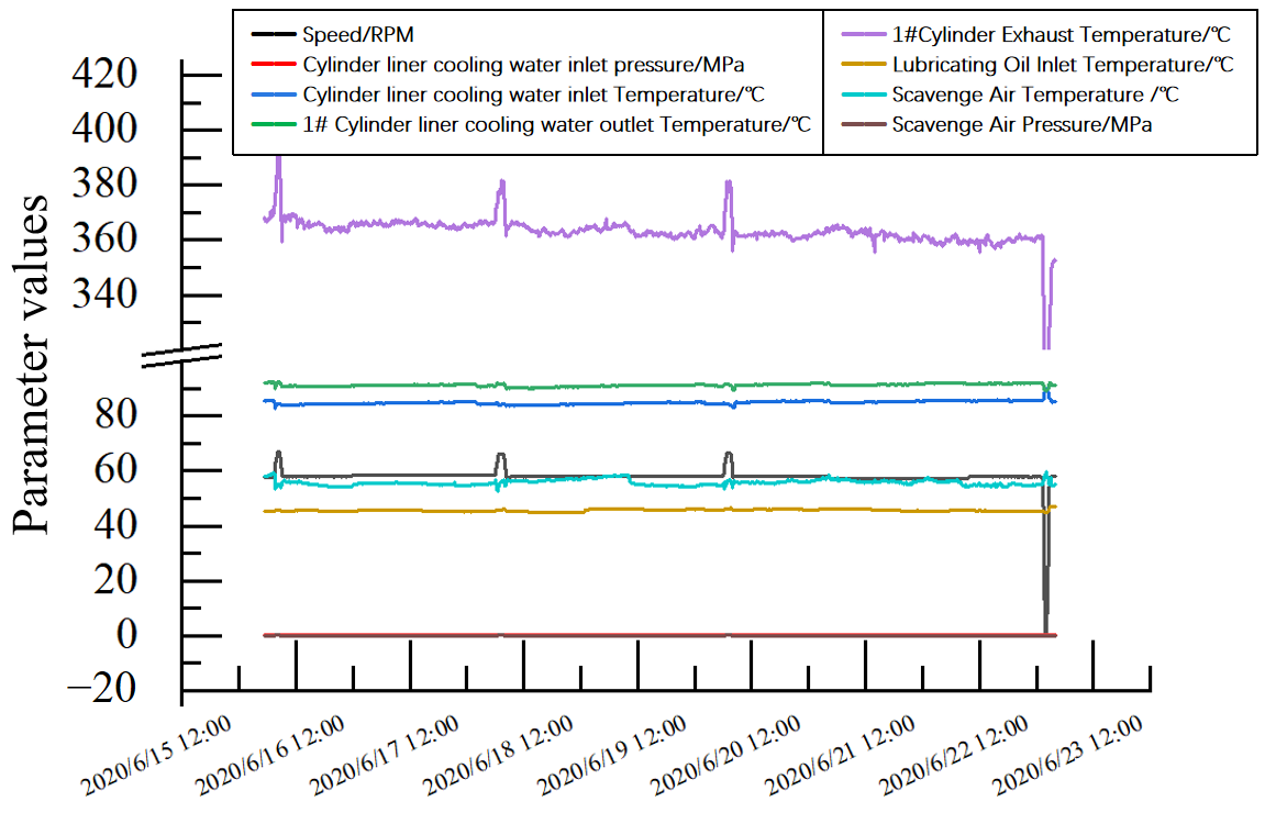
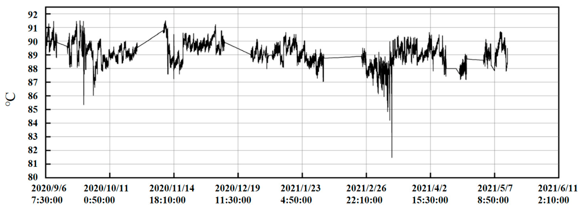
The monitoring parameters in this paper are collected and stored by the data-acquisition system mentioned above. The system supports four hierarchical sampling-storage modes: the raw high-frequency dataset is obtained at a 1 s sampling interval, which is further down-sampled to produce derived datasets at 1 min, 10 min and 1 h intervals. Each record consists of sampling time, data type, parameter value and parameter category. Under steady-sea navigation, main engine condition transitions are rare, and stable operation may last several to tens of hours. The 10 min granularity can capture representative operating features and suppress short-term random measurement noise for long-term deviation evaluation while providing moderately sized samples to guarantee statistical reliability for condition clustering and mutation detection with restrained computational overhead. Accordingly, the 10 min dataset is selected as the unified time step for analysis. As shown in Figure 1, numerous abnormal data points are observed within the 10 min subset from 05:30 on 16 June 2020 to 04:00 on 23 June 2020. Preprocessing is therefore required prior to data usage, and relevant approaches are described in Section 3.

2.2. Determination of Performance Parameters

The conventional thermal parameters of a marine main engine can effectively reflect its operational health status. At present, most of these conventional thermal parameters are automatically monitored, collected, and stored in real-time [13]. Performance-related deviations of marine engines are largely exhibited as departures of conventional thermal parameters from factory-calibrated baselines. Thus, such deviation metrics can be adopted as performance-evaluation indicators to quantify the magnitude of performance drift.

Rational selection of performance parameters lays the foundation for engine performance evaluation. In this paper, 22 parameters are adopted for the overall performance assessment of the marine main engine, including power, fuel type, rotational speed, scavenging air temperature, fuel flow rate, specific fuel oil consumption, exhaust gas temperatures of cylinders #1–#6, cooling water outlet temperatures of cylinder liners #1–#6, lubricating oil inlet temperature, cooling water inlet temperature of the cylinder jacket, scavenging air pressure, and cooling water inlet pressure of the cylinder jacket. Among these indicators, specific fuel oil consumption (SFOC, g/kW·h) serves as a critical metric for fuel-economy characterization. Unlike directly measured physical quantities, SFOC is derived computationally from fuel flow rate and power. The mathematical expression for SFOC is:

$$SFOC=1000·{\displaystyle \frac{Q}{P}}$$

(1)

where $Q$ is the fuel flow rate of the marine main engine and $P$ is the power of the marine main engine. The 22 parameters selected in this paper basically cover the operating parameters of each subsystem of the main engine and can reflect the overall performance as comprehensively as possible. Except for the SFOC, the main storage information of the other parameters is shown in

Table 2. Main storage information of performance parameters.

Performance Parameter	Data Type	Unit	Nullable	Lower Limit	Upper Limit
Rotational speed	float(8,3)	RPM	Yes	−200	200
Power	float(8,1)	kW	Yes	−20,000	20,000
Fuel type	int(11)	1: HFO; 2: MGO; 3: LSHFO; 4: MDO	Yes	-	-
Fuel flow rate	float(12,2)	kg/h	Yes	-	-
Cylinder exhaust temperature (6 cylinders)	float(8,3)	°C	Yes	0	600
Lubricating oil inlet temperature	float(8,3)	°C	Yes	0	200
Cylinder liner cooling water inlet temperature	float(8,3)	°C	Yes	0	200
Cylinder liner cooling water inlet pressure	float(8,3)	MPa	Yes	−0.1	0.6
Cylinder liner cooling water outlet temperature (6 cylinders)	float(8,3)	°C	Yes	0	200
Scavenging air temperature	float(8,3)	°C	Yes	0	200
Scavenging air pressure	float(8,3)	MPa	Yes	0	0.6

.

2.3. Performance Evaluation Indicator

2.3.1. Mahalanobis Distance

The performance parameters of a marine main engine are closely interrelated and numerous, and the dimensions and value ranges of these parameters vary considerably. To address this issue, the Mahalanobis distance, a distance measure based on covariance, can be employed. Proposed by P. C. Mahalanobis, this method effectively measures the similarity between two sample sets.

Suppose a certain sample is $x$. Its Mahalanobis distance to another sample set is mathematically expressed as:

$${\rho }_{Mah}(x)=\sqrt{{(x-\mu )}^T{S}^{-1}(x-\mu )}$$

(2)

where $\mu$ represents the mean vector of the sample set and $S$ denotes the covariance matrix of the sample set. When $S$ is an identity matrix, the Mahalanobis distance becomes equivalent to the Euclidean distance.

From the above equation, it can be seen that:

• The calculation of the Mahalanobis distance is independent of the dimensions of the parameters, meaning that the Mahalanobis distance between two unknown sample sets is independent of the units of the parameters in the sets [14].
• The formula incorporates the covariance of the samples, which eliminates correlations among parameters and takes into account the overall distribution characteristics of the sample set.

2.3.2. Calculation of Mahalanobis Distance

In this paper, the first 1000 performance samples are grouped to form the initial performance sample set $Y$, i.e., $Y={[Y_1,Y_2,Y_3,\dots ,Y_{1000}]}^T$. A performance sample is defined as a vector composed of all performance parameters collected at the same time instant. Subsequently, the distance between performance samples at different time points and the initial performance sample space is calculated.

Assuming that the performance sample at a certain time instant is represented as $X$, the Mahalanobis distance between $X$ and the initial performance sample set $Y$ is calculated as follows. This is a practical implementation of the general Mahalanobis distance definition given in Equation (2). Here, the baseline reference distribution is constructed from the first 1000 samples of $Y$. Since these samples correspond to the period immediately following scheduled docking repair and system commissioning, they are treated as normal-operating samples under an engineering assumption.

$$MD=\sqrt{(x-\mu )S^{-1}{(x-\mu )}^T}$$

(3)

where $\mu$ represents the mean vector of the initial performance sample set $Y$ and $S$ represents the covariance matrix of $Y$. The mathematical expressions of $\mu$ and $S$ are given as follows:

$$\mu ={\displaystyle \frac{1}{n}}{\displaystyle \sum _{i=1}^n}{Y}_i$$

(4)

$$S={\displaystyle \frac{1}{n-1}}{\displaystyle \sum _{i=1}^n}(Y_i-\mu ){(Y_i-\mu )}^T$$

(5)

where $n$ = 1000.

Adopted as the performance-evaluation indicator for the marine main engine, Mahalanobis distance quantifies how much operating samples deviate from the healthy baseline distribution. Under steady operating conditions, rising Mahalanobis distance values may suggest potential performance degradation.

3. Performance Evaluation and Anomaly Early Warning Method for Marine Main Engine

3.1. Data Preprocessing

Data preprocessing is one of the key steps to ensure the accuracy of marine main engine performance evaluation. The core task of this step is to eliminate abnormal samples, which mainly fall into two categories: one is invalid data samples with missing values; the other is non-steady-state operating samples generated during engine start-up, shutdown transients and stopped states. Based on marine engineering operational experience, an operating condition is determined as non-steady-state and will be excluded when it meets any of the following criteria: rotational speed below the minimum stable speed (20 RPM), power below 10 kW, or fuel flow rate below 0.0001 kg/h. This avoids parameter fluctuations during operating condition switching from interfering with subsequent steady-state performance evaluation.

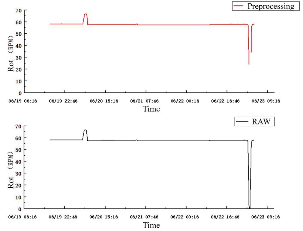
Basic statistics of the samples before and after preprocessing are summarized in

Table 3. Basic information of samples.

Feature	Basic Information
Data start and end time	06:20 on 9 June 2020–08:10 on 14 May 2021
Number of samples	43,186
Sampling interval	10 min

. As illustrated in Figure 2, the red curve representing the preprocessed data has successfully removed the abnormal data points below the minimum stable speed from the original black raw-data curve.

3.2. Steady-State Operating Region Identification

Various navigation states of a ship generate a large amount of non-steady-state data, which can interfere with the performance evaluation of the marine main engine. The steady-state detection (SSD) algorithm proposed by Kelly et al. [10] requires few manually set parameters and is suitable for multivariate steady-state detection, making it well suited for identifying the stable operating intervals of a marine main engine.

In this study, the SSD algorithm from reference [10] is adopted to identify stable intervals, with two parameters to be specified.

The first parameter is the window width $n$. If $n$ is too small, the detection process may not provide sufficient time to reach a steady state; if $n$ is too large, unstable data within the window might be misclassified as steady. Therefore, the window size should be chosen according to the actual operating characteristics of the target engine. In this paper, the window width is set to $n=12$, corresponding to a 2 h duration under the 10 min sampling interval. This setting matches the operating transition law of large low-speed marine diesel engines. Constrained by operating procedures and cylinder thermal stress, the transition of main engine parameters from one steady state to another typically takes 1–2 h under high-load ocean-going conditions. Taking into account the thermal inertia of lubricating oil and cylinder liner cooling water, the overall steady-state transition process is basically consistent with this window length, which can avoid misclassifying normal transitional fluctuations as anomalies. Fast condition switches under low loads belong to port maneuvering non-steady-state scenarios, which are inherently excluded in the steady-state detection step.

The second parameter is the critical value of the Student’s $t$-test, which is determined by looking up the table according to the degrees of freedom $v$ and the significance level α. In this study, the significance level is set to 0.025, which was chosen by tuning on the real-ship dataset, within the tunable range suggested by literature [10]. The degrees of freedom refer to the number of independent or freely varying parameters in a sample when using sample statistics to estimate population parameters. The formula for the degrees of freedom of the independent Student’s $t$-test is as follows:

$$v=n-2$$

(6)

where $n$ represents the number of samples, i.e., the window width.

Thus, by determining whether the relevant thermal parameters at a given time are in a steady state, it can be judged whether the marine main engine is operating stably. The sample information after steady-state identification is presented in

Table 4. Basic information of samples after steady-state identification.

Feature	Basic Information
Data start and end time	03:00 on 14 June 2020–07:40 on 14 May 2021
Number of samples	37,026
Sampling interval	10 min

.

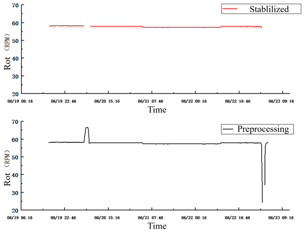
Figure 3 shows the rotational speed before and after SSD steady-state detection. The black curve corresponds to the preprocessed data, and the red curve corresponds to the data after steady-state detection. The two large fluctuations in the preprocessed series correspond to acceleration, deceleration, or shutdown transients and are excluded from the steady-state dataset. The resulting series is more suitable for performance comparative analysis under stable operating conditions.

3.3. Operating Condition Classification

CLIQUE (Clustering In QUEst) is a grid- and density-based clustering method for high-dimensional spaces. It partitions each selected dimension into grid intervals, identifies dense units, and connects adjacent dense units into clusters. This formulation is suitable for unlabeled operating data because the condition regions are determined from data density rather than a preassigned class label.

The CLIQUE procedure follows the established grid-density formulation [21,23]. A unit is dense when the fraction of samples it contains exceeds the density threshold τ and connected dense units form a cluster.

The detailed procedure for partitioning the marine main engine operating conditions using the CLIQUE algorithm is described below:

• Determine the dimensionality of the multidimensional space according to the number of performance parameters required for condition partitioning.
• Set the grid segmentation separately for each dimension, using the numbers of intervals reported in

  Table 5. Grid ranges and segmentation of the five CLIQUE input dimensions.

  Grid Dimension	Minimum	Maximum	Number of Segments
  Fuel type	1	4	8
  Speed/RPM	20	80	240
  Power/kW	0	20,000	500
  Scavenging temperature/°C	20	80	240
  Scavenging pressure/MPa	0	0.6	60

  .
• When k = 1, all rectangular units are candidate dense units.
• Traverse the multidimensional space and count the number of data points contained in each dense unit within the k-dimensional subspace, i.e., compute its density.
• Identify all dense units in the k-dimensional subspace according to the density threshold τ.
• Eliminate unqualified dense subspaces.
• Determine the set of candidate dense units for the (k + 1)-dimensional subspace based on the dense unit set of the k-dimensional subspace; if the dense units of the (k + 1)-dimensional subspace are empty, proceed to the next step; otherwise, jump back to step (4).
• Identify the clusters in the k-dimensional space.
• Save the clustering information to the database.

The 37,026 samples retained after steady-state screening are used for operating condition partitioning. Five variables—fuel type, power, rotational speed, scavenge air temperature and scavenge air pressure—define the CLIQUE input space. The remaining 17 variables are carried as performance monitoring parameters. For subsequent outlier detection via Mahalanobis distance calculation after condition partitioning, all 22 variables are used, including the five partitioning variables and the 17 monitoring parameters. Table 5 reports the range and grid segmentation for each CLIQUE input dimension.

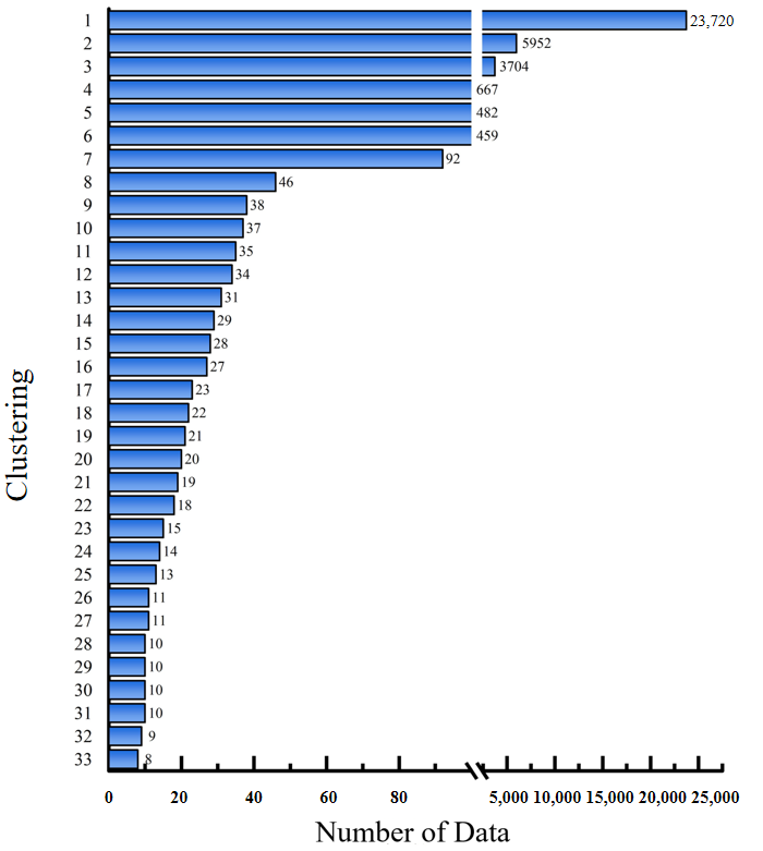
The density threshold is τ = 0.002. With 37,026 steady samples, a grid unit is dense when it contains approximately 74 or more samples. This density-based criterion is distinct from conventional engineering verification methods based on an absolute speed difference. Using the grid settings in Table 5, CLIQUE identifies 33 operating condition clusters (Figure 4). Condition 1 contains 23,720 samples and is the most populated cluster; Condition 33 contains eight samples, representing a rare transient operating condition.

To quantitatively evaluate the performance of CLIQUE in operating condition partitioning and clarify the rationale for algorithm selection, the classic K-means++ algorithm is adopted for a matched-data comparison. The clustering experiment is conducted on the same 37,026 steady-state samples with the same five operating condition variables. Since K-means++ is a distance-based clustering algorithm, min–max normalization is performed on the input variables before clustering. The optimal number of clusters k is determined by the silhouette coefficient, which measures the intra-cluster cohesion and inter-cluster separation of the clustering results.

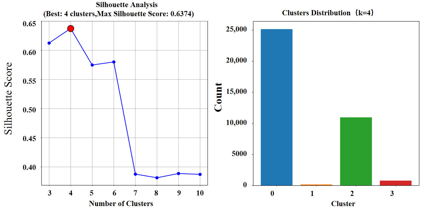
Figure 5 presents the silhouette coefficient curve across k = 3 to 10 and the sample size distribution under the optimal four-cluster solution. The algorithm achieves the maximum silhouette coefficient of 0.6374 at k = 4. The cluster distribution panel shows that the partitioning result is dominated by one large-scale cluster and one medium-sized cluster, accompanied by two small clusters, representing a relatively coarse global partition of the operating space.

Table 6. Matched-data comparison of K-means++ and CLIQUE for operating condition partitioning.

Criterion	K-Means++	CLIQUE	Comparative Interpretation
Input	37,026 steady samples; five normalized variables	The same 37,026 samples and five variables	Matched-data baseline
Cluster-number rule	k searched and fixed at 4	No preset k; connected dense units define clusters	CLIQUE imposes less prior structural constraint
Reported result	4 clusters; maximum silhouette coefficient = 0.6374	33 clusters; largest = 23,720 samples; smallest = 8	CLIQUE provides finer local operating condition resolution
Cluster geometry	Distance-to-centroid Voronoi partition	Grid- and density-connected regions	CLIQUE better accommodates irregular and sparse operating zones
Workflow role	Coarse global grouping	Fine condition screening	CLIQUE is better suited to this workflow
Validity caveat	Silhouette coefficient reported	Silhouette coefficient not calculated	The conclusion is task-specific, not universal

systematically summarizes the multidimensional comparison between K-means++ and CLIQUE. Considered alongside the 33-condition CLIQUE result in Figure 4, the difference in partition granularity is distinct: K-means++ compresses the operating space into four centroid-based Voronoi partitions, while CLIQUE identifies 33 density-connected operating condition clusters using the density threshold τ = 0.002 and variable-specific grid resolution, retaining a much finer set of both common and sparse local conditions.

In terms of underlying mechanism, K-means++ requires the number of clusters to be pre-specified and produces convex cluster boundaries based on centroid distance. In contrast, CLIQUE does not rely on a pre-defined cluster count, and clusters are formed by connecting adjacent dense grid units, which can better adapt to the irregular shape and uneven sample distribution of marine engine operating conditions. For the core objective of this study—isolating locally comparable operating regions before Mahalanobis distance-based performance evaluation—CLIQUE demonstrates task-specific advantages over K-means++, rather than general algorithmic superiority.

As noted above, this task-specific advantage should not be interpreted as universal algorithmic superiority. The silhouette coefficient is adopted as the validity metric for K-means++, while it is not calculated for the CLIQUE result in this study. The two partitioning approaches are not ranked under a unified general validity index, and the algorithm selection is based on the specific demand of fine-grained operating condition partitioning for marine main engine performance analysis.

3.4. Condition-Specific Multivariate Deviation and Retrospective Change-Point Analysis

3.4.1. Full-Condition Deviation Distribution and Analysis

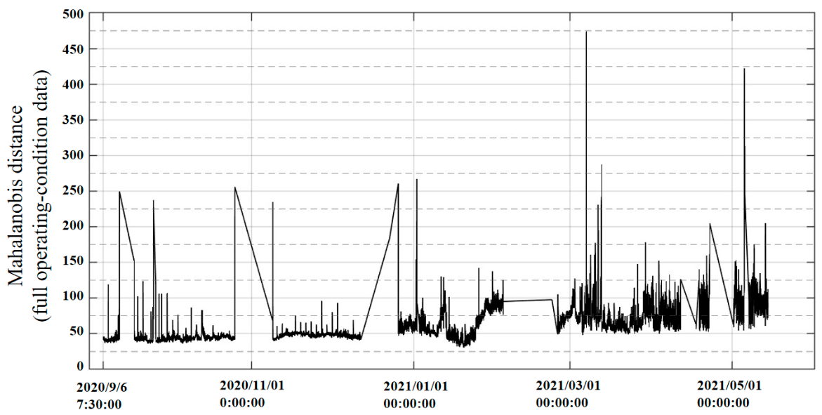
Based on the partitioning results of 33 steady-state operating conditions obtained by the CLIQUE algorithm, this section conducts condition-specific multivariate deviation analysis and retrospective change-point detection. To visually demonstrate the degree of interference caused by operating condition shifts on performance deviation calculation, the Mahalanobis distance of each steady-state sample relative to its corresponding condition centroid is calculated for the full dataset, and the time series distribution of deviations across all operating conditions is derived, as shown in Figure 6.

From the perspective of overall distribution, the Mahalanobis distance presents significant step-like fluctuations with the switching of operating conditions, and there are notable differences in the distance baseline across different operation phases: the distance baseline under high-load conditions is generally higher than that under low-load conditions, and sharp jumps in distance values occur during condition transition periods. If performance evaluation and change-point detection are performed directly across operating conditions on the full dataset, the parameter distribution shifts caused by operating condition differences will be misinterpreted as equipment performance changes, introducing large systematic deviations into the analysis results.

3.4.2. Condition-Specific Multivariate Deviation and Analysis

Since Condition 1 is the most frequently observed cluster, it is selected as the common operating condition for the case study. It contains 23,720 samples from 19:00 on 7 July 2020 to 07:40 on 14 May 2021. This frequency-based designation does not imply that the condition is optimal or independently verified as healthy.

Table 7. Parameter ranges for the selected Condition 1.

Parameter Category	Parameter	Range
Input dimension parameters	Fuel type	LSHFO
	Power/kW	10,520–12,240
	Speed/RPM	57.5–58.75
	Scavenging temperature/°C	46.75–52
	Scavenging pressure/MPa	0.07–0.1
Output dimension parameters	Exhaust gas temperature of cylinder #1/°C	352.71–361.28
	Exhaust gas temperature of cylinder #2/°C	350.05–360.57
	Exhaust gas temperature of cylinder #3/°C	351.51–361.32
	Exhaust gas temperature of cylinder #4/°C	346.1–356.28
	Exhaust gas temperature of cylinder #5/°C	355.71–363.86
	Exhaust gas temperature of cylinder #6/°C	353.67–361.62
	Lubricating oil inlet temperature/°C	45.19–46.34
	1# Cylinder liner cooling water outlet temperature/°C	88.29–89.69
	2# Cylinder liner cooling water outlet temperature/°C	88.21–89.87
	3# Cylinder liner cooling water outlet temperature/°C	87.86–89.31
	4# Cylinder liner cooling water outlet temperature/°C	88.02–89.37
	5# Cylinder liner cooling water outlet temperature/°C	88.6–90.01
	6# Cylinder liner cooling water outlet temperature/°C	88.32–89.74
	Cylinder liner cooling water inlet pressure/MPa	0.4685–0.4791
	Fuel flow rate/(kg/h)	1935.52–2022.81
	Specific fuel oil consumption/(g/kW·h)	172.42–182.04
	Cylinder liner cooling water inlet temperature/°C	84.05

summarizes its parameter ranges.

After the operating conditions of the main engine are partitioned using the CLIQUE clustering algorithm, the Mahalanobis distance of performance samples at different time points under the same operating condition is calculated, yielding a time series of Mahalanobis distance.

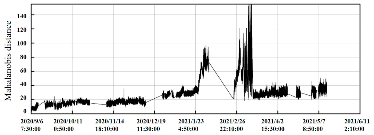
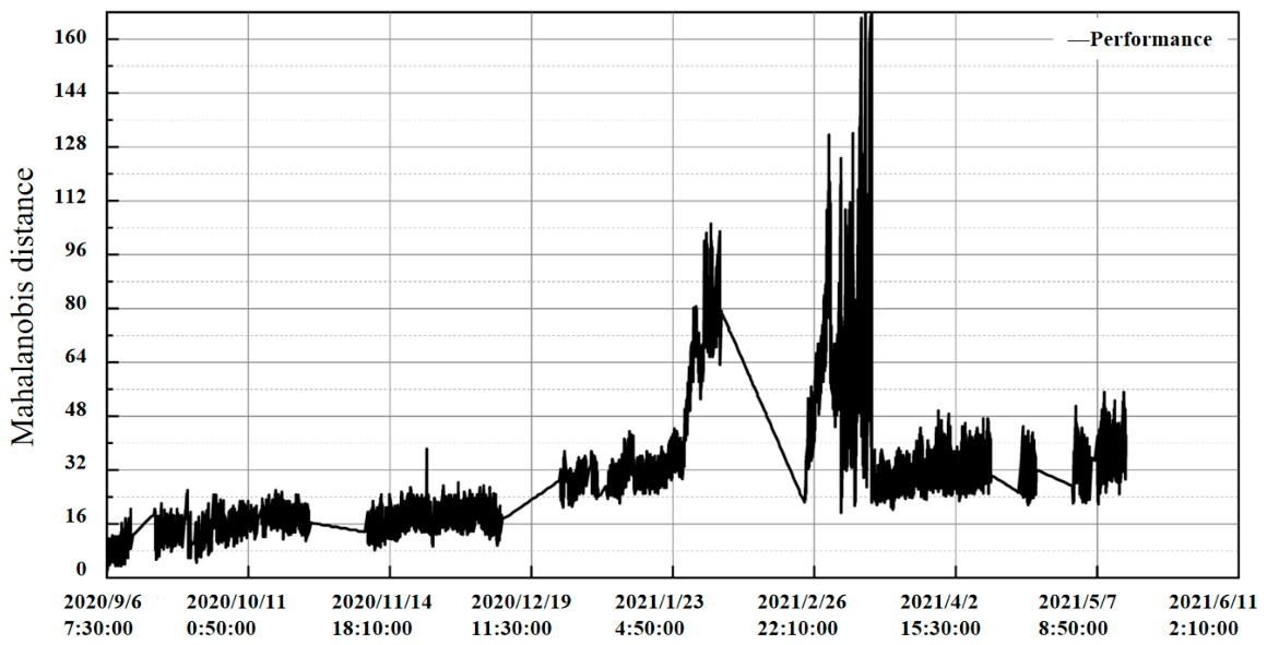
Taking the common operating range Condition 1 as an example, the overall performance of the marine main engine is evaluated and analyzed. The first 1000 performance samples are selected as the initial performance baseline sample space. Since these samples correspond to the period immediately following scheduled docking repair and system commissioning, they are treated as representing the healthy state under an engineering assumption. Their mean values are listed in

Table 8. Rounded mean values of the initial reference set for Condition 1.

Performance Parameter	Mean Value
Cylinder liner cooling water inlet temperature/°C	83.773
1# Cylinder liner cooling water outlet temperature/°C	89.697
2# Cylinder liner cooling water outlet temperature/°C	89.846
3# Cylinder liner cooling water outlet temperature/°C	89.163
4# Cylinder liner cooling water outlet temperature/°C	89.092
5# Cylinder liner cooling water outlet temperature/°C	89.834
6# Cylinder liner cooling water outlet temperature/°C	89.517
Cylinder liner cooling water inlet pressure/MPa	0.473
Exhaust gas temperature of cylinder #1/°C	358.572
Exhaust gas temperature of cylinder #2/°C	352.283
Exhaust gas temperature of cylinder #3/°C	351.790
Exhaust gas temperature of cylinder #4/°C	343.937
Exhaust gas temperature of cylinder #5/°C	356.397
Exhaust gas temperature of cylinder #6/°C	352.382
Lubricating oil inlet temperature/°C	45.545
Scavenging air temperature/°C	51.233
Scavenging air pressure/MPa	0.084
Speed/RPM	58.234
Power/kW	11,815.6
Fuel flow rate/(kg/h)	2035.41
Specific fuel oil consumption/(g/kW·h)	172.32
Fuel type	3

, spanning from 19:00 on 7 July 2020 to 7:20 on 6 September 2020. Subsequently, the Mahalanobis distance between performance samples at different time instants and the initial sample space is computed, resulting in a Mahalanobis distance time series of length 22,720. The corresponding Condition-specific multivariate deviation trajectory is shown in Figure 7.

As shown in Figure 7, the Mahalanobis distance gradually increases from September 2020 to late January 2021, which is consistent with the empirical gradual deviation pattern of marine main engine performance under normal operating conditions. However, from mid-January to March 2021, the Mahalanobis distance exhibits an abrupt rise and pronounced fluctuations, indicating an obvious deviation of the main engine’s overall operating state from the baseline. After March 2021, the growth of the Mahalanobis distance slows down, suggesting that the deviation rate reverts to a normal level.

It can be preliminarily inferred from the data trajectory that abnormal performance conditions may have occurred during the period from mid-January to March 2021, which could be related to potential anomalies or performance fluctuations. The subsequent recovery of the deviation trend is likely associated with anomaly rectification or maintenance adjustments. Nevertheless, these inferences are drawn purely from data-driven deviation analysis, and the specific causes require further verification with independent operation and maintenance records.

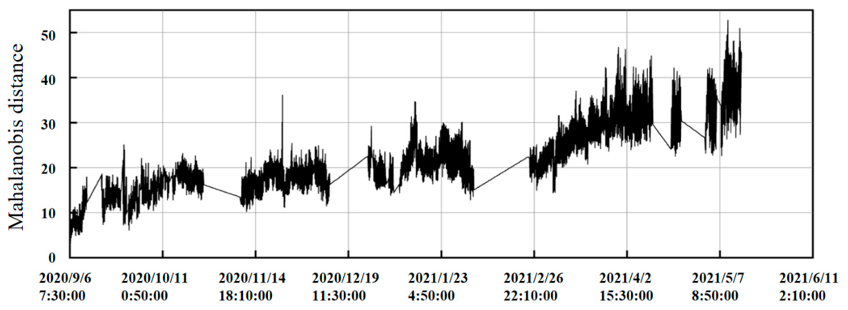
To verify this hypothesis, ablation experiments are conducted by sequentially excluding each performance parameter, recalculating the Mahalanobis distance and fitting the performance deviation trend curve. The results show that, when the parameter “2# Cylinder liner cooling water outlet temperature” is excluded, the fitted deviation curve evolves smoothly over time with no abrupt jumps or severe fluctuations (see Figure 8). In contrast, removing any other performance parameter does not alter the deviation pattern, which remains consistent with the full-parameter trajectory in Figure 9. Further analysis confirms that the 2# Cylinder liner cooling water outlet temperature exhibits significant fluctuations from late February to March 2021 (see Figure 10), which matches the abrupt deviation period observed in the full-parameter curve, indicating that the main engine may have experienced an operational anomaly during this period. The ablation experiment identifies the 2# cylinder liner cooling water outlet temperature as the parameter most strongly associated with the multivariate deviation; nonetheless, the physical location and root cause of any fault cannot be determined from the available data without independent maintenance records.

3.4.3. Retrospective Change-Point Analysis

The core objective of anomaly early warning is to issue an alert signal before the anomaly fully develops. However, in real navigation scenarios, if the warning is triggered only after an obvious change in the performance deviation trend has already occurred, the optimal intervention opportunity is often missed. To address this issue, an anomaly early warning technique based on time-domain analysis is proposed in this study. The core idea is to identify the first occurrence of a sudden change (mutation) in the performance deviation curve of the marine main engine as the anomaly warning timing while simultaneously localizing the abnormal cause, thereby achieving proactive anomaly prevention. It should be noted that the present analysis is retrospective (post hoc): the proposed pipeline is applied to historical voyage data to estimate the lead time, rather than deployed as a real-time online warning system.

In this paper, the cumulative anomaly curve method and the Yamamoto-type signal-to-noise ratio (SNR) rule [24] are employed to detect mutations in the Mahalanobis distance time series. The cumulative anomaly method calculates the cumulative anomaly value at each time point in the time series and generates a curve with time as the abscissa, which is used to intuitively visualize the trend. The rise and fall of the curve reflect the increase or decrease in the anomaly, and the approximate time of a mutation in the target time series can be identified by changes in the curve trend [24,25]. For a time series X, the cumulative anomaly at a given time $t$ is expressed as:

$$x_t={\displaystyle \sum _{i=1}^t}(x_i-\overline{x})$$

(7)

where $\overline{x}$ is the mean of the series X.

The Yamamoto-type SNR rule evaluates whether a mutation occurs at a given point by comparing the means of two sub-sequences. It should be noted that this SNR threshold is an empirical heuristic gate rather than a p-value significance test; no significance level α or p-value is computed by the rule itself. The basic idea is to treat the problem of whether there is a significant difference between the means of two sub-sequences in a time series as the problem of whether there is a significant difference between the means of two populations. Suppose a series X, and the numbers of samples in the sub-sequences before and after the test point are $n_1$ and $n_2$, respectively. The signal-to-noise ratio (SNR) is defined as:

$$SNR={\displaystyle \frac{|\overline{x_1}-\overline{x_2}|}{s_1+s_2}}$$

(8)

where $\overline{x_1}$ and $\overline{x_2}$ are the means of the preceding and succeeding sub-sequences and $s_1$ and $s_2$ are their respective standard deviations.

SNR > 1.0 is treated as evidence of a candidate mutation, and SNR > 2.0 is treated as evidence of a sharp mutation. Since the test statistic relies on a sub-sequence of data collected after the test point, the score at any candidate time point requires subsequent observations to compute. For prospective online deployment, a one-sided or sequential detection rule would be required, with dedicated evaluation of detection delay and false alarm rate.

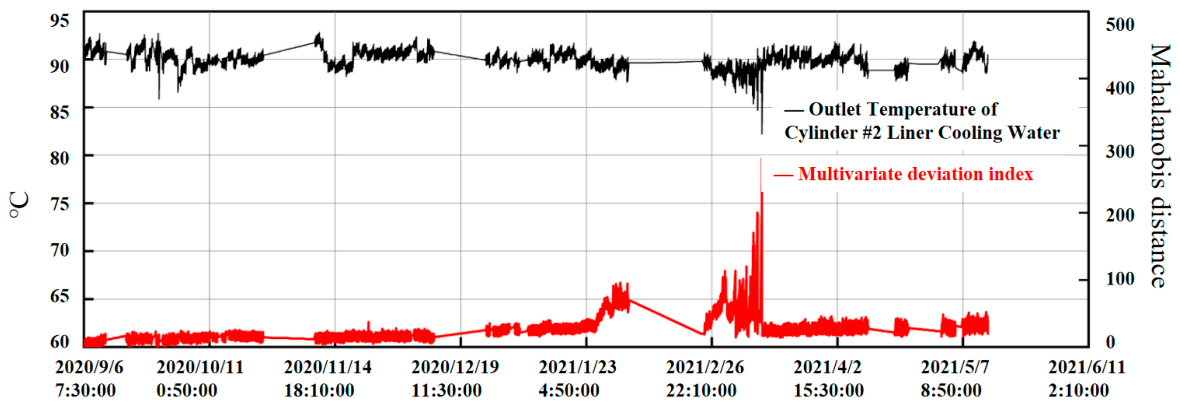
In the historical dataset, the 2# Cylinder liner cooling water outlet temperature becomes visibly more volatile after the multivariate deviation trajectory begins to shift (Figure 11). This temporal sequence supports the retrospective mutation analysis but does not constitute validated evidence of a prospective early warning lead time.

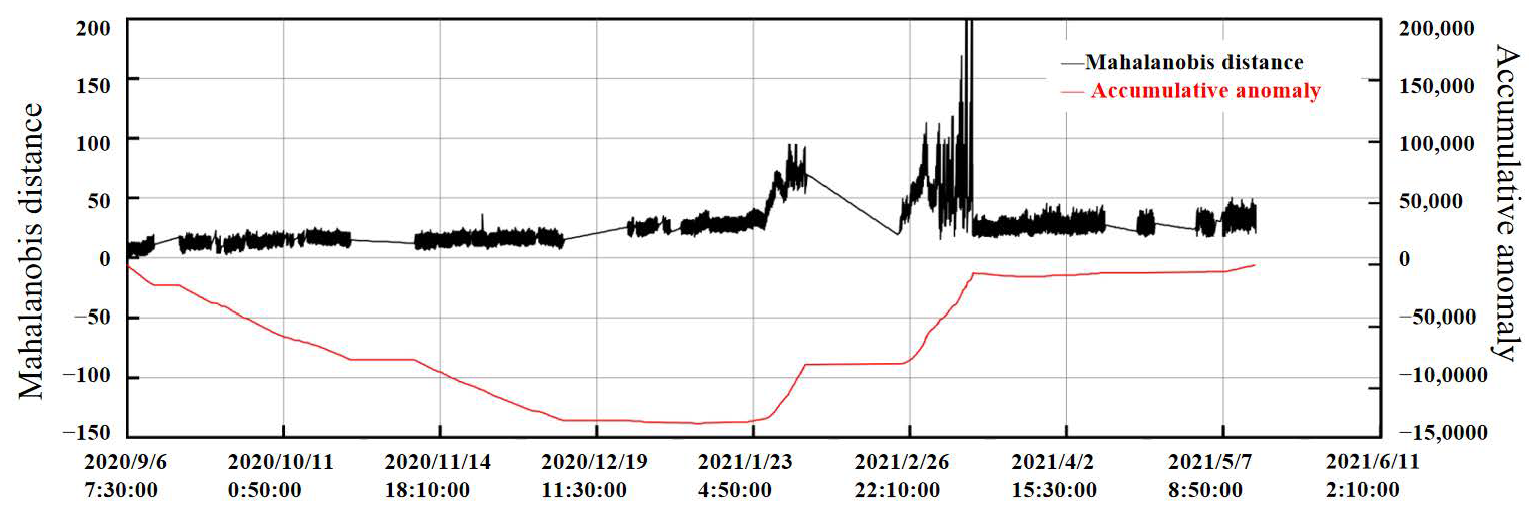
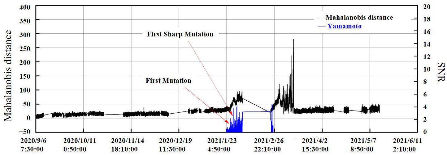
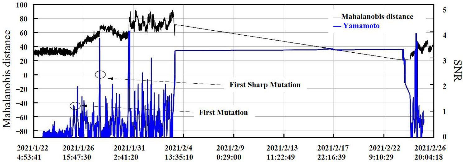
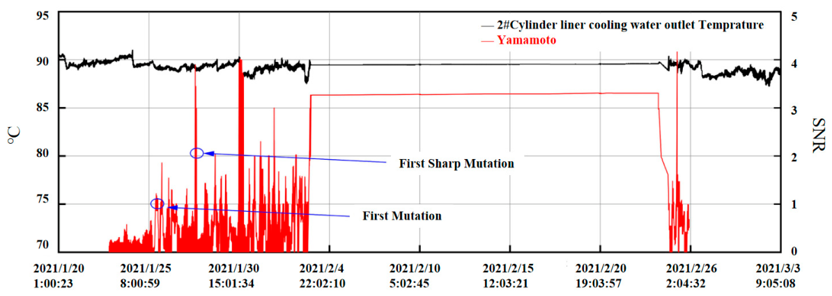
To identify the specific mutation time using time-domain analysis, the cumulative anomaly method is first employed to determine the approximate time range of the mutation, and then, the Yamamoto test is used for precise localization. The trend of the cumulative anomaly curve can intuitively reveal the approximate time of the mutation in the performance deviation curve. From Figure 12, it can be observed that, as time increases, the Mahalanobis distance gradually rises, and the corresponding cumulative anomaly value gradually decreases, which is consistent with the general pattern of gradual performance degradation in marine main engines. However, in late January 2021, the cumulative anomaly curve shows a clear upward trend, indicating a mutation in the performance deviation curve. Thus, it can be determined that the first mutation of the performance deviation curve roughly occurred between 23 January and 26 February 2021. The performance series corresponding to this time period is extracted, and the Yamamoto test is applied to calculate the SNR, with the resulting mutation test curves shown in Figure 13 and Figure 14.

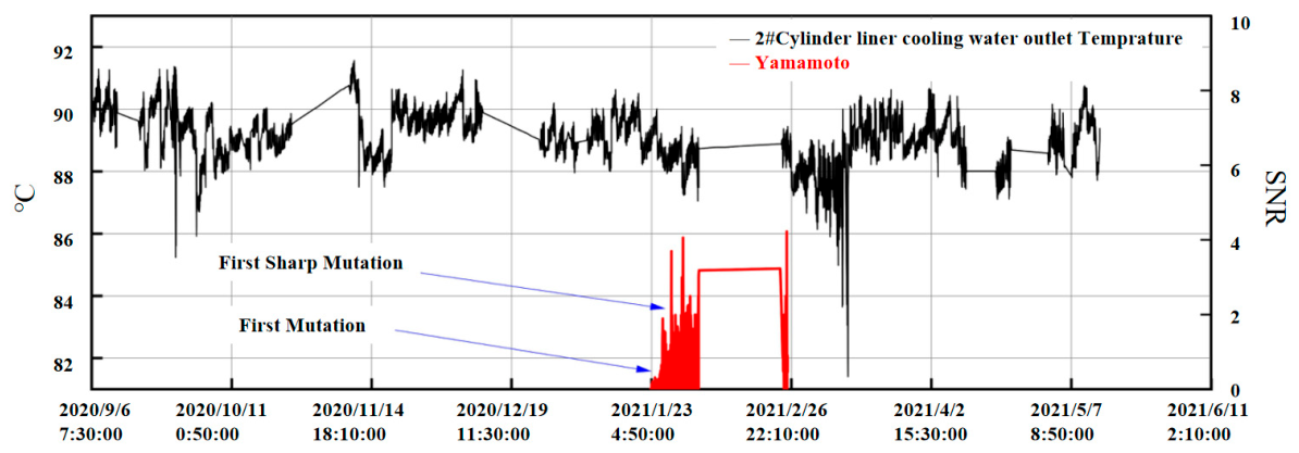
As can be seen in Figure 13 and Figure 14, at 18:10 on 25 January 2021, the SNR first exceeds 1.0, confirming that the exact time of the first mutation in the performance deviation curve is 18:10 on 25 January 2021. Since both the cumulative anomaly calculation and the Yamamoto test rely on observations after each candidate time point, this timestamp corresponds to a retrospectively detected mutation point rather than a real-time warning decision generated using only data available up to time t. This point marks the recommended retrospective reference point for anomaly early warning.

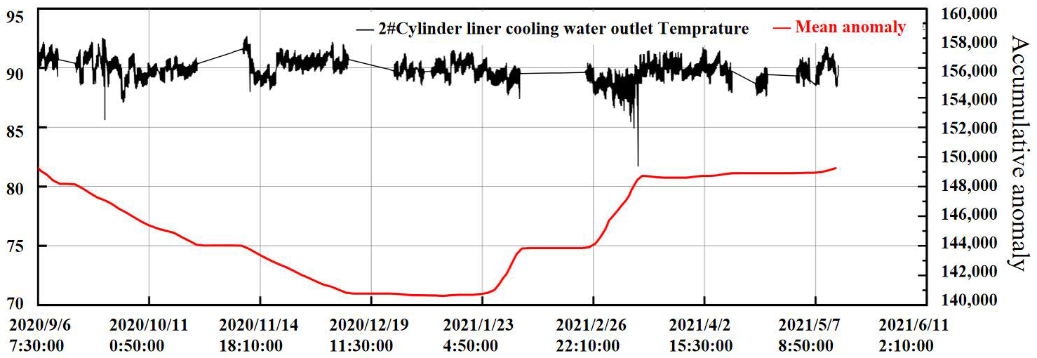
A comparative analysis between the curves and the temperature parameter is shown in Figure 15, Figure 16 and Figure 17. It can be observed that there is still a considerable interval between the first mutation time of the overall performance deviation curve and the occurrence of significant abnormal fluctuation of the temperature parameter, which further demonstrates the early detection potential of the proposed anomaly early warning method.

4. Conclusions

This paper proposes a data-driven performance evaluation framework for marine main engines, which employs the Mahalanobis distance as a quantitative performance metric and effectively reveals the performance deviation trend of the main engine under steady operating conditions. Furthermore, by analyzing the performance deviation curve, retrospective identification of performance anomalies is achieved. The results demonstrate that the proposed method can identify subtle performance changes and trigger statistical alerts before any single monitoring parameter of the main engine exhibits obvious abnormal fluctuations. The specific conclusions are as follows:

• Using nearly one year of monitoring data comprising 43,186 samples from the marine main engine, 37,026 steady-state samples were obtained after data preprocessing and steady-state screening. Through the CLIQUE clustering algorithm, the samples were partitioned into 33 operating condition clusters, among which Condition 1 (containing 23,720 samples) was identified as the common operating range of the main engine. Comparative experiments with the classical K-means++ clustering algorithm verify that the CLIQUE algorithm can automatically partition the main engine operating conditions without pre-defining the number of clusters and achieve fine-grained quantitative classification of these conditions with better adaptability to the non-uniform distribution of actual marine engine operating conditions.
• For the samples in the common operating range, the Mahalanobis distance was calculated, and the corresponding performance deviation curve was constructed. This curve followed the typical gradual deviation pattern under normal operating conditions in the early stage, while obvious mutations and fluctuations appeared in the latter stage, indicating potential performance anomalies. Through ablation experiments that sequentially excluded individual monitoring parameters, the 2# Cylinder liner cooling water outlet temperature was identified as the parameter most strongly correlated with the overall multivariate deviation; further time series analysis of this parameter also corroborated the presence of abnormal fluctuations during the corresponding period.
• By comparing the variation curve of the 2# Cylinder liner cooling water outlet temperature with the overall performance deviation curve, it is found that the mutation in the performance deviation curve precedes the significant fluctuation of the temperature parameter by approximately 20 days, which indicates the potential to reserve a time buffer for anomaly early warning in retrospective analysis.

In summary, the performance evaluation and anomaly early warning framework proposed in this paper not only provides a new technical reference for the condition-based maintenance of marine main engines but also offers feasible research ideas for operating state classification and mutation detection of intelligent marine equipment.

Notably, this study still has certain limitations. First, the verification is conducted based on the measured data of a single marine main engine, and the generalizability of the method across different engine types and operating scenarios remains to be further verified. Second, the current analysis is a retrospective study based on full historical data, and the actual performance of the method in prospective online deployment needs to be further validated with engineering practice. Third, there is a lack of independent maintenance records or inspection reports as ground truth to confirm the physical cause of the detected statistical anomaly, and the correspondence between multivariate statistical deviation and actual physical faults requires further investigation.

In future work, more conventional thermal and pressure parameters will be introduced to achieve a more comprehensive characterization of the overall operating state of the marine main engine. In addition, multi-engine validation and prospective online deployment testing will be carried out to further improve the engineering applicability of the proposed framework.

References

1. Mauro, F.; Kana, A.A. Digital twin for ship life-cycle: A critical systematic review. Ocean Eng. 2023, 269, 113479. [Google Scholar] [CrossRef] [Scilit]
2. Ahn, Y.G.; Kim, T.; Kim, B.R.; Lee, M.K. A study on the development priority of smart shipping items—Focusing on the expert survey. Sustainability 2022, 14, 6892. [Google Scholar] [CrossRef] [Scilit]
3. Chen, W.Y.; Xin, B.; Zhu, Z.Q. Real-time collision avoidance for unmanned ships under constraints of rules. In Proceedings of the 2019 IEEE 16th International Conference on Networking, Sensing and Control (ICNSC 2019), Banff, AB, Canada, 9–11 May 2019; pp. 80–85. [Google Scholar] [CrossRef] [Scilit]
4. Hu, Y.; Miao, X.W.; Si, Y.; Pan, E.S.; Zio, E. Prognostics and health management: A review from the perspectives of design, development and decision. Reliab. Eng. Syst. Saf. 2022, 217, 108063. [Google Scholar] [CrossRef] [Scilit]
5. Hou, W.K.; Yan, J.F.; Yao, G.P. A comprehensive validation approach of PHM system’s diagnosis and verification. In Proceedings of the 2014 Prognostics and System Health Management Conference (PHM-2014 Hunan), Zhangjiajie, China, 24–27 August 2014; pp. 199–202. [Google Scholar] [CrossRef] [Scilit]
6. Liu, Z.C.; Zhang, C.X.; Dong, E.Z.; Wang, R.C.; Li, S.Y.; Han, Y.M. Research progress and development trend of prognostics and health management key technologies for equipment diesel engine. Processes 2023, 11, 1972. [Google Scholar] [CrossRef] [Scilit]
7. Zhan, Y.; Zeng, J. Implementation of intelligent operation and maintenance for ships supported by big data. J. Shanghai Marit. Univ. 2019, 40, 62–66. (In Chinese) [Google Scholar]
8. Raissi, M.; Perdikaris, P.; Karniadakis, G.E. Physics-informed neural networks: A deep learning framework for solving forward and inverse problems involving nonlinear partial differential equations. J. Comput. Phys. 2019, 378, 686–707. [Google Scholar] [CrossRef] [Scilit]
9. Narasimhan, S.; Kao, C.S.; Mah, R.S.H. Detecting changes of steady states using the mathematical theory of evidence. AIChE J. 1987, 33, 1930–1932. [Google Scholar] [CrossRef] [Scilit]
10. Kelly, J.D.; Hedengren, J.D. A steady-state detection (SSD) algorithm to detect non-stationary drifts in processes. J. Process Control 2013, 23, 326–331. [Google Scholar] [CrossRef] [Scilit]
11. Liu, B.; Gan, H.; Chen, D.; Shu, Z. Research on fault early warning of marine diesel engine based on CNN-BiGRU. J. Mar. Sci. Eng. 2023, 11, 56. [Google Scholar] [CrossRef] [Scilit]
12. Su, Y.; Gan, H.; Ji, Z. Research on multi-parameter fault early warning for marine diesel engine based on PCA-CNN-BiLSTM. J. Mar. Sci. Eng. 2024, 12, 965. [Google Scholar] [CrossRef] [Scilit]
13. Zhang, B.S.; Zhang, L.; Zhang, B.; Yang, B.; Zhao, Y. A fault prediction model of adaptive fuzzy neural network for optimal membership function. IEEE Access 2020, 8, 101061–101067. [Google Scholar] [CrossRef] [Scilit]
14. Perera, L.P.; Mo, B. Data analysis on marine engine operating regions in relation to ship navigation. Ocean Eng. 2016, 128, 163–172. [Google Scholar] [CrossRef] [Scilit]
15. Vanem, E.; Brandsæter, A. Unsupervised anomaly detection based on clustering methods and sensor data on a marine diesel engine. J. Mar. Eng. Technol. 2019, 20, 217–234. [Google Scholar] [CrossRef] [Scilit]
16. Liu, Y.; Huang, L.; Sun, P.; Ma, R. Performance evaluation method for marine main diesel engines based on ship trial data. Trans. CSICE 2018, 36, 182–190. (In Chinese) [Google Scholar]
17. Zheng, Q.; Lin, J.; Zhao, Z.; Yu, W. Performance evaluation of frequent operating zones of marine main engine based on cluster analysis. J. Quanzhou Norm. Univ. 2021, 39, 34–39. (In Chinese) [Google Scholar]
18. Perera, L.P.; Mo, B. Marine engine-centered data analytics for ship performance monitoring. J. Offshore Mech. Arct. Eng. 2017, 139, 021301. [Google Scholar] [CrossRef] [Scilit]
19. Zhang, J.; Hu, D.; Yang, T.; Zhou, H.; Li, X. A time series and deep fusion framework for rotating machinery fault diagnosis. Eng. Appl. Artif. Intell. 2024, 128, 107456. [Google Scholar] [CrossRef] [Scilit]
20. Je-Gal, H.; Lee, S.-J.; Yoon, J.-H.; Lee, H.-S.; Yang, J.-H.; Kim, S. A novel time–frequency feature fusion approach for robust fault detection in a marine main engine. J. Mar. Sci. Eng. 2023, 11, 1577. [Google Scholar] [CrossRef] [Scilit]
21. Ma, F.; Wang, C.; Huang, J.; Zhong, Q.; Zhang, T. Key grids based batch-incremental CLIQUE clustering algorithm considering cluster structure changes. Inf. Sci. 2024, 660, 120109. [Google Scholar] [CrossRef] [Scilit]
22. Fu, C.; Liang, X.; Li, Q.; Lu, K.; Gu, F.; Ball, A.D.; Zheng, Z. Comparative study on health monitoring of a marine engine using multivariate physics-based models and unsupervised data-driven models. Machines 2023, 11, 557. [Google Scholar] [CrossRef] [Scilit]
23. Deng, G.; Liu, C.; Xiong, Y. Research and implementation of CLIQUE clustering algorithm based on grid and density. Comput. Mod. 2008, 12, 8–11. (In Chinese) [Google Scholar]
24. Yamamoto, R.; Iwashima, T.; Sanga, N.K.; Hoshiai, M. An analysis of climatic jump. J. Meteorol. Soc. Jpn. 1986, 64, 273–281. [Google Scholar] [CrossRef] [Scilit] [PubMed]
25. Jiang, Y.; Xu, Z.; Wang, J. Comparative study of five trend detection methods based on annual runoff series. J. Hydraul. Eng. 2020, 51, 845–857. (In Chinese) [Google Scholar]
Figure 1. Variation curves of selected monitoring parameters.
Jmse 14 01665 g001
Figure 2. Trend variation of engine speed over a specific period after preprocessing.
Jmse 14 01665 g002
Figure 3. Trend changes in rotational speed after steady-state detection.
Jmse 14 01665 g003
Figure 4. Clustering information.
Jmse 14 01665 g004
Figure 5. K-means++ silhouette analysis and four-cluster sample distribution.
Jmse 14 01665 g005
Figure 6. Time series distribution of Mahalanobis distance across full operating conditions.
Jmse 14 01665 g006
Figure 7. Condition-specific multivariate deviation trajectory.
Jmse 14 01665 g007
Figure 8. Multivariate deviation trajectory after excluding the 2# Cylinder liner cooling water outlet temperature.
Jmse 14 01665 g008
Figure 9. Multivariate deviation trajectory after excluding the 1# Cylinder liner cooling water outlet temperature.
Jmse 14 01665 g009
Figure 10. 2# Cylinder liner cooling water outlet temperature trajectory.
Jmse 14 01665 g010
Figure 11. Comparison of the multivariate deviation index with the 2# Cylinder liner cooling water outlet temperature.
Jmse 14 01665 g011
Figure 12. Accumulated anomaly curve.
Jmse 14 01665 g012
Figure 13. Yamamoto test curve.
Jmse 14 01665 g013
Figure 14. Enlarged view of the abrupt change point in the Yamamoto test curve.
Jmse 14 01665 g014
Figure 15. Comparison of cumulative anomaly with the trend of 2# Cylinder liner cooling water outlet temperature.
Jmse 14 01665 g015
Figure 16. Comparison of Yamamoto-type SNR rule with the trend of 2# Cylinder liner cooling water outlet temperature.
Jmse 14 01665 g016
Figure 17. Enlarged view of the abrupt change point for comparison.
Jmse 14 01665 g017