Formation Reconfiguration for Underwater Gliders Under Ocean Current Disturbances: An Enhanced Distributed Model Predictive Control Algorithm

Abstract

Underwater glider (UG) formations exhibit significant trajectory deviations when subjected to non-uniform ocean currents, complicating spatial reconfiguration upon exiting complex marine environments and compromising environmental monitoring fidelity. To solve these problems, we develop a rapid formation reconfiguration algorithm based on distributed model predictive control (DMPC). The algorithm combines a flexible boundary-triggering mechanism for autonomous control suspension and rapid activation, a nonlinear vector heading pre-compensation scheme to counteract strong current disturbances, and a multi-objective leader capability assessment with a dynamic rotation strategy for optimized leader selection. The predictive plant model is calibrated utilizing empirical sea trial datasets, and its control performance is validated through comparative simulations against conventional MPC and active disturbance rejection control (ADRC). The results demonstrate that the proposed algorithm reduces the standard deviation of lateral inter-glider distance by 42% and 17% relative to ADRC and conventional MPC, shortens the reconfiguration time to 13.3 h, and lowers the maximum relative deflection, lateral distance standard deviation and average energy consumption. This framework significantly improves formation stability, reconfiguration efficiency, and energy efficiency, providing a robust methodology for persistent swarm deployments.

1. Introduction

Owing to their minimal acoustic signatures, extended operational endurance, and cost-effective deployment profiles, underwater gliders (UGs) have emerged as pivotal mobile nodes for deep-ocean environmental characterization and localized target tracking [1]; however, platform-generated mechanical noise degrades the data quality of onboard sonar systems, limiting their accuracy in acoustic detection applications [2]. Existing research has primarily suppressed mechanical noise through passive noise reduction methods, such as vibration isolation design and the application of damping materials [3,4,5], but it is challenging to eliminate such interference at the source. UGs operate in a low-actuation, low-sampling control mode within the designated silent zone. In this mode, the glider maintains a fixed net buoyancy and a static pitch angle, remaining in a balanced gliding state. Meanwhile, high-frequency distributed model predictive control (DMPC) online computation and frequent rudder surface actuations are halted to achieve concealment or energy saving. This intermittent control policy, however, introduces two fundamental technical challenges.

First, the formation is prone to disintegration when UGs operate silently within the silent zone. In the silent state, UGs cannot maintain formation coordination through communication devices. Gong et al. [6] established dynamic constraints among UG formation members using the potential field method, but the lack of real-time position sharing during silence makes the formation susceptible to disintegration due to ocean current disturbances or individual motion differences. Han et al. [7] further verified that with traditional PID control during communication interruption, the formation position root-mean-square error increases by 50.9%, indicating a significant rise in the risk of formation dispersal. To enhance formation stability, He et al. [8] were the first to introduce complex network theory into formation stability analysis, validating the robustness advantage of a diamond-shaped formation under strong ocean current disturbances by establishing a leader–follower dynamic model. However, existing methods mostly rely on global prior information about ocean currents; when facing unknown or dynamically changing current environments, the ability to maintain and rapidly reconfigure the formation still has significant limitations.

Second, ocean currents cause significant interference in a UG’s operational path. However, the spatiotemporal variation of ocean currents is complex, and their speed is comparable to a UG’s navigation speed, causing the actual path to deviate severely from the preset trajectory [9]. Jiang et al. [10] emphasized that ocean currents are the main interfering factor in formation path planning; especially in unknown or strongly dynamic flow fields, UGs may deviate from the target due to soaring energy consumption against currents or loss of control with currents. Simulations by Lan [11] showed that in the time-varying current environment of Tokyo Bay, the trajectory offset of traditional algorithms can reach up to 15% of the preset path length.

DMPC has become an important solution for formation control in complex environments due to its excellent performance in handling local constraints, dynamic coupling, and local communication of multi-agent systems [12]. Compared with the traditional centralized control architecture, DMPC decomposes the global optimization problem into local prediction tasks of multiple subsystems, which significantly reduces the computational burden and greatly enhances the flexibility and scalability of the system [13]. Recently, to address the challenge of limited communication resources, state-of-the-art studies have introduced a self-triggered mechanism, which dynamically adjusts the triggering frequency through prediction error feedback, effectively reducing redundant communication and conservatism of the control scheme [14]. Under non-ideal network conditions, DMPC further demonstrates its ability to cope with communication delays and random topology switching; for instance, the multi-objective optimization strategy systematically balances tracking accuracy and energy consumption [15]. In addition, for extreme disturbances such as denial-of-service attacks, DMPC with a resilient recovery mechanism has been proven to ensure string stability and closed-loop robustness of the formation [16]. These improved studies on communication robustness and computational efficiency provide valuable methodological references for solving the rapid formation reconfiguration of UGs after traversing ocean silent zones.

The effectiveness of formation control strategies highly depends on the fidelity of the dynamic model. Traditional UG models usually simplify the influences of deep-sea environmental variables, leading to non-negligible cumulative deviations in long-range motion prediction [17]. However, recent studies point out that since UGs are low-speed and weakly maneuverable vehicles, hull deformation caused by deep-sea high pressure and the resulting buoyancy loss are decisive factors affecting their motion characteristics [18]. The improved dynamic model constructed by introducing these environmental correction terms has been verified by sea trial data, whose mean absolute percentage error of prediction is reduced by approximately 44.54% compared with the conventional model, significantly improving the quantitative evaluation accuracy of motion performance [17]. Especially in non-uniform flow field environments, accurately modeling the flow field moment and its spatial vector components is crucial for analyzing the gliding efficiency and maneuvering stability of gliders [19]. This high-precision dynamic characterization provides a more reliable physical core for the rolling optimization of the DMPC algorithm, enabling the formation control system to more accurately predict and offset trajectory deviations caused by ocean current disturbances, thereby achieving efficient formation keeping and reconfiguration.

DMPC, leader–follower frameworks, event-triggered mechanisms, and leader rotation strategies have been widely explored for multi-agent formation control. However, existing approaches suffer from critical limitations when applied to UG formation control under complex marine conditions:

• Traditional MPC designs primarily target ideal communication and disturbance-free environments, lacking dedicated compensation for strong, time-varying ocean currents and adaptive logic for silent zone navigation, leading to severe trajectory divergence and formation disintegration;
• Conventional leader–follower methods rely on fixed leader assignments, resulting in uneven energy consumption across the formation and poor adaptability to dynamic marine disturbances;
• Static event-triggered schemes adopt fixed switching thresholds, failing to dynamically adjust control intensity based on real-time ocean current intensity and formation deviation, thus compromising reconfiguration efficiency and energy efficiency;
• Existing leader rotation strategies usually optimize only a single objective, ignoring the coupling of energy consumption, communication quality, and formation stability in complex marine scenarios.

To resolve these limitations, this paper introduces an enhanced control-oriented DMPC architecture characterized by the following methodological developments:

• We develop a nonlinear vector heading pre-compensation scheme that abandons the linear perturbation assumption of existing methods and analytically cancels cross-track velocity errors caused by strong currents, enabling stable formation control under extreme disturbance conditions that traditional DMPC cannot handle.
• We design an adaptive boundary-triggering mechanism based on the Reconfiguration Urgency Index (RUI), which replaces static thresholds with a disturbance-adaptive logic to realize autonomous control suspension in silent zones and rapid reactivation after exit; this outperforms conventional event-triggered strategies in balancing energy saving and reconfiguration speed.
• We propose a multi-objective leader evaluation and dynamic rotation strategy, which integrates energy, position, and communication indicators to optimize leader selection, breaking the single-objective limitation of existing rotation methods and achieving balanced energy distribution and robust formation stability.

The proposed algorithm combines the above innovations into a unified DMPC framework. The glider dynamic model and environmental parameters are calibrated using real sea trial data, while the formation control algorithm is validated through numerical simulations. It addresses the unique challenges of UG formations under ocean current disturbances and silent zone navigation, providing a practical solution for long-duration marine environmental monitoring.

2. UG Formation Modeling

2.1. Enhanced Dynamic Model Considering Ocean Environments

We first conduct dynamic modeling to analyze the relationship between UG motion characteristics and control inputs. First, dynamic analysis of the UG in the vertical plane is performed, establishing the inertial coordinate system (A-frame) and the body coordinate system (B-frame). The origin of the B-frame coincides with the buoyancy center point, and the origin of the A-frame coincides with a point on the sea surface. In the A-frame, the velocities of UGs along the axes are denoted as $u,y,w$, and the angular velocities along each axis in the B-frame are denoted as $p,q,s$ [20]. Figure 1 shows the schematic diagram of the force analysis of the UG.

The position conversion between the inertial frame and the body frame follows the following kinematic projection relation:

$$\left\{\begin{array}{l}\dot{x}=u\cos \theta +w\sin \theta \hfill \\ \dot{z}=-u\sin \theta +w\cos \theta \hfill \end{array}\right.$$

(1)

where $x,z$ denote the absolute position coordinates in the inertial frame; $u,w$ denote the axial velocity of the glider under the body frame; and $\theta$ represents the pitch angle.

Hydrodynamic drag $D$ and lift $L$ are the core forces dominating gliding motion, whose scalar magnitudes are determined by the relative flow velocity:

$$D={\displaystyle \frac{1}{2}}\rho V^{2}S{K}_D$$

(2)

$$L={\displaystyle \frac{1}{2}}\rho V^{2}S{K}_L$$

(3)

where $V$ is the relative gliding speed; $\rho$ is the seawater density; $S$ is the characteristic area of the hull; and $K_D$, $K_L$ are drag and lift coefficients calibrated via sea trial data. Under steady gliding conditions, lift and drag maintain force balance with buoyancy:

$$L=B\cos \xi$$

(4)

$$D=B\sin \xi$$

(5)

where $B$ denotes the net buoyancy of the UG, and $\xi$ stands for the glide angle of the UG. The horizontal and vertical navigation speeds of the glider relative to static seawater can be decomposed as

$$\left\{\begin{array}{l}\dot{X}=v_h=V\cos (\theta +\alpha )\hfill \\ \dot{Z}=v_z=V\sin (\theta +\alpha )\hfill \end{array}\right.$$

(6)

where $v_h$ and $v_z$ are the horizontal and vertical velocity components relative to static seawater, respectively, and $\alpha$ is the attack angle of the glider.

Classical underwater glider modeling further derives a set of highly coupled nonlinear differential equations based on rigid-body moment balance, mass-block dynamic equations, and analytical solutions of the attack angle and gliding angle. These full differential derivation formulas belong to mature basic theory and are not the core innovation of this paper; therefore, the complete complex derivation process is omitted here to avoid redundant content.

The standard ideal dynamic model ignores two key marine environmental interference factors, which lead to large long-term trajectory prediction errors in complex sea conditions. This paper improves the dynamic model by introducing two environmental correction terms: depth-dependent buoyancy attenuation and a spatially–temporally varying ocean current field, as detailed below.

First, as the dive depth $H$ increases, the variations in ambient temperature $T$ and hydrostatic pressure $P_e$ cause a thermo-mechanical contraction of the UG’s hull. Concurrently, seawater density ${\rho }_H$ exhibits spatial stratification. These hydrographic factors couple to produce a nonlinear buoyancy loss $\mathsf{\Delta }{B}_{\mathrm{loss}}(H)=\mathsf{\Delta }B-\mathsf{\Delta }B(H)$, which reduces the net driving buoyancy from its initial value $\mathsf{\Delta }B$ to the actual value $\mathsf{\Delta }B(H)$ at depth $H$. According to the improved UG modeling framework, this depth-dependent net driving buoyancy is quantified as

$$\mathsf{\Delta }B(H)=\left(V_0+\mathsf{\Delta }{V}_h(T,P_e)\right){\rho }_{h}g-V_0{\rho }_{0}g$$

(7)

where $V_0$ is the initial hull volume, ${\rho }_0$ is the reference seawater density at the sea surface, ${\rho }_h(H)$ is the seawater density at depth $H$ and $\mathsf{\Delta }{V}_h(T,P_e)$ denotes the hull deformation volume induced by thermo-mechanical coupling.

Second, the assumption of static water fundamentally limits trajectory prediction accuracy. When we introduce a three-dimensional ocean current velocity field $V_c={[u_c,v_c,w_c]}^T$, generated by the superposition of Lamb-type vortices and wind-driven currents, the ground velocity of the glider $V_g$ is the vector sum of its velocity relative to the fluid $V_r$ and the ocean current velocity $V_c$, i.e., $V_g=V_r+V_c$. Therefore, the effective relative velocity of the glider with respect to the fluid becomes $V_{\mathrm{eff}}=V_r=V_g-V_c$. Consequently, the hydrodynamic drag $F_R$ and lift $F_L$ formulated in Equations (4) and (5) must be dynamically updated based on $‖V_{\mathrm{eff}}‖$, fundamentally altering the force and moment equilibrium along all axes.

If the full high-fidelity nonlinear dynamic model is directly embedded into the DMPC prediction horizon, it will bring unacceptable online computing overhead and fail to meet the real-time requirement of multi-glider distributed cooperative control. To balance model precision and computational efficiency, this paper adopts a layered modeling strategy:

• A simplified linear nominal model calibrated by sea trial data is taken as the core rolling prediction model of DMPC, which will be discretized into state-space form in Section 3.1;
• All unmodeled environmental interferences, including depth buoyancy loss and ocean-current-induced disturbance moments, are aggregated into a unified lumped disturbance term, $D\left(k\right)$.

In the subsequent DMPC framework, a recursive disturbance observer is designed to estimate and compensate $D\left(k\right)$ in real time. Meanwhile, the nonlinear vector heading pre-compensation scheme proposed in Section 4 further counteracts steady-state trajectory deviation caused by strong currents, realizing a trade-off between high-precision environmental modeling and real-time distributed formation control.

2.2. Formation Kinematics Model Based on Leader–Follower

The principle of the traditional leader–follower method is to designate a leader vehicle and follower vehicles in the formation system, where the followers consistently maintain the formation by tracking the leader at preset distances and speeds to ensure stability [21]. However, UGs face challenges in achieving real-time communication, are prone to accumulated errors, and require a rapid response for formation reconfiguration after traversing silent zones, thus necessitating improvements to the traditional model. Inspired by the formation reconfiguration behavior observed in migratory geese [22], this study introduces a dynamic leader–follower framework. As shown in Figure 2, five UGs advance in a V-shaped formation, where ${\phi }_{LF}$ represents the heading angle difference between the leader and follower, and $l_{LF}$ denotes the distance between them.

Assuming $v^{\prime }$ and $w^{\prime }$ represent the linear velocity and angular velocity of the follower at the desired position, and $l_d$ and ${\phi }_d$ are the desired distance and desired heading angle between the leader and follower, then the formation control must satisfy the following conditions.

We assume that $v_L$ and ${\omega }_L$ represent the linear velocity and yaw angular velocity of the leader, and $v_F$ and ${\omega }_F$ represent the linear velocity and yaw angular velocity of the follower. Let $l_d$ and ${\phi }_d$ be the desired relative distance and desired heading angle between the leader and follower, respectively. Then, the formation control must satisfy the following asymptotic convergence conditions:

$$\left\{\begin{array}{l}\underset{t\to \infty }{\lim }‖l_{LF}-l_d‖=0\hfill \\ \underset{t\to \infty }{\lim }‖{\phi }_{LF}-{\phi }_d‖=0\hfill \\ \underset{t\to \infty }{\lim }‖v_F-v_L‖=0\hfill \\ \underset{t\to \infty }{\lim }‖{\omega }_F-{\omega }_L‖=0\hfill \end{array}\right.$$

(8)

For a UG formation system based on the leader–follower architecture, after providing the controller inputs ${\delta }_{\theta }$ and ${\delta }_B$ via the subsequent derivation, the follower can maintain the prescribed formation movement with the leader. From a kinematic perspective, the positional relationship between the leader and follower can be derived from Figure 2 as

$$\left[\begin{array}{c}{X}_{\mathrm{L}}\\ Y_{\mathrm{L}}\end{array}\right]=\left[\begin{array}{c}{X}_{\mathrm{F}}\\ Y_{\mathrm{F}}\end{array}\right]+\left[\begin{array}{cc}\cos {\theta }_{\mathrm{F}}& -\sin {\theta }_{\mathrm{F}}\\ \sin {\theta }_{\mathrm{F}}& \cos {\theta }_{\mathrm{F}}\end{array}\right]\left[\begin{array}{c}{X}_d\\ Y_d\end{array}\right]$$

(9)

The system position error is defined as

$$e_p=\left[\begin{array}{c}{e}_x\\ e_y\end{array}\right]=\left[\begin{array}{c}{X}_F-X_L\\ Y_F-Y_L\end{array}\right]-\left[\begin{array}{cc}\cos {\theta }_L& -\sin {\theta }_L\\ \sin {\theta }_L& \cos {\theta }_L\end{array}\right]\left[\begin{array}{c}{x}_d\\ y_d\end{array}\right]$$

(10)

where $(x_d,y_d)$ represents the ideal position of the follower relative to the leader; when the leader is determined, $(x_d,y_d)$ is a constant. Differentiating the error yields

$${\stackrel{.}{e}}_p=\left[\begin{array}{c}{v}_F\cos {\theta }_F-v_L\cos {\theta }_L+{\omega }_L\left(y_d\cos {\theta }_L+x_d\sin {\theta }_L\right)\\ v_F\sin {\theta }_F-v_L\sin {\theta }_L+{\omega }_L\left(y_d\sin {\theta }_L-x_d\cos {\theta }_L\right)\end{array}\right]$$

(11)

To ensure ${\dot{V}}_1=e_p^T{\dot{e}}_p\le 0$, we need to choose $v_F$ and ${\omega }_F$ such that the time derivative of the Lyapunov function is negative semi-definite. We design the virtual control quantities for the follower’s linear velocity and angular velocity as

$$\left\{\begin{array}{l}{v}_F^d=v_L\cos \left({\theta }_F-{\theta }_L\right)-{\omega }_L\left(y_d\cos {\theta }_F+x_d\sin {\theta }_F\right)-k_1{e}_x\hfill \\ {\omega }_F^d={\omega }_L-k_2{e}_y\hfill \end{array}\right.$$

(12)

where $k_1>0$, $k_2>0$ are control gains that determine the convergence rate of the position errors. The first two terms in the $v_F^d$ equation represent the feedforward compensation terms based on the leader’s motion state, while the last term $-k_1{e}_x$ is the feedback correction term that drives the position error to zero.

The Lyapunov function is constructed using the second method of Lyapunov:

$$V_1={\displaystyle \frac{1}{2}}{e}_p^T{e}_p={\displaystyle \frac{1}{2}}\left(e_x^2+e_y^2\right)$$

(13)

Taking the time derivative of $V_1$, we substitute the error dynamics from Equation (11):

$$\begin{array}{cc}\hfill {\dot{V}}_1& =e_x{\dot{e}}_x+e_y{\dot{e}}_y\hfill \\ & =e_x\left[v_F\cos {\theta }_F-v_L\cos {\theta }_L+{\omega }_L(y_d\cos {\theta }_L+x_d\sin {\theta }_L)\right]\hfill \\ & +e_y\left[v_F\sin {\theta }_F-v_L\sin {\theta }_L+{\omega }_L(y_d\sin {\theta }_L-x_d\cos {\theta }_L)\right]\hfill \end{array}$$

(14)

Now, the virtual control law from Equation (12) is substituted. First, let us rearrange the $v_F^d$ expression:

$$\begin{array}{cc}\hfill v_F^d\cos {\theta }_F& =v_L\cos ({\theta }_F-{\theta }_L)\cos {\theta }_F\hfill \\ & -{\omega }_L(y_d\cos {\theta }_F+x_d\sin {\theta }_F)\cos {\theta }_F-k_1{e}_x\cos {\theta }_F\hfill \end{array}$$

(15)

Using the trigonometric identity $\cos ({\theta }_F-{\theta }_L)=\cos {\theta }_F\cos {\theta }_L+\sin {\theta }_F\sin {\theta }_L$, we get

$$v_L\cos ({\theta }_F-{\theta }_L)\cos {\theta }_F=v_L({\cos }^2{\theta }_F\cos {\theta }_L+\sin {\theta }_F\cos {\theta }_F\sin {\theta }_L)$$

(16)

After algebraic manipulation and simplification, the cross terms involving $v_L$ and ${\omega }_L$ cancel out, leaving

$${\dot{V}}_1=-k_1{e}_x^2-k_2{e}_y^2\le 0$$

(17)

This indicates that the Lyapunov function is non-increasing; thus, the kinematic system is asymptotically stable according to LaSalle’s invariance principle.

From a dynamics perspective, ${\mathit{u}}_i={[{\delta }_{\theta },{\delta }_B]}^T$ is defined as the UG control system input, where ${\delta }_{\theta }$ is the pitch angle control quantity, and ${\delta }_B$ is the buoyancy adjustment quantity. The velocity error is defined as ${\mathit{e}}_v={[v_F-v_F^d,{\omega }_F-{\omega }_F^d]}^T$, whose derivative is ${\dot{\mathit{e}}}_v={[{\dot{v}}_F-{\dot{v}}_F^d,{\dot{\omega }}_F-{\dot{\omega }}_F^d]}^T$. The Lyapunov function is constructed as follows:

$$V_2=V_1+{\displaystyle \frac{1}{2}}{e}_v^{T}M{e}_v$$

(18)

where $\mathit{M}$ is the positive definite mass matrix of the UG. After differentiation, it becomes

$${\dot{V}}_2=-k_1{e}_x^2-k_2{e}_y^2+e_v^T\left(M{\stackrel{.}{v}}_F+C(v_F)v_F+D(v_F)v_F-M\stackrel{.}{v_F^d}\right)$$

(19)

The actual control input is designed as follows:

$$u_i=M\stackrel{.}{v_F^d}-C(v_F)v_F-D(v_F)v_F-k_3{e}_F^d$$

(20)

where $k_3>0$ is the dynamic control gain. Substituting into Equation (19) yields

$${\dot{V}}_2=-k_1{e}_x^2-k_2{e}_y^2-k_3{e}_v^T{e}_v<0$$

(21)

In summary, the UG’s control input quantities can be solved using the above expressions, and the closed-loop dynamic system is globally asymptotically stable. The above analysis shows that all formation control conditions can be satisfied, meaning this improved leader–follower method can achieve stable UG formation control.

3. Controller Design Based on DMPC

Model Predictive Control (MPC) operates on three core principles—predictive modeling, receding horizon optimization, and feedback correction [23]—rendering it particularly adept at handling model uncertainties, environmental disturbances, and multiple constraints inherent in UG formation control. This control framework utilizes the predictive model to forecast system behavior based on historical states and future inputs, employs rolling optimization to solve for the optimal control sequence in real-time under constraints, and incorporates feedback correction to compensate for oceanic environmental disturbances, thereby achieving cooperative control of multiple UGs in dynamic marine environments [24].

3.1. Predictive Model Construction

In this section, the prediction model is constructed in a discrete-time state-space form, where the state vector, control input, and output vector are all mapped from the variables of the underwater glider dynamic model in Section 2. The state vector $x={[x,y,\psi ,v]}^T\in R^4$ contains the glider’s horizontal position $(x,y)$, heading angle $\psi$, and forward speed $v$. The control input $u={[\theta ,\mathsf{\Delta }B]}^T\in R^2$ includes the pitch angle control quantity $\theta$ and buoyancy adjustment amount $\mathsf{\Delta }B$. The output vector $y={[x,y,\psi ]}^T\in R^3$ is obtained via $C_d=\left[\begin{array}{c}1\\ 0\\ 0\\ 0\end{array}\begin{array}{c}0\\ 1\\ 0\\ 0\end{array}\begin{array}{c}0\\ 0\\ 1\\ 0\end{array}\right]\in R^{4\times 3}$, which selects position and heading.

Considering the low-speed motion characteristics of UGs, onboard computational constraints, and the 10 s update frequency of the BeiDou positioning system, a fixed sampling time $T_s=10 \mathrm{s}$ is adopted. The continuous-time nonlinear model from Section 2.1 is linearized around the sea-trial-calibrated nominal steady-state gliding point $x_0={[0,0,0,0.35]}^T$ and $u_0=[3^{°},20 \mathrm{mL}]$ and discretized using the standard ZOH method.

The continuous-time linearized model is expressed as follows:

$$\stackrel{.}{x}(t)=Ax(t)+Bu(t)$$

(22)

where

$$A=\left[\begin{array}{cccc}0& 0& -0.35& 0.98\\ 0& 0& 0& 0\\ 0& 0& -0.032& 0.015\\ 0& 0& 0.021& -0.028\end{array}\right], B=\left[\begin{array}{cc}0& 0\\ 0& 0\\ 0.087& 0.012\\ 0.005& 0.023\end{array}\right]$$

The discrete-time model via ZOH $(A_d=e^{A{T}_s}, B_d={\displaystyle {\int }_0^{T_s}{e}^{A\tau }}Bd\tau )$ is expressed as follows:

$$x(k+1)=A_{d}x(k)+B_{d}u(k), y(k)=C_{d}x(k)$$

(23)

where

$$A_d=\left[\begin{array}{cccc}1.00& 0& -3.42& 9.61\\ 0& 1.00& 0& 0\\ 0& 0& 0.726& 0.138\\ 0& 0& 0.192& 0.755\end{array}\right], B_d=\left[\begin{array}{cc}0& 0\\ 0& 0\\ 0.783& 0.108\\ 0.045& 0.206\end{array}\right]$$

As shown in

Table 1. Parameters and constraints for traditional MPC and DMPC.

Parameters	Traditional MPC	DMPC	Description
$\mathrm{Sampling} \mathrm{time}/T_s$	10 s	10 s	Matches BeiDou update rate
$\mathrm{Prediction} \mathrm{horizon}/N_p$	20	20	Look-ahead time for optimization
$\mathrm{Control} \mathrm{horizon}/N_c$	5	5	Degrees of freedom for control input
$Q$	$\mathrm{diag}(10,10,5)$	$\mathrm{diag}(12,12,6)$	Penalty on position and heading errors
$\mathrm{Control} \mathrm{weighting}/ R$	$\mathrm{diag}(0.1,0.1)$	$\mathrm{diag}(0.08,0.08)$	Penalty on control effort
$\theta$	$\left[0°,35°\right]$	$\left[0°,35°\right]$	Pitch angle
$B$	$\left[0,400\right]$ mL	$\left[0,400\right]$ mL	Net buoyancy
Per-step increment	$\left|\mathsf{\Delta }\theta \right|\le 10°,\left|\mathsf{\Delta }B\right|\le 50$ mL	$\left|\mathsf{\Delta }\theta \right|\le 10°,\left|\mathsf{\Delta }B\right|\le 50$ mL	Per-step control increment bounds
$\mathrm{Slew} \mathrm{rate}/\mathsf{\Delta }u$	$d\theta /dt\le 0.5 °/\mathrm{s},dB/dt\le 0.5$ mL/s	$d\theta /dt\le 0.5 °/\mathrm{s},dB/dt\le 0.5$ mL/s	Actuator rate limit

, the control input constraints are actuator-specific: Pitch angle: ${\theta }_i\in [0°\mathrm{,35}°]$; buoyancy adjustment: $\mathsf{\Delta }B\in [0,400]$ mL. The per-step control increment is bounded by $\left|\mathsf{\Delta }\theta \right|\le {10}^{°}$ and $\left|\mathsf{\Delta }B\right|\le 50$ mL. The 10 s sampling time is justified by three factors. First, it matches the 10 s update rate of the BeiDou positioning system. Second, it satisfies the Nyquist sampling theorem for the UG’s~30 s dominant time constant. Third, it avoids excessive energy consumption from shorter sampling. The 10 s sampling strikes the optimal balance between prediction accuracy, computational load and energy efficiency. Shorter sampling increases energy consumption significantly, while longer sampling degrades prediction accuracy under strong currents.

The predictive output sequence over horizon $N_p$ is

$$\widehat{y}(k+i|k)=C_d{A}_d^{i}x(k)+{\displaystyle {\displaystyle \sum _{j=0}^{i-1}}{C}_d}{A}_d^{i-j-1}{B}_{d}u(k+j)$$

(24)

where $\widehat{y}(k+i|k)$ is the predicted output at $(k+i)$ based on information at $k$.

3.2. Rolling Optimization and Objective Function

Rolling optimization achieves control optimization by minimizing the deviation between the predicted outputs and the desired reference trajectory [25]. The desired output sequence of the system can be defined as

$$\left\{y_r(t_k+1),y_r(t_k+2),\dots ,y_r(t_k+p)\right\}$$

(25)

The objective function in Equation (25) is the local cost function solved independently by each glider. The formation operates under a leader–follower communication topology: the leader glider follows the global reference trajectory and broadcasts its current state and predicted trajectory to all followers; each follower receives information from the leader and its immediate predecessor in the formation geometry. At each sampling step, every glider exchanges its current state, predicted trajectory, and optimized control sequence with its adjacent gliders. Each follower computes its local reference trajectory from the leader’s predicted trajectory plus the desired formation offset and then solves its own finite-horizon optimization problem and applies the first control input. This non-cooperative distributed structure decomposes the global problem into N independent 4-state, 2-input subproblems, avoiding the computational burden of a centralized optimizer while maintaining formation coordination through reference trajectory coupling.

To ensure the mathematical stability of the DMPC framework, especially when integrated with the upcoming time-varying weighting strategies, the objective function is augmented with a terminal penalty. The revised optimization objective is formulated as

$$\begin{array}{l}J(y_p(t_k),U(t_k))={\displaystyle {\displaystyle \sum _{\tau =1}^p}|}|y_p(t_k+\tau |t_k)-y_r(t_k+\tau )|{|}_Q^2\\ +{\displaystyle {\displaystyle \sum _{\tau =0}^{p-1}}|}|\mathsf{\Delta }u(t_k+\tau |t_k)|{|}_R^2+||x_p(t_k+p|t_k)|{|}_P^2\end{array}$$

(26)

where $J(\cdot )$ denotes the tracking objective function, $y_p(t_k+\tau |t_k)$ is the predicted system output at time $t_k+\tau$ based on the information available at $t_k$, $y_r(t_k+\tau )$ is the corresponding reference output, and $p$ is the prediction horizon length. $Q\in R^{3\times 3}$ is a positive definite weighting matrix for tracking errors. $R\in R^{2\times 2}$ is the control increment weighting matrix, and $P\in R^{4\times 4}$ is the positive definite terminal penalty matrix derived from the discrete-time algebraic Riccati equation to ensure local stabilizing performance.

This matrix assigns different priorities to different output components to balance formation accuracy and control performance.

This weighted quadratic objective is chosen for three key reasons:

• It directly quantifies the tracking error between predicted outputs and reference trajectories over the entire prediction horizon, ensuring the formation maintains its desired geometry under ocean current disturbances.
• The weighting matrix $Q$ allows flexible tuning of error priorities (e.g., prioritizing position accuracy over heading tracking) to adapt to different mission scenarios.
• The quadratic form ensures the optimization problem is convex, guaranteeing a unique optimal solution that can be solved efficiently in real time, which is critical for the DMPC framework of underwater gliders.

3.3. Constraint Handling

The control inputs and state outputs of the UG are expressed via inequalities as

$$\left\{\begin{array}{c}{u}_{\min }\le u(t_k+\tau |t_k)\le u_{\max },\tau =1,2,\dots ,P\\ y_{\min }\le y(t_k+\tau |t_k)\le y_{\max },\tau =1,2,\dots ,P\end{array}\right.$$

(27)

The state output constraints include velocity and heading boundaries. The complete optimization problem is formulated as

$${\min }_{U(t_k)}J(y_p(t_k),U(t_k))$$

(28)

$$s.t.\left\{\begin{array}{ll}{u}_{min}\le u(t_k+\tau |t_k)\le u_{max},\hfill & \tau =1,2,\dots ,p\hfill \\ y_{min}\le y_p(t_k+\tau |t_k)\le y_{max},\hfill & \tau =1,2,\dots ,p\hfill \\ x_p(t_k+p|t_k)\in {\mathcal{X}}_f\hfill & \left(\mathrm{Terminal} \mathrm{Constraint}\right)\hfill \end{array}\right.$$

3.4. Feedback Correction Strategy

In complex marine environments, the lumped environmental disturbance $d(k)$ (aggregating buoyancy loss and unmodeled ocean current forces) degrades the prediction accuracy. At every sampling time $t_k$, the actual state $x(k)$ is obtained via sensors. We establish a recursive disturbance estimator to obtain the estimated disturbance $\widehat{d}(k)$.

The state prediction error $e_x(k)$ is defined as the difference between the actual state and the nominal prediction:

$$e_x(k)=x(k)-(A_{d}x(k-1)+B_{d}u(k-1)+\widehat{d}(k-1))$$

(29)

The lumped disturbance is recursively updated using a Luenberger-like estimator with a correction gain matrix $L$:

$$\widehat{d}(k)=\widehat{d}(k-1)+L{e}_x(k)$$

(30)

To theoretically guarantee the robustness of this estimation, we analyze the estimation error $\tilde{d}(k)=d(k)-\widehat{d}(k)$. The dynamics of the estimation error can be derived as

$$\tilde{d}(k)=(I-L)\tilde{d}(k-1)+\mathsf{\Delta }d(k)$$

(31)

where $\mathsf{\Delta }d(k)=d(k)-d(k-1)$ is the rate of change of the actual disturbance. Based on the physical continuity of spatial ocean currents and the slow-varying dynamics of UGs, it is assumed that the disturbance change rate is bounded, i.e., $\left|\right|\mathsf{\Delta }d(k)\left|\right|\le {\delta }_{max}$.

Taking the norm of Equation (31) yields

$$\left|\right|\tilde{d}(k)\left|\right|\le \left|\right|I-L\left|\right|\cdot \left|\right|\tilde{d}(k-1)\left|\right|+\left|\right|\mathsf{\Delta }d(k)\left|\right|$$

(32)

By designing the gain matrix $L$ such that the matrix $(I-L)$ is Schur-stable (its spectral radius $\rho (I-L)<1$), the estimation error system becomes asymptotically stable in the absence of disturbance variations. Under the bounded variation ${\delta }_{max}$, as $k\to \infty$, the estimation error converges to a bounded set, satisfying uniformly ultimately bounded (UUB) stability:

$$\left|\underset{k\to \infty }{\lim }\right||\tilde{d}(k)||\le {\displaystyle \frac{{\delta }_{max}}{1-\rho (I-L)}}$$

(33)

This rigorous boundedness guarantee bridges the gap between estimation and robust control. The bounded estimation error implies that $\tilde{d}(k)$ is confined within a compact uncertainty set $\mathcal{W}:=\{w\in {ℝ}^n\mid ||w||\le {\displaystyle \frac{{\delta }_{max}}{1-\rho }}\}$. To integrate this into the robust MPC framework and guarantee recursive feasibility without heuristic assumptions, we adopt the principles of tube-based robust MPC. A feedback control law $u(k)=v(k)+K(x(k)-\overline{x}(k))$ is utilized to reject the residual error, where $v(k)$ and $\overline{x}(k)$ are the nominal input and state, and $K$ is the local stabilizing gain making $A_K=A_d+B_{d}K$ Schur-stable.

The actual states are kept within a “tube” around the nominal predicted trajectory. The cross-section of this tube is defined by the robust positively invariant (RPI) set $\mathcal{Z}$, which satisfies

$$A_K\mathcal{Z}\oplus \mathcal{W}\subseteq \mathcal{Z}$$

(34)

Consequently, the original state and input constraints are theoretically tightened to ensure the robust constraints are strictly satisfied. Here, $\oplus$ denotes the Minkowski sum of two sets, and $\ominus$ denotes the Minkowski difference of two sets. The tightened feasible domain for nominal states and nominal control inputs is expressed as

$$\overline{x}\in \mathcal{X}\ominus \mathcal{Z}, v\in \mathcal{U}\ominus K\mathcal{Z}$$

(35)

By solving the DMPC optimization problem over these tightened nominal constraints using the dynamically updated estimate $\widehat{d}(k)$, the proposed control algorithm theoretically guarantees both rapid formation reconfiguration and strict robust constraint satisfaction under complex ocean current disturbances [26].

The terminal weight $P$, computed from the DARE for ($A_d, B_d, Q, R$) with $R=diag\left(0.08,0.08\right)$, is

$$P=\left[\begin{array}{c}24.03\\ 0\\ -41.13\\ 115.8\end{array}\begin{array}{c}0\\ 24010\\ 0\\ 0\end{array}\begin{array}{c}-41.13\\ 0\\ 146.7\\ -395.5\end{array}\begin{array}{c}115.8\\ 0\\ -395.5\\ 1115\end{array}\right]$$

The stabilizing gain $K={(R+B_d^{T}P{B}_d)}^{-1} B_d^{T}P{A}_d$ is

$$K=\left[\begin{array}{c}-0.0903\\ 0\\ 1.107\\ -1.273\end{array}\begin{array}{c}0.4927\\ 0\\ -0.970\\ 8.375\end{array}\right]$$

The observer gain is $L=diag\left(0.3,0.3,0.2,0.2\right)$, yielding $\rho (I-L)<1$. The RPI set is approximated by $\mathcal{Z}$. The mode transition in Equation (43) uses a 30 s sigmoid function.

4. Enhanced Rapid Formation Reconfiguration Algorithm

In complex marine environments, ocean current disturbances are the main factor causing trajectory deviation and formation instability in UG formations [27]. Especially when traversing strong-current areas or silent zones, control strategies lacking compensation may lead to formation disintegration, and after crossing, it is necessary to quickly restore the formation structure to maintain cooperative observation capability. This study proposes an enhanced rapid formation reconfiguration algorithm that combines heading pre-compensation, boundary-triggered control [28], and dynamic leader rotation to enhance the robustness and recovery efficiency of the formation in complex marine environments.

4.1. Nonlinear Vector Heading Pre-Compensation

When ocean current velocity $V_c$ approaches or exceeds the nominal gliding speed $V_r$ (e.g., 0.8 m/s), the conventional small-perturbation hypothesis and linear heading approximation produce notable model mismatch and trajectory divergence. To ensure the physical feasibility of formation control in high-flow environments, this section proposes a nonlinear vectorial heading pre-compensation mechanism.

Rather than treating ocean currents as minor disturbances, we adopt an exact geometric synthesis of velocity vectors. Let $V_r$ represent the relative velocity of the UG in the fluid frame, $V_c$ the ocean current velocity vector, and $V_g$ the resulting ground velocity vector. The kinematic relationship is rigorously defined as

$$V_g=V_r+V_c$$

(36)

To maintain the formation along the desired track with a heading ${\psi }_d$, the UG must steer at a compensatory heading ${\psi }_r={\psi }_d+\mathsf{\Delta }{\psi }_c$. By defining $\beta ={\psi }_c-{\psi }_d$ as the relative angle between the current direction and the target track, the heading correction angle $\mathsf{\Delta }{\psi }_c$ is analytically derived by canceling the cross-track velocity components:

$$\mathsf{\Delta }{\psi }_c=-\arcsin \left({\displaystyle \frac{\left|\right|V_c\left|\right|\sin \beta }{\left|\right|V_r\left|\right|}}\right)$$

(37)

This exact solution sampling is valid even in strong currents where $\left|\right|V_c\left|\right|$, $\left|\right|V_r\left|\right|$ is large, provided the condition for reachability $\left|\right|V_c\left|\right|\left|\sin \beta \right|\le \left|\right|V_r\left|\right|$ is satisfied. Furthermore, the effective ground speed $V_{g,\mathrm{track}}$ along the desired trajectory is calculated as

$$V_{g,\mathrm{track}}=\left|\right|V_r\left|\right|\cos \mathsf{\Delta }{\psi }_c+\left|\right|V_c\left|\right|\cos \beta$$

(38)

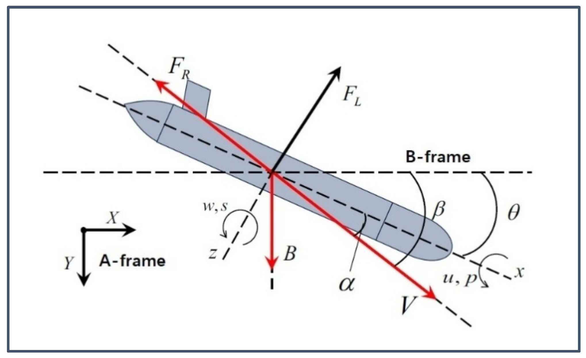
The proposed pre-compensation acts as a feed-forward layer that neutralizes steady-state current offsets. By providing the DMPC controller with this nonlinearly corrected nominal reference, the optimization burden is significantly reduced. This allows the rolling optimization and feedback correction stages of the DMPC to focus exclusively on dynamic disturbances and inter-agent coordination, thereby enhancing the robustness and convergence speed of the formation reconfiguration process in complex marine environments. We further discuss the operation rules under extreme conditions based on the system reachability. The reachability condition determines the executability of commands from the nonlinear heading pre-compensation. This pre-compensation works normally when the condition holds. When the reachability condition is violated, the nonlinear heading pre-compensation module is automatically disabled, and the system enters fallback mode. Since the underwater glider has no independent rudder, heading correction is achieved indirectly through pitch adjustment, which alters the glide angle and horizontal velocity vector.

Fallback control law: ${\theta }_{fb}=sat\left({\theta }_0+K_{\psi }\times \left({\psi }_d - \psi \right),0^{\circ },{35}^{\circ }\right)$, $K_{\psi }={15}^{\circ }/\mathrm{rad}$, ${\theta }_0=3^{\circ }$. Buoyancy is held at $\mathsf{\Delta }{B}_0=20$ mL. The RUI remains active (S = 1) during fallback because strong currents produce a high urgency index. While perfect tracking is impossible under these extreme conditions, the saturated pitch command ensures bounded deviation growth. Once reachability is restored, the DMPC command is smoothly reintroduced via Equation (43), in which the first term $u_{dormant}$ is replaced by $u_{fallback}$ during a fallback-to-DMPC transition.

4.2. Boundary-Triggering Mechanism

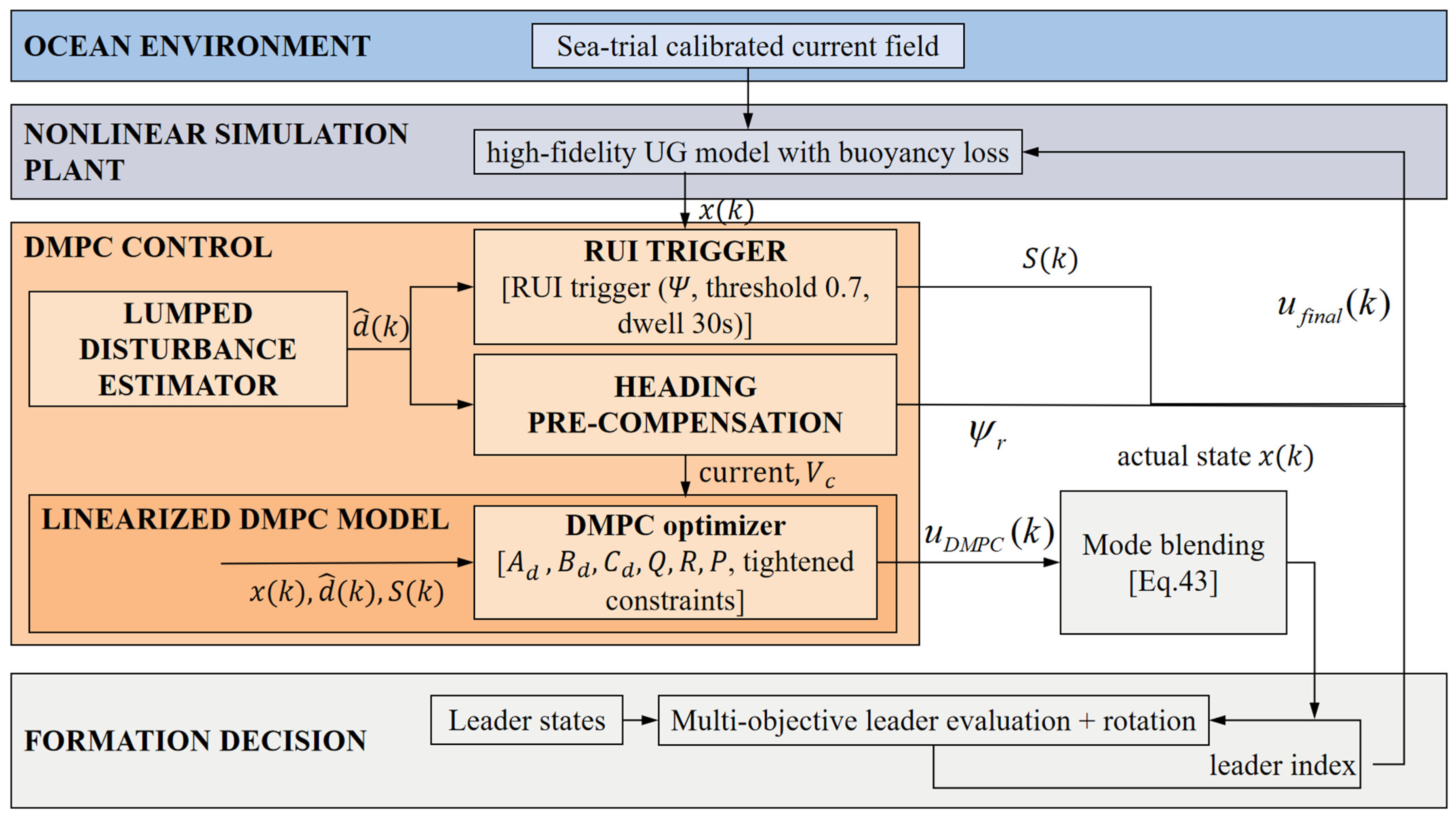
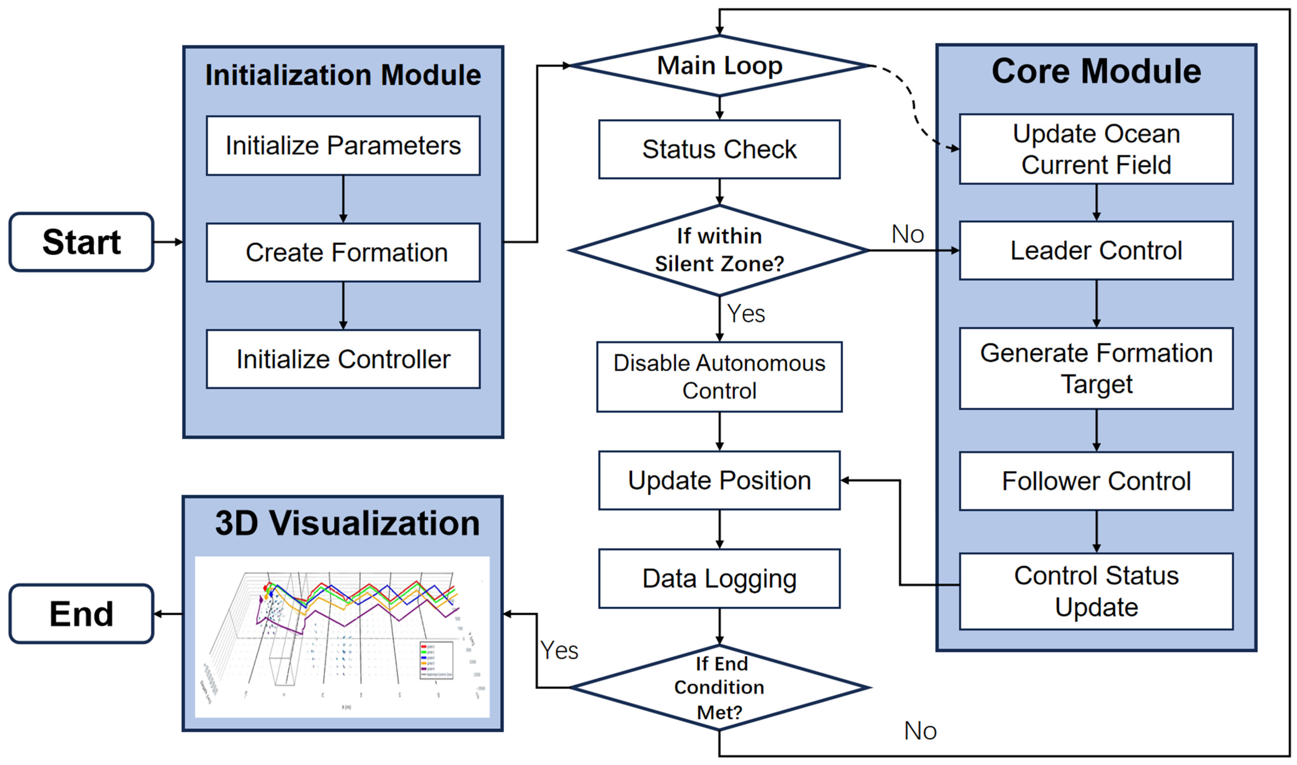
The overall control architecture of the proposed algorithm is illustrated in Figure 3, which distinguishes the nonlinear simulation plant, the linearized DMPC prediction model, and the lumped disturbance estimator. The process of UG formation operation and navigation of the silent zone is shown in Figure 4. When the UG descends to a specified depth within the silent zone, it activates the silent mode. In this mode, the glider maintains its current attitude and buoyancy to sustain a steady gliding state, with its detection equipment remaining operational. After proceeding to the preset navigation depth, it autonomously ascends to a designated depth. Subsequently, the silent mode is deactivated, and the glider autonomously adjusts its position to reconfigure the formation.

To balance energy efficiency in the silent zone and the precision of formation reconfiguration upon exit, a flexible triggering mechanism based on Reconfiguration Urgency Index (RUI) is proposed. This mechanism replaces static boundary switching with an environment-adaptive logic, ensuring that the DMPC controller can dynamically adjust its intensity based on the ocean current intensity and the deviation magnitude.

The transition from control suspension to active reconfiguration is no longer a simple binary switch. We define the RUI ($\mathsf{\Psi }$) as a function of the predicted formation tracking error and the estimated ocean current disturbance:

$$\mathsf{\Psi }(t)={\omega }_e{‖e_p(t)/e_{\max }‖}^2+{\omega }_v‖V_{curr}(t)/V_{\max }‖$$

(39)

where $e_p(t)$ is the predicted lateral deviation from the formation trajectory, $V_{curr}(t)$ is the real-time estimated ocean current speed, $e_{\max }=3000$ m is the maximum expected lateral deviation upon silent-zone exit (calibrated from sea trials), and $V_{max}=0.5$ m/s is the maximum expected current speed in the operational area. Both normalized terms ${‖e_p(t)/e_{\max }‖}^2$ and $V_{curr}(t)/V_{\max }$ are dimensionless and lie in [0,1]. The position-error term is squared to penalize large formation deviations nonlinearly—deviations beyond the nominal range trigger disproportionately stronger reconfiguration—while the current-velocity term is linear because ocean-current-induced drift is directly proportional to current speed. The sensitivity coefficients satisfy ${\omega }_e+{\omega }_v=1$ with ${\omega }_e, {\omega }_v\in \left[0,1\right]$.

The triggering state $S(t)$ is governed by

$$S(t)=\left\{\begin{array}{ll}0 \left(\mathrm{Dormancy}\right),\hfill & \mathrm{if} \mathsf{\Psi }(t)<{\mathsf{\Psi }}_{th}\hfill \\ 1 \left(\mathrm{Active}\right),\hfill & \mathrm{if} \mathsf{\Psi }(t)\ge {\mathsf{\Psi }}_{th}\hfill \end{array}\right.$$

(40)

where ${\mathsf{\Psi }}_{th}$ = 0.7 is a fixed threshold determined through grid search. To prevent repeated switching when $\mathsf{\Psi }\left(t\right)$ fluctuates near ${\mathsf{\Psi }}_{th}$, a dwell-time rule is enforced: after any state transition, the controller remains in the new state for at least $T_{dwell}=30$ s (3 sampling intervals), regardless of subsequent RUI values. The smooth sigmoid transition in Equation (43) further ensures that control commands remain continuous during mode changes. In a simulation, this rule eliminates spurious high-frequency switching while adding negligible latency to genuine reconfiguration triggers. The adaptivity to environmental conditions is provided by the time-varying weighting factor $\eta (t)$ described below. This RUI-based logic ensures that the UGs remain in a silent state when the environment is stable but can react instantaneously if strong currents cause critical deviations. The parameters were tuned via grid search over ${\omega }_e\in \left[0.3,0.8\right]$ (with ${\omega }_v=1-{\omega }_e$) and ${\mathsf{\Psi }}_{th}\in \left[0.4,0.9\right]$, using the integrated absolute lateral error over the reconfiguration phase as the tuning objective. The search used three recorded sea-trial current profiles covering weak (0.06–0.15 m/s), moderate (0.15–0.30 m/s), and strong (0.30–0.44 m/s) conditions.

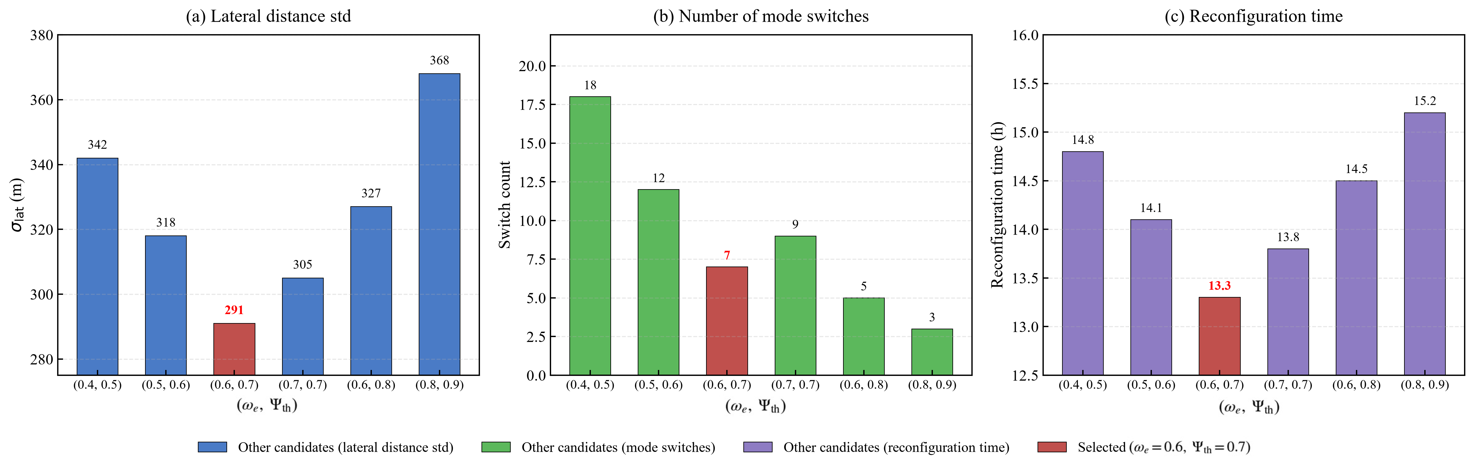
Figure 5 presents the RUI parameter sensitivity analysis. Among the six parameter combinations, the selected ${\omega }_e$ = 0.6, ${\omega }_v$ = 0.4, and ${\mathsf{\Psi }}_{th}$ = 0.7 achieve the lowest lateral distance standard deviation of 291 m and the shortest reconfiguration time of 13.3 h, with a moderate switch count of 7. Raising the threshold reduces switching but degrades tracking, whereas lowering it improves tracking at the cost of increased chattering.

First, a grid search is conducted over reasonable ranges of ${\omega }_e$, ${\omega }_v$ and ${\mathsf{\Psi }}_{th}$ to balance triggering responsiveness and anti-chattering performance, avoiding frequent state switching under mild disturbances.

Second, the optimal candidate parameters are calibrated using multiple sets of real sea trial data covering typical ocean current speeds in practical marine environments, ensuring adaptability to actual disturbance characteristics.

Finally, closed-loop stability verification is performed to guarantee reliable triggering logic under both weak and strong current conditions.

To address the theoretical depth regarding weight selection, we introduce an adaptive weighting law within the DMPC cost function. The penalty matrices’ state error $Q$ is dynamically scaled by the RUI to optimize the reconfiguration performance:

$$Q_{adj}(t)=\eta (t)\cdot Q_0$$

(41)

$$\eta \left(t\right)=1+\beta /\left[1+exp\left(-\left(\mathsf{\Psi }\left(t\right)-{\mathsf{\Psi }}_{th}\right)/\sigma \right)\right]$$

(42)

where $\eta (t)$ is the adaptive scaling factor, $Q_0$ is the baseline weight matrix, and $\beta$, $\sigma$ are shaping parameters. Specifically, $\beta =2.0$ denotes the maximum weight increment, $\sigma =0.15$ represents the transition width, and ${\mathsf{\Psi }}_{th}=0.7$ is the midpoint of the sigmoid transition. The sigmoid function is monotonically increasing, bounded in [1,3], and $C^{\infty }$-continuous. Under low disturbance, the weight returns to the baseline $Q_0$ as intended; under strong disturbance, it increases to prioritize rapid reconfiguration. This formulation implies that when the UG exits the silent zone or encounters strong current disturbances ($\mathsf{\Psi }(t)\ge {\mathsf{\Psi }}_{th}$), the weight on tracking error increases exponentially, forcing the DMPC to prioritize rapid reconfiguration. Conversely, in low-disturbance environments ($\mathsf{\Psi }(t)<{\mathsf{\Psi }}_{th}$), $\eta (t)$ approaches 1, maintaining the baseline state-error penalty $Q_0$. Energy savings under low disturbances are achieved primarily through the RUI keeping the controller in the dormant state, rather than through reducing the MPC weight below baseline.

While the RUI determines the timing of control activation, the transition of the actual control command $\mathit{u}(t)$ must respect the physical constraints of the UG’s actuators (e.g., the limited speed of the buoyancy engine and mass shifter). To prevent mechanical chattering or excessive structural stress caused by sudden control jumps, a continuous transition function $\sigma (\tau )$ is utilized:

$${\mathit{u}}_{final}(t)=\left[1-\sigma (\tau )\right]\cdot {\mathit{u}}_{dormant}+\sigma (\tau )\cdot {\mathit{u}}_{DMPC}(t)$$

(43)

where $\sigma (\tau )$ is a $C^1$-continuous mapping (such as a Sigmoid-based transition) over the transition interval $\tau$, and $u_{dormant}$ denotes the control command of the mode being exited; during a fallback-to-DMPC transition, this term is replaced by $u_{fallback}$.

4.3. Multi-Objective Leader Capability Evaluation and Rotation Strategy

In an environment with ocean current disturbances, after the UG formation traverses the silent zone, it needs to achieve smooth switching of control states and dynamic rotation of the leader vehicle. This strategy is an intelligent control mechanism inspired by nature, whose core idea originates from the lead goose rotation behavior in long-distance flight of goose flocks, ensuring the group completes long-distance migration with optimal efficiency through balanced energy distribution [29]. This study applies this bionic principle to UG formation control, integrating three optimization objectives—energy, position, and communication—to establish a dynamic leader-switching mechanism based on multi-objective leader capability evaluation.

First, candidate set screening selects an eligible candidate leader glider from all UGs, mathematically defined as

$${\mathsf{\Omega }}_{candidate}=\{i\in \mathcal{N}\mid E_i\ge E_{th}, P_{match,i}\ge P_{th}\}$$

(44)

where $E_i$ is the remaining energy state indicator of glider $i$, and $P_{match,i}$ is its position-matching degree. $E_{th}$ is the energy threshold, ensuring the candidate leader has sufficient energy to complete the scheduling task; $P_{th}$ is the position-matching degree threshold, requiring the candidate glider to be located in the core area of the formation.

The position-matching degree $P_{match,i}$ is calculated using a Gaussian function:

$$P_{match,i}=\exp \left(-{\displaystyle \frac{\left|\right|p_i-p_{center}|{|}^2}{2{\sigma }_p^2}}\right)$$

(45)

where ${\sigma }_p$ is the formation position tolerance radius, selected via grid search over [300, 800] m. A larger ${\sigma }_p$ admits more candidate leaders; a smaller ${\sigma }_p$ restricts candidates to the formation core.

Second, the optimal leader glider is determined from the candidate set. The decision formula is

$$i^{*}=\arg \underset{i\in {\mathsf{\Omega }}_{candidate}}{\max }{J}_{eval}(i)$$

(46)

A comprehensive evaluation function is constructed as follows:

$$J_{eval}(i)=w_1{\overline{E}}_i+w_2{\overline{P}}_{match,i}+w_3{\overline{C}}_{comm,i}$$

(47)

where ${\overline{E}}_i$ is the normalized energy state indicator, ${\overline{P}}_{match,i}$ is the normalized position state indicator, and ${\overline{C}}_{comm,i}$ is the normalized communication quality indicator. $w_1,w_2,w_3$ correspond to the weighting coefficients for the energy, position, and communication indicators, respectively, and $w_1+w_2+w_3=1$. The grid-search ranges are $w_1\in \left[0.2,0.6\right]$, $w_2\in \left[0.2,0.5\right]$, $w_3\in \left[0.1,0.4\right]$, $E_{th}\in \left[20\%,50\%\right]$, $P_{th}\in \left[0.4,0.8\right]$, and ${\sigma }_p\in \left[300,800\right]$ m. The selected values are $w_1$ = 0.4, $w_2$ = 0.35, $w_3$ = 0.25, $E_{th}$ = 30% and $P_{th}$ = 0.6.

Finally, the leader authority switching is performed using an exponential decay-based formula as follows:

$${\mathit{u}}_{new}=e^{-k(t-t_0)}{\mathit{u}}_{current}+[1-e^{-k(t-t_0)}]{\mathit{u}}_{t\arg et}$$

(48)

where $t_0$ is the switching initiation time; k is the convergence rate parameter (optimized to k = 0.15 s⁻¹); and ${\mathit{u}}_{current}$ and ${\mathit{u}}_{t\arg et}$ are the control quantities of the current leader and target leader.

To prove the stability of the above equation, define the control error $e={\mathit{u}}_{\mathrm{new}}-{\mathit{u}}_{\mathrm{ideal}}$, whose dynamic equation is

$$\dot{e}=-ke+d(t)$$

(49)

where $d(t)$ is a bounded disturbance. Choosing the Lyapunov function $V(e)={\displaystyle \frac{1}{2}}{e}^{T}e$, its derivative is as follows:

$$\dot{V}=e^T\dot{e}=-k\parallel e{\parallel }^2+e^{T}d(t)\le -k\parallel e{\parallel }^2+\parallel e\parallel \parallel d\parallel$$

(50)

When $\parallel e\parallel >\parallel d\parallel /k$, we have $\dot{V}<0$. Therefore, for any $k>0$ and bounded $\parallel d\parallel$, the control error e is uniformly ultimately bounded (UUB), converging to the residual set $\parallel e\parallel \le \parallel d\parallel /k$. The selected convergence rate $k=0.15 s^{-1}$ satisfies $k>0$ and, thus, guarantees UUB stability.

4.4. Closed-Loop Stability Analysis of the Hybrid System

The hybrid system follows the ZOH discrete model from Section 3.1:

$$x(k+1)=A_{d}x(k)+B_{d}u(k), y(k)=C_{d}x(k)$$

where $d(k)$ in $\mathcal{W}$ is the bounded lumped disturbance, $\mathcal{W}$ is derived from the Section 3.4 disturbance observer; $\mathcal{Z}$ is the RPI set satisfying $A_d\mathcal{Z}\oplus \mathcal{W}\subseteq \mathcal{Z}$; tightened constraints $\overline{\mathit{x}}\in \mathcal{X}\ominus \mathcal{Z},v\in \mathcal{U}\ominus \mathit{K}\mathcal{Z}$; and the terminal invariant set ${\mathcal{X}}_f$ satisfies $A_d{\mathcal{X}}_f\oplus B_d\mathcal{U}\subseteq {\mathcal{X}}_f$. The adaptive weights satisfy ${\mathbf{Q}}_{\mathbf{m}\mathbf{i}\mathbf{n}}\le \mathit{Q}(\mathsf{\Psi }(k))\le {\mathbf{Q}}_{\mathbf{m}\mathbf{a}\mathbf{x}},{\mathbf{R}}_{\mathbf{m}\mathbf{i}\mathbf{n}}\le \mathit{R}(\mathsf{\Psi }(k))\le {\mathbf{R}}_{\mathbf{m}\mathbf{a}\mathbf{x}}$.

Theorem 1.

Under bounded ocean disturbances, the discrete DMPC formation system satisfies the following:

a.

Recursive feasibility: Feasible control sequences exist for all $k+1,k+2,\dots$ if feasible at instant $k$;

b.

DUUB stability: All closed-loop states converge to a compact invariant set ${\mathsf{\Omega }}_{\mathrm{UUB}}.$

Proof of Recursive Feasibility.

Suppose that at time $k$, the optimal nominal sequence ${\{\overline{x}(k+i|k),v(k+i|k)\}}_{i=0}^{N_p}$ meets tightened constraints and $\overline{x}(k+N_p|k)\in {\mathcal{X}}_f$.

The candidate sequence for $k+1$ is constructed:

$$\left\{\begin{array}{c}\overline{\mathit{x}}(k+1+i|k+1)=\overline{\mathit{x}}(k+1+i|k),i=0,\dots ,N_p-1\\ \mathit{v}(k+1+i|k+1)=\mathit{v}(k+1+i|k),i=0,\dots ,N_p-2\\ \mathit{v}(k+N_p|k+1)=0\end{array}\right.$$

(51)

Terminal condition: $(\overline{\mathit{x}}(k+N_p|k+1)=A_d\overline{\mathit{x}}(k+N_p|k)+B_d\mathit{v}(k+N_p|k)\in {\mathcal{X}}_f$. All tightened constraints hold. By induction, recursive feasibility holds for all discrete steps. □

Proof of DUUB Stability.

Take the discrete Lyapunov function as the optimal cost $V(k)=J^{*}(\overline{\mathit{x}}(k),\mathsf{\Psi }(k)$, with the following cost function:

$$J={\displaystyle {\displaystyle \sum _{\tau =1}^{N_p}}{‖{\mathit{y}}_{\mathit{p}}-{\mathit{y}}_{\mathit{r}}‖}_{\mathit{Q}(\mathsf{\Psi })}^2}+{\displaystyle {\displaystyle \sum _{\tau =0}^{N_p-1}}{‖\mathsf{\Delta }v‖}_{\mathit{R}(\mathsf{\Psi })}^2}+{‖\overline{\mathit{x}}(k+N_p)‖}_P^2$$

(52)

Lyapunov difference:

$$\begin{array}{l}\mathsf{\Delta }V(k)=V(\overline{\mathit{x}}(k+1),\mathsf{\Psi }(k+1))-V(\overline{\mathit{x}}(k),\mathsf{\Psi }(k))=T_1+T_2\\ T_1=V(\overline{\mathit{x}}(k+1),\mathsf{\Psi }(k))-V(\overline{\mathit{x}}(k))\\ T_2=V(\overline{\mathit{x}}(k+1),\mathsf{\Psi }(k+1))-V(\overline{\mathit{x}}(k+1),\mathsf{\Psi }(k))\end{array}$$

(53)

• Nominal descent term: $T_1\le -{‖\overline{e}(k)‖}_{Q_{\min }}^2-{‖\mathsf{\Delta }v(k)‖}_{R_{\min }}^2+{\sigma }_{\mathrm{dist}}$. ${\sigma }_{\mathrm{dist}}$ is a fixed upper bound of the disturbance cost increment.
• Weight-switching term: $\mathsf{\Psi }(k)$ is Lipschitz-continuous, so $\left|T_2\right|\le L_w|\mathsf{\Psi }(k+1)-\mathsf{\Psi }(k)|$.

$\mathsf{\Delta }V(k)\le -{‖\overline{e}(k)‖}_{Q_{\min }}^2-{‖\mathsf{\Delta }v(k)‖}_{R_{\min }}^2+{\sigma }_{\mathrm{dist}}+L_w\left|\mathsf{\Delta }\mathsf{\Psi }(k)\right|$ is combined. ${\mathsf{\Omega }}_{\mathrm{UUB}}=\{\overline{x}\mid -\Vert \overline{e}{\Vert }_{Q_{\min }}^2+{\sigma }_{\mathrm{dist}}+L_w\sup |\mathsf{\Delta }\mathsf{\Psi }|\ge 0\}$ is defined. For $\overline{x}(k)\notin {\mathsf{\Omega }}_{\mathrm{UUB}}, \mathsf{\Delta }V(k)<0$, so states stay bounded inside ${\mathsf{\Omega }}_{\mathrm{UUB}}$. □

• Dynamic Leader Switch Supplementary

The switching law $u_{new}(k)= {\alpha }^{k-k0}{u}_{current}+(1-{\alpha }^{k-k0})u_{target}$, with $\alpha =e^{-k{T}_s}=e^{-1.5}\approx 0.223$ for $k=0.15s^{-1}$ and $T_s= 10 s$, yields discrete error dynamics $e_u\left(k+1\right)=\alpha e_u\left(k\right)+d_s\left(k\right)$. Since $\left|\alpha \right|=0.223<1$, the error system is Schur-stable. The bounded switching perturbation $d_s(k)$ is absorbed into ${\sigma }_{dist}$ without breaking DUUB. No separate $k_s$ parameter is used.

The ZOH discrete DMPC formation system is recursively feasible and DUUB-stable under time-varying ocean disturbances. All theoretical derivations match Section 3.1’s discrete model and support the simulation results in Section 5.

5. Simulation Results and Discussions

All numerical simulations in this study were independently implemented in Python 3.11, where the high-fidelity underwater glider dynamics, realistic ocean current environment, and seabed terrain model were self-developed and calibrated using real sea trial data. We conducted comparative simulations to verify the effectiveness of the proposed algorithm for formation reconfiguration under ocean current disturbances; a formation simulation involving five UGs was conducted. First, a simulation environment with a complex flow field was established; secondly, following the algorithm procedure, a formation reconfiguration simulation based on the DMPC algorithm was carried out, and the motion characteristics were analyzed; and finally, a comparative simulation of formation control was conducted with the ADRC and conventional MPC algorithms. All controller comparisons in this study were conducted in numerical simulations. The sea-trial data were used solely for (i) calibrating the high-fidelity nonlinear plant model and (ii) generating realistic current profiles.

To ensure the rigor and fairness of the comparative study, all simulations were conducted within a unified computing environment and under identical environmental constraints.

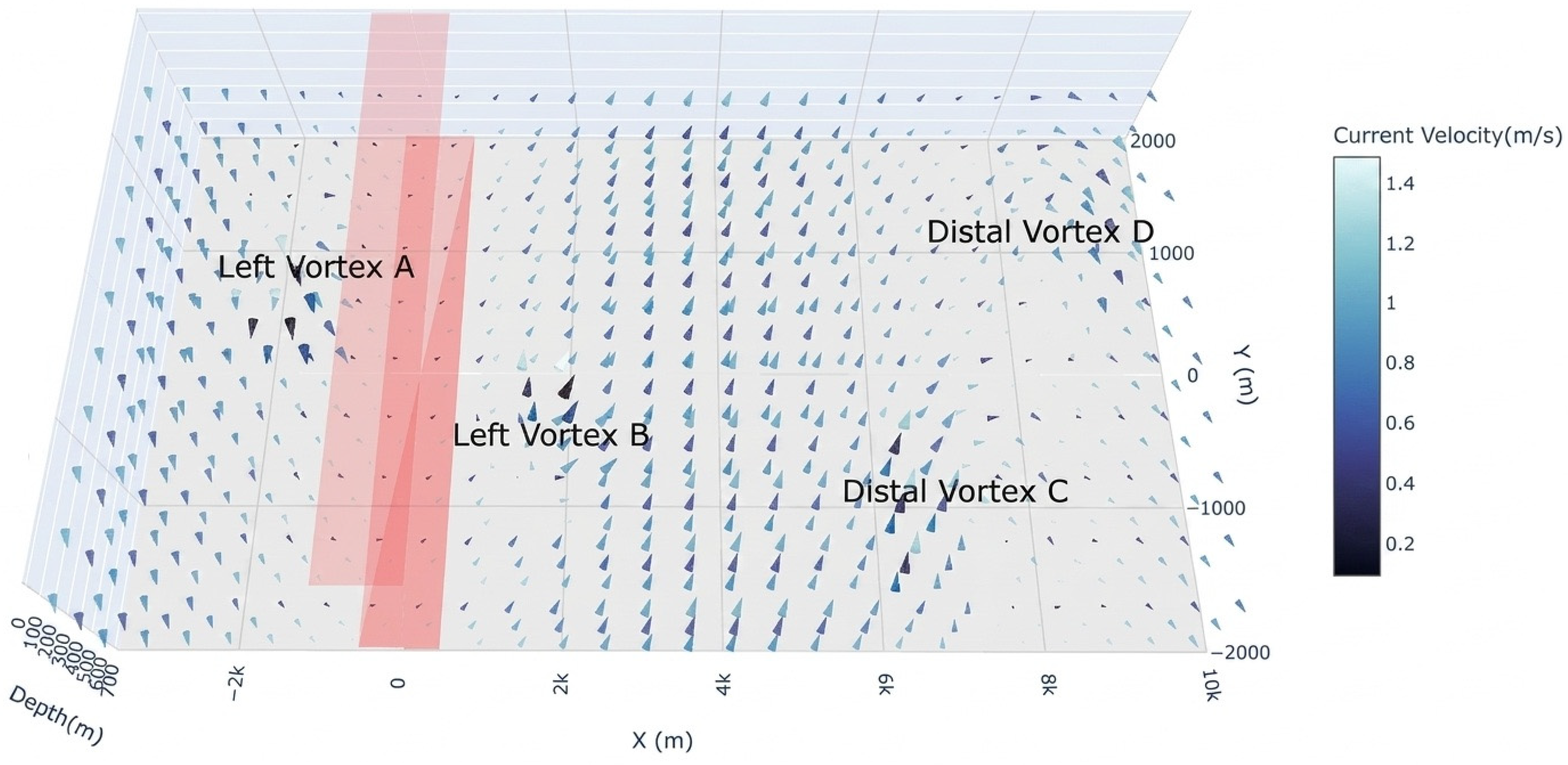
The simulation area was set with an X-axis range from −3500 to +10,000 m and a Y-axis range from −2000 to 2000 m. A silent zone was established within the $x\in \left[-500,500\right]$ meter area, and multiple vortex regions were set, as shown in Figure 6 below.

The core performance of MPC lies in whether its predictive model can accurately foresee the system’s behavior over a future time horizon. Traditional predictive models are mostly trained in idealized static environments [30]. To enhance the model’s predictive capability in complex, time-varying ocean current environments, this paper considers the impact of the marine environment on UG performance. Ocean current data synchronously collected during sea trials were used as a crucial environmental input, training the improved predictive model alongside the UG’s control inputs. The improved model can more accurately predict the forces and motion trends of a UG in a specific current field, thereby enabling the DMPC controller to “foresee” the deviation caused by currents and generate optimized control commands with compensatory effects in advance.

The performance verification of the proposed formation reconfiguration algorithm was implemented based on high-fidelity numerical simulation. To avoid simulation deviation caused by idealized dynamic models and ensure the simulation results had sufficient engineering reference value, real sea trial data of the UG were adopted to complete accurate hydrodynamic parameter identification and high-fidelity calibration of the glider dynamic model. The calibrated model can accurately characterize the actual motion characteristics of the UG in real marine environments, building a solid and reliable physical foundation for the numerical simulation of multi-glider formation control and reconfiguration.

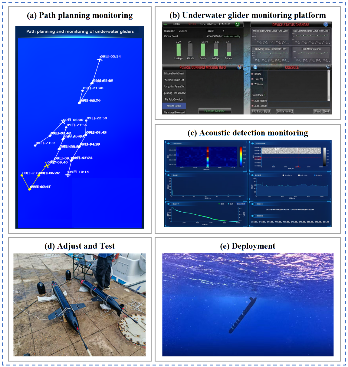
This paper extracted and analyzed UG operational data from the sea trial period. Details of the sea trial are shown in Figure 7. Among them, (a) is the UG formation path-planning monitoring platform, which can intuitively monitor the location and time information of the UG’s water entry/exit points transmitted to the shore-based platform; (b) is the UG control platform; (c) is the UG acoustic detection platform, which can visually display detection results; (d) shows the UG debugging scenario; and (e) shows the entry of the UG into the water. The technical parameters of the UG are shown in

Table 2. Technical specifications.

Parameter	Value	Parameter	Value/Type
Fuselage length (m)	1.7	Main-body diameter (cm)	22
Weight in air (kg)	≈83	Power source type	Lithium battery
Maximum operating depth (m)	1200	Communication/positioning	Wireless/BeiDou
Designed endurance (days)	≥90	Sensor configuration	CTD/hydrophone

. Based on the data collected from sea trials and the UG’s technical parameters, the UG dynamic model was optimized. The focus was on identifying the hydrodynamic parameters $K_R$ and $K_L$. Using the least squares method to fit 13 sets of sea trial data, the optimal solutions for the key hydrodynamic parameters of the UG were obtained through optimization calculations: drag coefficient $K_R$ = 0.042; lift coefficient $K_L$ = 0.087. Furthermore, the effect of ocean currents on the UG’s motion was analyzed to determine a sea-trial-calibrated compensation coefficient. Processing the 13 datasets, which covered current speeds from 0.06 m/s to 0.44 m/s, resulted in an optimal calibrated compensation coefficient of $k_c$ = 0.623. The parameter identification and optimized dynamic model provide a more accurate predictive foundation for DMPC.

The proposed algorithm adopts a DMPC framework, as illustrated in Figure 4. Its core procedure comprises three stages:

• Initialization Layer: Create the formation structure (initialize UG positions and dynamic parameters) and construct the controller (DMPC weights and constraint boundaries), while synchronously loading the ocean current field model and the coordinates of the silent zone.
• State Detection Layer: In the main loop, the formation position is monitored in real-time via a flexible boundary-triggering mechanism. Within the silent zone, the system is forced to switch to a no-autonomous-control mode; after exiting the zone, the controller is activated to guide reconfiguration.
• Cooperative Decision-Making Layer: The ocean current model is updated through flow field prediction. Based on a multi-objective leader capability evaluation mechanism, the dynamic switching between the leader and followers is determined, and formation objectives are generated in a distributed manner.

For a fair comparison, all three controllers share identical actuator constraints, identical initial conditions, identical sea-trial-derived current profiles, and the same energy consumption model. The MPC and ADRC parameters were tuned via grid search, using the minimum standard deviation of lateral inter-glider distance as the objective criterion. The standard deviation of lateral inter-glider distance is computed as follows: during the reconfiguration phase, the lateral distance between each follower and the leader is recorded at every sampling instant. For each follower, the temporal standard deviation of this lateral distance is computed; the reported metric is then the mean of these standard deviations over all four followers. The search ranges are MPC: state weights searched over $\{diag=\left(1,1,1\right), diag=\left(5,5,5\right)$$, diag=\left(10,10,5\right), diag=\left(12,12,6\right)\}$, from which $diag=\left(10,10,5\right)$ was selected for conventional MPC and $diag\left(12,12,6\right)$ for the proposed DMPC. All candidates are three-dimensional, consistent with $y={[x,y,\psi ]}^T\in R^3$, control weights over $\left\{diag\left(0.01,0.01\right), diag\left(0.1,0.1\right), diag\left(1,1\right)\right\}$, and a prediction horizon over $\left\{10, 15, 20\right\}$. ADRC: TD speed factor searched over $\left[50, 200\right]$, ESO gains over typical ranges (${\beta }_1\in \left[100, 500\right],{\beta }_2\in \left[300, 1000\right],{\beta }_3\in \left[500, 2000\right]$), NLSEF gain in $\left[0.5, 2.0\right]$, and compensation factor in $\left[0.5, 1.5\right]$. All tuning and comparative evaluations were conducted in simulation only, using the data-driven plant model and sea-trial-calibrated current profiles. The sea trial data served solely for model calibration and current-profile generation. Detailed constraints and key parameter configurations for the traditional MPC, DMPC and ADRC are provided in Table 1 and

Table 3. Parameters for ADRC.

Module	Parameters	Value	Description
Tracking Differentiator (TD)	Speed factor/$r_0$	100	Determines the tracking speed of the differentiator
	Filter factor/$h_0$	0.01	Suppresses noise and smooths input signals
Extended State Observer (ESO)	Observer gain 1/${\beta }_1$	200	Adjusts the tracking speed of the system state
	Observer gain 2/${\beta }_2$	500	Adjusts the estimation accuracy of the system state
	Observer gain 3/${\beta }_3$	1000	Adjusts the estimation accuracy of the total disturbance
Nonlinear State Error Feedback (NLSEF)	Nonlinear factor/$\delta$	0.5	Determines the nonlinearity of the feedback law
	Control gain/$b_0$	1.2	Adjusts the magnitude of the control output
Compensation Module	Disturbance compensation factor/$c$	0.9	Compensates for the residual disturbance in the system

. All controllers are evaluated under strictly identical conditions to ensure a fair comparison. Uniform actuator limits apply a consistent pitch angle range and buoyancy adjustment constraints across all controllers. Consistent energy assumptions use the same initial battery level and real-data-based energy consumption model for all cases. Identical environmental disturbances adopt the same measured ocean current profiles and disturbance models in all simulations and sea trials, eliminating external condition bias.

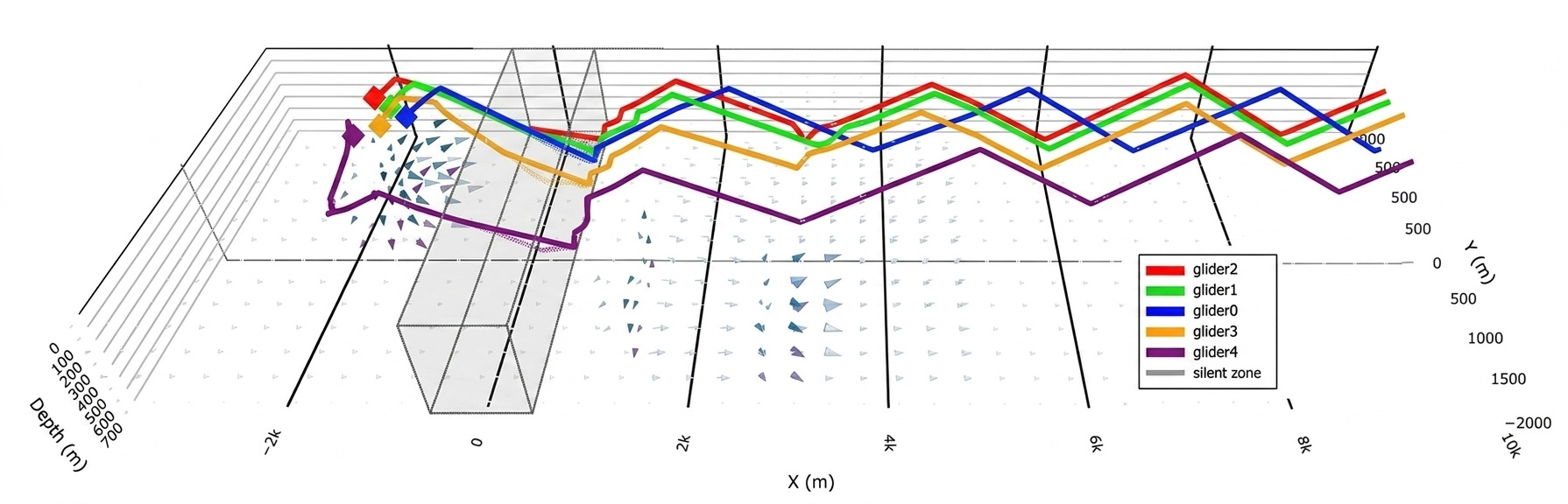
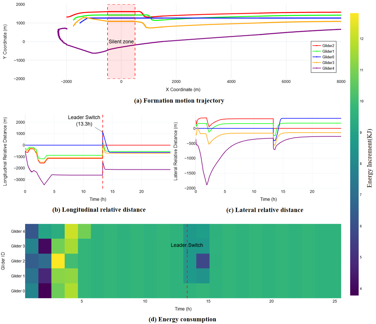
Running the simulation code yielded the three-dimensional trajectory of the UG formation reconfiguration in the core area, as shown in Figure 8. As evidenced by the trajectories, ocean currents caused substantial disruption to the gliders. Notably, Glider 4 experiences significant passive drift away from the intended formation path prior to entering the silent zone. The formation enters the silent zone, where the non-autonomous control mode is activated, and each UG passes through the silent zone solely under the influence of ocean currents. After reaching the exit boundary of the silent zone, the flexible boundary activation mechanism is triggered, initiating autonomous adjustments of the motion attitude to ascend to the surface in the shortest possible time and restore formation communication. Integrating the first surfacing point communication information from each UG, the leader switch is executed based on the multi-objective leadership evaluation mechanism and dynamic switching strategy, completing the transition from Glider 0 to Glider 2 as the leader after 13.3 h of operation.

To analyze the impact of DMPC on formation reconfiguration in detail, operational data were retrieved and plotted, resulting in the formation motion characteristic curves shown in Figure 8 below.

Figure 9a shows the motion trajectory of the UG formation under ocean current disturbance, displaying the formation’s travel route during the silent-zone navigation. The UG formation, after traversing the silent zone, can quickly converge towards the preset formation structure, effectively coping with ocean current disturbances.

Figure 9b presents the variation curve of the longitudinal relative distance within the formation. The longitudinal relative distance refers to the distance difference in the forward direction between the follower gliders and the leader glider in the formation. Before entering the silent zone, influenced by currents from different directions, Glider 4 separates from the formation, with a maximum longitudinal distance difference from the leader exceeding 3500 m; after exiting the silent zone, Glider 4 quickly activates and adjusts its attitude to catch up with the formation, forming the formation structure after 13.3 h of total operation.

Figure 9c displays the lateral relative distance variation graph, and Figure 9d displays the energy consumption chart for each UG, revealing the dynamic behavior and energy consumption characteristics of the UG formation during the mission cycle. By combining the two figures, it can be seen that from 0 to 2 h, within the silent zone, all gliders are in a low-energy-consumption state; after exiting the silent zone, each glider begins to execute formation reconfiguration. Among them, Glider 4 has relatively high energy consumption, experiencing significant deviation due to ocean current influence; concurrently, the average energy consumption graph in Figure 9d shows that this UG had a higher average energy consumption during the 0~6 h period, a phenomenon reflecting the high energy consumption characteristic of its prolonged attitude correction. Integrating and adjusting data such as the energy consumption status and relative positions of each glider, and conducting a quantitative evaluation through the multi-objective leadership assessment mechanism, can provide decision-level support oriented towards energy consumption optimization for the dynamic role switching in UG formations.

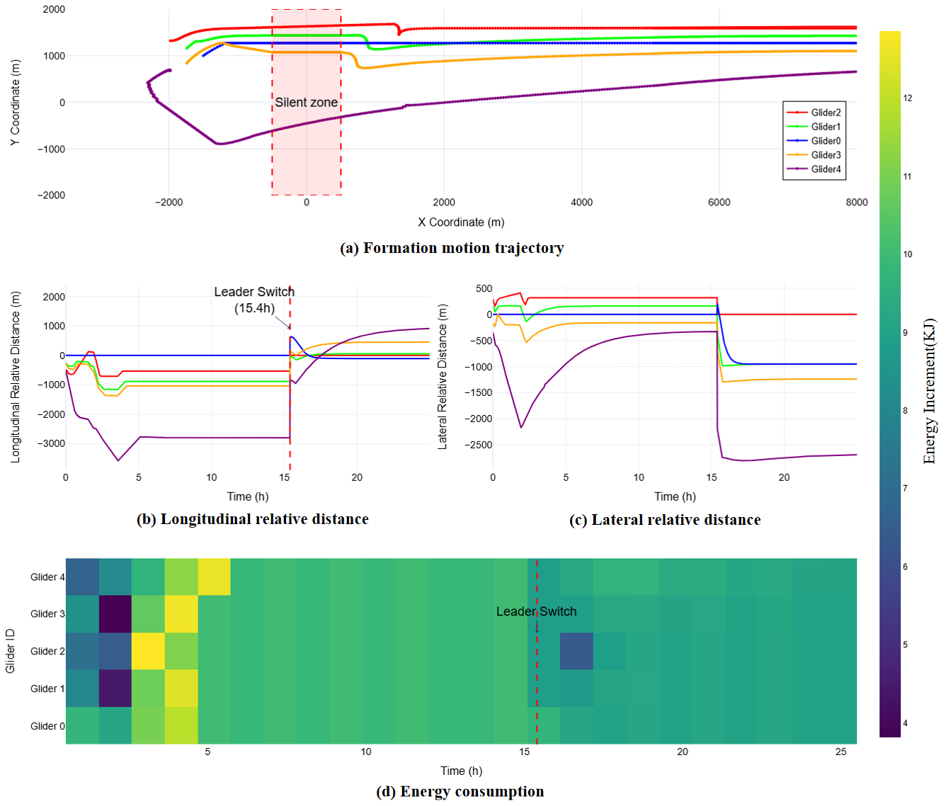
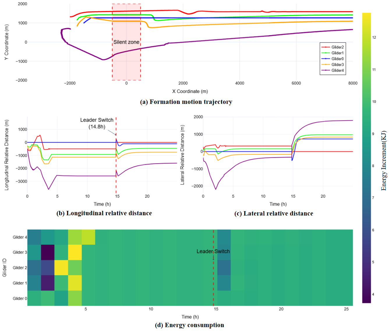
To quantitatively evaluate the practical effectiveness of the advanced control algorithm in underwater cooperative operations, this paper conducts a comparative experiment between the proposed algorithm and the widely used ADRC-based as well as conventional MPC in current UG applications. Through quantitative analysis of the formation motion characteristics in Figure 9, Figure 10 and Figure 11, a comparison of key metrics is presented, as shown in

Table 4. Comparison of key indicators.

Indicators	DMPC	MPC	ADRC
Reconfiguration time/h	13.3	14.8	15.4
Maximum relative deflection/m	1934	2230	2754
Standard deviation of lateral distance/m	291	352	502
Average energy/kJ	121.8	122.9	122.4

.

Regarding formation keeping and cooperative accuracy, by comparing subfigures (a) and (c) of Figure 9, Figure 10 and Figure 11, it is observed that the ADRC-controlled Glider 4 exhibits the largest lateral offset. In contrast, DMPC, through distributed cooperative optimization, results in more convergent formation trajectories, with the maximum offset of Glider 4 being reduced by approximately 250 m compared with ADRC. Furthermore, after the leader switch stabilizes, data combined from the figures and tables indicate that under DMPC, the standard deviation of inter-glider distances is 291.23 m, which is 42% and 17% lower than that under ADRC and conventional MPC, respectively. This demonstrates a more uniform lateral distribution of the UGs under DMPC. Comparing the longitudinal distances in subfigure (b) of Figure 9, Figure 10 and Figure 11, during the silent-zone navigation, Glider 2 in the ADRC-controlled UG formation overtakes the leader around the 2 h mark, a situation that also occurs under conventional MPC. This indicates that the latter two exhibit weaker resistance to current disturbances compared with the DMPC-controlled formation. Furthermore, they struggle to maintain the correct “master–slave” longitudinal relative position after the leader switch event. In contrast, under DMPC, the longitudinal relative positions of the gliders are more stable, although Glider 4 also experiences a large longitudinal relative distance due to current influence. This phenomenon reflects the challenge of underwater gliders as underactuated systems having weak resistance to currents in real environments [31].

The advantage of DMPC is also evident in terms of energy consumption optimization. Analysis of the average energy consumption graph in Figure 9d reveals distinct phased characteristics in the energy consumption of each UG during the 25 h navigation. In the initial phase of 0–5 h, the energy consumption of each UG is relatively balanced, averaging about 4.5–5 kJ per hour. During the 5–10 h period after entering the silent zone, the consumption decreases to the range of 2.5–3 kJ, representing a significant reduction of 40–50% compared with the ADRC strategy. A significant fluctuation occurs at the leader switch time (13.3 h): the new leader Glider 2 experiences an instantaneous 20% increase in energy consumption to 5.5–6 kJ, while that of the original leader Glider 0 decreases by 25% to 2.5–3 kJ. During the subsequent formation reconfiguration period (14–18 h), the energy consumption of all UGs temporarily increases by 10–15%, finally stabilizing at an average of 4–4.5 kJ per hour from 18 to 25 h. Combined with Table 4, it is evident that under DMPC, the average energy consumption per vehicle for the 25 h navigation is 121.8 kJ, which is lower than the 122.4 kJ under ADRC and the 122.9 kJ under conventional MPC. DMPC demonstrates more efficient energy consumption control at event points such as leader authority switching and entering/exiting the silent zone. This research aims to reveal the core differences between the three control methods in maintaining multi-glider cooperative motion in complex marine environments. The results demonstrate that DMPC holds significant advantages over ADRC and conventional MPC in key performance metrics such as formation convergence, motion synchrony, and energy efficiency. Note that although the proposed DMPC achieves the lowest average energy consumption, the numerical difference from conventional MPC and ADRC is relatively small. However, this improvement carries important practical value for long-duration underwater glider operations. First, given the modest energy savings (0.5–0.9%), the endurance benefit should be regarded as potential rather than conclusively demonstrated in this study. Over multi-month missions, even small per-cycle savings could accumulate, but a rigorous endurance quantification would require long-duration simulations or field trials, which are left for future work. Second, the algorithm’s adaptive energy regulation reduces unnecessary control actuation during silent-zone navigation, which is critical for maintaining low-power operation and covertness. Third, the balanced energy distribution via dynamic leader rotation avoids localized energy depletion, ensuring sustained formation stability and reliable cooperative performance under complex ocean current disturbances.

6. Conclusions

This study addresses the issues of trajectory deviation in underwater glider (UG) formations caused by ocean current disturbances and rapid reconfiguration after traversing silent zones. A cooperative algorithm based on DMPC is proposed, which integrates a flexible boundary-triggering mechanism and a dynamic rotation strategy featuring multi-objective leader capability evaluation. The following main conclusions are drawn based on validation through simulation experiments and real sea trial data.

First, regarding formation-keeping performance, the proposed algorithm reduces the influence of ocean current disturbances on the formation trajectory through a heading pre-compensation model and the rolling optimization control of DMPC. The simulation results indicate that the standard deviation of the lateral inter-glider distance is reduced by 42% and 17% compared with traditional ADRC and MPC, respectively, thereby enhancing the formation’s stability during ocean observation missions.

Second, in terms of reconfiguration efficiency, the flexible boundary-triggering mechanism enables the suspension of autonomous control within the silent zone and its rapid reactivation after exit. Combined with the multi-objective leader capability evaluation and dynamic rotation strategy, the formation recovery time is reduced to 13.3 h.

Third, concerning energy consumption optimization, the dynamic leader rotation strategy balances the energy distribution across the formation. This yields a lower average energy consumption than the other two strategies, verifying the algorithm’s adaptability to complex marine environments and its energy efficiency, thereby providing a theoretical foundation for subsequent long-duration formation navigation trials.

The proposed multi-glider formation reconfiguration strategy is validated primarily through numerical simulations calibrated with sea trial data. While the simulations are based on high-fidelity models calibrated with sea-trial data, there remain potential discrepancies between simulation results and real-world underwater glider operations. Therefore, future work will focus on conducting comprehensive experimental validation, including field sea trials and hardware-in-the-loop tests, to further verify the practical performance and robustness of the proposed strategy in real marine environments.