Ship Docking Motion Prediction and Collision-Risk Early Warning Using a Physics–SVR Model

Abstract

Reliable collision-risk warning during low-speed ship docking requires accurate and efficient hydrodynamic prediction. This study develops a physics-SVR (support vector regression) framework combining a three-degree-of-freedom maneuvering model with three SVR models that learn residuals in longitudinal force, lateral force, and yaw moment from computational fluid dynamics (CFD) data. The corrected loads support 120 s trajectory prediction and hull-envelope reconstruction. Minimum lateral and longitudinal clearances and their times to safety-threshold crossing distinguish normal, warning-alert, and emergency-alarm states. The database comprises 20 model-development conditions and three condition-level holdout tests representing unseen loading/draft, heading, and lateral-offset conditions. Across the holdout tests, overall relative errors decrease from 22.00–30.20% for the baseline model to 14.91–19.93%. In two hazardous cases, warning alerts precede contact by 154.9 and 172.09 s, while the non-hazardous control case triggers no alarm. The complete prediction-and-warning update requires 0.32 s on average, demonstrating potential for shore-based docking assistance under calm-water conditions.

1. Introduction

Ship docking is a critical operation in ship repair, maintenance, and construction, during which large vessels are maneuvered at low speeds into confined dock chambers with limited clearance from the dock walls and end structures [1,2,3,4]. In this study, docking refers specifically to the low-speed entry of a ship into a dry-dock chamber rather than conventional berthing alongside a quay. Compared with open-water navigation, ship motion during docking is more strongly affected by shallow water, blockage, and hull–boundary interactions. Even small deviations in ship position or heading may lead to contact with the surrounding structures, causing structural damage, operational delays, and economic losses. Accurate short-term motion prediction and timely collision-risk warning are therefore essential for improving the safety of ship docking operations.

Automatic berthing and docking have been extensively investigated as important components of autonomous ship operation. Early studies generally formulated berthing as a nonlinear control or optimal maneuvering problem and determined the rudder, propeller, and thruster commands required to reach a prescribed terminal position and heading. Artificial neural networks were subsequently introduced to approximate nonlinear berthing control laws and improve real-time implementation [5,6,7]. Recent reviews have shown that automatic berthing research has progressively expanded to path planning, path following, direct optimal control, model predictive control, supervised learning, reinforcement learning, and collision-free trajectory generation [8,9,10,11,12,13,14,15,16]. These methods have considerably improved trajectory tracking, disturbance rejection, terminal-state accuracy, and control adaptability. However, their primary objective is generally to determine how a ship should be controlled to reach a target berth, while the underlying ship-motion model is commonly treated as a known or previously identified component. The accuracy of hydrodynamic-force prediction in highly confined dock chambers has received comparatively less attention.

Accurate prediction of low-speed ship motion is a prerequisite for both automatic docking control and collision-risk assessment. Classical ship maneuvering models include the Nomoto, Abkowitz, and MMG formulations [17,18,19,20]. Among them, the MMG model has been widely adopted because it provides a physically interpretable and modular representation of the forces generated by the hull, propeller, and rudder. Empirical hydrodynamic derivatives and maneuverability prediction methods have also been developed for general, shallow-water, and restricted-water conditions [21,22,23,24]. These physics-based models are computationally efficient and suitable for real-time simulation. Nevertheless, their hydrodynamic coefficients are commonly derived from empirical formulas, captive model tests, or regression relationships. Their prediction accuracy may deteriorate inside dock chambers, where shallow-water effects, dock–wall interaction, and blockage occur simultaneously and produce strongly coupled nonlinear hydrodynamic forces.

High-fidelity computational fluid dynamics provide an effective approach for resolving nonlinear ship–flow interactions and has increasingly been used to calculate maneuvering forces, construct hydrodynamic databases, and support reduced-order or data-driven modeling [25,26]. However, the computational cost of CFD generally prevents its direct application to real-time docking prediction. Machine-learning methods, including support vector regression (SVR), can instead establish efficient nonlinear mappings between ship states and hydrodynamic responses [27]. More broadly, physics-based learning, physics-informed modeling, and hybrid physics–data architectures have attracted increasing attention because they combine the interpretability and physical consistency of mechanistic models with the nonlinear approximation capability of data-driven methods [28,29,30,31]. In particular, residual-learning strategies use numerical or experimental data to estimate the discrepancy between a baseline physical model and high-fidelity results, thereby improving prediction accuracy without completely replacing the physical model. Nevertheless, such hybrid approaches have rarely been applied to hydrodynamic-force correction and short-term motion prediction for ships operating inside highly confined dock chambers.

Collision-risk assessment and early warning have also been widely studied for conventional and autonomous navigation. Existing methods include AIS-based risk identification, ship-domain models, velocity-obstacle methods, time-varying collision-risk measures, and regional risk-monitoring approaches [32,33,34,35,36,37]. Most of these methods address ship–ship encounters in open waters or traffic waterways, where risk is determined from the relative motion between the own ship and one or more target ships. Ship docking presents a substantially different warning problem. The potential collision objects are fixed dock walls and the dock end, the available clearances are much smaller, and collision risk depends on the future position and orientation of the complete hull rather than only on the trajectory of the ship center. Moreover, low-speed hydrodynamic interactions may cause the actual motion to deviate considerably from constant-velocity extrapolation. Conventional closest-point-of-approach and ship-domain methods are therefore not directly applicable to docking-oriented boundary warning without reformulating the collision geometry and motion-prediction model.

Recent collision-risk studies nevertheless provide useful concepts for docking-assistance systems. Namgung and Kim [38] linked collision-risk levels with response distance, collision-risk indices, and avoidance timing, highlighting that risk assessment should describe not only spatial severity but also the time available for operational response. Namgung [39] further connected risk inference with local collision-risk planning through ship-domain constraints and the velocity-obstacle method. Lee et al. [40] proposed a collision-case-based framework for constructing representative validation scenarios from accident trajectories and operating conditions. A recent review by Namgung et al. [41] classified autonomous-ship path-planning and collision-risk methods according to their algorithmic characteristics, explainability, computational cost, and implementation requirements. Although these studies mainly concern ship–ship encounters, they demonstrate the importance of connecting motion prediction, spatial safety constraints, temporal urgency, representative testing scenarios, and subsequent decision support.

Despite this progress, an integrated framework for ship docking motion prediction and early warning remains insufficiently developed. Automatic-berthing studies mainly emphasize planning and control, whereas conventional maneuvering models may not reproduce the complex restricted-water effects inside a dock chamber with sufficient accuracy. CFD and data-driven surrogates can improve hydrodynamic prediction, but their integration with docking-specific motion prediction and warning remains limited. Existing navigation-warning methods also primarily address ship–ship encounters rather than future clearances between the complete hull envelope and fixed dock boundaries. Moreover, docking-oriented approaches rarely combine predicted spatial clearance with the time remaining before a safety threshold is reached. A unified framework is therefore needed to link restricted-water hydrodynamic correction, short-term trajectory prediction, hull-envelope reconstruction, and graded spatiotemporal warning.

To address these gaps, this study develops a shore-based docking-assistance framework that integrates an MMG-based 3-DOF bare-hull physical model, CFD-assisted SVR residual correction, short-term trajectory prediction, and hull-to-boundary risk evaluation. Three SVR models are used to learn the component-wise discrepancies between the CFD results and the baseline predictions of longitudinal force, lateral force, and yaw moment. The corrected loads are propagated through the equations of motion to predict the future ship trajectory, from which the hull envelope, minimum lateral and longitudinal clearances, and times to safety-threshold crossing are evaluated. Rather than replacing the physical model with a black-box surrogate, the proposed approach retains the maneuvering equations and uses CFD as an offline source of residual data. The hydrodynamic prediction is assessed using three condition-level CFD holdout cases, while warning timing and computational efficiency are examined separately through proof-of-concept cases. The framework provides graded warning information for shore-based docking assistance but does not directly generate corrective trajectories or actuator commands.

2. Physics–SVR-Based Ship Docking Motion Prediction Model

2.1. Coordinate System Definition and Modeling Assumptions

During the ship docking process, the vessel motion is mainly governed by surge, sway, and yaw motions in the horizontal plane. Therefore, a three-degree-of-freedom (3-DOF) maneuvering model is adopted in this study, while heave, roll and pitch motions are neglected.

Two coordinate systems are used to describe the ship maneuvering model, as shown in Figure 1. The earth-fixed coordinate system (o₀-x₀y₀z₀) is fixed to the dock, with its origin located on the centerline of the dock entrance. The x₀-axis is aligned with the docking direction, and the y₀-axis is oriented in the transverse direction of the dock. The body-fixed coordinate system (o-xyz) moves with the ship, with its origin located at the ship’s center of gravity. The positive x-axis points toward the bow, and the positive y-axis points toward starboard.

The ship center-of-gravity coordinates in the earth-fixed system are denoted by (x₀, y₀), and the heading angle by ψ. The earth-fixed velocity components are ($u_0$, $v_0$), while the body-fixed surge velocity, sway velocity, and yaw rate are denoted by ($u$, $v$, $r$), with $\dot{\psi }$ = r. The coordinate transformation is

$$\begin{gathered} u_0=u\cos \psi -v\sin \psi \\ {v}_0=u\sin \psi +v\cos \psi \\ \dot{\psi }=r \end{gathered}$$

(1)

2.2. Three-Degree-of-Freedom Motion Equations for Ship Docking

Based on the coordinate systems defined above, the low-speed docking motion of the ship is described using a 3-DOF maneuvering model in the horizontal plane as

$$\begin{gathered} \left(m^{\prime }+m_x^{\prime }\right){\dot{u}}^{\prime }-\left(m^{\prime }+m_y^{\prime }\right)v^{\prime }{r}^{\prime }=X^{\prime } \\ \left(m^{\prime }+m_y^{\prime }\right){\dot{v}}^{\prime }+\left(m^{\prime }+m_x^{\prime }\right)u^{\prime }{r}^{\prime }=Y^{\prime } \\ \left(I^{\prime }+J_z^{\prime }\right){\dot{r}}^{\prime }=N^{\prime } \end{gathered}$$

(2)

where ${\dot{u}}^{\prime }$, ${\dot{v}}^{\prime }$, and ${\dot{r}}^{\prime }$ are the dimensionless surge acceleration, sway acceleration, and yaw acceleration, respectively; $m^{\prime }$ and $I^{\prime }$ are the dimensionless ship mass and yaw moment of inertia; $m_x^{\prime }$, $m_y^{\prime }$, and $J_z^{\prime }$ are the dimensionless added masses in surge and sway and the dimensionless added yaw moment of inertia; and $X^{\prime }$, $Y^{\prime }$, and $N^{\prime }$ are the dimensionless generalized force and moment terms in surge, sway, and yaw. The dimensionless quantities are defined as follows:

$$\begin{gathered} m^{\prime }={\displaystyle \frac{m}{\frac{1}{2}\rho L^{2}d}},I^{\prime }={\displaystyle \frac{I}{\frac{1}{2}\rho L^{4}d}},u^{\prime }={\displaystyle \frac{u}{U}},v^{\prime }={\displaystyle \frac{v}{U}},r^{\prime }={\displaystyle \frac{rL}{U}} \\ {\dot{u}}^{\prime }={\displaystyle \frac{\dot{u}L}{U^2}},{\dot{v}}^{\prime }={\displaystyle \frac{\dot{v}L}{U^2}},{\dot{r}}^{\prime }={\displaystyle \frac{\dot{r}{L}^2}{U^2}} \end{gathered}$$

where the superscript ′ denotes dimensionless quantities, $\rho$ is the water density, $L$ is the ship length, $d$ is the ship draft, $m$ is the ship mass, $I$ is the yaw moment of inertia. $\mathrm{U}$ is the reference docking speed, which is set equal to the initial longitudinal speed $U_0$ of each docking condition. During trajectory prediction, $U$ remains constant as the reference velocity for nondimensionalization, whereas the instantaneous longitudinal velocity $u\left(t\right)$ is updated by solving the 3-DOF equations of motion. The corresponding speed Froude number is defined as

$${\mathrm{F}\mathrm{r}}_{\mathrm{U}}={\displaystyle \frac{\mathrm{U}}{\sqrt{\mathrm{g}\mathrm{L}}}}$$

where $g$ is the gravitational acceleration, taken as 9.8 m/s² in this paper.

The dimensionless force and moment terms are defined as

$$X^{\prime }={\displaystyle \frac{X}{\frac{1}{2}\rho Ld{U}^2}},Y^{\prime }={\displaystyle \frac{Y}{\frac{1}{2}\rho Ld{U}^2}},N^{\prime }={\displaystyle \frac{N}{\frac{1}{2}\rho L^{2}d{U}^2}}$$

In the following sections, the ship breadth $B$, draft $d$, displacement volume $\nabla$, and position coordinates are also expressed in dimensionless form as

$$\begin{gathered} B^{\prime }={\displaystyle \frac{B}{L}},d^{\prime }={\displaystyle \frac{d}{L}},{\nabla }^{\prime }={\displaystyle \frac{\nabla }{L^3}} \\ x^{\prime }={\displaystyle \frac{x_0}{L}},y^{\prime }={\displaystyle \frac{y_0}{L}} \end{gathered}$$

2.3. Baseline Prediction of Hydrodynamic Forces Using the Physical Model

Before introducing the data-driven correction model, a baseline physical model is established to estimate the generalized force and moment terms in the 3-DOF docking equations. Within the MMG framework, these terms are decomposed into the hydrodynamic force and moment acting on the hull, the restricted-water correction, and the external towing or positioning input. The dimensionless force and moment predicted by the baseline physical model are expressed as

$$\begin{gathered} X^{\prime }\approx X_{\mathrm{P}\mathrm{M}}^{\prime }=X_{\mathrm{H}}^{\prime }+X_{\mathrm{R}\mathrm{W}}^{\prime }+X_{\mathrm{T}}^{\prime } \\ {Y^{\prime }\approx Y}_{\mathrm{P}\mathrm{M}}^{\prime }=Y_{\mathrm{H}}^{\prime }+Y_{\mathrm{R}\mathrm{W}}^{\prime }+Y_{\mathrm{T}}^{\prime } \\ {N}^{\prime }\approx N_{\mathrm{P}\mathrm{M}}^{\prime }=N_{\mathrm{H}}^{\prime }+N_{\mathrm{R}\mathrm{W}}^{\prime }+N_{\mathrm{T}}^{\prime } \end{gathered}$$

(3)

where the subscript _PM denotes the baseline physical-model prediction. $X_{\mathrm{H}}^{\prime }$, $Y_{\mathrm{H}}^{\prime }$ and $N_{\mathrm{H}}^{\prime }$ are the dimensionless hydrodynamic force and moment components acting on the hull, which are estimated using empirical maneuvering hydrodynamic derivatives. The added-mass terms have already been included in the left-hand side of the equations of motion and are therefore not included in these hull-force components $X_{\mathrm{H}}^{\prime }$, $Y_{\mathrm{H}}^{\prime }$ and $N_{\mathrm{H}}^{\prime }$. The terms $X_{\mathrm{R}\mathrm{W}}^{\prime }$, $Y_{\mathrm{R}\mathrm{W}}^{\prime }$ and $N_{\mathrm{R}\mathrm{W}}^{\prime }$ denote the restricted-water correction terms, which account for the additional hydrodynamic corrections caused by the confined waterway environment.

The terms $X_{\mathrm{T}}^{\prime }$, $Y_{\mathrm{T}}^{\prime }$, and $N_{\mathrm{T}}^{\prime }$ denote the external force and moment associated with towing, tug assistance, or positioning devices. In the present numerical study, the towing system dynamics are not the focus, therefore

$$X_{\mathrm{T}}^{\prime }=0, Y_{\mathrm{T}}^{\prime }=0, \mathrm{and} N_{\mathrm{T}}^{\prime }=0$$

in the following force prediction and SVR correction procedure. This treatment allows the present study to focus on the prediction and correction of hydrodynamic forces under restricted-water conditions. If measured or simulated towing forces are available, they can be introduced into the same formulation as external inputs.

The following subsections describe the approximate estimation of each component in the baseline physical model. Section 2.3.1 gives the empirical formulation of the hull hydrodynamic force components. Section 2.3.2 introduces the restricted-water correction model. Section 2.3.3 presents the added-mass and added-yaw-inertia coefficients used in the equations of motion. The above empirical formulas provide the baseline prediction of the bare-hull maneuvering force components. Since these formulas were not originally developed for highly restricted dock chambers, their prediction errors are further corrected using the CFD-based SVR model described in the following sections.

2.3.1. Hull Hydrodynamic Force Components

For the low-speed docking conditions considered in this study, the drift angle and yaw rate are relatively small. Therefore, the bare-hull hydrodynamic force components $X_{\mathrm{H}}^{\prime }$, $Y_{\mathrm{H}}^{\prime }$, and $N_{\mathrm{H}}^{\prime }$ are estimated using the empirical maneuvering model proposed by Inoue [21]:

$$\begin{gathered} X_{\mathrm{H}}^{\prime }=-R_0^{\prime }+X_{vv}^{\prime }{v}^{\prime 2}+X_{vr}^{\prime }{v}^{\prime }{r}^{\prime }+X_{rr}^{\prime }{r}^{\prime 2} \\ {Y}_{\mathrm{H}}^{\prime }=Y_v^{\prime }{v}^{\prime }+Y_r^{\prime }{r}^{\prime }+Y_{vv}^{\prime }{v}^{\prime }{|v}^{\prime }|+Y_{vr}^{\prime }|v^{\prime }|r^{\prime }+Y_{rr}^{\prime }{r}^{\prime }{|r}^{\prime }| \\ {N}_{\mathrm{H}}^{\prime }=N_v^{\prime }{v}^{\prime }+N_r^{\prime }{r}^{\prime }+N_{vvr}^{\prime }{v}^{\prime 2}{r}^{\prime }+N_{vrr}^{\prime }{v}^{\prime }{r}^{\prime 2} \end{gathered}$$

(4)

where $R_0^{\prime }$ denotes the straight-line resistance coefficient. The remaining coefficients are empirical maneuvering hydrodynamic derivatives, including the longitudinal force derivatives ${ X}_{vv}^{\prime }$, $X_{vr}^{\prime }$, $X_{rr}^{\prime }$, lateral force derivatives $Y_v^{\prime }$, $Y_r^{\prime }$, $Y_{vv}^{\prime }$, $Y_{vr}^{\prime }$, $Y_{rr}^{\prime }$, and yaw moment derivatives $N_v^{\prime }$, $N_r^{\prime }$, $N_{vvr}^{\prime }$, $N_{vrr}^{\prime }$. These coefficients describe the quasi-steady hydrodynamic force and moment acting on the bare hull under low-speed maneuvering conditions.

The straight-line resistance coefficient $R_0^{\prime }$ is related to the total resistance coefficient $C_{\mathrm{t}}$ as follows:

$${R_0}^{\prime }={\displaystyle \frac{R_0}{0.5\rho Ld{U}^2}}={\displaystyle \frac{S^{\prime }}{d^{\prime }}}{C}_{\mathrm{t}}$$

(5a)

where $S$ denotes the wetted surface area of the hull, and $S^{\prime }=S/L^2$ is its dimensionless form, which can be estimated using the following formula:

$$S^{\prime }\approx {{\nabla }^{\prime }}^{{\displaystyle \frac{2}{3}}}\left(3.432+0.305B^{\prime }+0.443{\displaystyle \frac{B^{\prime }}{d^{\prime }}}+0.643C_{\mathrm{b}}\right)$$

(5b)

where $C_{\mathrm{b}}$ is the block coefficient. The total resistance coefficient $C_{\mathrm{t}}$ is decomposed into

$$C_{\mathrm{t}}={\displaystyle \frac{R_0}{0.5\rho U^{2}S}}=C_{\mathrm{f}}+C_{\mathrm{r}}+\Delta C_{\mathrm{A}\mathrm{R}}$$

(5c)

where $C_{\mathrm{f}}$ is the frictional resistance coefficient, $C_{\mathrm{r}}$ is the residual resistance coefficient, and $\Delta C_{\mathrm{A}\mathrm{R}}$ is the roughness allowance coefficient. According to the 1957 ITTC formula, the Lap–Keller formula [42], and empirical approximations, the above expressions are given respectively as:

$$C_{\mathrm{f}}=0.075/{\left({\mathrm{l}\mathrm{o}\mathrm{g}}_{10}\mathrm{R}\mathrm{e}-2\right)}^2,C_{\mathrm{r}}\approx {\displaystyle \frac{1}{100}}\sqrt{{35\nabla }^{\prime }},\Delta C_{\mathrm{A}\mathrm{R}}\approx 0.0001$$

(5d)

where $\mathrm{R}\mathrm{e}={\displaystyle \frac{UL}{\nu }}$ is the Reynolds number, and $\nu$ is the kinematic viscosity of the fluid.

The longitudinal hydrodynamic derivatives $X_{vv}^{\prime }$, $X_{rr}^{\prime }$ and $X_{vr}^{\prime }$ are calculated using the empirical formulas given by Yasukawa and Yoshimura [20]:

$$X_{vv}^{\prime }=0.4B^{\prime }-0.006/d_{\mathrm{m}}^{\prime }$$

(6)

$$X_{rr}^{\prime }=0.0003/d_{\mathrm{m}}^{\prime }$$

(7)

where $d_{\mathrm{m}}^{\prime }={\displaystyle \frac{d_{\mathrm{A}}^{\prime }+d_{\mathrm{F}}^{\prime }}{2}}$, $d_{\mathrm{A}}^{\prime }$ and $d_{\mathrm{F}}^{\prime }$ are the dimensionless aft and fore drafts, respectively.

$$X_{vr}^{\prime }={(c}_m-1)m_y^{\prime }$$

(8a)

$$\mathrm{with} c_{\mathrm{m}}=1.11C_{\mathrm{b}}-0.07$$

(8b)

The lateral hydrodynamic derivatives include linear and nonlinear parts. The linear lateral-force derivatives are obtained using the approximate formulas proposed by Inoue [21]:

$$Y_v^{\prime }=-\left({\displaystyle \frac{\pi }{2}}\lambda +1.4C_{\mathrm{b}}{B}^{\prime }\right)\left(1+0.67{\tau }^{\prime }\right)$$

(9)

$$Y_r^{\prime }={\displaystyle \frac{\pi }{4}}\lambda \left(1+0.8{\tau }^{\prime }\right)$$

(10)

The nonlinear hydrodynamic derivatives can be calculated using the regression formulas of Kijima, Nakiri, Tsutsui et al. [22] based on Inoue’s charts:

$$Y_{vv}^{\prime }=0.048265-6.293\left(1-C_{\mathrm{b}}\right)d_{\mathrm{m}}^{\prime }/B^{\prime }$$

(11)

$$Y_{vr}^{\prime }=-0.3791+1.28\left(1-C_{\mathrm{b}}\right)d_{\mathrm{m}}^{\prime }/B^{\prime }$$

(12)

$$Y_{rr}^{\prime }=0.0045-0.445\left(1-C_{\mathrm{b}}\right)d_{\mathrm{m}}^{\prime }/B^{\prime }$$

(13)

where ${\tau }^{\prime }$ is the dimensionless trim, ${\tau }^{\prime }={\displaystyle \frac{d_{\mathrm{A}}^{\prime }-d_{\mathrm{F}}^{\prime }}{d_{\mathrm{m}}^{\prime }}}$, and λ is the aspect ratio with $\lambda =2d_{\mathrm{m}}^{\prime }$.

Similarly, the linear yaw-moment derivatives are estimated using Inoue’s approximate formulas [21]:

$$N_v^{\prime }=-\lambda \left(1-0.27{\displaystyle \frac{{\tau }^{\prime }}{l_v}}\right)$$

(14)

$$N_r^{\prime }=-\left(0.54\lambda -{\lambda }^2\right)\left(1+0.3{\tau }^{\prime }\right)$$

(15)

where $l_v={\displaystyle \frac{\lambda }{\frac{\pi }{2}\lambda +1.4C_{\mathrm{b}}{B}^{\prime }}}$.

The nonlinear yaw-moment derivatives are calculated using the regression formulas developed by Kijima, Nakiri, Tsutsui et al. [22] based on Inoue’s charts:

$$N_{vvr}^{\prime }=-6.0856+137.4735C_{\mathrm{b}}{B}^{\prime }-1029.514{\left(C_{\mathrm{b}}{B}^{\prime }\right)}^2+2480.6082{\left(C_{\mathrm{b}}{B}^{\prime }\right)}^3$$

(16)

$$N_{vrr}^{\prime }=-0.0635+0.04414\left(C_{\mathrm{b}}{\displaystyle \frac{d_{\mathrm{m}}^{\prime }}{B^{\prime }}}\right)$$

(17)

2.3.2. Restricted-Water Correction Terms

During ship docking, the hydrodynamic forces acting on the hull are affected by the confined dock chamber. In addition to the finite water depth and blockage effect, the interaction between the hull and the dock wall may induce additional lateral force and yaw moment. In the baseline physical model, these effects are represented by the restricted-water correction terms $X_{\mathrm{R}\mathrm{W}}^{\prime }$, $Y_{\mathrm{R}\mathrm{W}}^{\prime }$ and $N_{\mathrm{R}\mathrm{W}}^{\prime }$.

In this study, the lateral force $Y_{\mathrm{R}\mathrm{W}}^{\prime }$ and yaw moment $N_{\mathrm{R}\mathrm{W}}^{\prime }$ associated with the restricted-water effect are estimated using the empirical bank-effect formulation proposed by Norrbin [23]

$$Y_{\mathrm{R}\mathrm{W}}^{\prime }=C_{\mathrm{b}}{\displaystyle \frac{B^{\prime }}{0.5s^{\prime }}}\left[0.0925+0.372{\left({\displaystyle \frac{d^{\prime }}{h^{\prime }}}\right)}^2\right]$$

(18)

$$N_{\mathrm{R}\mathrm{W}}^{\prime }=-C_{\mathrm{b}}{\displaystyle \frac{B^{\prime }}{0.5s^{\prime }}}\left[0.0025+0.0755{\left({\displaystyle \frac{d^{\prime }}{h^{\prime }}}\right)}^2\right]$$

(19)

where $h^{\prime }\equiv h/L$ is the dimensionless water depth, and $s^{\prime }\equiv s/L$ is the dimensionless distance from the midship to the bank.

In the present baseline physical model, no separate empirical formulation is introduced for the longitudinal restricted-water correction. Therefore, the longitudinal correction term is set to zero

$$X_{\mathrm{R}\mathrm{W}}^{\prime }=0$$

(20)

This assumption does not imply that the longitudinal force is unaffected by the restricted-water environment. Instead, it means that the longitudinal correction is not explicitly modeled in the empirical baseline formulation. The remaining prediction errors, including those caused by blockage, shallow water, and other confinement effects, are subsequently learned and corrected through the CFD-based SVR model.

2.3.3. Added Mass and Added Moment of Inertia

In the 3-DOF maneuvering equations, the added-mass terms are treated as inertial terms and are included on the left-hand side of Equation (2); therefore, they are not included in the hull-force components $X_{\mathrm{H}}^{\prime }$, $Y_{\mathrm{H}}^{\prime }$, and $N_{\mathrm{H}}^{\prime }$. The dimensionless added masses in surge and sway and the dimensionless added yaw moment of inertia are estimated using the multiple-regression formulas developed by Kijima, Nakiri, Tsutsui et al. [22] from Motora’s charts. The corresponding coefficients are

$$m_x^{\prime }={\displaystyle \frac{m_x}{\frac{1}{2}\rho L^{2}d}}={\displaystyle \frac{m^{\prime }}{100}}\left[\begin{array}{c}0.398+11.97C_{\mathrm{b}}\left(1+3.73{\displaystyle \frac{d^{\prime }}{B^{\prime }}}\right)-2.89C_{\mathrm{b}}{\displaystyle \frac{1}{B^{\prime }}}\left(1+1.13{\displaystyle \frac{d^{\prime }}{B^{\prime }}}\right)+\\ 0.175C_{\mathrm{b}}{\left({\displaystyle \frac{1}{B^{\prime }}}\right)}^2\left(1+0.541{\displaystyle \frac{d^{\prime }}{B^{\prime }}}\right)-1.107{\displaystyle \frac{1}{B^{\prime }}}{\displaystyle \frac{d^{\prime }}{B^{\prime }}}\end{array}\right]$$

(21)

$$m_{\mathrm{y}}^{\prime }={\displaystyle \frac{m_y}{\frac{1}{2}\rho L^{2}d}}=m^{\prime }\left[\begin{array}{c}0.882-0.54C_{\mathrm{b}}\left(1-1.6{\displaystyle \frac{d^{\prime }}{B^{\prime }}}\right)-0.156{\displaystyle \frac{d^{\prime }}{B^{\prime }}}\left(1-0.673C_{\mathrm{b}}\right)\\ +0.826{\displaystyle \frac{d^{\prime }}{B^{\prime }}}{\displaystyle \frac{1}{B^{\prime }}}\left(1-0.678{\displaystyle \frac{d^{\prime }}{B^{\prime }}}\right)-0.638C_{\mathrm{b}}{\displaystyle \frac{d^{\prime }}{B^{\prime }}}{\displaystyle \frac{1}{B^{\prime }}}\left(1-0.669{\displaystyle \frac{d^{\prime }}{B^{\prime }}}\right)\end{array}\right]$$

(22)

$$J_z^{\prime }={\displaystyle \frac{J_z}{\frac{1}{2}\rho L^{4}d}}={\displaystyle \frac{m}{50\rho L^{2}d}}\left[33-76.85C_{\mathrm{b}}\left(1-0.784C_{\mathrm{b}}\right)+3.43{\displaystyle \frac{1}{B^{\prime }}}\left(1-0.63C_{\mathrm{b}}\right)\right]$$

(23)

where $m_x^{\prime }$ and $m_y^{\prime }$ denote the dimensionless added masses in the surge and sway directions, respectively, and $J_z^{\prime }$ denotes the dimensionless added yaw moment of inertia. These coefficients are used together with the ship mass and yaw moment of inertia in the 3-DOF equations of motion. Since the empirical formulas are derived from general maneuvering data rather than highly restricted dock-chamber conditions, they are used here as baseline estimates in the physical model.

2.4. SVR-Based Error Correction of the Baseline Physical Model

The baseline physical model described in Section 2.3 provides an interpretable estimate of the hydrodynamic force and moment during ship docking. However, owing to the complex flow interaction in a highly restricted dock chamber, the empirical hull-force model and the simplified restricted-water correction may still produce non-negligible prediction errors. To improve the prediction accuracy while preserving the physical structure of the model, a support vector regression (SVR) model is introduced to learn the discrepancy between the high-fidelity CFD results and the baseline physical-model predictions.

The correction terms for the longitudinal force, lateral force, and yaw moment are defined as

$${\delta X}_{\mathrm{S}\mathrm{V}\mathrm{R}}^{\prime }=X_{\mathrm{C}\mathrm{F}\mathrm{D}}^{\prime }-X_{\mathrm{P}\mathrm{M}}^{\prime }, {\delta Y}_{\mathrm{S}\mathrm{V}\mathrm{R}}^{\prime }=Y_{\mathrm{C}\mathrm{F}\mathrm{D}}^{\prime }-Y_{\mathrm{P}\mathrm{M}}^{\prime }, \delta N_{\mathrm{S}\mathrm{V}\mathrm{R}}^{\prime }=N_{\mathrm{C}\mathrm{F}\mathrm{D}}^{\prime }-N_{\mathrm{P}\mathrm{M}}^{\prime }$$

(24)

where $X_{\mathrm{C}\mathrm{F}\mathrm{D}}^{\prime }$, $Y_{\mathrm{C}\mathrm{F}\mathrm{D}}^{\prime }$, and $N_{\mathrm{C}\mathrm{F}\mathrm{D}}^{\prime }$ denote the dimensionless force and moment obtained from CFD simulations, and $X_{\mathrm{P}\mathrm{M}}^{\prime }$, $Y_{\mathrm{P}\mathrm{M}}^{\prime }$, and $N_{\mathrm{P}\mathrm{M}}^{\prime }$ denote the corresponding baseline physical-model predictions. The correction terms ${\delta X}_{\mathrm{S}\mathrm{V}\mathrm{R}}^{\prime }$, ${\delta Y}_{\mathrm{S}\mathrm{V}\mathrm{R}}^{\prime }$, and $\delta N_{\mathrm{S}\mathrm{V}\mathrm{R}}^{\prime }$ represent the residual errors of the physical model.

The input feature vector for the SVR model is defined as $\mathit{\chi }=[{\nabla }^{\prime },B^{\prime },d^{\prime },C_{\mathrm{b}},x^{\prime },y^{\prime },\psi ,{\mathrm{F}\mathrm{r}}_U]$. It consists of the ship-geometry-related parameters $[{\nabla }^{\prime },B^{\prime },d^{\prime },C_{\mathrm{b}}]$, the instantaneous position-and-attitude parameters $[x^{\prime },y^{\prime },\psi ]$, and the reference-speed parameter ${\mathrm{F}\mathrm{r}}_U$. In each CFD database condition, the ship moves at a prescribed constant speed; therefore, $u^{\prime }={\displaystyle \frac{u}{U}}=1$ for all samples within that condition. Because $u^{\prime }$ has no independent variation in the training database, it is not included as an SVR predictor. The speed dependence among different CFD conditions is represented by ${\mathrm{F}\mathrm{r}}_U$. Accordingly, the nonlinear mapping learned by the SVR model can be expressed as

$$\mathsf{\delta }{\mathrm{F}}_{\mathrm{S}\mathrm{V}\mathrm{R}}^{\prime }\approx f\left(\chi \right)$$

(25)

After the correction terms are obtained from the trained SVR model, the final force and moment predicted by the physics–SVR model are calculated by superimposing the SVR-predicted residuals onto the baseline physical-model results:

$$X_{\mathrm{p}\mathrm{r}\mathrm{e}}^{\prime } = X_{\mathrm{P}\mathrm{M}}^{\prime } + {\delta X}_{\mathrm{S}\mathrm{V}\mathrm{R}}^{\prime }, Y_{\mathrm{p}\mathrm{r}\mathrm{e}}^{\prime } = Y_{\mathrm{P}\mathrm{M}}^{\prime } + \delta Y_{\mathrm{S}\mathrm{V}\mathrm{R}}^{\prime }, N_{\mathrm{p}\mathrm{r}\mathrm{e}}^{\prime }= N_{\mathrm{P}\mathrm{M}}^{\prime } + \delta N_{\mathrm{S}\mathrm{V}\mathrm{R}}^{\prime }$$

(26)

where $X_{\mathrm{p}\mathrm{r}\mathrm{e}}^{\prime }$, $Y_{\mathrm{p}\mathrm{r}\mathrm{e}}^{\prime }$, and $N_{\mathrm{p}\mathrm{r}\mathrm{e}}^{\prime }$ are the final force and moment predictions of the physics–SVR model. In the present study, all input and output variables are expressed in dimensionless form. Scale effects are not explicitly considered at this stage.

Although all variables are nondimensional, the predictor components have different numerical ranges. Before SVR training, each predictor is standardized using the mean and standard deviation calculated only from the training data. The standardized value of the jth predictor for the ith sample is defined as

$$\widetilde{{\mathrm{x}}_{\mathrm{ij}}}=({\mathrm{x}}_{\mathrm{ij}}-{\mu }_{\mathrm{i}})/{\mathrm{S}}_{\mathrm{j}},$$

where μ_j and s_j are the mean and standard deviation of the jth predictor in the corresponding training set. The same training-set statistics are applied to the cross-validation and independent-test samples. The three target residuals are retained in their original dimensionless form.

For each output component, the SVR prediction can be written as

$$\delta F_{\mathrm{SVR}}^{\prime }\approx f\left(\mathit{\chi }\right)={\displaystyle {\mathit{\Sigma }}_{i=1}^m}\left({\alpha }_i-{\alpha }_i^{*}\right)K\left({\mathit{\chi }}_i,\mathit{\chi }\right)+b$$

(27)

where ${\delta F}_{\mathrm{S}\mathrm{V}\mathrm{R}}^{\prime }$ represents one of the correction components ${\delta X}_{\mathrm{S}\mathrm{V}\mathrm{R}}^{\prime }$, ${\delta Y}_{\mathrm{S}\mathrm{V}\mathrm{R}}^{\prime }$, or ${\delta N}_{\mathrm{S}\mathrm{V}\mathrm{R}}^{\prime }$; $\mathit{\chi }$ is the predictor vector of the query sample; ${\mathit{\chi }}_i$ is the predictor vector of the ith training sample; $K({\mathit{\chi }}_i,\mathit{\chi })$ is the kernel function; $b$ is the bias term; and ${\alpha }_i$ and ${\alpha }_i^{*}$ are the Lagrange multipliers. The Gaussian radial basis function kernel is adopted:

$$K\left({\mathit{\chi }}_i,{\mathit{\chi }}_j\right)=exp\left[-{\displaystyle \frac{\parallel {\mathit{\chi }}_i-{\mathit{\chi }}_j{\parallel }^2}{2{\sigma }_k^2}}\right]$$

(28)

where ${\sigma }_k$ is the Gaussian-kernel scale controlling the locality and smoothness of the nonlinear mapping.

For completeness, the ε-insensitive SVR model is obtained by solving the following regularized optimization problem:

min ½‖w‖² + C Σ_i(ξ_i + ξ_i*),

subject to y_i – f(x_i) ≤ ε + ξ_i,   f(x_i) – y_i ≤ ε + ξ_i*,   ξ_i, ξ_i* ≥ 0.

Here, C is the box constraint (BoxConstraint), which controls the penalty assigned to samples outside the ε-insensitive tube; ε is the half-width of the insensitive tube and determines the tolerated regression error; and the Gaussian-kernel scale σ_k controls the locality and smoothness of the nonlinear mapping. A larger C imposes a stronger penalty on training errors, whereas ε and σ_k affect model sparsity and the bias–variance balance. Because the three force/moment residuals have different response distributions, C, ε, and σ_k are selected separately for the longitudinal-force, lateral-force, and yaw-moment correction models.

The SVR models are trained for each force or moment component using the CFD-based correction-force database constructed in Section 3. The training is performed with the fitrsvm function in MATLAB. After training, the SVR-predicted correction terms are combined with the baseline physical-model results to obtain the final force and moment predictions. In this way, the proposed physics–SVR model retains the interpretability of the physical model while improving the prediction accuracy for ship docking in restricted waters. The data preprocessing, cross-validation strategy, hyperparameter search procedure, and final model settings are described in Section 4.1.

3. Construction of the CFD-Based Correction-Force Database for Ship Docking

To train the SVR-based error correction model described in Section 2.4, a CFD-based correction-force database is constructed in this section. The purpose of the database is to provide the residual force and moment components between the high-fidelity CFD results and the baseline physical-model predictions under representative ship docking conditions. These residuals are then used as the target outputs for training the SVR models.

The construction of the database consists of three steps. First, the CFD method is validated using an available benchmark case involving ship motion in a restricted waterway. Second, a series of representative docking conditions are designed by varying the ship geometry and docking state parameters. Third, the longitudinal force, lateral force, and yaw moment obtained from CFD simulations are compared with the corresponding baseline physical-model predictions, and the correction terms are extracted according to Equation (24).

3.1. CFD Validation for a Benchmark Restricted-Water Case

Before constructing the correction-force database, the reliability of the CFD method for predicting ship hydrodynamic forces in restricted waters is examined. Since the publicly available benchmark data for ship motion in dry docks are limited, the open model-test case of a 12,000 TEU container ship entering the Panama Canal lock [4] is selected for CFD validation. The lock-entry and dry-dock-entry configurations share several important hydrodynamic characteristics, including low-speed ship motion, shallow-water effects, high blockage, and strong interaction between the hull and nearby side walls. Therefore, the lock-entry case provides a useful benchmark for assessing the capability of the numerical method to predict the principal hydrodynamic forces and moments associated with ship motion in restricted waters.

Nevertheless, the two configurations are not identical. Lock entry is primarily a passage-like maneuver through a confined channel or chamber, whereas dry-dock docking includes the progressive approach to the dock end, a continuously decreasing longitudinal clearance, and a final stopping and positioning stage. Consequently, the relative importance of side-wall interaction, end-boundary effects, longitudinal flow restriction, and ship-control inputs may differ between the two operations. The present benchmark is therefore used to validate the general restricted-water CFD methodology rather than to provide direct validation of all dry-dock-specific hydrodynamic effects.

The model scale ratio of the 12,000 TEU container ship is 1:80, and the main particulars of the ship model are listed in

Table 1. Principal dimensions of the 12,000 TEU container ship model.

Parameter	Value
Length, $L_{\mathrm{P}\mathrm{P}}$ (m)	4.35
Breadth, $B$ (m)	0.613
Draft, $d$ (m)	0.19
Block coefficient, $C_{\mathrm{b}}$	0.65

.

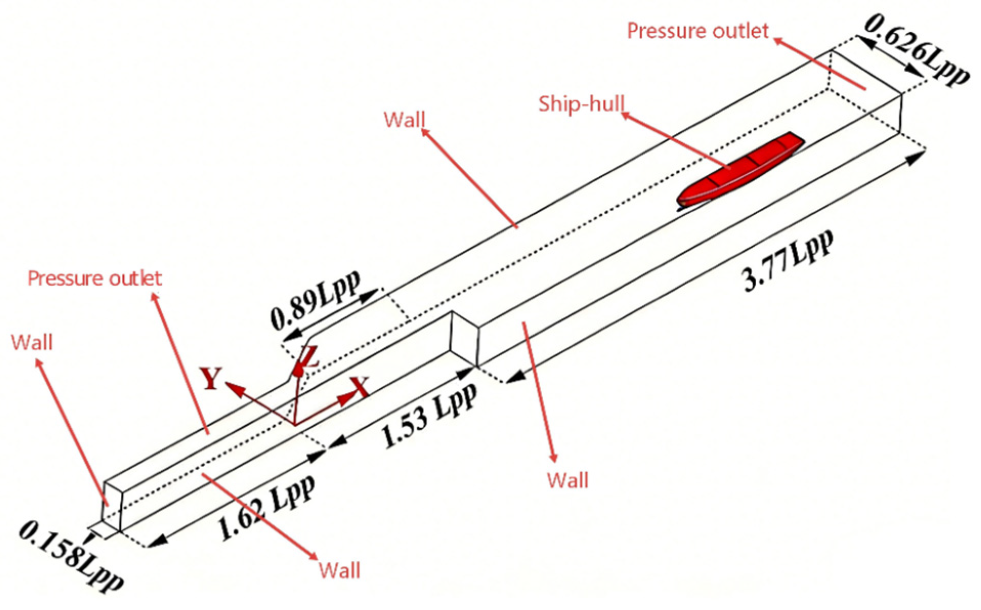
The computational domain and boundary conditions are shown in Figure 2. The CFD simulations are performed using STAR-CCM+. The overset mesh technique is adopted to describe the ship motion. The aft and top boundaries of the computational domain are set as pressure outlets, while the remaining boundaries are treated as no-slip walls. The realizable k-ε turbulence model is used, and the volume of fluid (VOF) method is employed to capture the free surface. The near-wall region is treated using the two-layer all y+ wall treatment, with (30 < y+ < 300). The maximum number of inner iterations is set to 10, and the time step is 0.02 s. The realizable k–ε model was selected because it provides a robust compromise between accuracy and computational cost for separated, rotational, and free-surface ship flows and is compatible with the two-layer all-y⁺ treatment over the present near-wall resolution. This balance is important because the CFD calculations are used to generate a multi-condition correction-force database rather than a single validation case.

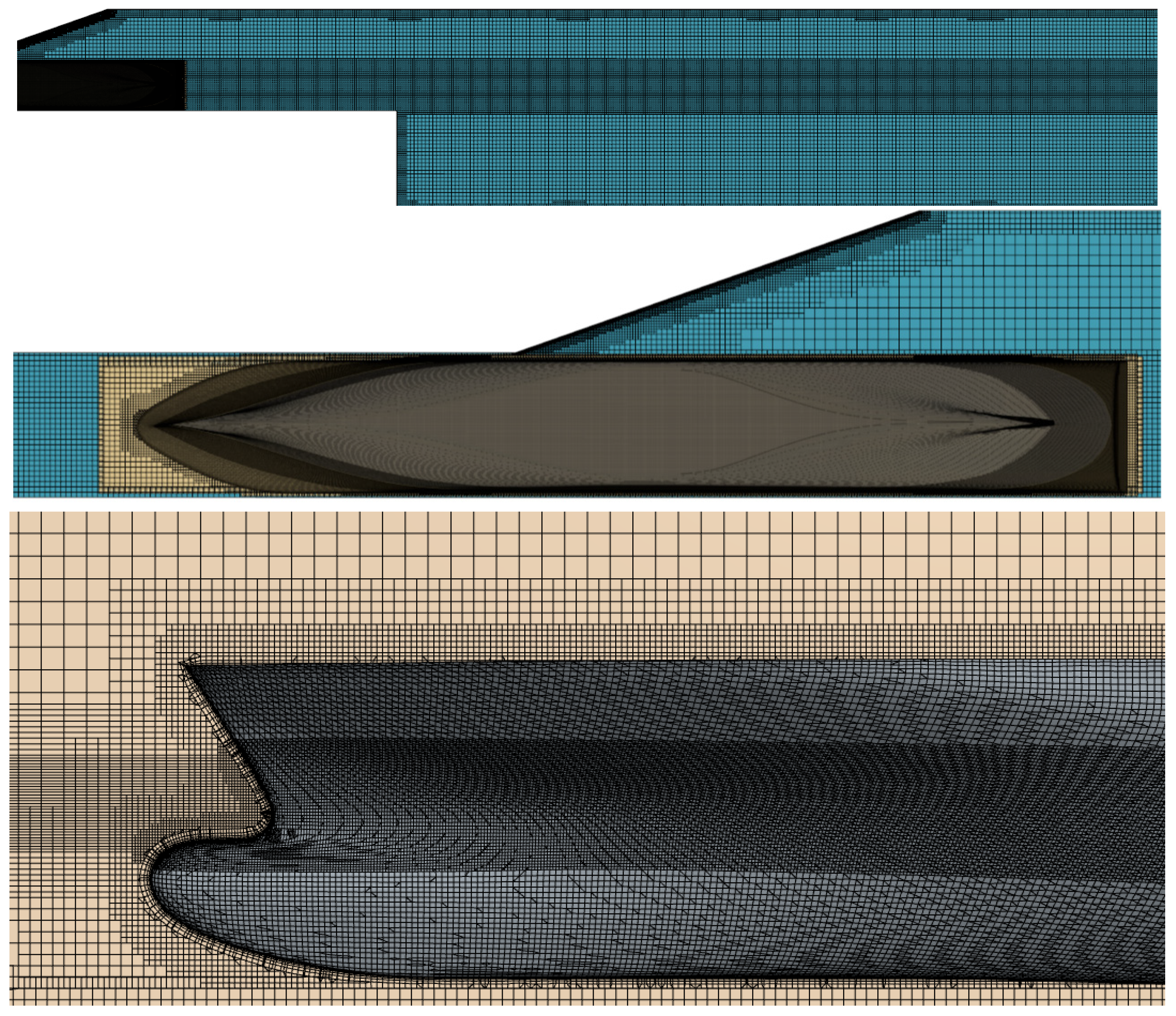
A mesh-sensitivity analysis was performed for the representative lock-entry validation condition using coarse, medium, and fine meshes containing approximately 4.5 million, 6.0 million, and 9.0 million cells, respectively. The medium mesh is shown in Figure 3. The mesh topology and local refinement regions near the hull, free surface, overset interface, and narrow hull–wall gap were kept consistent among the three meshes, while the physical models, boundary conditions, and solver settings remained unchanged.

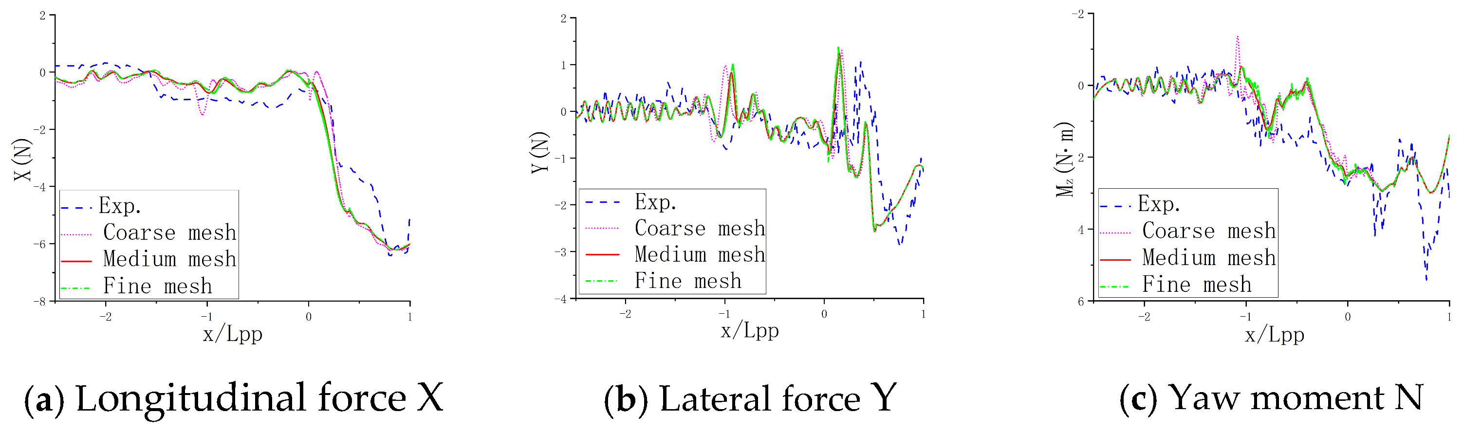
Figure 4 compares the longitudinal force X, lateral force Y, and yaw moment N obtained using the three meshes with the experimental measurements. All three meshes reproduce the overall magnitude and variation trends of the measured hydrodynamic loads, while the medium- and fine-mesh results are particularly close. The comparison provides a qualitative assessment of mesh sensitivity rather than a formal grid-convergence or numerical-uncertainty analysis. Because the predictions obtained using the medium and fine meshes are close over most of the investigated trajectory, the medium mesh was adopted as a compromise between computational cost and numerical resolution.

3.2. Design of Docking Conditions for Database Construction

After the CFD method is validated, a series of ship docking conditions are designed to construct the correction-force database. The database includes 23 CFD conditions in total: 20 model-development conditions and 3 independent holdout conditions. The full-scale dock dimensions are 280 m × 40 m × 13.6 m. Two representative hull forms are considered: a KCS container ship with $L_{pp}$ = 230 m and a rescaled KVLCC2-type tanker with $L_{pp}$ = 160 m. The original KVLCC2 hull form ($L_{pp}$ = 320 m) is uniformly rescaled in its principal dimensions by a factor of 0.5 to ensure compatibility with the selected dock geometry, while the loading-dependent variations in draft and displacement are specified separately in

Table 2. Ship-geometry-related input parameters.

Principal-Dimension Parameter ID	Ship Type	Displacement Volume	Breadth	Draft	Block Coefficient
		${\nabla }^{\mathbf{\prime }}$	${\mathit{B}}^{\mathbf{\prime }}$	${\mathit{d}}^{\mathbf{\prime }}$	Cb
A	KCS	0.0043	0.14	0.047	0.65
B		0.0017	0.14	0.019	0.65
C		0.0004	0.14	0.0047	0.65
D	KVLCC2	0.0095	0.18125	0.065	0.8098
E		0.00388	0.18125	0.026	0.8098
F		0.00095	0.18125	0.0065	0.8098

Note: The KVLCC2 hull form was uniformly rescaled in its principal dimensions by a factor of 0.5 before the loading-dependent draft and displacement variations were defined.

. Subsequently, a geometric scale ratio of 1:80 is applied in the CFD simulations, corresponding to model-scale ship lengths of 2.875 m for the KCS and 2.000 m for the rescaled KVLCC2.

The input feature vector $\mathit{\chi }=[{\nabla }^{\prime },B^{\prime },d^{\prime },C_{\mathrm{b}},x^{\prime },y^{\prime },\psi ,{\mathrm{F}\mathrm{r}}_U]$ used for SVR training consists of two groups of variables: ship-geometry-related parameters and docking-state-related parameters. The ship-geometry-related parameters include the dimensionless displacement volume, breadth, draft, and block coefficient. The docking-state-related parameters include the docking speed, heading angle, and lateral offset from the dock centerline.

The CFD correction database was constructed using prescribed constant-speed docking conditions. Within each condition, the reference speed $U$ was set equal to the initial longitudinal speed $U_0$, and u′ = 1 for all CFD samples. This design assumes that, during the investigated low-speed docking stage, the longitudinal speed varies gradually and the residual hydrodynamic corrections can be approximated using a quasi-steady formulation. Abrupt acceleration, rapid braking, and longitudinal-speed reversal are therefore outside the scope of the present database. Different reference-speed levels were included through ${\mathrm{F}\mathrm{r}}_U$ to represent the effect of docking speed while avoiding the substantially higher computational cost of continuously accelerated CFD simulations.

The ship-geometry-related parameter combinations are listed in Table 2. Six combinations are defined and denoted by A to F. These combinations cover different ship types and loading conditions, thereby providing variation in the main geometric parameters of the training samples.

The docking-state-related parameter combinations are listed in

Table 3. Docking-state-related input parameters.

Docking-Motion Parameter ID	Ship Type	Docking Speed, ${\mathbf{F}\mathbf{r}}_{\mathit{U}}$	Heading Angle, $\mathit{\psi }$ (°)	Offset from Centerline, ${\mathit{y}}^{\mathbf{\prime }}$
1	KCS	0.00105	0	0
2		0.00169	0	0
3		0.00169	1	0
4		0.00169	−1	0
5		0.00169	0	−0.002174
6		0.00169	0	0.002174
7	KVLCC2	0.00126	0	0
8		0.00202	0	0
9		0.00202	1	0
10		0.00202	−1	0
11		0.00202	0	−0.003125
12		0.00202	0	0.003125

. Twelve combinations are considered, including different docking speeds, heading angles, and lateral offsets for KCS and KVLCC2 ship hulls. These combinations are designed to represent typical low-speed docking states and small deviations from the dock centerline.

The training database is constructed by combining selected ship-geometry-related parameter sets with the docking-state-related parameter sets. For KCS, parameter sets A and B were combined with docking-state sets 1 and 2, whereas parameter set C was combined with sets 1–6. For KVLCC2, parameter sets D and E were combined with docking-state sets 7 and 8, whereas parameter set F was combined with sets 7–12. These combinations yielded 20 model-development conditions.

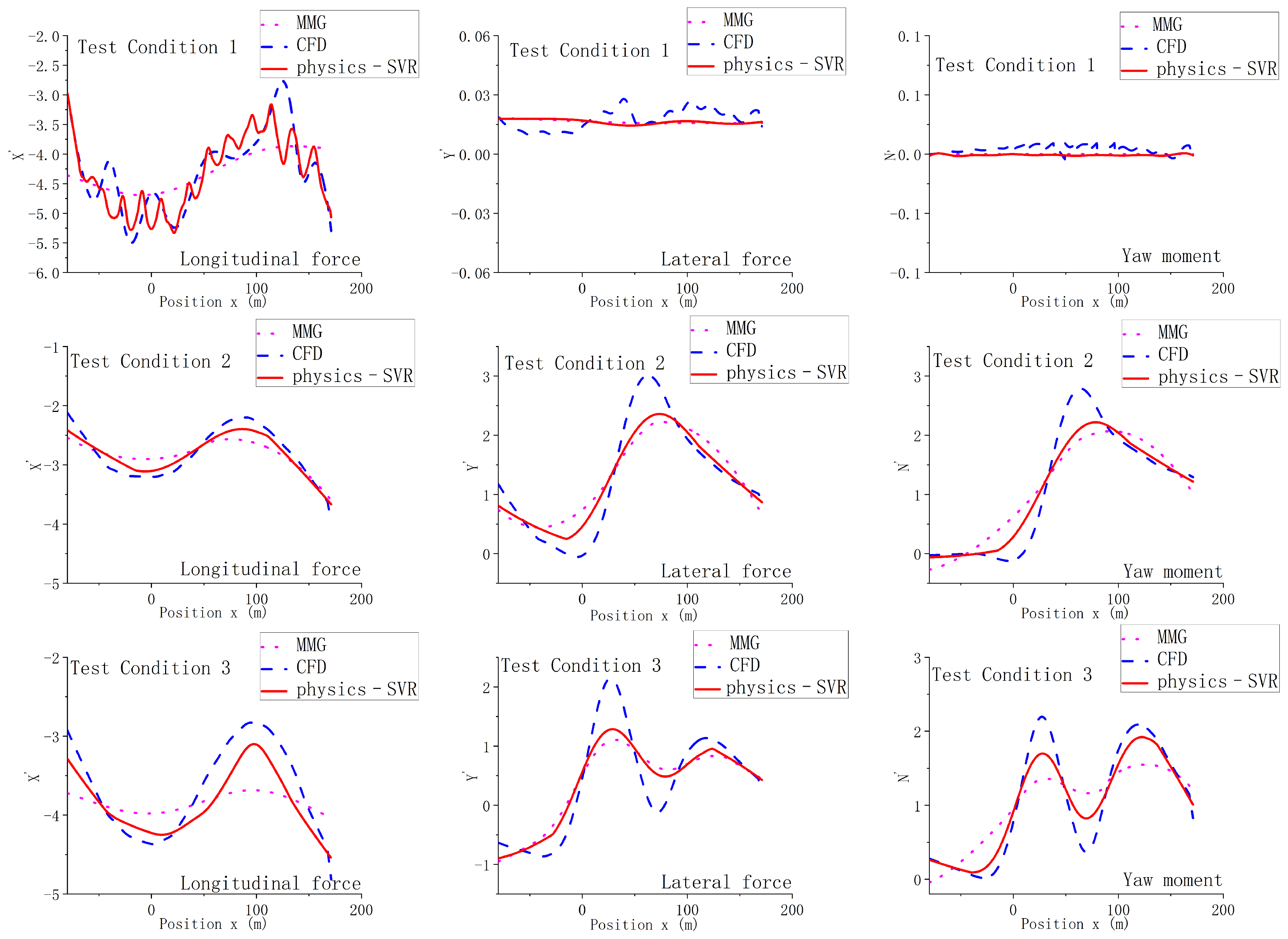
Three additional CFD conditions were excluded from all stages of model development and used only for condition-level holdout evaluation. The KVLCC2 tanker was used in all three holdout tests. Relative to the training conditions, Test 1 represents an unseen loading/draft combination, Test 2 an unseen heading angle, and Test 3 an unseen lateral offset. According to the feature order $\chi =[{\nabla }^{\prime },B^{\prime },d^{\prime },C_{\mathrm{b}},x^{\prime },y^{\prime },\psi ,{\mathrm{F}\mathrm{r}}_U]$, the input feature vectors for Tests 1–3 are [0.0019, 0.18125, 0.013, 0.8098, $x^{\prime }$, 0, 0, 0.00202], [0.00095, 0.18125, 0.0065, 0.8098, $x^{\prime }$, 0, 0.5, 0.00202] and [0.00095, 0.18125, 0.0065, 0.8098, $x^{\prime }$, 0.00125, 0, 0.00202], respectively, where $x^{\prime }$ denotes the instantaneous dimensionless longitudinal position and varies along each docking trajectory.

3.3. Extraction of Correction-Force Samples

For each docking condition, CFD simulations are conducted to obtain the longitudinal force, lateral force, and yaw moment at different ship positions during the docking process. The corresponding baseline physical-model predictions are then calculated using the method described in Section 2.3. The correction terms are obtained as the residuals between the CFD results and the baseline physical-model predictions:

$$\begin{gathered} {\delta X}_{\mathrm{t}\mathrm{r}\mathrm{a}\mathrm{i}\mathrm{n}}^{\prime }=X_{\mathrm{C}\mathrm{F}\mathrm{D}}^{\prime }-X_{\mathrm{P}\mathrm{M}}^{\prime } \\ \delta Y_{\mathrm{t}\mathrm{r}\mathrm{a}\mathrm{i}\mathrm{n}}^{\prime }=Y_{\mathrm{C}\mathrm{F}\mathrm{D}}^{\prime }-Y_{\mathrm{P}\mathrm{M}}^{\prime } \\ {\delta N}_{\mathrm{t}\mathrm{r}\mathrm{a}\mathrm{i}\mathrm{n}}^{\prime }=N_{\mathrm{C}\mathrm{F}\mathrm{D}}^{\prime }-N_{\mathrm{P}\mathrm{M}}^{\prime } \end{gathered}$$

(29)

For each sample, the input is the feature vector $\mathit{\chi }$, and the outputs are the three correction terms ${\delta X}_{\mathrm{t}\mathrm{r}\mathrm{a}\mathrm{i}\mathrm{n}}^{\prime }$, $\delta Y_{\mathrm{t}\mathrm{r}\mathrm{a}\mathrm{i}\mathrm{n}}^{\prime }$, and ${\delta N}_{\mathrm{t}\mathrm{r}\mathrm{a}\mathrm{i}\mathrm{n}}^{\prime }$. The correction-force database is therefore constructed in the following form:

$$[\chi , {\delta X}_{\mathrm{t}\mathrm{r}\mathrm{a}\mathrm{i}\mathrm{n}}^{\prime }, \delta Y_{\mathrm{t}\mathrm{r}\mathrm{a}\mathrm{i}\mathrm{n}}^{\prime }, {\delta N}_{\mathrm{t}\mathrm{r}\mathrm{a}\mathrm{i}\mathrm{n}}^{\prime }]$$

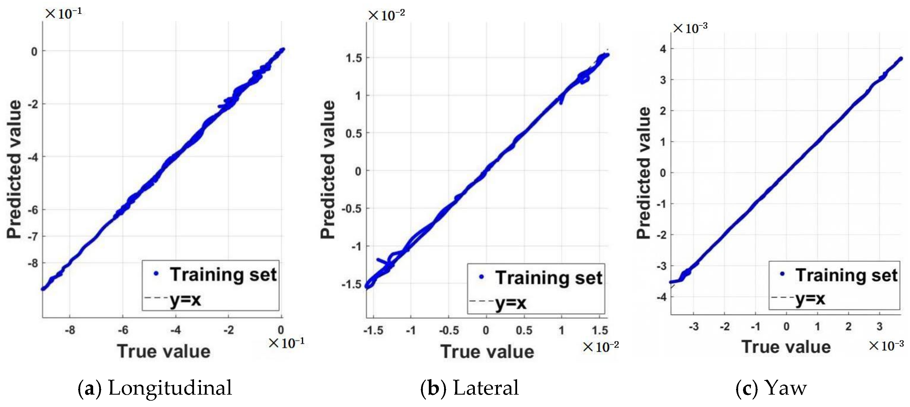
For the 20 training conditions, 2889 data samples are extracted from each condition, resulting in a total of 57,780 training samples. These samples are used to train the three SVR models for longitudinal force correction, lateral force correction, and yaw moment correction, respectively. Although 2889 data samples were extracted from each CFD simulation, the samples within the same docking condition belong to a continuous physical trajectory and are strongly correlated. Therefore, the effective number of independent observations is determined primarily by the number of physical docking conditions rather than by the total number of extracted data points.

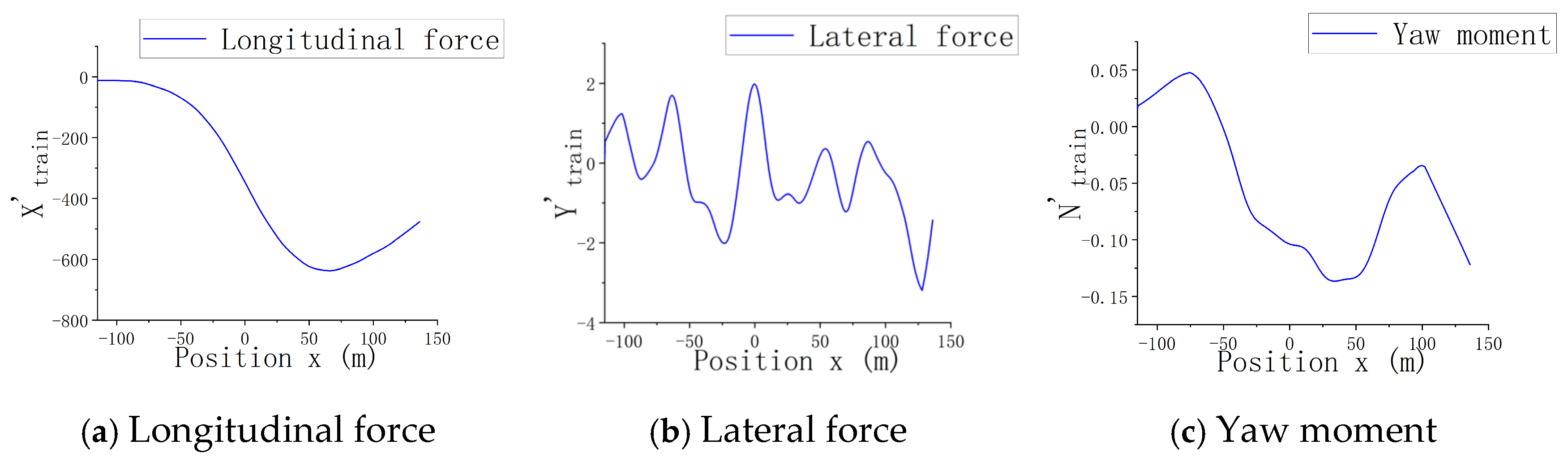
The correction-force database comprises 23 independent CFD docking conditions, and each condition contains a large number of data samples extracted at successive ship positions during the docking process. Presenting the correction-force histories for all conditions would be repetitive and would require excessive space. Therefore, one representative condition is selected to illustrate the structure and variation characteristics of the extracted residual data. For this condition, the ship-geometry-related parameters correspond to set B in Table 2, and the docking-state-related parameters correspond to set 2 in Table 3. The resulting longitudinal-force, lateral-force, and yaw-moment correction terms are shown in Figure 5.

4. Training and Validation of the Physics–SVR Model

4.1. Data Preprocessing and Hyperparameter Selection

Based on the CFD-based correction-force database constructed in Section 3, three SVR models are trained to predict the correction terms for the longitudinal force, lateral force, and yaw moment, respectively. The input of each SVR model is the feature vector $\mathit{\chi }$, which includes both ship-geometry-related parameters and docking-state-related parameters. The outputs are the physical-model residuals $\delta X_{\mathrm{S}\mathrm{V}\mathrm{R}}^{\prime },\delta Y_{\mathrm{S}\mathrm{V}\mathrm{R}}^{\prime },\delta N_{\mathrm{S}\mathrm{V}\mathrm{R}}^{\prime }$, as defined in Equation (24).

The training is performed using the correction-force samples extracted from the 20 training conditions. After training, the predicted correction terms are superimposed onto the baseline physical-model results according to Equation (26), thereby obtaining the final force and moment predictions of the physics–SVR model. The final optimized hyperparameter settings are summarized in

Table 4. Hyperparameter settings of the three SVR correction models.

SVR Output	BoxConstraint, $\mathit{C}$	Epsilon, $\mathit{\epsilon }$	KernelScale, ${\mathit{\sigma }}_{\mathit{k}}$
Longitudinal-force correction, ${\delta X}_{\mathrm{S}\mathrm{V}\mathrm{R}}^{\prime }$	0.2193	0.045182	1.1026
Lateral-force correction, ${\delta Y}_{\mathrm{S}\mathrm{V}\mathrm{R}}^{\prime }$	0.5779	0.002203	1.3668
Yaw-moment correction, ${\delta N}_{\mathrm{S}\mathrm{V}\mathrm{R}}^{\prime }$	1.3824	0.000292	4.5221

.

The 20 docking conditions used to construct the correction-force database are treated as the model-development dataset, whereas the three independent holdout conditions described in Section 3.2 are excluded from all preprocessing and hyperparameter selection. All three models use the Gaussian radial basis function kernel, and predictor standardization is enabled (Standardize = true). To avoid information leakage between highly correlated samples extracted from the same CFD trajectory, the cross-validation folds are formed by docking condition rather than by randomly assigning individual samples.

For each output component, BoxConstraint C, Epsilon ε, and KernelScale σ_k are optimized independently using Bayesian optimization with five-fold condition-grouped cross-validation. The optimization minimizes the mean cross-validation mean-squared error. Logarithmic search ranges of ${10}^{-3}-{10}^3$ are used for both C and σ_k; the search range for ε is [10⁻³, 10²] × IQR(y)/1.349, where IQR(y) is the interquartile range of the corresponding response in the training fold. The expected-improvement-plus acquisition function, a maximum of 30 objective evaluations, and a fixed random seed are adopted to ensure reproducibility. After optimization, each SVR model is retrained using all samples from the 20 training conditions with its selected hyperparameters.

4.2. Model Fitting Performance

Figure 6 and

Table 5. Training-set correlation coefficients of the three SVR correction models.

Evaluation Index	Surge Force	Sway Force	Yaw Moment
Training-set performance	0.99978	0.99988	0.99988

describe the fitting performance of the three SVR models on the model-development database. The correlation coefficients close to unity indicate that the SVR models can reproduce the residual patterns contained in the training data. However, these training-set statistics should not be interpreted as evidence of model generalization, because samples extracted from the same CFD docking trajectory are strongly correlated and have already contributed to model fitting. The generalization performance is therefore evaluated separately using complete docking conditions that are excluded from all stages of model development, as described in Section 4.3.

The correlation coefficients between the CFD-derived correction terms and the SVR-predicted correction terms are listed in Table 5. The coefficients for the longitudinal-force, lateral-force, and yaw-moment corrections are all close to unity, indicating strong fitting performance on the model-development database; they are not interpreted as evidence of generalization.

4.3. Holdout Evaluation Under Three Withheld Docking Conditions

Three complete CFD docking conditions were withheld from all stages of model development and used only for condition-level evaluation. Each holdout case represents a previously unseen parameter combination within the ranges covered by the model-development dataset. Therefore, these tests assess predictive performance for withheld conditions within the investigated parameter domain rather than extrapolation to new hull forms, dock geometries, or operating ranges.

To quantify the incremental benefit of the SVR residual correction, the baseline physical model and the physics–SVR model were evaluated under identical holdout conditions using the same ship states, predictor inputs, sample locations, and CFD reference data. The baseline predictions were obtained directly from the MMG-based physical model, whereas the physics–SVR predictions were obtained by adding the SVR-predicted residuals according to Equation (26). Therefore, differences between the two sets of results directly reflect the contribution of the data-driven residual correction.

Figure 7 compares the baseline physical-model results, CFD reference data, and physics–SVR predictions for all three independent holdout conditions. The rows correspond to Tests 1–3, respectively, while the columns show the longitudinal force X′, lateral force Y′, and yaw moment N′. For Test 1, the SVR correction provides a modest improvement in X′ and Y′ and a clearer improvement in N′. For Tests 2 and 3, the physics–SVR curves follow the CFD reference more closely across all three hydrodynamic components, particularly around the main peaks and changes in the lateral force and yaw moment. These comparisons indicate that the benefit of the residual correction is condition-dependent but is consistently positive across the three holdout cases.

For quantitative assessment, the relative error of each hydrodynamic component q is calculated from the accumulated absolute deviation between the model prediction and the CFD reference over all n samples in each holdout condition:

$$E_q=\left[{\displaystyle \frac{{\displaystyle {\sum }_{i=1}^n}\left|q_{\mathrm{m}\mathrm{o}\mathrm{d}\mathrm{e}\mathrm{l},i}-q_{\mathrm{C}\mathrm{F}\mathrm{D},i}\right|}{{\displaystyle {\sum }_{i=1}^n}\left|q_{\mathrm{C}\mathrm{F}\mathrm{D},i}\right|}}\right]\times 100\%$$

where q denotes X′, Y′, or N′, and the subscripts “model” and “CFD” denote the evaluated model and CFD reference, respectively. The overall relative error is defined as the arithmetic mean of the three component-wise errors:

$$E_{\mathrm{o}\mathrm{v}\mathrm{e}\mathrm{r}\mathrm{a}\mathrm{l}\mathrm{l}}={\displaystyle \frac{E_{X^{\prime }}+E_{Y^{\prime }}+E_{N^{\prime }}}{3}}$$

The improvement introduced by the SVR correction is further quantified by the relative reduction in the overall error:

$$\eta =\left[{\displaystyle \frac{E_{\mathrm{b}\mathrm{a}\mathrm{s}\mathrm{e}\mathrm{l}\mathrm{i}\mathrm{n}\mathrm{e}}-E_{\mathrm{p}\mathrm{h}\mathrm{y}\mathrm{s}\mathrm{i}\mathrm{c}\mathrm{s}-\mathrm{S}\mathrm{V}\mathrm{R}}}{E_{\mathrm{b}\mathrm{a}\mathrm{s}\mathrm{e}\mathrm{l}\mathrm{i}\mathrm{n}\mathrm{e}}}}\right]\times 100\%$$

As summarized in

Table 6. Direct comparison of the baseline physical model and the physics–SVR model under independent holdout conditions.

Holdout Condition	Model	Relative Error in X′ (%)	Relative Error in Y′ (%)	Relative Error in N′ (%)	Overall Relative Error (%)
Test 1 (unseen draft)	Baseline physical model	9.75	31.98	30.21	23.98
	Physics–SVR model	8.78	30.82	19.24	19.61
Test 2 (unseen heading angle)	Baseline physical model	8.49	28.78	28.75	22.00
	Physics–SVR model	4.62	20.86	19.24	14.91
Test 3 (unseen lateral offset)	Baseline physical model	12.74	44.54	33.34	30.20
	Physics–SVR model	7.46	36.11	16.21	19.93

, the overall relative errors of the baseline physical model are 23.98%, 22.00%, and 30.20% for Tests 1–3, respectively. After the SVR residual correction, these values decrease to 19.61%, 14.91%, and 19.93%, corresponding to relative error reductions of 18.22%, 32.23%, and 34.01%. The smallest improvement occurs in Test 1, where the lateral-force error changes only slightly from 31.98% to 30.82%; however, the yaw-moment error is reduced from 30.21% to 19.24%. In Test 2, the errors in X′, Y′, and N′ decrease from 8.49%, 28.78%, and 28.75% to 4.62%, 20.86%, and 19.24%, respectively. In Test 3, the corresponding errors decrease from 12.74%, 44.54%, and 33.34% to 7.46%, 36.11%, and 16.21%. The larger overall reductions in Tests 2 and 3 show that the residual correction is particularly effective for the unseen heading-angle and lateral-offset conditions considered here.

Taken together, the three condition-level holdout tests provide a substantially more stringent assessment of model generalization than the near-unity training-set correlation coefficients reported in Section 4.2, because each test consists of a complete CFD trajectory that was never used during model development. The results demonstrate that the physics–SVR correction improves the baseline hydrodynamic predictions for three distinct types of previously unseen docking conditions. Nevertheless, the holdout set remains limited in both size and parameter coverage. The present results therefore support generalization only within the investigated ship types, dock geometry, and operating ranges; additional CFD cases, dedicated dry-dock model tests, and full-scale docking measurements are still required before broader engineering application.

5. Ship Docking Collision-Risk Early-Warning Model Based on Physics–SVR Motion Prediction

Based on the physics–SVR motion prediction model established in the previous sections, a collision-risk early-warning model was further developed for ship docking. The basic idea is to predict the future trajectory of the ship within a specified time window and then evaluate the collision risk according to the minimum clearance between the predicted hull envelope and the dock chamber boundaries.

5.1. Overall Workflow of the Collision-Risk Early-Warning Model

The proposed method is primarily intended for integration into a shore-based docking-assistance system that provides real-time warning information and decision support for dock operators. In practical use, the current ship position, heading, velocity, and yaw rate may be obtained from available ship–shore monitoring and positioning systems, while the ship particulars and dock geometry are stored in advance. The physics–SVR model predicts the future ship trajectory and evaluates the lateral and longitudinal clearances to the dock boundaries. The resulting warning information is presented to the operator, who remains responsible for determining the appropriate operational response in combination with tug capability, positioning-system status, environmental conditions, and established docking procedures.

During ship docking, the instantaneous ship position, heading, and velocity components are updated at each time step. The SVR input vector χ(t) is constructed using the ship particulars, the instantaneous position and heading [x′(t), y′(t), ψ(t)], and the reference-speed parameter ${\mathrm{F}\mathrm{r}}_U$. The instantaneous velocity components u(t), v(t), and r(t) are used in the 3-DOF physical model but are not included as independent SVR predictors. The trained physics–SVR model then predicts the hydrodynamic force and moment, and the future ship trajectory is obtained by solving the 3-DOF equations of motion.

After the future trajectory is predicted, the hull envelope is reconstructed at each predicted time instant. The minimum clearances between the hull envelope and the left dock wall, right dock wall, and dock end are then calculated. Based on these distances, the lateral collision risk and longitudinal collision risk are evaluated separately. Finally, the warning status is determined according to the predefined warning criteria.

In the present numerical verification, the prediction horizon is set to $T_{\mathrm{p}}$ = 120 s. This two-minute horizon was selected as a scenario-specific compromise: it provides sufficient look-ahead for operators to identify a developing risk, communicate instructions, and initiate tug or positioning-system intervention, while limiting the accumulation of uncertainty in longer-horizon motion prediction. It is used for proof-of-concept validation rather than as a universal operational setting.

In practical applications, $T_{\mathrm{p}}$ should be calibrated according to ship length, docking speed, remaining clearance, operator reaction time, tug or positioning-system response, and available stopping distance. Larger or faster ships and slower response systems generally require a longer horizon. Because full-scale response-time and stopping-distance data were unavailable, further calibration using shipyard operational data is required before practical deployment.

5.2. Calculation of the Minimum Clearance Between the Hull Envelope and the Dock Chamber Boundary

During ship docking, collision risk is evaluated according to the clearance between the hull and the dock chamber boundaries. In this study, the hull contour in the horizontal plane is approximated by a rectangular envelope. The four characteristic points of the hull envelope are expressed as

$$x_i=x_0+{\epsilon }_i{\displaystyle \frac{L}{2}}\mathrm{c}\mathrm{o}\mathrm{s}\psi -{\nu }_i{\displaystyle \frac{B}{2}}\mathrm{s}\mathrm{i}\mathrm{n}\psi$$

(30a)

$$y_i=y_0+{\epsilon }_i{\displaystyle \frac{L}{2}}\mathrm{s}\mathrm{i}\mathrm{n}\psi +{\nu }_i{\displaystyle \frac{B}{2}}\mathrm{c}\mathrm{o}\mathrm{s}\psi , i=\mathrm{1,2},\mathrm{3,4}$$

(30b)

where (x₀, y₀) is the predicted or measured position of the ship center, ψ is the heading angle, and L and B are the ship length and breadth. The corner-marker coefficient pairs are defined, without repetition, as (ε₁, ν₁) = (1, 1), (ε₂, ν₂) = (1, −1), (ε₃, ν₃) = (−1, −1), and (ε₄, ν₄) = (−1, 1), corresponding respectively to the four corners of the rectangular hull envelope.

At each predicted time instant, the lateral clearance to the left and right dock walls and the longitudinal clearance to the dock end are calculated from the four hull-envelope points. The instantaneous minimum lateral clearance and longitudinal clearance are denoted as ${ D}_{\mathrm{l}\mathrm{a}\mathrm{t}}\left(\tau \right)$ and $D_{\mathrm{l}\mathrm{o}\mathrm{n}}\left(\tau \right)$, respectively.

Within the prediction time window T_p, the minimum predicted lateral and longitudinal clearances are defined as

$$D_{\mathrm{l}\mathrm{a}\mathrm{t}}^{\mathrm{p}}\left(t\right)=\underset{0\le \tau \le T_{\mathrm{p}}}{\mathrm{m}\mathrm{i}\mathrm{n}}{D}_{\mathrm{l}\mathrm{a}\mathrm{t}}\left(t+\tau \right)$$

(31a)

$$D_{\mathrm{l}\mathrm{o}\mathrm{n}}^{\mathrm{p}}\left(t\right)=\underset{0\le \tau \le T_{\mathrm{p}}}{\mathrm{m}\mathrm{i}\mathrm{n}}{D}_{\mathrm{l}\mathrm{o}\mathrm{n}}\left(t+\tau \right)$$

(31b)

Here, $D_{\mathrm{l}\mathrm{a}\mathrm{t}}^{\mathrm{p}}\left(t\right)$ and $D_{\mathrm{l}\mathrm{o}\mathrm{n}}^{\mathrm{p}}\left(t\right)$ are the minimum predicted lateral and longitudinal clearances over the future horizon $0\le \tau \le T_{\mathrm{p}}$. The use of the same prediction-offset variable $\tau$ in Equations (31a)–(31e) ensures consistent notation.

In addition to the minimum predicted clearances, the first future instant at which either predicted clearance reaches its corresponding safety threshold is calculated to characterize the temporal urgency of the risk. The lateral and longitudinal times to threshold are defined as follows:

$$T_{\mathrm{l}\mathrm{a}\mathrm{t}}^{\mathrm{t}\mathrm{h}}\left(t\right)=\mathrm{i}\mathrm{n}\mathrm{f}\left\{\tau \in (0,T_{\mathrm{p}}]:D_{\mathrm{l}\mathrm{a}\mathrm{t}}\left(t+\tau \right)\le D_{\mathrm{l}\mathrm{a}\mathrm{t}}^{\mathrm{s}\mathrm{a}\mathrm{f}\mathrm{e}}\right\}$$

(31c)

$$T_{\mathrm{l}\mathrm{o}\mathrm{n}}^{\mathrm{t}\mathrm{h}}\left(t\right)=\mathrm{i}\mathrm{n}\mathrm{f}\left\{\tau \in (0,T_{\mathrm{p}}]:D_{\mathrm{l}\mathrm{o}\mathrm{n}}\left(t+\tau \right)\le D_{\mathrm{l}\mathrm{o}\mathrm{n}}^{\mathrm{s}\mathrm{a}\mathrm{f}\mathrm{e}}\right\}$$

(31d)

$$T_{\mathrm{t}\mathrm{h}}\left(t\right)=\mathrm{m}\mathrm{i}\mathrm{n}\left[T_{\mathrm{l}\mathrm{a}\mathrm{t}}^{\mathrm{t}\mathrm{h}}\left(t\right),T_{\mathrm{l}\mathrm{o}\mathrm{n}}^{\mathrm{t}\mathrm{h}}\left(t\right)\right]$$

(31e)

If a predicted clearance does not reach its safety threshold within the prediction horizon, the corresponding time to threshold is assigned as +∞. The overall time to threshold is the earlier of the lateral and longitudinal values and therefore represents the earliest predicted entry into either unsafe-clearance region. Thus, the minimum predicted clearance characterizes spatial severity, whereas the time to threshold characterizes temporal urgency.

The rectangular representation is adopted as a computationally efficient approximation for repeated clearance evaluation over the prediction horizon. In the present implementation, the rectangle is treated as an outer envelope defined by the selected ship length and breadth. It therefore generally gives a minimum clearance that is no greater than that obtained from the actual plan-view hull contour, providing a conservative basis for warning. The approximation becomes more conservative when a heading deviation exists because the rectangular bow and stern corners project toward the dock boundaries, whereas the actual bow and stern contours are tapered. Consequently, the rectangular envelope may underestimate the actual clearance and trigger the warning earlier, particularly as the heading deviation increases. It is therefore intended for conservative risk screening rather than exact geometric clearance estimation. For applications requiring higher geometric fidelity, the same framework can replace the rectangle with a polygonal waterline contour or a CAD-derived hull boundary without changing the motion-prediction and warning logic.

5.3. Warning Criteria

During ship docking, collision risk is evaluated separately in the lateral and longitudinal directions. Lateral risk refers to the possibility that the hull approaches or contacts either dock wall, whereas longitudinal risk refers to the possibility that the bow approaches or contacts the dock end. The instantaneous lateral and longitudinal clearances are denoted by $D_{\mathrm{l}\mathrm{a}\mathrm{t}}\left(t\right)$, and $D_{\mathrm{l}\mathrm{o}\mathrm{n}}\left(t\right)$, respectively. The minimum clearances predicted over the future horizon are denoted by $D_{\mathrm{l}\mathrm{a}\mathrm{t}}^{\mathrm{p}}\left(t\right)$ and $D_{\mathrm{l}\mathrm{o}\mathrm{n}}^{\mathrm{p}}\left(t\right)$. The corresponding safety thresholds are $D_{\mathrm{l}\mathrm{a}\mathrm{t}}^{\mathrm{s}\mathrm{a}\mathrm{f}\mathrm{e}}$ and $D_{\mathrm{l}\mathrm{o}\mathrm{n}}^{\mathrm{s}\mathrm{a}\mathrm{f}\mathrm{e}}$.

The thresholds used in the present study are scenario-specific engineering margins rather than universal regulatory limits. For the KCS-based warning-validation cases, the full-scale ship length and breadth are $L=230 \mathrm{m}$ and $B=32.2 \mathrm{m}$, while the dock chamber length and width are $L_{\mathrm{d}}=280 \mathrm{m}$ and $W_{\mathrm{d}}=40 \mathrm{m}$, respectively. When the ship is centered and aligned with the dock, the nominal one-side lateral clearance and longitudinal geometric allowance are

$$C_{\mathrm{l}\mathrm{a}\mathrm{t},0}={\displaystyle \frac{W_{\mathrm{d}}-B}{2}}={\displaystyle \frac{40-32.2}{2}}=3.9 \mathrm{m},$$

$$C_{\mathrm{l}\mathrm{o}\mathrm{n},0}=L_{\mathrm{d}}-\mathrm{L}=280-230=50 \mathrm{m}.$$

Accordingly, the lateral threshold of $1\mathrm{m}$ corresponds to approximately $25.6\%$ of the nominal one-side lateral clearance, while the longitudinal threshold of $10\mathrm{m}$ corresponds to $20\%$ of the available longitudinal allowance. These ratios provide a transparent geometric basis for the selected values, but they should not be interpreted as generally applicable safety factors.

The difference between the two absolute thresholds reflects the different operational characteristics of lateral and longitudinal risk. Lateral motion develops within a relatively small side clearance and is directly associated with hull–wall proximity. Longitudinal risk, by contrast, involves the forward inertia of the ship and requires sufficient distance for command communication, tug-force development, positioning-device actuation, and operator intervention. A larger absolute longitudinal margin is therefore adopted. Nevertheless, because tug and positioning-system dynamics and measured response times are not included in the present model, the $10\hspace{0.25em}m$ threshold represents a qualitative operational allowance rather than a value derived from a calibrated stopping-distance model.

For application to other ship–dock combinations, the thresholds may be expressed in a normalized form as

$$D_{\mathrm{l}\mathrm{a}\mathrm{t}}^{\mathrm{s}\mathrm{a}\mathrm{f}\mathrm{e}}={\kappa }_{\mathrm{l}\mathrm{a}\mathrm{t}}{\displaystyle \frac{W_{\mathrm{d}}-B}{2}},$$

$$D_{\mathrm{l}\mathrm{o}\mathrm{n}}^{\mathrm{s}\mathrm{a}\mathrm{f}\mathrm{e}}={\kappa }_{\mathrm{l}\mathrm{o}\mathrm{n}}\left(L_{\mathrm{d}}-L\right),$$

where ${\kappa }_{\mathrm{l}\mathrm{a}\mathrm{t}}$ and ${\kappa }_{\mathrm{l}\mathrm{o}\mathrm{n}}$ are operational safety factors. For the present numerical verification, ${\kappa }_{\mathrm{l}\mathrm{a}\mathrm{t}}\approx 0.26$ and ${\kappa }_{\mathrm{l}\mathrm{o}\mathrm{n}}=0.20$ are adopted. Before practical implementation, these factors should be recalibrated using the actual ship dimensions, dock geometry, approach speed, stopping characteristics, tug or positioning-system capability, communication and actuation delays, measurement uncertainty, prediction uncertainty, environmental disturbances, and shipyard operating procedures. The adopted warning thresholds and their physical interpretations are summarized in Table 7.

Table 7. Warning-threshold settings.

Risk Category	Safety Threshold	Physical Meaning
Lateral risk	$D_{\mathrm{l}\mathrm{a}\mathrm{t}}^{\mathrm{s}\mathrm{a}\mathrm{f}\mathrm{e}}=1 \mathrm{m}$	Scenario-specific margin: 1 m is approximately 26% of the nominal one-side lateral clearance of 3.9 m for the KCS in the 40 m-wide dock.
Longitudinal risk	$D_{\mathrm{l}\mathrm{o}\mathrm{n}}^{\mathrm{s}\mathrm{a}\mathrm{f}\mathrm{e}}=10 \mathrm{m}$	Scenario-specific margin: 10 m is 20% of the 50 m longitudinal geometric allowance; the larger absolute value provides stopping and operational-response margin.

Table 7. Warning-threshold settings.

Risk Category	Safety Threshold	Physical Meaning
Lateral risk	$D_{\mathrm{l}\mathrm{a}\mathrm{t}}^{\mathrm{s}\mathrm{a}\mathrm{f}\mathrm{e}}=1 \mathrm{m}$	Scenario-specific margin: 1 m is approximately 26% of the nominal one-side lateral clearance of 3.9 m for the KCS in the 40 m-wide dock.
Longitudinal risk	$D_{\mathrm{l}\mathrm{o}\mathrm{n}}^{\mathrm{s}\mathrm{a}\mathrm{f}\mathrm{e}}=10 \mathrm{m}$	Scenario-specific margin: 10 m is 20% of the 50 m longitudinal geometric allowance; the larger absolute value provides stopping and operational-response margin.

Based on these thresholds, the docking state is classified as normal, warning alert, or emergency alarm. A warning alert is issued only when the current clearance remains outside the unsafe region but the predicted minimum clearance crosses the corresponding threshold within the prediction horizon. This definition separates a predictive warning from an emergency condition that has already occurred.

$$D_{\mathrm{l}\mathrm{a}\mathrm{t}}\left(t\right)\ge D_{\mathrm{l}\mathrm{a}\mathrm{t}}^{\mathrm{s}\mathrm{a}\mathrm{f}\mathrm{e}} \mathrm{a}\mathrm{n}\mathrm{d} D_{\mathrm{l}\mathrm{a}\mathrm{t}}^{\mathrm{p}}\left(t\right)<D_{\mathrm{l}\mathrm{a}\mathrm{t}}^{\mathrm{s}\mathrm{a}\mathrm{f}\mathrm{e}}$$

(32a)

$$D_{\mathrm{l}\mathrm{o}\mathrm{n}}\left(t\right)\ge D_{\mathrm{l}\mathrm{o}\mathrm{n}}^{\mathrm{s}\mathrm{a}\mathrm{f}\mathrm{e}} \mathrm{a}\mathrm{n}\mathrm{d} D_{\mathrm{l}\mathrm{o}\mathrm{n}}^{\mathrm{p}}\left(t\right)<D_{\mathrm{l}\mathrm{o}\mathrm{n}}^{\mathrm{s}\mathrm{a}\mathrm{f}\mathrm{e}}$$

(32b)

When either condition in Equation (32a) or Equation (32b) is satisfied, the first predicted time at which a safety threshold is reached must lie within the selected prediction horizon:

$$T_{\mathrm{t}\mathrm{h}}\left(t\right)\le T_{\mathrm{p}}$$

(32c)

The emergency alarm is determined from the instantaneous clearances and is activated when the hull has already entered either unsafe-clearance region:

$$D_{\mathrm{l}\mathrm{a}\mathrm{t}}\left(t\right)<D_{\mathrm{l}\mathrm{a}\mathrm{t}}^{\mathrm{s}\mathrm{a}\mathrm{f}\mathrm{e}} \mathrm{o}\mathrm{r} D_{\mathrm{l}\mathrm{o}\mathrm{n}}\left(t\right)<D_{\mathrm{l}\mathrm{o}\mathrm{n}}^{\mathrm{s}\mathrm{a}\mathrm{f}\mathrm{e}}.$$

(32d)

When the emergency alarm is activated, $T_{\mathrm{t}\mathrm{h}}\left(t\right)$ is taken as zero. If no threshold crossing is predicted within $T_{\mathrm{p}}$, the corresponding time to threshold is assigned as $+\mathrm{\infty }$. The warning output therefore includes the dominant risk direction, the minimum predicted clearance, and the time to threshold. The minimum clearance characterizes spatial severity, whereas the time to threshold characterizes temporal urgency. Inspired by the spatiotemporal risk-inference concept in [38], this combination provides dock operators with both the magnitude of the boundary-approach risk and the time available for operational response.

Under this classification, the normal state applies when neither the predictive-warning conditions nor the emergency condition is satisfied. The adopted logic therefore avoids simultaneous classification as warning and emergency and provides a clear progression from normal operation to predicted risk and, finally, to immediate danger.

5.4. Validation of the Collision-Risk Early-Warning Model

To validate the proposed collision-risk early-warning model, three warning-validation conditions are selected for numerical verification. In each validation case, the CFD simulation results are used as the reference trajectory and contact-time data. During the verification process, the current ship state is updated according to the CFD simulation results. At each prediction update, the SVR input vector χ(t) is constructed using the current position and heading, while Fr_U remains fixed at the value corresponding to the initial/reference docking speed. The instantaneous velocity components u(t), v(t), and r(t) are updated through the 3-DOF equations but are not supplied as independent SVR predictors. The coupled physics–SVR equations are then solved to predict the ship trajectory over the subsequent 120 s.

Based on the predicted trajectory, the hull envelope is reconstructed, and the minimum lateral and longitudinal clearances and times to threshold are calculated according to Equations (30a)–(31e). The warning status is then determined using the criteria in Section 5.3. The warning results are compared with the CFD-based reference contact time to evaluate whether the proposed model identifies the risk before physical contact.

The present proof-of-concept evaluation focuses on whether the warning states are activated before the CFD-reference contact and on the associated warning lead times. The minimum predicted clearances and times to threshold are calculated internally as part of the warning-state determination but are not reported separately in the present evaluation. Accordingly, the results are summarized in terms of the warning-alert time, emergency-alarm time, contact time, and the corresponding lead times.

Three warning-validation conditions are considered, including two hazardous cases and one non-hazardous control case. For condition 1, the principal-dimension vector is [${\nabla }^{\prime }=0.0004, B^{\prime }=0.14, d^{\prime }=0.0047, C_{\mathrm{b}}=0.65$]; the initial motion-state vector is [$y^{\prime }=0,\psi ={0.5}^{°}, {\mathrm{F}\mathrm{r}}_U=0.00421$]. For condition 2, the principal-dimension vector is [${\nabla }^{\prime }=0.0004, B^{\prime }=0.14, d^{\prime }=0.0047, C_{\mathrm{b}}=0.65$]; the initial motion-state vector is [$y^{\prime }=0.002174,\psi =1^{°}, {\mathrm{F}\mathrm{r}}_U=0.00421$]. For condition 3, the principal-dimension vector is [${\nabla }^{\prime }=0.0004, B^{\prime }=0.14, d^{\prime }=0.0047, C_{\mathrm{b}}=0.65$]; the initial motion-state vector is [$y^{\prime }=0,\psi =0^{°}, {\mathrm{F}\mathrm{r}}_U=0.00421$].

The verification results show that for warning-validation condition 1, the warning alert is issued at t = 1240.2 s, the emergency alarm is triggered at t = 1350.1 s, and contact occurs at t = 1395.1 s. Therefore, the warning-alert lead time is 154.9 s, and the emergency-alarm lead time is 45.0 s. In warning-validation condition 2, the warning alert is issued at t = 632.6 s, the emergency alarm is triggered at t = 688.2 s, and contact occurs at t = 804.69 s. Therefore, the warning-alert lead time is 172.09 s, and the emergency-alarm lead time is 116.49 s. The warning-alert and emergency-alarm lead times are calculated relative to the CFD-reference contact time. It should be noted that the warning-alert lead time may exceed the 120 s prediction horizon. This is because the warning alert is activated when the model predicts that a safety threshold will be crossed within the subsequent 120 s, whereas physical contact with the dock boundary may occur later than the safety-threshold crossing. The validation results are summarized in

Table 8. Timing results for the three warning-evaluation conditions.

Condition	Contact Time (s)	Warning-Alert Time (s)	Emergency-Alarm Time (s)	Warning-Alert Lead Time (s)	Emergency-Alarm Lead Time (s)
Warning-validation condition 1	1395.1	1240.2	1350.1	154.9	45
Warning-validation condition 2	804.69	632.6	688.2	172.09	116.49
Warning-validation condition 3	-	-	-	-	-

.

The results indicate that the proposed early-warning model can identify the two investigated boundary-approach risks before the corresponding CFD-reference contact events. The warning alert is triggered earlier than the emergency alarm because it is based on the predicted future trajectory rather than only the current hull position. The emergency alarm provides a final risk indication when the current clearance has already fallen below the safety threshold. Therefore, the proposed graded warning strategy can provide both early risk identification and immediate danger indication during ship docking.

Compared with a warning strategy based only on the current hull position, the proposed method evaluates the future motion trend of the ship and can provide a larger time margin for operational adjustment. This demonstrates the potential of the physics–SVR-based motion prediction model for supporting collision-risk decision-making in restricted dock chambers.

The computational efficiency of the proposed method was also evaluated for the complete online prediction and warning procedure, including physics–SVR inference, 3-DOF trajectory prediction over the 120 s horizon, hull-envelope reconstruction, clearance calculation, and warning-state determination. The calculation was performed on a computer equipped with an Intel Core i7-14700K processor (2.50 GHz) and 32 GB RAM, using MATLAB R2024b. After 10 warm-up runs, the complete procedure was repeated 100 times. The mean and maximum computation times per update were 0.32 s and 0.51 s, respectively. These computation times are sufficiently short for repeated online prediction and warning updates, demonstrating the practical computational efficiency of the proposed shore-based docking-assistance framework.

6. Conclusions

This study proposes a physics–SVR-based framework for ship docking motion prediction and collision-risk early warning in restricted dock chambers. First, a three-degree-of-freedom maneuvering model is established based on the MMG framework to provide baseline estimates of the longitudinal force, lateral force, and yaw moment acting on the ship. The baseline model incorporates empirical hull-force components, restricted-water correction terms, and added-mass coefficients. Because empirical formulations cannot fully represent the complex hydrodynamic effects induced by the dock walls, dock bottom, and high blockage, a CFD-based correction-force database is constructed using the residual forces and moments between the high-fidelity CFD results and the baseline physical-model predictions.

Based on this database, three SVR models are developed to predict the correction terms for the longitudinal force, lateral force, and yaw moment, respectively. These correction terms are superimposed on the baseline physical-model results to obtain the final hydrodynamic forces and moment of the physics–SVR model. The validation results show that the proposed model can effectively learn the systematic residuals of the baseline physical model. A paired evaluation under the three independent holdout conditions directly compares the baseline physical model with the physics–SVR model using the same CFD reference data and error definitions. The overall relative errors are reduced from 23.98%, 22.00%, and 30.20% for the baseline model to 19.61%, 14.91%, and 19.93% for the physics–SVR model, corresponding to reductions of 18.22%, 32.23%, and 34.01%, respectively. These results demonstrate that the performance gain is produced by the SVR residual correction while the physical interpretability and computational efficiency of the maneuvering model are retained.

A docking-specific collision-warning framework is further established by combining the physics–SVR motion predictor with future hull-envelope reconstruction. The framework evaluates the minimum lateral and longitudinal clearances between the predicted hull envelope and the dock boundaries and calculates the corresponding times to safety-threshold crossing. The minimum predicted clearance characterizes the spatial severity of the boundary-approach risk, whereas the time to threshold represents its temporal urgency. Accordingly, the docking process is classified into three operational states—normal, warning alert, and emergency alarm—with two alarm levels. Validation under two hazardous docking conditions shows that the model can identify potential collision risks before physical contact occurs. The warning-alert lead times are 154.9 s and 172.09 s, respectively, while the emergency-alarm lead times are 45.0 s and 116.49 s, respectively. The proposed method therefore transforms predicted ship motion into spatial and temporal risk information and can serve as a shore-based docking-assistance and decision-support tool for dock operators. The present framework provides warnings and response-time information but does not directly generate corrective routes or actuator commands.

The generalizability of the present results is constrained by six principal limitations. First, all numerical cases were conducted under calm-water conditions. The reported prediction error and warning lead times therefore represent low-disturbance conditions and may change when wind, waves, or currents modify the hydrodynamic loads and ship trajectory. Second, the three-degree-of-freedom model resolves only surge, sway, and yaw motions. It is therefore primarily applicable to horizontal-plane, low-speed docking and does not quantify heave, roll, pitch, or variations in vertical under-keel clearance, which may become important in waves or extremely shallow water. Third, the physics–SVR model was trained and evaluated mainly using CFD-generated data, while the CFD method was assessed against a restricted-water lock-entry benchmark rather than a dedicated dry-dock docking experiment. Although lock entry and dry-dock entry share hydrodynamic mechanisms associated with shallow water, blockage, and hull–side-wall interaction, the benchmark does not fully reproduce the progressive approach to the dock end or the final stopping and positioning stage. The reported accuracy should therefore not be interpreted as direct experimental validation of all dry-dock-specific hydrodynamic effects or as full-scale accuracy. Numerical uncertainty, scale effects, and extrapolation beyond the investigated ship types, dock geometries, and operating ranges may reduce model transferability. Fourth, towing and positioning forces were set to zero, and the coupled dynamics of the ship, tugs or positioning devices, and cables were not modeled. The present results therefore validate the hydrodynamic prediction and warning framework rather than a complete closed-loop docking operation. In addition, the rectangular hull envelope provides a computationally efficient but conservative representation of the actual waterline geometry, particularly at nonzero heading angles. Fifth, the warning framework was evaluated using a limited number of parametrically constructed hazardous docking conditions rather than scenarios reconstructed from actual dry-dock collision cases. Although the selected conditions represent typical hull-to-boundary approach risks, they may not fully reproduce the coupled operational, environmental, equipment-related, and human-response characteristics of real accidents. Consequently, the present validation demonstrates the basic effectiveness of the warning logic under the investigated conditions but does not establish its reliability across the full range of accident-like docking scenarios. Sixth, the CFD correction database was generated under prescribed constant-speed conditions. Consequently, the SVR models do not explicitly learn acceleration-dependent, deceleration-dependent, or hydrodynamic-memory effects. The present formulation assumes that the longitudinal speed varies gradually during the investigated low-speed docking stage and may be less accurate during abrupt acceleration, rapid braking, speed reversal, or strongly transient tug-assisted maneuvers.

Future work will incorporate environmental disturbances and the relevant vertical and rotational degrees of freedom, quantify CFD and trajectory-prediction uncertainty, and validate the framework using additional ship types, dedicated dry-dock model tests, and full-scale operational data. Following the collision-case-based scenario-development concept proposed by Lee et al. [40], a structured hazardous-docking scenario library will be developed using available accident investigation reports, operational records, trajectory data, and expert knowledge. Accident-relevant features will be mapped to docking-state variables, dock geometry, environmental disturbances, equipment capability, and operational response delays. The resulting scenarios will be used to evaluate false alarms, missed alarms, clearance-prediction errors, warning lead times, and system robustness under conditions that more closely reflect real docking accidents. Polygonal waterline contours or CAD-based hull geometries will also replace the rectangular envelope to improve minimum-clearance estimation and quantify its influence on warning timing.

Building on hierarchical collision-risk inference concepts developed for COLREGs-compliant ship–ship collision avoidance [38], a continuous and adaptive docking-risk index will be investigated by integrating minimum clearance, time to threshold, boundary-approach rate, heading deviation, prediction uncertainty, and operation-specific response capability. Adaptive thresholds and operator-oriented risk outputs will also be developed for different ship–dock–control-system combinations. Inspired by autonomous-ship local route-planning architectures [39], the present motion-prediction and warning framework will subsequently be connected to a docking-specific local decision module. Candidate corrective trajectories and speed profiles will be generated subject to dock-boundary safety constraints, ship maneuvering dynamics, tug or positioning-system capabilities, cable dynamics, and operational response limits. The corresponding optimization objectives will consider minimum clearance, centerline deviation, heading error, control effort, and available response time. Consistent with the broader trend toward reliable, explainable, and integrated intelligent-navigation architectures summarized in [41], these extensions will preserve physically traceable prediction results and operator oversight while progressively linking warning outputs with higher-level planning and decision-support modules.