TAP-DDQN: Multiplicative Potential-Based Reward Shaping Framework for Tactical Decision-Making of Unmanned Surface Vehicles in Adversarial Maritime Engagements

Abstract

Unmanned Surface Vehicles (USVs) increasingly require on-board policies capable of engagement-level tactical decisions under discrete mission-system constraints. Most existing systems, however, remain rule-based and predictable, and many maritime reinforcement learning studies still focus on low-level continuous control. This paper proposes TAP-DDQN, a GRU-enhanced dueling deep Q-network trained with a multiplicative Tactical Approach Potential (TAP) and a dynamic target curriculum for discrete tactical decision-making in adversarial maritime engagements. The proposed TAP couples a desired engagement-range ring with an aspect-aware tactical term so that angular shaping becomes active mainly inside the tactical band, providing dense guidance without encouraging irrelevant long-range aspect optimization. The method is implemented through the non-invasive TRNLE wrapper, which enables learning and deployment without modifying the legacy combat-management software stack. In a 1-vs-1 surface-engagement scenario, the proposed agent achieves a DGAR of $54.87\pm 4.19\%$ and consistently outperforms feedforward and non-TAP baselines on reward-aligned diagnostics and maneuver consistency; relative to the strongest learning baseline (DQN+MLP without TAP), the improvement is $8.13$ percentage points. Qualitative analyses further show that the learned policy approaches the desired engagement ring, stabilizes a favorable stern-quarter geometry, and exhibits more coherent maneuver behavior than rule-based or additive-reward baselines. These results support multiplicative TAP shaping as an effective and deployment-compatible approach for USV tactical autonomy and intelligent adversary generation in naval training environments.

1. Introduction

Unmanned Surface Vehicles (USVs) are moving from remotely supervised platforms toward autonomous maritime systems that must make tactical decisions under realistic sensing, kinematic, and mission-system constraints [1]. In contested or non-cooperative encounters, the problem is no longer limited to low-level navigation or path following. A practical USV policy must regulate standoff distance, exploit tactically favorable relative geometry, react to incoming threats, and determine when weapon employment is appropriate, all while remaining compatible with discrete command interfaces, bounded inference latency, and non-invasive integration with certified software and hardware. Under these constraints, deep reinforcement learning (DRL) remains more practical than large generative decision-making models for on-board tactical autonomy [2].

Despite rapid progress in maritime autonomy, most marine DRL studies have focused on low-level continuous-control tasks such as path following, collision avoidance, or COLREGs-related navigation. General RL benchmarks and research simulators have shown the promise of DRL for sequential decision-making, but they do not capture the hydrodynamic inertia, partial observability, discrete engagement rules, and mission-system interfaces that characterize adversarial USV operations [3,4,5,6,7]. Conversely, tactical maneuver-generation studies in defense have mainly been developed for air combat or simplified pursuit–evasion environments, leaving a gap between existing RL research and the discrete engagement-level policies required by practical USV systems [2,8,9,10,11,12,13].

A second challenge is reward design. In open-ocean engagements, tactical events are sparse and delayed, which makes purely terminal rewards or distance-only shaping insufficient. Existing approaches, including handcrafted curriculum learning and hierarchical credit assignment, can improve exploration but often increase design complexity and introduce additional bias [14,15,16]. Potential-based reward shaping is attractive because it can densify supervision without changing the optimal policy when the shaping term is designed as a bounded state-only potential difference [17]. However, a tactical maritime potential must do more than attract the agent toward a desired range. It has to also encode whether the relative geometry is tactically advantageous, and it should activate this angular guidance only when the agent is near the tactically meaningful engagement band. This requirement is not naturally satisfied by additive shaping, which can inject angular gradients even at long range.

To address these issues, we propose TAP-DDQN, a GRU-enhanced dueling deep Q-network trained with a multiplicative Tactical Approach Potential (TAP) reward shaping (also termed a Tactical Potential Field, TPF), together with a dynamic target curriculum. The proposed TAP couples a distance-ring potential and an aspect-aware tactical term so that irrelevant long-range angular shaping is suppressed, while tactically useful angular guidance becomes strong near the desired engagement region. In addition, the overall reward is decomposed into four interpretable components: spatio-temporal approach, operational constraints, weapon reward, and tactical potential. The policy is trained and evaluated through the non-invasive TRNLE wrapper, which exposes a legacy maritime combat-management simulator to DRL without modifying the underlying software. Although the primary application considered in this paper is discrete tactical autonomy for USVs, the same policy model can also serve as a dual-use intelligent adversary for shipboard On-Board Training Systems (OBTSs), where adaptive computer-generated forces are needed to replace predictable scripted behavior [18,19].

This paper introduces TAP-DDQN, a Tactical Approach Potential-based Dueling DQN with GRU memory and a Dynamic Target Curriculum, integrated with a certified naval CMS through the non-invasive TRNLE wrapper. The main contributions of this paper are summarized as follows:

• Multiplicative Tactical Approach Potential (TAP): We formulate a multiplicative TAP that couples engagement-distance regulation and aspect-aware tactical positioning within a potential-based reward-shaping framework.
• Explainable Reward Decomposition: We introduce an explainable four-component reward decomposition consisting of spatio-temporal approach, operational constraints, weapon-employment reward, and tactical potential, enabling direct interpretation and component-wise ablation.
• GRU-enhanced Dueling DQN with Dynamic Target Curriculum: We combine a dueling deep Q-network with GRU memory and a dynamic target curriculum to improve temporal reasoning, sample efficiency, and coverage across short and long-range engagement regimes.
• TRNLE-Based Maritime Simulator Integration and USV Tactical Validation: We integrate the proposed method with a legacy maritime combat simulator through the TRNLE wrapper and validate its effectiveness for discrete USV tactical decision-making, with naval training-system adversary generation demonstrated as a dual-use application.

The remainder of this paper is organized as follows. Section 2 reviews prior work on USV tactical autonomy and maritime decision-making, OBTSs, key deep reinforcement learning algorithms (deep Q-network (DQN), Dueling architecture, and gated recurrent units (GRU)), maneuver generation, potential-based reward shaping (PBRS), and the maritime regulatory landscape relevant to dual-use USV deployment. Section 3 introduces the proposed TAP-DDQN, potential-based reward shaping method for tactical maneuver generation. Section 4 presents the simulation TRaiNing Learning Environment (TRNLE) framework, detailing its modular system architecture, cross-process data interface, and non-invasive integration with the legacy combat management simulator. Section 5 reports the experimental design and ablation study across variants, the training-efficiency analysis, the  mission-level quantitative results, the reward-aligned multi-dimensional verification of the multiplicative TAP coupling, and the qualitative analysis of the learned agent behavior. Section 6 discusses the effectiveness of the proposed approach in generating realistic tactical behaviors within the TRNLE framework, and examines its implications for USV autonomous decision-making deployment as well as the dual-use OBTS adversarial agent application. Finally, Section 7 summarizes the key contributions and conclusions of this study, and outlines possible directions for future work.

2. Research Background

2.1. Unmanned Surface Vehicles and Maritime Tactical Decision-Making

Unmanned Surface Vehicles (USVs) have transitioned from experimental research platforms to operationally fielded autonomous maritime systems over the past five years, with applications ranging from harbor patrol and exclusive-economic-zone monitoring to mine countermeasures and contested-water escort missions [1,20,21]. The International Maritime Organization (IMO) has formalized the Maritime Autonomous Surface Ship (MASS) framework, classifying USV autonomy into four levels with progressively stricter type-approval and certification requirements on the on-board mission system [22].

Within this envelope, the principal unresolved capability is high-level tactical decision-making: on-board selection of discrete maneuvering and engagement actions in adversarial encounters under real-time and certified-hardware constraints. Existing maritime DRL research has focused mainly on low-level control such as path following [23], COLREGs compliance [24,25], and collision avoidance, leaving a gap between path-level autonomy and engagement-level tactical autonomy. Bridging this gap requires a policy that consumes a discrete action space compatible with existing mission-system interfaces, preserves bounded inference latency, integrates without modification to certified combat hardware, and respects the regulatory landscape discussed in Section 2.5.

2.2. On-Board Training System for Naval Combat System

The on-board tactical decision policy admits a dual-use application: as an intelligent adversarial agent inside shipboard On-Board Training Systems (OBTSs), replacing predictable rule-based Computer-Generated Forces (CGFs) used to train human operators. The naval combat system integrates weapons, sensors, and communication subsystems to detect threats, allocate weapons, and coordinate engagements [26,27], and the OBTS is essential for maintaining combat readiness. Unlike land-based simulators, the OBTS is installed on the ship itself and operates within the combat management environment as the actual tactical system, with simulated sensor and engagement data substituted into the existing data processing flow [28]. Representative deployments such as the AEGIS OBTS support complex scenarios including air defense and anti-ship missile interception.

A typical OBTS training cycle consists of scenario design, entity configuration, training execution, and post-training analysis. As battlefield complexity increases, the number of entities a single instructor can monitor in real time becomes a fundamental bottleneck, motivating automated AI-driven entity-control mechanisms that present trainees with consistently challenging and tactically realistic adversaries.

2.3. Deep Q-Network and Dueling Architecture

Deep Reinforcement Learning. The adversarial naval engagement is formulated as a Partially Observable Markov Decision Process (POMDP), in which an agent selects action $a_t$ from state $s_t$, receives reward $r_t$, and observes $s_{t+1}$. The  agent learns an optimal policy ${\pi }^{*}(a_t\mid s_t)$ maximizing the expected discounted return:

$$R_t={\displaystyle \sum _{k=0}^{\infty }}{\gamma }^k{r}_{t+k},$$

(1)

where $\gamma \in [0,1)$ is the discount factor [29]. The  substantial hydrodynamic inertia of marine vessels demands a policy capable of integrating historical trajectory information, which Deep Reinforcement Learning (DRL) addresses by approximating the optimal policy with Deep Neural Networks (DNNs) [29].

Deep Q-Network. The Deep Q-Network (DQN) [30] replaces the tabular Q-function of classical Q-learning with a neural network $Q(s,a;\theta )$ that approximates the optimal action-value function satisfying the Bellman optimality equation:

$$Q^{*}(s,a)=r+\gamma \underset{a^{\prime }}{\max }{Q}^{*}(s^{\prime },a^{\prime }).$$

(2)

The network is trained by minimizing the Temporal-Difference (TD) loss against a target value $y^{\mathrm{DQN}}$ from a periodically synchronized target network $Q(s,a;{\theta }^{-})$:

$$\begin{array}{cc}\hfill L\left(\theta \right)& ={\mathbb{E}}_{(s,a,r,s^{\prime })\sim \mathcal{D}}\left[{\left(y^{\mathrm{DQN}}-Q(s,a;\theta )\right)}^2\right],\hfill \end{array}$$

(3)

$$\begin{array}{cc}\hfill y^{\mathrm{DQN}}& =r+\gamma \underset{a^{\prime }}{\max }Q(s^{\prime },a^{\prime };{\theta }^{-}).\hfill \end{array}$$

(4)

Training stability is ensured by experience replay (transitions sampled from buffer $\mathcal{D}$ to decorrelate sequential experiences) and a target network updated only periodically to prevent oscillatory divergence [30]. Vanilla DQN nevertheless suffers from overestimation bias in the max operator and lacks explicit value decomposition.

Dueling DQN with GRU-Based Temporal Reasoning. The Dueling DQN architecture [31] decomposes $Q(s,a;\theta )$ into a state-value function $V(s;{\theta }_V)$ and an advantage function $A(s,a;{\theta }_A)$:

$$Q(s,a;\theta )=V(s;{\theta }_V)+\left(A(s,a;{\theta }_A)-{\displaystyle \frac{1}{\left|\mathcal{A}\right|}}\sum _{a^{\prime }}A(s,a^{\prime };{\theta }_A)\right),$$

(5)

where the mean-subtraction term ensures identifiability of V and A. This decomposition is particularly beneficial in naval engagements where the tactical advantage of a position is largely state-dependent rather than action-dependent. The resulting architecture is a Dueling Deep Q-Network, abbreviated DDQN throughout this paper. We emphasize that DDQN here denotes the Dueling Deep Q-Network and is not the Double DQN update rule; the standard target update of Equation (4) is used. This improves convergence stability under sparse reward. To address partial observability, a Gated Recurrent Unit (GRU) [32] is integrated as the shared feature extractor, maintaining hidden state $h_t$:

$$\begin{array}{cc}\hfill z_t& =\sigma (W_z{x}_t+U_z{h}_{t-1}+b_z),\hfill \end{array}$$

(6)

$$\begin{array}{cc}\hfill r_t& =\sigma (W_r{x}_t+U_r{h}_{t-1}+b_r),\hfill \end{array}$$

(7)

$$\begin{array}{cc}\hfill {\tilde{h}}_t& =\tanh \left(W_h{x}_t+U_h(r_t\odot h_{t-1})+b_h\right),\hfill \end{array}$$

(8)

$$\begin{array}{cc}\hfill h_t& =(1-z_t)\odot h_{t-1}+z_t\odot {\tilde{h}}_t,\hfill \end{array}$$

(9)

where $z_t$ and $r_t$ denote update and reset gates, ⊙ is the Hadamard product, and $\{W_{*},U_{*},b_{*}\}$ are learnable parameters. By  conditioning on historical observations, the GRU-augmented Dueling DQN learns temporally coherent maneuver strategies required for realistic adversarial behavior over long-duration engagements.

2.4. Maneuver Generation

DRL has been actively applied to maneuver generation for both aircraft and naval vessels, where it consistently outperforms traditional rule-based methods and tree-search approaches such as Monte Carlo tree search in adaptability to dynamic scenarios [20,24,25,33,34,35]. In air-combat domains, DRL has been used to learn trajectory planning, beyond-visual-range engagement, and evasive maneuvering policies that surpass rule-based systems in complex and dynamic environments [8,9,10,36,37,38,39]. In maritime settings, DRL has been applied primarily to low-level control tasks such as path planning and collision avoidance [23], while high-level tactical maneuvering for adversarial vessel behavior remains comparatively under-explored. A closely related and growing line of work addresses multi-objective USV path planning through deep and fuzzy reinforcement learning and fuzzy/swarm metaheuristics [40,41,42]; these methods optimize route-level objectives in static or cooperative settings, whereas the present work addresses engagement-level tactical decision-making against an adversary. The present work targets this gap by focusing on discrete tactical-action generation for an intelligent adversarial vessel, integrated with a legacy naval combat management system rather than a generic research-grade simulator.

2.5. Potential-Based Reward Shaping

Reward shaping accelerates RL by augmenting the reward signal, but naive augmentation can bias the learned policy. Potential-Based Reward Shaping (PBRS) resolves this by restricting the shaping term to a potential difference. Ng et al. [17] proved that any shaping reward of the form

$$F(s_t,s_{t+1})=\gamma \mathrm{\Phi }\left(s_{t+1}\right)-\mathrm{\Phi }\left(s_t\right),$$

(10)

with a bounded, state-only potential $\mathrm{\Phi }\left(s\right)$ preserves the set of optimal policies. Subsequent work established equivalence with Q-value initialization [43], extended PBRS to hierarchical and model-based settings [44,45], and relaxed stationarity through dynamic variants [46]. Two design questions recur across these extensions: how to encode domain knowledge into $\mathrm{\Phi }$ without violating its structural conditions, and how to couple multiple tactical objectives within a single invariance-preserving potential.

Several recent studies have explored geometry-aware reward shaping for adversarial decision-making in maritime and air-combat domains. In the USV domain, Zhang et al. [47] proposed Situational Field–PPO (SF-PPO), which adds threat, attack, and distance sub-fields directly to the PPO objective; its additive coupling injects an angular reward gradient even at long range and does not explicitly verify the shaping-theorem conditions. Yang et al. [48] linearly weighted advantage, angle, and distance terms for UCAV maneuver decisions, with the additive limitation. In our experiments, this additive coupling family is represented by a controlled internal surrogate, which reproduces its range-independent angular gradient within our discrete-action setting. Li et al. [49] used segmented reward allocation in a Pre-SAC framework, with phase gating conceptually related to range-gated activation but operating on continuous actions without policy-invariance guarantees. Recent surveys of marine pursuit–evasion [50] and USV navigation [21,51] report that both value-based and policy-gradient methods are actively studied; for the discrete tactical action sets typical of naval training simulators, value-based methods retain a practical advantage in sample efficiency and deployment simplicity.

2.6. Maritime Regulatory Landscapes and Dual-Use Maneuvering Constraints

To bridge the gap between military tactical operations and commercial safety requirements, the maneuvers generated within the training simulator are explicitly mapped to the international maritime regulatory landscapes. This dual-use framing guarantees that the learned policy not only exhibits high tactical agility under defense-oriented scenarios but also maintains strict compliance with the International Regulations for Preventing Collisions at Sea (COLREGs):

(i)

COLREGs Rule 13 (Overtaking) for Compliant Escort: In standard security shadowing or escort operations, the USV behaves as the “give-way” vessel. It is legally restricted from crossing the bow of the target ship. Instead, it must approach and hold a stable position abaft the target’s beam (relative bearing angle ${\theta }_s\approx 0°$ to $30°$, representing the stern light sector). Our framework translates this regulatory obligation into an aspect-aware angular constraint, ensuring commercial safety acceptability.

(ii)

COLREGs Rule 2 (General Prudential Rule) for Emergency Evasion: When a non-cooperative intruder exhibits erratic maneuvers or deploys dynamic high-speed hazards (modeled as incoming projectile-like threats in the simulator), passive adherence to standard stand-on rules is superseded. Under Rule 2, mariners are mandated to depart from standard rules to avoid immediate danger. The proposed framework rigorously implements Rule 2, allowing the USV to trigger non-linear, highly agile evasive maneuvers to preserve survivability under extreme hazard circumstances.

By integrating these regulatory constraints as the core operational boundaries, the USV’s state space and reward metrics are justified under both national security and civilian MASS safety standards.

3. TAP-DDQN: Dueling DQN with a Multiplicative Tactical Potential Field

3.1. Tactical Maneuver Generation in Naval Engagements

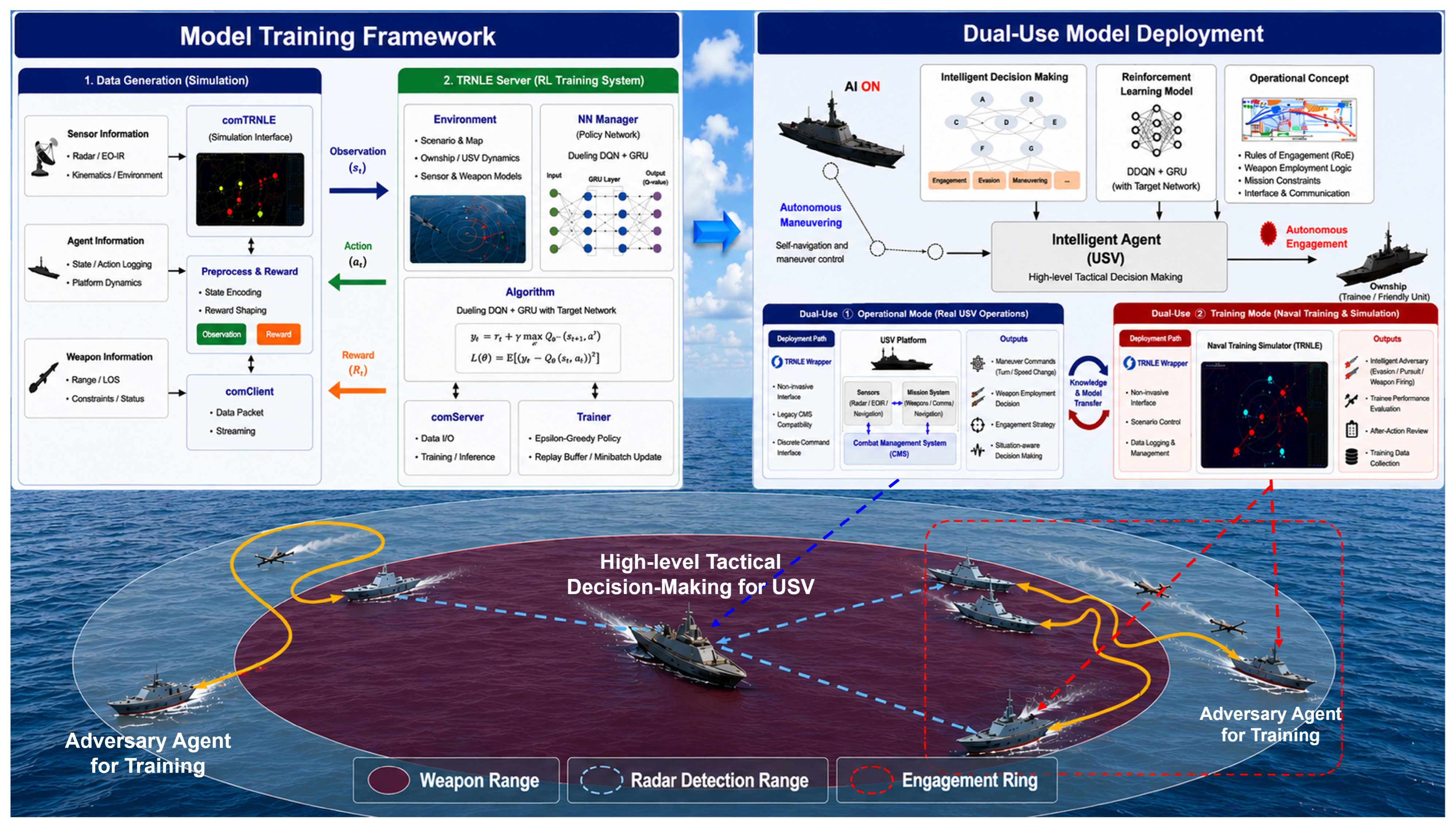
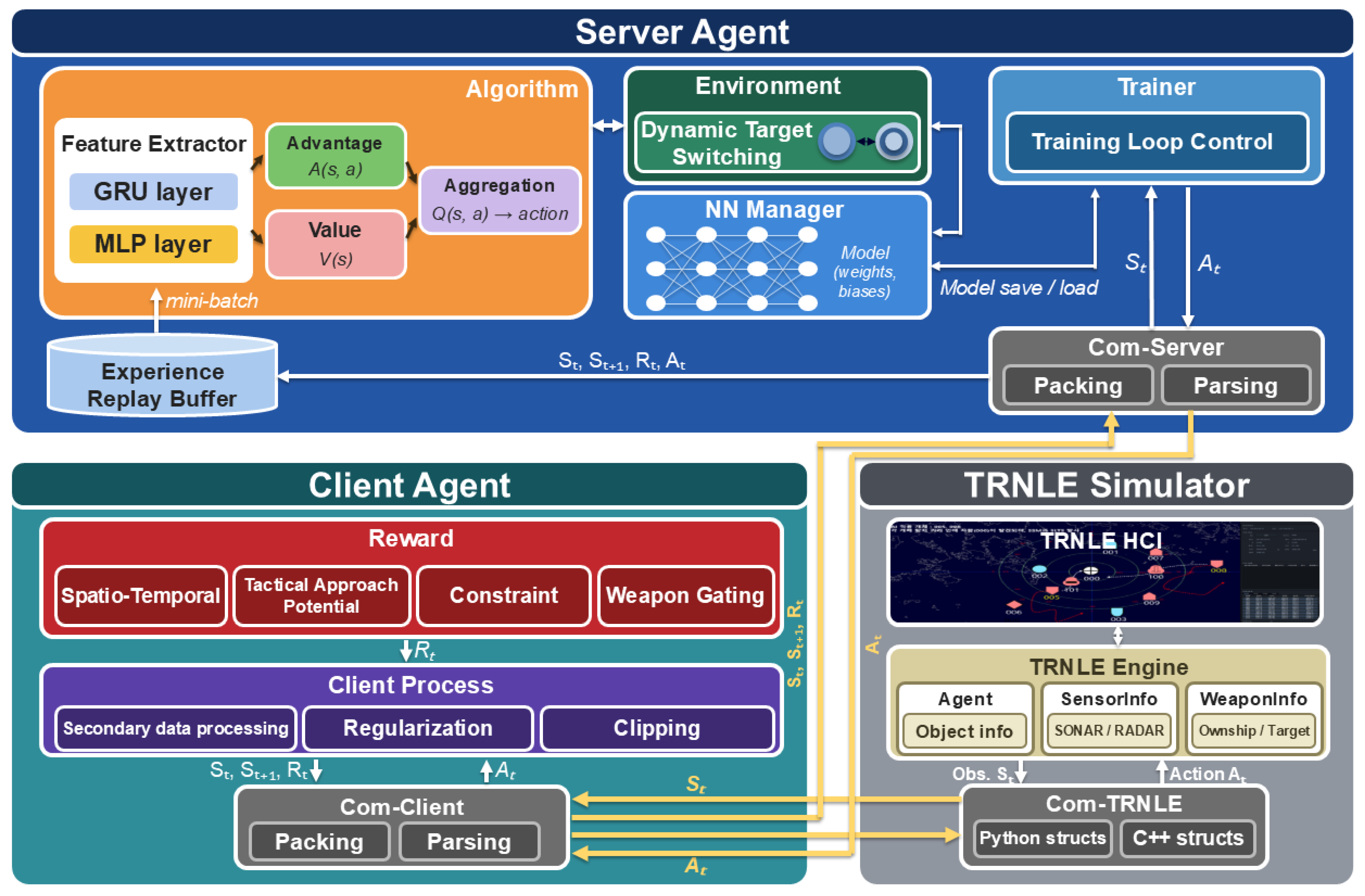
Tactical Maneuver Generation (TMG) determines a vessel’s trajectory and posture to secure survivability and tactical superiority. Traditionally, simulations relied on fixed scripts or simplistic rule-based systems, resulting in monotonic and predictable adversary behaviors, whereas deep reinforcement learning now enables adaptive threat behaviors. In naval doctrine, TMG accelerates the Observe-Orient-Decide-Act (OODA) loop, where providing adaptive threats is essential to challenge a trainee’s decision-making speed and accuracy under stress. In tactical terms, optimizing the Aspect Angle and maintaining optimal engagement ranges are fundamental for maximizing offensive potential while minimizing vulnerability to counter-detection and incoming threats [51]. Such capabilities facilitate the mastery of positional advantage, a core principle in modern naval warfare. These technologies are indispensable not only for OBTS but also for the design and validation of autonomous engagement algorithms for current and next-generation USVs operating in contested maritime environments, where the kinematic, sensor, and engagement-rule constraints apply across training simulator and operational platform alike. An overview of the proposed TAP-DDQN framework is shown in Figure 1.

3.2. Scenario and Tactical Geometry

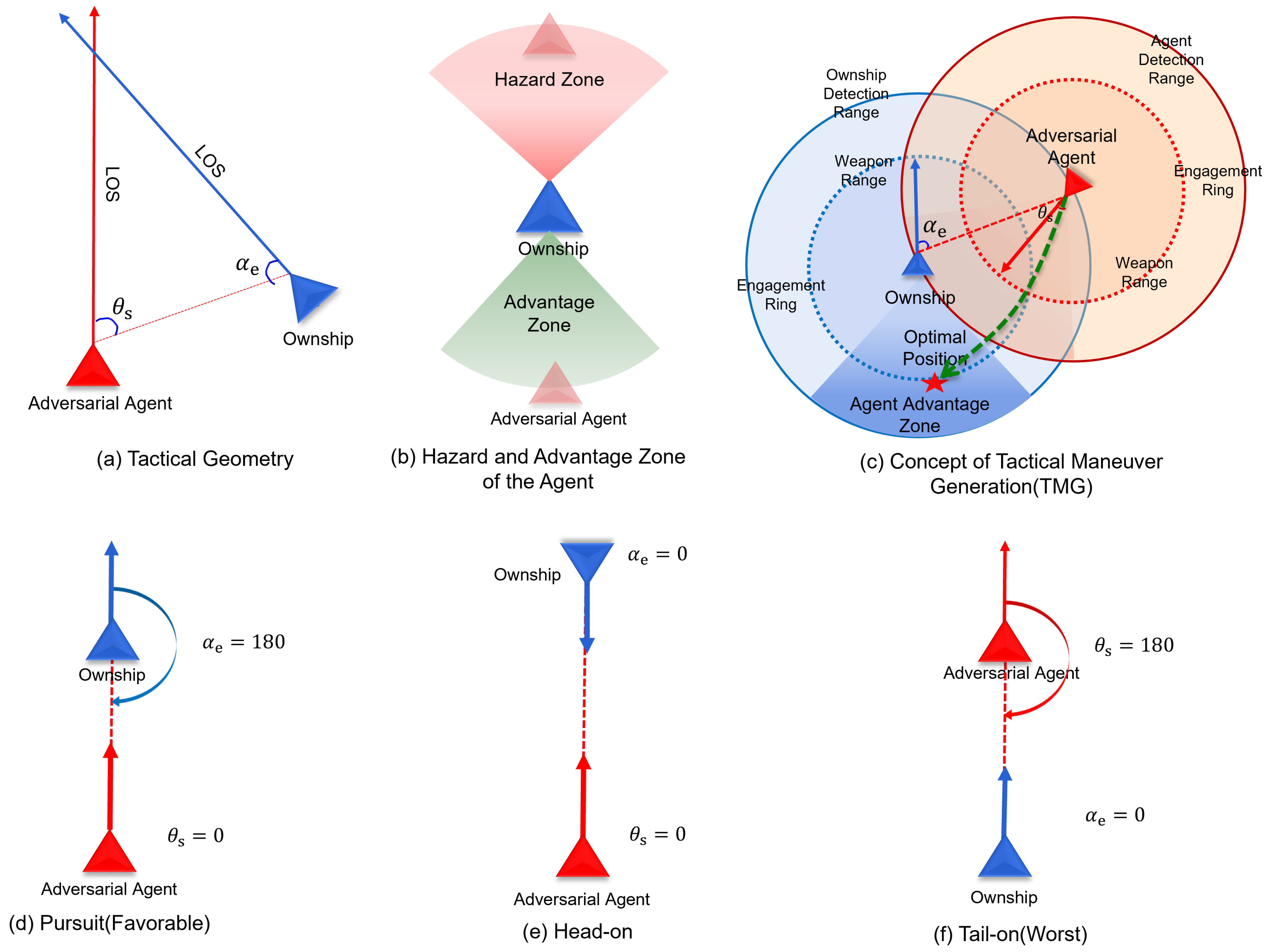
The experimental scenario instantiates a 1-vs-1 surface-ship engagement in an open sea environment. In this scenario, the adversarial agent (USV) maneuvers around the ownship, fires weapons at tactically appropriate moments, and performs evasive maneuvers to stay clear of the ownship’s weapon range. The interaction is bounded by two concentric rings centered on each vessel: a radar detection ring (the outer boundary within which the opposing vessel becomes observable) and a weapon engagement ring (the inner boundary within which a weapon launch is effective), as shown in Figure 2c. The agent engages the ownship only when the ownship enters its own detection range, and the reward shaping described below is tied to the agent’s geometric relationship with these rings.

3.3. Observation and Action

The agent’s state at time t is a 31-dimensional vector that concatenates four semantically distinct sub-states and the most recent action:

$$s_t=\left[s_{\mathrm{agent},t},s_{\mathrm{ownship},t},s_{\mathrm{weapon},t},a_{t-1}\right].$$

(11)

Equations (12)–(14) list the semantic observation variables; the network input applies the encoding detailed in

Table 1. Observation parameters with the per-variable network-input dimension.

Category	Observation	Description	Dim
Agent	$H_t$	Agent health (durability)	1
	$c_t$	Agent course angle	1
	$v_t$	Agent speed	1
	$e_t$	Incoming-projectile presence	2
	$d_t$	Distance error to ownship	1
	$\Delta d_t$	Closing speed	1
	${\Delta }^2{d}_t$	Closing acceleration	1
	$g_t$	Target-distance direction	2
	$b_t$	Remaining weapons	1
	$i_t$	Launch availability/firable step	2
Ownship	$\Delta x_{e_t}$	Relative position X (ownship − agent)	1
	$\Delta y_{e_t}$	Relative position Y (ownship − agent)	1
	$c_{e_t}$	Ownship course	1
	$v_{e_t}$	Ownship velocity	1
	$d_{e_t}$	Agent–ownship distance	1
	${\beta }_{e_t}$	Bearing from ownship to agent	1
	${\theta }_{s_t}$	Relative bearing	1
	$l{r}_{e_t}$	Bearing-quadrant indicator (one-hot)	2
Weapon	$d_{\mathrm{cal}}$	Orthogonal distance to incoming projectile	1
	$\Delta d_{\mathrm{cal}}$	First derivative of orthogonal distance	1
	${\Delta }^2{d}_{\mathrm{cal}}$	Second derivative of orthogonal distance	1
History	$a_{t-1}$	Previous action	6
Total			31

, in which binary indicator variables (incoming-projectile presence, target-distance direction, firable step, and the bearing-quadrant indicator) are one-hot encoded as two dimensions each and the previous action $a_{t-1}$ is one-hot encoded over the six discrete actions.

Agent State (${\mathit{s}}_{\mathit{agent},\mathit{t}}$): The individual variables are summarized in Table 1; the semantic role of each sub-state is as follows. The agent sub-state captures the agent’s own kinematic and armament status, including durability, course, speed, the incoming-projectile presence flag, the distance error to the ownship with its first and second temporal derivatives, the target-distance direction indicator, remaining weapons, and the launch-availability flag:

$$s_{\mathrm{agent},t}=\left[H_t,c_t,v_t,e_t,d_t,\Delta d_t,{\Delta }^2{d}_t,g_t,b_t,i_t\right].$$

(12)

Ownship State (${\mathit{s}}_{\mathit{ownship},\mathit{t}}$): The ownship state encodes the tactical geometry observed from the agent’s perspective, including the relative position components, course, velocity, agent–ownship distance, bearing, relative bearing ${\theta }_{s_t}$, and the discretized bearing-quadrant indicator $l{r}_{e_t}$:

$$s_{\mathrm{ownship},t}=\left[\Delta x_{e_t},\Delta y_{e_t},c_{e_t},v_{e_t},d_{e_t},{\beta }_{e_t},{\theta }_{s_t},l{r}_{e_t}\right].$$

(13)

Weapon State (${\mathit{s}}_{\mathit{weapon},\mathit{t}}$): The weapon sub-state captures the threat posed by any incoming projectile through the orthogonal distance between the projectile’s trajectory line and the agent, together with its first and second temporal derivatives:

$$s_{\mathrm{weapon},t}=\left[d_{\mathrm{cal},t},\Delta d_{\mathrm{cal},t},{\Delta }^2{d}_{\mathrm{cal},t}\right].$$

(14)

Given the projectile trajectory line $ax+by+c=0$ with $a=-\tan \left({\theta }_{\mathrm{proj}\_\mathrm{c}}\right)$ and $b=1$, the orthogonal distance is computed as

$$d_{\mathrm{ortho},t}={\displaystyle \frac{|a{x}_t+b{y}_t+c|}{\sqrt{a^2+b^2}}}.$$

(15)

Action History (${\mathit{a}}_{\mathit{t}-\mathbf{1}}$): The previous action $a_{t-1}$ is appended to provide short-term temporal contexts at the policy-input level, stabilizing action-sequence continuity across 6 decision steps and complementing the latent recurrent representation maintained by the GRU encoder.

Data preprocessing: Every continuous observation variable is preprocessed by per-variable min–max normalization: the raw value is first clipped to a fixed physical range $[v_{\min },v_{\max }]$ and then linearly rescaled to $[0,1]$ via $x\leftarrow (\mathrm{clip}(x,v_{\min },v_{\max })-v_{\min })/(v_{\max }-v_{\min })$. The per-variable ranges are health $[0,400]$, course and bearing $[0°,360°]$, speed $[0,v_{\max }]$, relative distance and target-distance error [0, 100,000]$\mathrm{m}$, the ownship relative bearing ${\theta }_s\in [0°,180°]$, and the first and second temporal derivatives of the target-distance error $[-50,50]$ and $[-1,1]$; the binary status flags and the previous action are one-hot encoded rather than rescaled. Because every observation passes through the same environment normalization routine in both phases, the identical preprocessing is applied during training and inference, so no train–inference distribution shift is introduced.

Action space($\mathcal{A}$): The agent selects among six discrete tactical actions listed in

Table 2. Action types and their functional descriptions.

Action Types	Description
No operation	Maintain current maneuvering
Acceleration	Increase speed by $3\mathrm{m}/{\mathrm{s}}^2$
Deceleration	Decrease speed by $3\mathrm{m}/{\mathrm{s}}^2$
Turn left	Decrease course by $4°$
Turn right	Increase course by $4°$
Weapon firing	Fire a weapon at the ownship

:

$$\mathcal{A}=\{a_{\mathrm{idle}},a_{\mathrm{acc}},a_{\mathrm{dec}},a_{\mathrm{left}},a_{\mathrm{right}},a_{\mathrm{fire}}\}.$$

(16)

Acceleration and deceleration modify the agent’s speed by $\pm 3\mathrm{m}/{\mathrm{s}}^2$, left and right turns change the heading by $\pm 4°$ per step, and $a_{\mathrm{fire}}$ launches a weapon toward the ownship. The no-operation action preserves the current state. This compact discrete action set is directly compatible with the legacy combat management system interface, which enforces deterministic command dispatch.

3.4. Reward Design with a Multiplicative Tactical Approach Potential

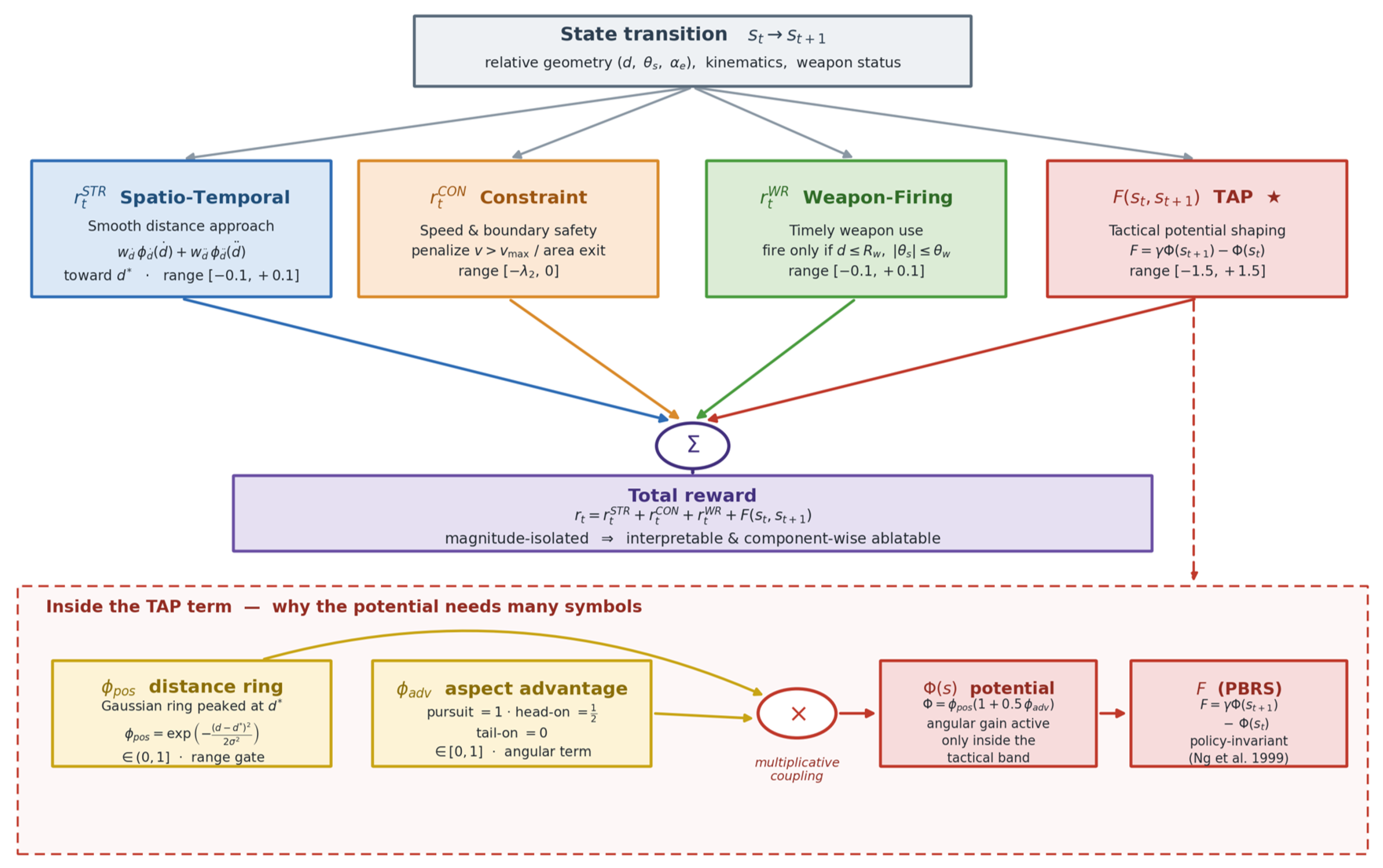
In the TRNLE naval training scenario, the policy must simultaneously maintain tactically advantageous positions, respect physical operational constraints, and launch weapons under appropriate conditions. To make these competing objectives individually interpretable and independently ablatable, the total reward at each time step is decomposed into four semantically distinct components for explainability of the model:

$$r_t=r_t^{\mathrm{STR}}+r_t^{\mathrm{CON}}+r_t^{\mathrm{WR}}+F(s_t,s_{t+1}),$$

(17)

where $r_t^{\mathrm{STR}}$ is the spatio-temporal reward that shapes distance-approach dynamics, $r_t^{\mathrm{CON}}$ is the constraint reward that enforces physical and tactical boundary conditions, $r_t^{\mathrm{WR}}$ is the weapon-firing reward that governs valid ammunition employment, and $F(s_t,s_{t+1})$ is the tactical potential shaping term derived from the Tactical Approach Potential (TAP), which is the principal methodological contribution of this paper.

Table 3. Summary of the four reward components.

Component	Symbol	Weight	Range	Primary Role
Spatio-Temporal	$r_t^{\mathrm{STR}}$	$w_{\dot{d}},w_{\ddot{d}}$	$[-0.1,+0.1]$	Smooth distance approach
Constraint	$r_t^{\mathrm{CON}}$	${\lambda }_1,{\lambda }_2$	$[-{\lambda }_2,0]$	Speed & boundary safety
Weapon-Firing	$r_t^{\mathrm{WR}}$	–	$[-0.1,+0.1]$	Timely weapon use
Tactical Potential	$F(s_t,s_{t+1})$	$w_{\mathrm{ang}}=0.5$	$[-1.5,+1.5]$	Aspect & range advantage

summarizes the weight and range of the four components, and Figure 3 provides a schematic overview of how each sub-reward contributes to the total; each is detailed in the following subsections.

3.4.1. Spatio-Temporal Reward (STR)

The STR guides the agent toward the tactically optimal engagement distance $d^{*}$ by rewarding smooth approach maneuvers and penalizing excessive movement. Unlike a proportional distance reward, STR integrates the first and second temporal derivatives of the relative distance, enabling the agent to learn not only where to be but how to move there over time. Let $d_t$ denote the relative distance between the agent and the ownship at time t, ${\dot{d}}_{\mathrm{cal}}$ the closing rate, and ${\ddot{d}}_t$ the relative acceleration. The STR is defined as:

$$r_t^{\mathrm{STR}}=w_{\dot{d}}·{\varphi }_{\dot{d}}\left({\dot{d}}_{\mathrm{cal}}\right)+w_{\ddot{d}}·{\varphi }_{\ddot{d}}\left({\ddot{d}}_t\right),$$

(18)

where the two sub-terms are:

$${\varphi }_{\dot{d}}\left({\dot{d}}_{\mathrm{cal}}\right)=\left\{\begin{array}{cc}+0.1,\hfill & {\dot{d}}_{\mathrm{cal}}<0\left(\mathrm{closing}\mathrm{toward}{d}^{*}\right)\hfill \\ -0.1,\hfill & {\dot{d}}_{\mathrm{cal}}>0\left(\mathrm{receding}\mathrm{from}{d}^{*}\right)\hfill \\ 0,\hfill & \mathrm{otherwise}\hfill \end{array}\right.$$

(19)

$${\varphi }_{\ddot{d}}\left({\ddot{d}}_t\right)=\left\{\begin{array}{cc}0.1·{\ddot{d}}_t,\hfill & {\ddot{d}}_t<-\zeta \left(\mathrm{smooth}\mathrm{deceleration}\right)\hfill \\ -0.1·{\ddot{d}}_t,\hfill & 0<{\ddot{d}}_t<\kappa \left(\mathrm{penalize}\mathrm{acceleration}\mathrm{away}\right)\hfill \\ 0,\hfill & \mathrm{otherwise}\hfill \end{array}\right.$$

(20)

Here, ${\varphi }_{\dot{d}}$ term rewards closing behavior and penalizes diverging behavior, while ${\varphi }_{\ddot{d}}$ rewards controlled deceleration and penalizes abrupt acceleration away from the target zone.

3.4.2. Constraint Reward

The constraint reward enforces physical and operational boundary conditions that must not be violated during tactical maneuvering. These constraints capture safety and realism requirements that cannot be adequately expressed as shaped potential gradients: excessively low speeds and unnecessary acceleration at high-speed. Let $v_t$ be the agent’s own speed and $a_t\in \{0,1\}$ be the acceleration action (1 = maximum thrust). The constraint reward is defined as:

$$r_t^{\mathrm{CON}}=\left\{\begin{array}{cc}-{\lambda }_1,\hfill & v_t<v_{\min }\hfill \\ -{\lambda }_2,\hfill & v_t\ge v_{\max }\wedge a_t=1\hfill \\ 0,\hfill & \mathrm{otherwise},\hfill \end{array}\right.$$

(21)

where $v_{\min }=20\mathrm{km}/\mathrm{h}$, $v_{\max }=50\mathrm{km}/\mathrm{h}$, ${\lambda }_1>0$, and ${\lambda }_2>0$ are penalty magnitudes.

The first condition penalizes near-stall speeds that would render the vessel vulnerable in real engagements; the second penalizes full acceleration when the vessel is already at high speed, preventing the agent from exploiting high-speed dashing as a reward-hacking strategy. Because movement and weapon-firing decisions are produced by the policy, isolating the speed constraint into a dedicated component provides a clean credit-assignment signal and cannot be masked by the STR gradient.

3.4.3. Weapon-Firing Reward

In environments where weapon firing yields a positive reward, an unconstrained agent will launch weapons continuously to maximize immediate gains. To prevent premature or excessive firing, a binary gating variable $\text{weapon\_able\_step}\in \{0,1\}$ indicates whether weapon employment is tactically permissible at time t. Let $f_t\in \{0,1\}$ denote a firing event ($f_t=1$ = firing action); the weapon-firing reward is formulated as:    

$$r_t^{\mathrm{WR}}=\left\{\begin{array}{cc}+0.1,\hfill & \text{weapon\_able\_step}=1\wedge f_t=1,\hfill \\ -0.1,\hfill & \text{weapon\_able\_step}=0\wedge f_t=1,\hfill \\ 0,\hfill & \mathrm{otherwise}.\hfill \end{array}\right.$$

(22)

Firing within a permitted step yields a positive reward, while unauthorized or excessive firing is penalized. Because the weapon-firing and spatio-temporal rewards are mutually exclusive at each step, the agent must strategically balance maneuvering and weapon engagement rather than maximizing one at the expense of the other.

3.4.4. Tactical Approach Potential (TAP)

To overcome the sparse-reward challenge and encode tactical domain knowledge giving dense feedback, a potential-based shaping term [17] preserves the set of optimal policies of the original reward provided that the underlying potential is bounded and depends only on the state. Let $\mathrm{\Phi }\left(s\right)$ be the Tactical Approach Potential encoding both spatial proximity to the designated engagement distance and the angular tactical advantage of the adversarial agent relative to the ownship. The shaping reward is

$$F(s_t,s_{t+1})=\gamma \mathrm{\Phi }(s_{t+1};d_{t+1}^{*})-\mathrm{\Phi }(s_t;d_t^{*}),$$

(23)

where $0\le \gamma <1$ is the discount factor and $d_t^{*}$ denotes the engagement target active when $s_t$ was collected; when the target is held fixed, Equation (23) reduces to the static form of Ng et al. [17]. By the shaping theorem [17], augmenting the original reward as $r_t^{\prime }=r_t+F(s_t,s_{t+1})$ does not change the optimal policy, provided $\mathrm{\Phi }\left(s\right)$ is a bounded and state-only potential. The $\mathrm{\Phi }\left(s\right)$ is decomposed into a distance-based term ${\varphi }_{\mathrm{pos}}$ and an aspect-aware term ${\varphi }_{\mathrm{adv}}$, combined multiplicatively:

$$\mathrm{\Phi }\left(s\right)={\varphi }_{\mathrm{pos}}\left(s\right)·\left(1+w_{\mathrm{ang}}{\varphi }_{\mathrm{adv}}\left(s\right)\right),$$

(24)

where $w_{\mathrm{ang}}=0.5$ balances range and aspect objectives. This value is chosen so that the tactical multiplier $(1+w_{\mathrm{ang}}{\varphi }_{\mathrm{adv}})\in [1,1.5]$ for ${\varphi }_{\mathrm{adv}}\in [0,1]$, which bounds the potential to $\mathrm{\Phi }\in (0,1.5]$ while still allowing the aspect term to modulate the distance signal by up to $50\%$. Because the potential varies continuously with $w_{\mathrm{ang}}$, moderate deviations from this value rescale the strength of the aspect modulation without altering the structure of the shaping term: larger values would allow the aspect term to override range regulation, whereas smaller values would render the angular guidance negligible.

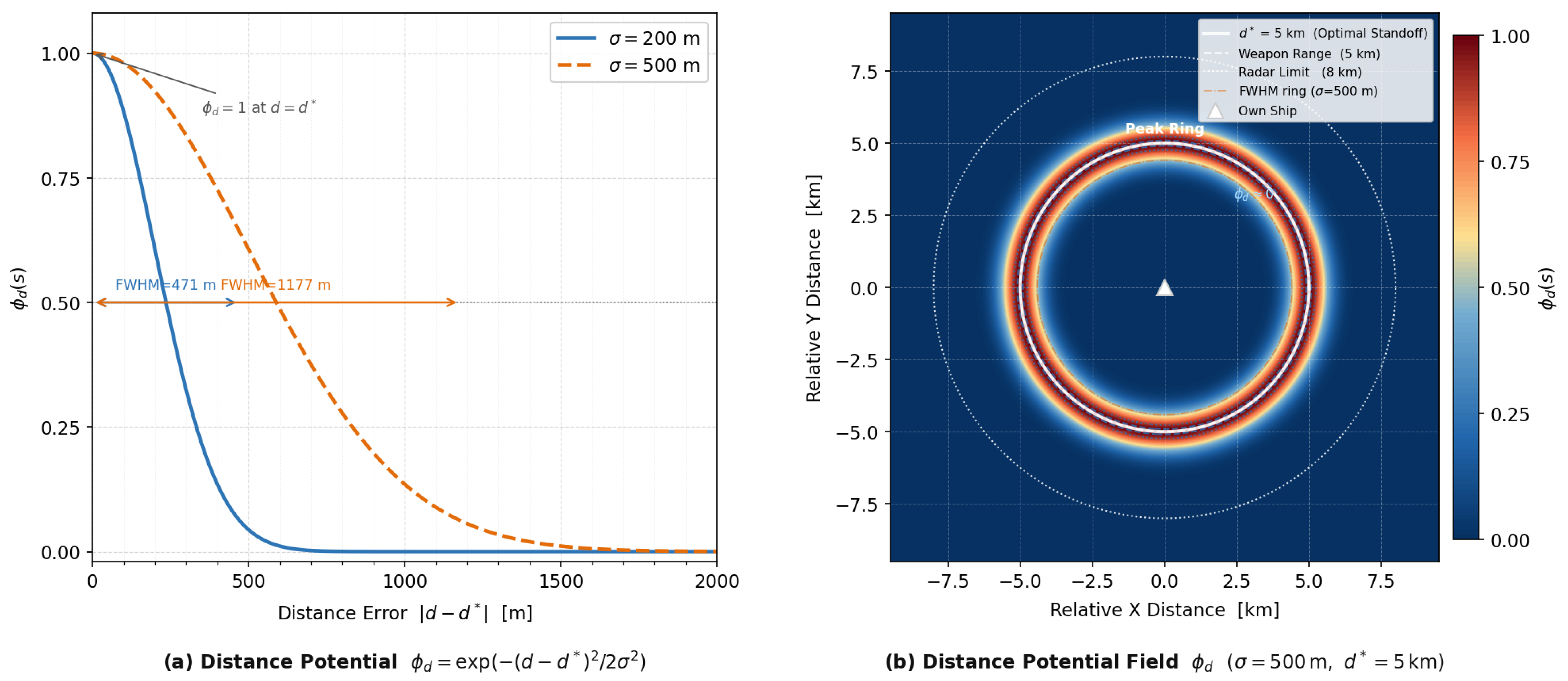
The distance component is modeled as a Gaussian envelope centered on the designated engagement distance $d^{*}$:

$${\varphi }_{\mathrm{pos}}\left(s\right)=\exp \left(-{\displaystyle \frac{{\left(d\left(s\right)-d^{*}\right)}^2}{2{\sigma }^2}}\right),$$

(25)

where $d\left(s\right)$ is the current relative distance, $d^{*}$ is the designated engagement distance, which is assigned dynamically by the Dynamic Target Curriculum (Section 3.5), and $\sigma$ controls the ring width. ${\varphi }_{\mathrm{pos}}\in [0,1]$, reaching its maximum only when $d\left(s\right)=d^{*}$. The fixed value $\sigma =500\mathrm{m}$ is applied throughout training, and the dynamic assignment of $d^{*}$ is explained in Section 3.5. The resulting distance potential is illustrated in Figure 4.

The aspect component is derived from the relative tactical geometry between agent and ownship. Let

$${\theta }_s=\left|\mathrm{normalize}\left({\beta }_{e\to o}-{\psi }_e\right)\right|\in [0°,180°],$$

(26)

be the enemy aspect angle, the angle from the enemy ship’s heading to the ownship, where ${\beta }_{e\to o}=({\beta }_{o\to e}+180°)\mathrm{mod}360°$ is the reverse bearing from enemy to ownship, and ${\psi }_e$ is the enemy’s compass heading. Let ${\alpha }_e=|{\beta }_{o\to e}-{\psi }_o|\in [0°,180°]$ be the ownship’s relative bearing to the enemy. The aspect-aware advantage potential is then:

$${\varphi }_{\mathrm{adv}}\left(s\right)={\displaystyle \frac{\cos {\theta }_s-\cos {\alpha }_e+2}{4}}\in [0,+1].$$

(27)

(${\varphi }_{\mathrm{adv}}\approx +1$) corresponds to the pursuit posture (${\theta }_s\approx 0°$, ${\alpha }_e\approx 180°$), where the agent heads directly toward the ownship while approaching from its stern—the most tactically advantageous configuration. Conversely, ${\varphi }_{\mathrm{adv}}\approx 0$ denotes the tail-on posture (${\theta }_s\approx 180°$, ${\alpha }_e\approx 0°$), where the agent’s stern is exposed to the ownship.

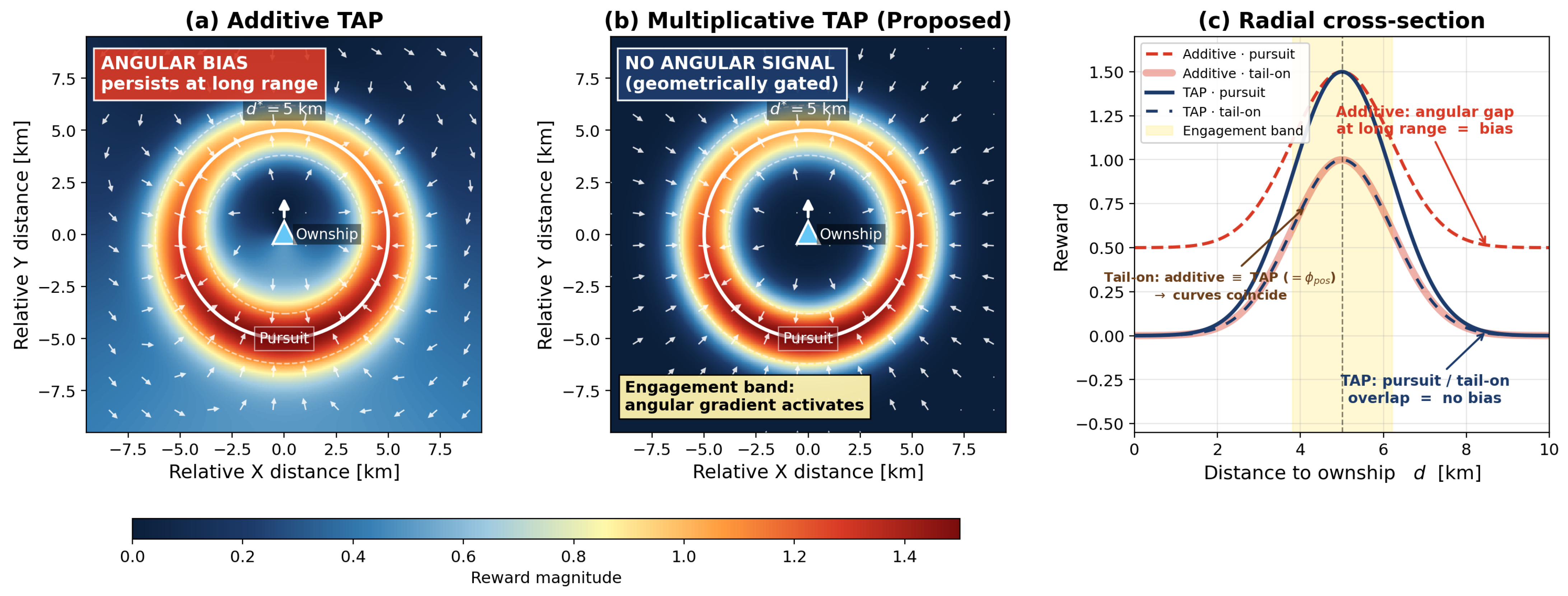
The multiplicative form is what makes TAP behave differently from the additive shaping schemes as shown in Figure 5 [47,48]. Multiplying ${\varphi }_{\mathrm{adv}}$ by ${\varphi }_{\mathrm{pos}}$ couples the angular term to distance. When the agent is far from the ring, ${\varphi }_{\mathrm{pos}}$ is near zero, so the angular term contributes nothing. That is, the policy is not pulled toward a particular heading until it has approached the ring. When the agent is on the ring, ${\varphi }_{\mathrm{pos}}$ is one and the angular term is active. The multiplier (1 + 0.5 ${\varphi }_{\mathrm{adv}}$) ranges over [1, 1.5]. As shown in Figure 2d, pursuit (best aspect) case gives 1.5. In contrast, as shown in Figure 2f, tail-on (worst aspect) case gives 1.0 and preserves the distance-ring reward unchanged.

Although the PBRS theorem of Ng et al. [17] guarantees that any potential-based shaping preserves the optimal policy, this guarantee applies only when the potential function satisfies two conditions: it must depend on the current state alone, and it must be bounded across the state space. Because ${\varphi }_{\mathrm{adv}}$ encodes angular geometry, we confirm both conditions explicitly for the TAP potential of Equation (24).

Regarding state-only dependence, both sub-components are determined entirely by the configuration at state s: ${\varphi }_{\mathrm{pos}}\left(s\right)$ depends only on the inter-vessel distance $d\left(s\right)$, and ${\varphi }_{\mathrm{adv}}\left(s\right)$ on the angles ${\theta }_s\left(s\right)$ and ${\alpha }_e\left(s\right)$, all of which are observable geometric quantities fixed at time t. The action $a_t\in \mathcal{A}$ influences the next state $s_{t+1}$ through the environment dynamics, but leaves $\mathrm{\Phi }\left(s_t\right)$ unchanged. Hence $\mathrm{\Phi }$ is a pure state function.

Regarding boundedness, since the exponent in Equation (25) is non-positive, ${\varphi }_{\mathrm{pos}}\left(s\right)\in (0,1]$ for all s. From Equation (25), the tactical multiplier satisfies $(1+0.5{\varphi }_{\mathrm{adv}})\in [1,1.5]$. Combining these ranges gives:

$$\mathrm{\Phi }\left(s\right)=\underset{\in (0,1]}{\underbrace{{\varphi }_{\mathrm{pos}}\left(s\right)}}·\underset{\in [1,1.5]}{\underbrace{\left(1+0.5{\varphi }_{\mathrm{adv}}\left(s\right)\right)}}\in (0,1.5]\forall s\in \mathcal{S}.$$

(28)

The potential is therefore strictly positive and bounded above by $1.5$ on the entire state space, satisfying the boundedness condition. Note that the multiplier never reaches zero: even at the tactically worst posture (${\varphi }_{\mathrm{adv}}=0$), the multiplier equals 1, so the agent always receives a non-zero distance-ring reward; the aspect advantage modulates this base reward by up to $50\%$ at the optimal pursuit heading.

With both conditions verified, the optimality structure under the reward $r_t^{\prime }=r_t+F(s_t,s_{t+1})$ can be derived through the Bellman fixed-point argument. Assuming $Q^{\prime *}(s,a)=Q^{*}(s,a)-\mathrm{\Phi }\left(s\right)$ and substituting into the shaped Bellman optimality equation yields:

$$\begin{array}{cc}\hfill Q^{\prime *}(s,a)& ={\mathbb{E}}_{s^{\prime }}\left[r(s,a,s^{\prime })+\gamma \mathrm{\Phi }\left(s^{\prime }\right)-\mathrm{\Phi }\left(s\right)+\gamma \underset{a^{\prime }}{\max }{Q}^{\prime *}(s^{\prime },a^{\prime })\right]\hfill \\ \hfill & ={\mathbb{E}}_{s^{\prime }}\left[r(s,a,s^{\prime })+\gamma \mathrm{\Phi }\left(s^{\prime }\right)-\mathrm{\Phi }\left(s\right)+\gamma \left(V^{*}\left(s^{\prime }\right)-\mathrm{\Phi }\left(s^{\prime }\right)\right)\right]\hfill \\ \hfill & =\underset{=Q^{*}(s,a)}{\underbrace{{\mathbb{E}}_{s^{\prime }}\left[r(s,a,s^{\prime })+\gamma V^{*}\left(s^{\prime }\right)\right]}}-\mathrm{\Phi }\left(s\right).\hfill \end{array}$$

(29)

Since the shaped Bellman operator is a $\gamma$-contraction on the space of bounded functions, $Q^{\prime *}(s,a)=Q^{*}(s,a)-\mathrm{\Phi }\left(s\right)$ is its unique fixed point. Because $\mathrm{\Phi }\left(s\right)$ is subtracted equally from $Q^{*}(s,a)$ for every action, it does not affect the ranking of actions at any state, and the optimal policy is therefore identical under both the original and shaped rewards:

$${\pi }^{\prime *}\left(s\right)={\arg \max }_a{Q}^{\prime *}(s,a)={\arg \max }_a\left[Q^{*}(s,a)-\mathrm{\Phi }\left(s\right)\right]={\arg \max }_a{Q}^{*}(s,a)={\pi }^{*}\left(s\right).$$

(30)

A further consequence is that the one-step temporal-difference (TD) error ${\delta }_t=r_t+\gamma V^{*}\left(s_{t+1}\right)-Q^{*}(s_t,a_t)$ is also unchanged by the shaping term, since the four contributions $+\gamma \mathrm{\Phi }\left(s_{t+1}\right)$, $-\mathrm{\Phi }\left(s_t\right)$, $-\gamma \mathrm{\Phi }\left(s_{t+1}\right)$, and $+\mathrm{\Phi }\left(s_t\right)$ cancel completely in the shaped TD error ${\delta }_t^{\prime }$:

$${\delta }_t^{\prime }=r_t^{\prime }+\gamma V^{\prime *}\left(s_{t+1}\right)-Q^{\prime *}(s_t,a_t)=r_t+\gamma V^{*}\left(s_{t+1}\right)-Q^{*}(s_t,a_t)={\delta }_t.$$

(31)

This cancellation shows that, under the stated assumptions, the shaping term leaves the optimal action-value ordering, and hence the optimal policy unchanged. We emphasize that this establishes optimal-policy invariance only; it does not by itself guarantee that transient TD errors, optimization trajectories, convergence speed, or stability under neural-network function approximation are unchanged. Any observed improvement in convergence speed or stability is therefore attributed to the experimental evidence reported below, rather than inferred from this value transformation.

The distance potential ${\varphi }_{\mathrm{pos}}$ is centered on the desired engagement distance $d^{*}$, which the Dynamic Target Curriculum of Section 3.5 switches between the weapon range $R_w$ and the detection range $R_d$ during training, so the potential is time-varying through $d^{*}$. We therefore invoke the dynamic potential-based shaping result of Devlin and Kudenko [46]: policy invariance is preserved for a time-varying potential provided the shaping reward retains the difference form $F_t=\gamma \mathrm{\Phi }(s_{t+1};d_{t+1}^{*})-\mathrm{\Phi }(s_t;d_t^{*})$, which our shaping term satisfies. Between consecutive switches the target is fixed, so the static guarantee of Ng et al. [17] applies segment-wise and the perturbation induced at each switch is bounded. The shaping term is computed online at collection time using the active $d^{*}$ and is added to the reward before storage (Algorithm 1); the replay buffer therefore retains only $(s_t,a_t,r_t,s_{t+1})$, so $d^{*}$ itself is not stored and F is never recomputed during training. The spatial distributions of ${\varphi }_{\mathrm{pos}}$, ${\varphi }_{\mathrm{adv}}$, and $\mathrm{\Phi }\left(s\right)$ are illustrated in Figure 4. The training procedure is summarized in Algorithm 1.

Algorithm 1 TAP-DDQN training with Tactical Approach Potential shaping and Dynamic Target Curriculum

1: Initialize policy ${\pi }_{\theta }$, target network ${\widehat{Q}}_{\psi }$, replay buffer $\mathcal{D}$   2: Initialize TAP parameters: ring width $\sigma$, aspect weight $w_{\mathrm{ang}}$   3: Initialize curriculum target $d^{*}\leftarrow R_w$, dwell counter $c\leftarrow 0$, goal tolerance ${\delta }_{\mathrm{goal}}$, dwell steps $N_{\mathrm{stay}}$   4: Initialize constraint thresholds $v_{\min }$, $v_{\max }$, ${\lambda }_1$, ${\lambda }_2$   5: for each episode do   6:       Reset environment; receive initial state $s_0$; $d^{*}\leftarrow R_w$; $c\leftarrow 0$   7:       for each timestep t do   8:             Select action $a_t\sim {\pi }_{\theta }\left(s_t\right)$ ($\epsilon$-greedy)   9:             Execute $a_t$; observe $s_{t+1}$, event flags $e_t$ 10:             $d_t^{*}\leftarrow d^{*}$ 11:             if $|d_t-d^{*}|\le {\delta }_{\mathrm{goal}}$ then 12:                  $c\leftarrow c+1$ 13:                  if $c\ge N_{\mathrm{stay}}$ then 14:                        $d^{*}\leftarrow R_w+R_d-d^{*}$; $c\leftarrow 0$ 15:                  end if 16:             else 17:                  $c\leftarrow 0$ 18:             end if 19:             $d_{t+1}^{*}\leftarrow d^{*}$ 20:             $r_t^{\mathrm{STR}}\leftarrow w_{\dot{d}}{\varphi }_{\dot{d}}\left({\dot{d}}_{\mathrm{cal}}\right)+w_{\ddot{d}}{\varphi }_{\ddot{d}}\left({\ddot{d}}_t\right)$                             (Equation (18)) 21:             $r_t^{\mathrm{CON}}\leftarrow \mathrm{constraint}\mathrm{penalty}(v_t,a_t)$                          (Equation (21)) 22:             $r_t^{\mathrm{WR}}\leftarrow \mathrm{weapon}\mathrm{reward}(f_t,\text{weapon\_able\_step})$                     (Equation (22)) 23:             $F_t\leftarrow \gamma \mathrm{\Phi }(s_{t+1};d_{t+1}^{*})-\mathrm{\Phi }(s_t;d_t^{*})$                             (Equation (23)) 24:             $r_t\leftarrow r_t^{\mathrm{STR}}+r_t^{\mathrm{CON}}+r_t^{\mathrm{WR}}+F_t$ 25:             Store $(s_t,a_t,r_t,s_{t+1})$ in $\mathcal{D}$ 26:             Sample mini-batch; update ${\pi }_{\theta }$ via the Dueling DQN loss 27:             Periodically update ${\widehat{Q}}_{\psi }\leftarrow {\pi }_{\theta }$ 28:             $s_t\leftarrow s_{t+1}$ 29:       end for 30: end for

3.5. Curriculum Learning Strategy via Dynamic Target Switching

To further enhance training efficiency and prevent catastrophic forgetting, the proposed framework employs a curriculum learning strategy. In conventional staged curriculum learning, transitions between difficulty levels are fixed by hand, which may cause inconsistent performance and catastrophic forgetting of earlier skills. Moreover, manually designing an appropriate staged curriculum is difficult and time-consuming. To address this, the proposed method employs oscillatory target switching: once the agent achieves the engagement distance $d^{*}$, the target toggles to the opposite range. Concretely, the target set is $d^{*}\in \{R_w,R_d\}$, where $R_w$ is the weapon range and $R_d$ is the radar detection range (

Table 4. Initial conditions and environmental parameters for each entity.

Category	Ownship	Agent
Starting point	Random area (within bounds)	Within detection area
Initial course	Random $\in [0°,360°)$	Random $\in [0°,360°)$
Initial speed	9.7 knots (18 km/h)	Random $\in [0,27]$ knots (≈$[0,50]$ km/h)
Radar detection range ($R_{\mathrm{d}}$)	8 km	8 km
Weapon range ($R_{\mathrm{w}}$)	5 km	5 km
Weapon	Yes	Yes
Action	Course, Velocity, Weapon Firing	Course, Velocity, Weapon Firing

); each episode is initialized at $d^{*}=R_w$ to first learn immediate engagement. The achievement condition is $|d_t-d^{*}|<{\delta }_{\mathrm{goal}}$ with the goal tolerance set to the ring width ${\delta }_{\mathrm{goal}}=\sigma =500\mathrm{m}$; it must be held for $N_{\mathrm{stay}}$ consecutive steps, and it is checked at every step so that the toggle to the opposite range takes effect immediately within the episode.

Because the target index cycles through $\{R_w,R_d,R_w,R_d\}$ and wraps around, multiple switches may occur within a single episode. The potential difference is computed online with the target that is active when each transition is collected, and the resulting shaping term is folded into the reward before storage; the active $d^{*}$ is therefore not stored separately (Algorithm 1). This design enforces repeated boundary-zone learning across the full operational envelope, building a robust policy over both short- and long-range engagements without manual curriculum staging. By dynamically switching between detection-range interior and weapon range exterior, the environment prevents the agent from converging to a single-distance strategy and promotes generalization across diverse tactical phases. This oscillatory switching ensures that the agent is exposed to the full engagement envelope from close weapon range to long detection range including intermediate distances.

In the experimental configuration used in this study, the Gaussian ring width is fixed at $\sigma =500\mathrm{m}$ throughout training, rather than being progressively reduced. Full-envelope coverage is instead achieved entirely through the oscillatory target-switching mechanism described in Section 3.5: once the agent achieves the designated engagement distance, $d^{*}$ is automatically switched between the weapon engagement range (short range) and the sensor detection range (long range), enforcing repeated learning across both tactical distance boundaries. In addition, by enforcing repetitive learning of the boundary areas of maximum and minimum engagement distances, it fosters the formation of a robust policy across the entire operational range.

4. Learning Framework for Intelligent Simulation Target Objects

The simulation TRaiNing Learning Environment (TRNLE) provides the simulation environment and interfaces required for training and inference of intelligent simulation targets within a surface-ship simulation training system. Rather than replacing the existing combat simulator, TRNLE wraps a legacy OBTS software stack and augments it with the machine-learning-specific functions needed for RL-based model training, inference, and performance analysis [52]. Through this non-invasive integration, the sensor models, weapon simulators, and engagement rules used in operational training are exposed to the RL agent without modification of the certified combat management software.

TRNLE Framework

The training framework consists of three modules—the TRNLE environment, a Client Agent, and a Server Agent—as shown in Figure 6 and as summarized in

Table 5. Component description for training.

Module	Class Name	Description
Environment	TRNLE	Data generation and object control for training.
	Com-TRNLE	Data exchange and conversion between TRNLE and Client Agent across platforms.
Client Agent	Agent Mng	Management of training objects by platform.
	Preprocess	Observation data pre-processing.
	Reward	Compute the reward function of Equation (17).
	Com-Client	Send and receive data.
	Sensor Mng	Sensor attribute data of the simulation target.
	Weapon Mng	Weapon attribute data of the simulation target.
Server Agent	Trainer	Manage and control server-agent training settings.
	Com-Server	Send and receive data.
	Algorithm	Management of RL algorithm configuration.
	Neural Network	Manage neural networks for training.
	Environment	Processing of environment information for RL.
	NNModel	Save trained models and weight values.

. Because the simulation environment and the training modules are implemented in different programming languages and run as separate processes, a lightweight TRNLE wrapper handles cross-process data exchange and format conversion. Upon scenario initialization, TRNLE loads the pre-designed scenario configuration, instantiates the corresponding simulation entities, and advances the simulation clock in fixed timesteps. At each step, the Client Agent preprocesses sensor and weapon observations for both the agent and the ownship and computes the four-component reward defined in Section 3.4. Then, it forwards the resulting $(s_t,r_t)$ tuple to the Server Agent. The Server Agent runs the core RL training loop: it consumes the processed experience, updates the neural network parameters via the DDQN objective, selects the next action $a_t$ from the current policy ${\pi }_{\theta }$, and returns the action command to the Client Agent. This exchange persists for the full scenario, and the modular interface permits straightforward incorporation of additional RL algorithms, sensor models, or engagement scenarios without modification of the underlying legacy simulator.

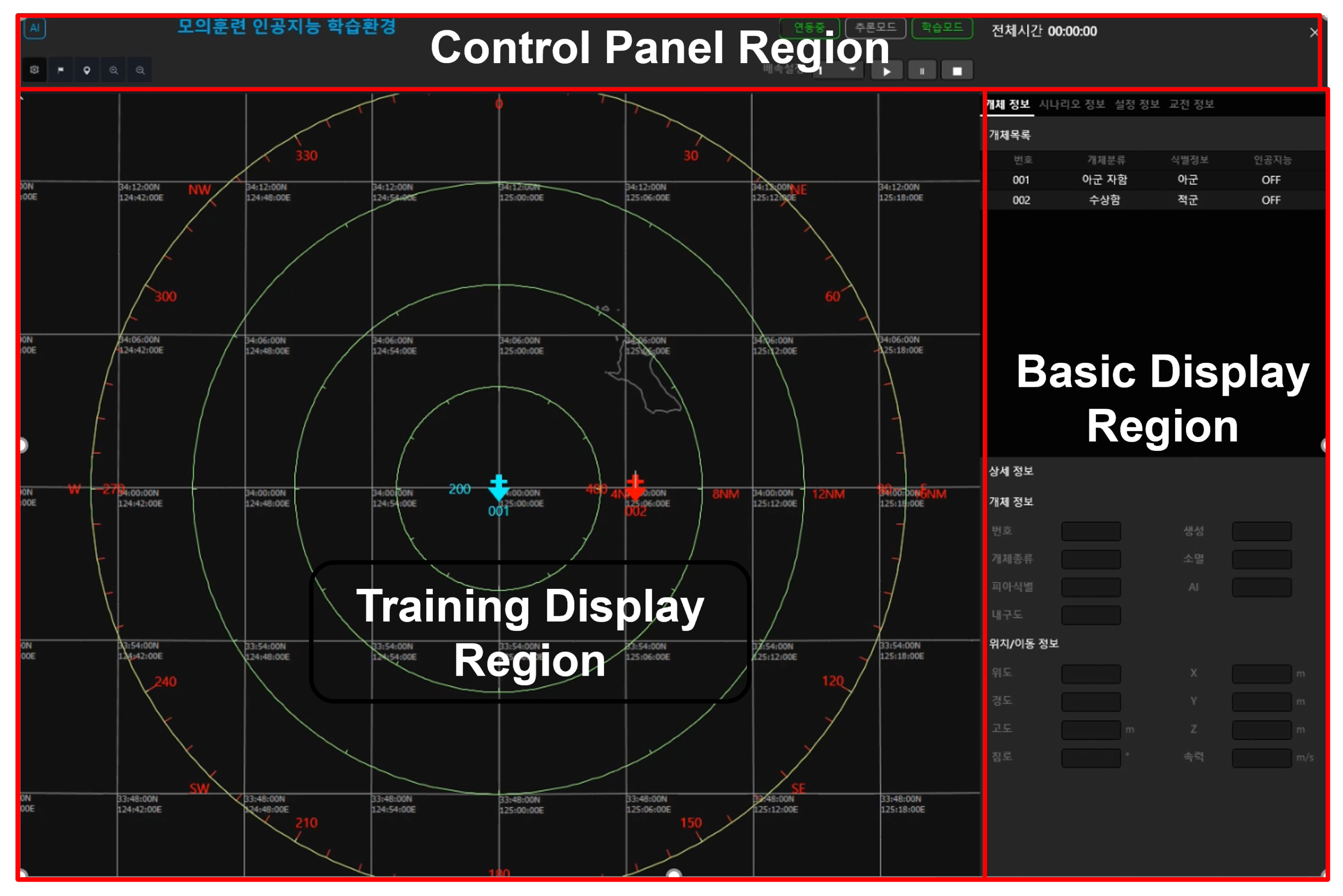
TRNLE operates in two complementary modes. Training mode generates interaction data for RL model updates, supports parallel execution of multiple heterogeneous scenarios to diversify the training distribution, and offers a speed-up option that accelerates data collection. Inference mode provides visual evaluation of a trained model, permits direct operator intervention through a “manual action” control, and also supports time acceleration for efficient validation runs. The TRNLE user interface is divided into a Training Display Region, a Basic Display Region, and a Control Panel Region, as shown in Figure 7.

5. Experiment and Results

5.1. Experimental Setup and Ablation Design

Table 4 summarizes the initial scenario conditions common to all experiments. The ownship is placed randomly within the scenario bounds, while the agent is initialized within the detection envelope; both entities are armed and can command course, velocity, and weapon firing. The intelligent target’s initial position and course are randomized at each episode to diversify the training distribution and prevent bias toward any single spatial configuration. Each episode terminates after 3000 steps.

The ablation study isolates the contribution of three design choices—(i) the TAP multiplicative potential shaping, (ii) the Dynamic Target Curriculum (DTC), and (iii) the GRU recurrent encoder—against common value-based and policy-gradient baselines. All configurations are trained under identical TRNLE conditions, state/action spaces, random seeds, and training budgets (30 M environment steps, three independent seeds per configuration). Hyperparameters are listed in

Table 6. Hyperparameters used for all reinforcement learning configurations.

Parameter	DQN-MLP	Dueling DQN-MLP	Dueling DQN-GRU	PPO-MLP
MLP hidden dim	128	128	–	128
RNN hidden dim	–	–	128	–
Input dimension	31
Output dimension	6
Learning rate ($lr$)	$1\times {10}^{-3}$			Actor: $1\times {10}^{-4}$ Critic: $5\times {10}^{-4}$
Discount factor ($\gamma$)	0.99
Update cycle	50
Episode limit (steps)	3000
Batch size (episodes)	5			10
$\epsilon$ start/min/decay	1.0/0.05/0.99			–
PPO clip/K epochs	–			0.2/10

. For the recurrent configurations, the GRU hidden state is zero-initialized ($h_0=\mathbf{0}$) at the start of every episode and reset at each episode boundary.

The seven configurations comprise six comparative variants (A–F) and the proposed full model (G):

(A) 

Rule-based CGF (Baseline): deterministic rules for maneuvering and firing; lower-bound reference representing the conventional, non-adaptive adversary behavior found in existing OBTS.

(B) 

DQN+MLP w/o TAP: standard DQN with an MLP encoder and STR + constraint + weapon rewards, without TAP shaping or Dueling decomposition.

(C) 

PPO+MLP w/o TAP: policy-gradient counterpart of (B), evaluating whether on-policy methods offer advantages in this discrete-action tactical domain.

(D) 

DDQN+MLP w/o TAP: Dueling DQN with MLP encoder and STR but without TAP shaping.

(E) 

DDQN+MLP w/ TAP (Additive): Variant (D) augmented with the additive TAP shaping. This variant serves as a controlled internal additive surrogate for additive tactical-shaping families [47,48]: it shares identical distance and aspect potentials with the multiplicative variants and differs only in the coupling structure, reproducing the range-independent angular gradient characteristic of additive schemes.

(F) 

DDQN+MLP w/ TAP (Multiplicative) and w/ DTC: Variant (D) augmented with the multiplicative TAP shaping (Equation (24)) and DTC.

(G) 

DDQN+RNN w/ TAP (Multiplicative) and w/ DTC (Proposed): Full framework combining GRU-augmented Dueling DQN with multiplicative TAP and DTC.

5.2. Training Efficiency

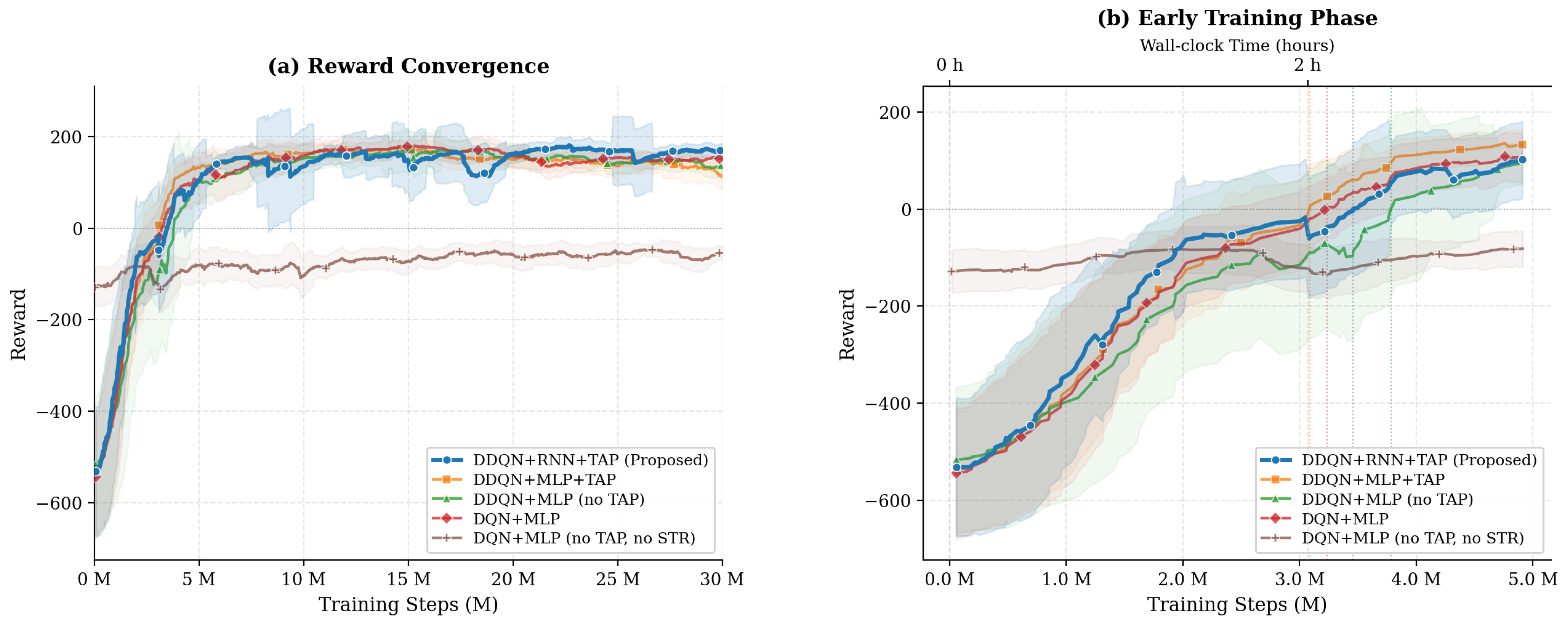
Training was conducted with Python 3.10 and PyTorch 1.10.2 on a workstation equipped with an Intel Core i9-11900 (8-core, 2.5 GHz), an NVIDIA RTX A5000 (24 GB VRAM), and 64 GB RAM. Figure 8 shows the episodic reward trajectories of the five learning-based variants (mean over three seeds, shaded $\pm 1\sigma$).

Early-phase convergence (Figure 8b). All Dueling DQN-based variants start near $-600$ and rise steeply within the first 2–3 M steps (∼0.8–1.2 h wall-clock). The proposed DDQN+RNN w/TAP crosses zero reward earliest (at ∼1.5 M steps) and reaches $+100$ by 3 M steps, despite showing the broadest confidence interval during this phase owing to the added variance of recurrent hidden-state initialization. DQN+MLP w/o TAP remains consistently negative, confirming that the Spatio-Temporal Reward (STR) is essential for escaping the initial reward floor.

Long-range stability (Figure 8a). Beyond 5 M steps, all TAP-augmented variants stabilize in the $+150$ to $+200$ band. The proposed DDQN+RNN w/TAP attains the highest asymptotic mean reward (≈$+190$) and the narrowest confidence interval after 10 M steps. DDQN+MLP w/o TAP plateaus 20–30 points below its TAP-equipped counterpart, quantifying the marginal effect of the TAP term on sustained reward accumulation. DQN+MLP with neither STR nor TAP fails to exceed zero reward over the entire 30 M-step horizon, rendering the sparse task effectively unlearnable within the given budget.

Three components contribute additively to training efficiency: STR escapes the negative-reward basin; TAP shaping accelerates convergence and raises the asymptotic ceiling; and the GRU encoder further improves both early convergence rate and steady-state stability.

5.3. Mission-Level Quantitative Performance

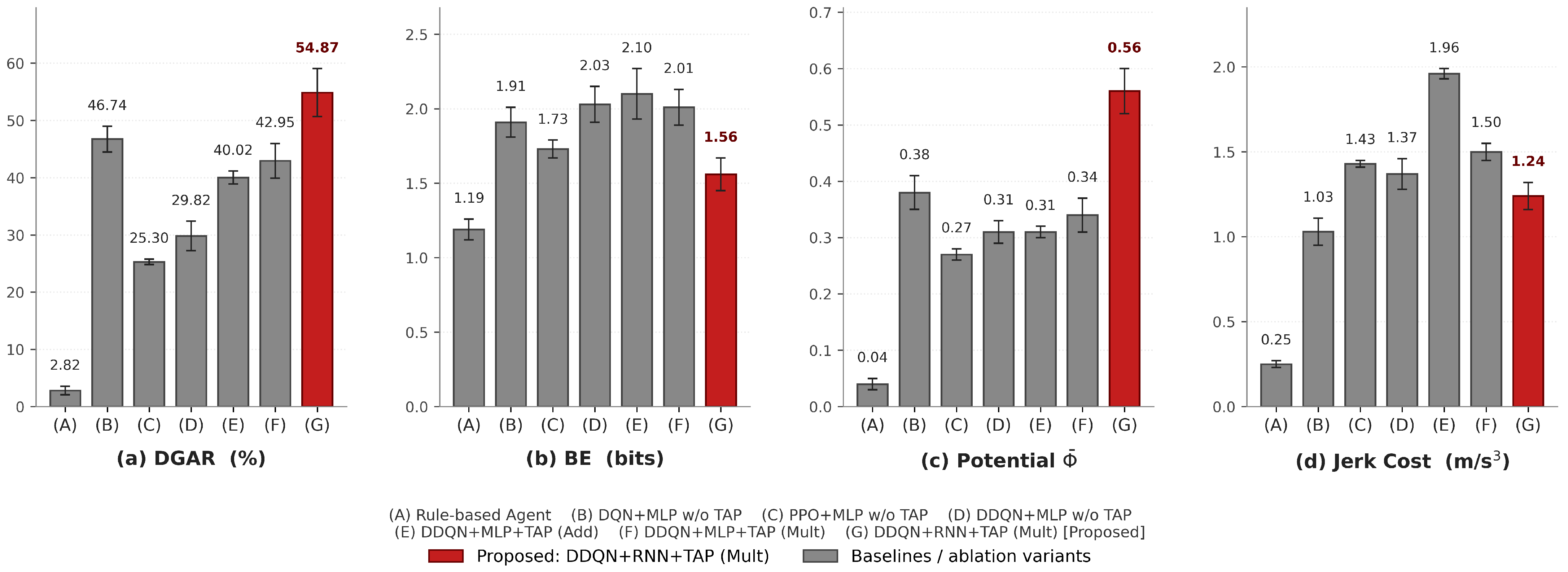
Mission-level performance is evaluated with four metrics: a task-success metric (DGAR), a tactical-geometric quality metric ($\overline{\mathrm{\Phi }}$), a behavioral-diversity metric (BE), and a physical metric ($J_{\mathrm{RMS}}$). All are reported as mean ± one standard deviation over $N_{\mathrm{ep}}$ evaluation episodes per training seed.

• Distance Goal Achievement Rate (DGAR). The fraction of steps within an evaluation episode during which the agent’s range to the ownship lies inside the engagement band, averaged across $N_{\mathrm{ep}}$ evaluation episodes:

  $$\mathrm{DGAR}={\displaystyle \frac{1}{N_{\mathrm{ep}}}}{\displaystyle \sum _{e=1}^{N_{\mathrm{ep}}}}{\displaystyle \frac{1}{T_e}}{\displaystyle \sum _{t=1}^{T_e}}\mathbf{1}\left[|d_{e,t}-d_{e,t}^{*}|\le \sigma \right],$$

  (32)

  where $T_e$ is the step count of episode e, $d_{e,t}$ is the agent–ownship range in episode e at step t, $d_{e,t}^{*}$ is the target distance, and $\mathbf{1}[·]$ is the indicator function.
• Behavioral Entropy (BE). The Shannon entropy of the empirical action distribution over the discrete action set $\mathcal{A}=\{a_1,\dots ,a_{\left|\mathcal{A}\right|}\}$:

  $$\mathrm{BE}=H\left(\pi \right)=-{\displaystyle \sum _{i=1}^{\left|\mathcal{A}\right|}}P\left(a_i\right){\log }_{2}P\left(a_i\right)\left[\mathrm{bits}\right],$$

  (33)

  with $P\left(a_i\right)=\left|\{t:a_t=a_i\}\right|/T$ the empirical action probability over an episode of length T. BE is bounded by $0\le \mathrm{BE}\le {\log }_2\left|\mathcal{A}\right|$: values close to the upper bound indicate near-uniform action use, while values close to 0 indicate a degenerate, near-deterministic policy.
• Mean Tactical Potential ($\overline{\mathbf{\Phi }}$). The time-averaged TAP score (Equation (24)) over an episode:

  $$\overline{\mathrm{\Phi }}={\displaystyle \frac{1}{T}}{\displaystyle \sum _{t=1}^T}\mathrm{\Phi }\left(s_t\right),\mathrm{\Phi }\left(s_t\right)\in (0,1.5].$$

  (34)
  Because $\mathrm{\Phi }={\varphi }_{\mathrm{pos}}·(1+0.5{\varphi }_{\mathrm{adv}})$ is multiplicatively coupled, $\overline{\mathrm{\Phi }}$ rewards sustained occupancy of the engagement band together with a favorable aspect; a brief instant of either condition alone does not raise $\overline{\mathrm{\Phi }}$ appreciably.
• Jerk Cost (${\mathit{J}}_{\mathbf{RMS}}$). The root-mean-square (RMS) of the per-step change in the agent’s longitudinal acceleration $a_t$ computed over the episode:

  $$\begin{array}{cc}\hfill \Delta a_t^{\mathrm{acc}}& \triangleq {\mathrm{clip}}_{\pm c}\left(a_{t+1}-a_t\right),t=1,\dots ,T-1,\hfill \\ \hfill J_{\mathrm{RMS}}& \triangleq \sqrt{{\displaystyle \frac{1}{T-1}}\sum _{t=1}^{T-1}{\left(\Delta a_t^{\mathrm{acc}}\right)}^2}\left[{\mathrm{m}/\mathrm{s}}^3\right],\hfill \end{array}$$

  (35)

  where $a_t^{\mathrm{acc}}$ is the scalar agent acceleration at step t. By penalizing abrupt acceleration changes, $J_{\mathrm{RMS}}$ serves as a smoothness surrogate: a high $\overline{\mathrm{\Phi }}$ combined with a low $J_{\mathrm{RMS}}$ shows that the tactical advantage is achieved with executable maneuvers rather than high-frequency control chatter infeasible on a real USV.

Figure 9 visualizes the mission-level ablation metrics summarized in

Table 7. Ablation study results (mean ± standard deviation).

Architecture	DGAR (%)	BE	Potential ($\overline{\mathbf{\Phi }}$)	Jerk
(A) Rule-based Agent	$2.82\pm 0.74$	$1.19\pm 0.07$	$0.04\pm 0.01$	$0.25\pm 0.02$
(B) DQN+MLP w/o TAP	$46.74\pm 2.25$	$1.91\pm 0.10$	$0.38\pm 0.03$	$1.03\pm 0.08$
(C) PPO+MLP w/o TAP	$25.30\pm 0.47$	$1.73\pm 0.06$	$0.27\pm 0.01$	$1.43\pm 0.02$
(D) DDQN+MLP w/o TAP	$29.82\pm 2.57$	$2.03\pm 0.12$	$0.31\pm 0.02$	$1.37\pm 0.09$
(E) DDQN+MLP w/ TAP (Add.)	$40.02\pm 1.13$	$2.10\pm 0.17$	$0.31\pm 0.01$	$1.96\pm 0.03$
(F) DDQN+MLP w/ TAP (Mult.)	$42.95\pm 3.03$	$2.01\pm 0.12$	$0.34\pm 0.03$	$1.50\pm 0.05$
(G) DDQN+RNN w/ TAP (Mult.) [Proposed]	$\mathbf{54.87}\pm \mathbf{4.19}$	$\mathbf{1.56}\pm \mathbf{0.11}$	$\mathbf{0.56}\pm \mathbf{0.04}$	$\mathbf{1.24}\pm \mathbf{0.08}$

. Table 7 shows the result of the ablation test. The DDQN+RNN w/TAP attains a DGAR of $54.87\%$, an improvement of $25.05$% (relative $+84.0\%$) over DDQN+MLP without TAP and of $52.05$% (relative $+18.5\times$) over the rule-based CGF. Relative to the strongest learning baseline (DQN+MLP without TAP, $46.74\%$), the proposed model improves DGAR by $8.13$ percentage points; we report this contrast explicitly to avoid benchmarking only against the weaker DDQN+MLP variant. The marginal effect of the TAP shaping term alone accounts for $+13.13$%, while the further incorporation of the GRU recurrent encoder contributes an additional $+11.92$%. The proposed model also attains the highest mean tactical potential ($\overline{\mathrm{\Phi }}=0.56$), and the lowest Jerk among the learning-based variants ($1.24$), indicating that the agent achieves mission objectives more frequently while sustaining tactically advantageous geometry with smoother trajectories.

Notably, DQN+MLP w/o TAP ($46.74\%$) outperforms both DDQN+MLP w/o TAP ($29.82\%$) and DDQN+MLP w/ TAP ($42.95\%$). This non-monotonicity reflects a known interaction between the dueling decomposition and low-dimensional encoders. In a compact 31-dimensional state with a six-action set, decoupling $V\left(s\right)$ and $A(s,a)$ without recurrent temporal context can amplify value-estimation variance, since the mean-subtraction term propagates noise across actions under sparse tactical feedback. Wang et al. [31] validated the dueling architecture in high-dimensional visual domains. The GRU encoder restores and exceeds the dueling benefit by stabilizing the advantage estimate through temporal aggregation. Finally, the lower BE of the proposed model ($1.56$, the lowest among the learning-based variants, versus $1.73$–$2.03$ for the no-TAP variants), together with the lowest Jerk Cost, confirms that TAP shaping yields a more concentrated and decisive tactical repertoire. We adopt the convention that lower behavioral entropy is desirable here, as it reflects committed rather than indecisive maneuvering, and we use this interpretation consistently throughout.

Statistical Significance of the Ablation Contrasts

Because the ablation rests on three independent seeds per architecture, we report inferential statistics for the key contrasts rather than relying on point estimates alone. For each pair we apply Welch’s two-sided t-test (unequal variances) on the per-seed DGAR, report Cohen’s d (pooled standard deviation) as the effect size and the $95\%$ confidence interval of the mean difference, and control the family-wise false-discovery rate across the five contrasts using the Benjamini–Hochberg procedure at $q=0.10$. The results are summarized in

Table 8. Statistical significance of the principal ablation contrasts (Welch’s t-test on DGAR, $n=3$ seeds per variant; $p_{\mathrm{BH}}$ is the Benjamini–Hochberg-adjusted p-value at $q=0.10$).

Contrast	ΔDGAR (pp)	Welch t	p	${\mathit{p}}_{\mathbf{BH}}$	Cohen’s d	95% CI
(G) Proposed vs. (D) DDQN+MLP w/o TAP	$+25.05$	$8.83$	$0.002$	$0.010$	$7.21$	$[16.5,33.6]$
(G) Proposed vs. (B) DQN+MLP (strongest baseline)	$+8.13$	$2.96$	$0.058$	$0.072$	$2.42$	$[-0.5,16.8]$
(F) Multiplicative vs. (E) Additive TAP	$+2.93$	$1.57$	$0.230$	$0.230$	$1.28$	$[-3.7,9.5]$
(G) Recurrent vs. (F) Feedforward	$+11.92$	$3.99$	$0.020$	$0.033$	$3.26$	$[3.3,20.5]$
(F) TAP-Mult. vs. (D) no-TAP	$+13.13$	$5.72$	$0.005$	$0.013$	$4.67$	$[6.7,19.6]$

.

Three observations follow. First, the contributions of the multiplicative TAP term over the no-TAP variant (F vs. D) and of the recurrent encoder (G vs. F) are statistically significant after correction ($p_{\mathrm{BH}}=0.013$ and $0.033$, with very large effect sizes $d=4.67$ and $3.26$). Second, and consistent with the three-seed limitation, the improvement of the proposed model over the strongest baseline (G vs. B) does not reach significance at the $0.05$ level after correction ($p_{\mathrm{BH}}=0.072$; the $95\%$ confidence interval $[-0.5,16.8]$ narrowly includes zero), even though the effect size is large ($d=2.42$); we therefore temper this particular ordering claim and note it as motivation for additional seeds. Third, the multiplicative-versus-additive contrast (F vs. E) shows a large effect size ($d=1.28$) but is not significant at $n=3$ ($p=0.230$), indicating that the coupling benefit, while consistent in direction, is under-powered at the current seed count. These results are discussed further in the limitations (Section 6).

5.4. Reward-Aligned Verification of the Multiplicative TAP Coupling

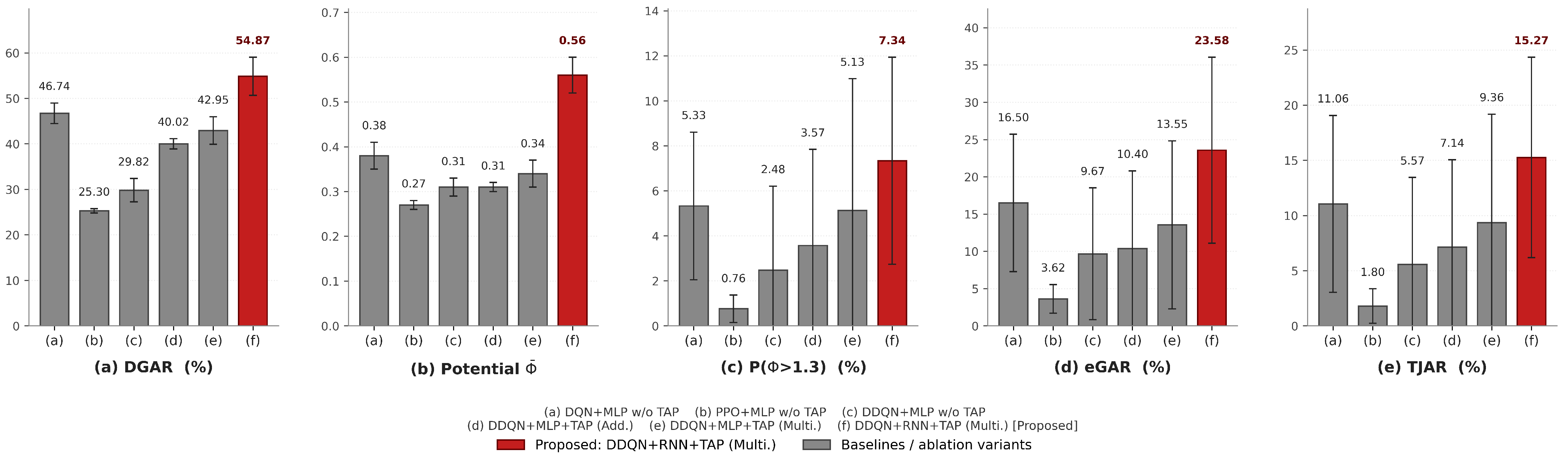
The mission-level metrics in Section 5.3 show that TAP-DDQN outperforms the baselines, but they do not isolate whether the gain is produced by the multiplicative TAP formulation. To test this point directly, we evaluate five reward-aligned diagnostics computed during inference over 500 evaluation episodes.

The diagnostics are DGAR, mean tactical potential $\overline{\mathrm{\Phi }}$, the high-score fraction $P(\mathrm{\Phi }>1.3)$, the effective goal achievement rate (eGAR), the Tactical Joint Achievement Rate (TJAR). TJAR and eGAR directly test whether distance and aspect conditions are satisfied jointly:

$$\mathrm{TJAR}=\mathbb{P}\left({\varphi }_{\mathrm{pos}}\left(s_t\right)>0.5\wedge {\varphi }_{\mathrm{adv}}\left(s_t\right)>0.7\right),$$

(36)

$$\mathrm{eGAR}=\mathbb{P}\left(|d\left(s_t\right)-d^{*}|<\sigma \wedge {\varphi }_{\mathrm{adv}}\left(s_t\right)>0.5\right).$$

(37)

Unlike the mission-success metrics of Section 5.3, these five statistics are computed on the scalar quantities that the TAP reward actively shapes during training, so improvements on them can be clearly attributed to the reward signal that TAP-DDQN optimizes. The gating thresholds are geometrically standard rather than tuned: ${\varphi }_{\mathrm{pos}}>0.5$ is the Gaussian half-maximum criterion, equivalent to $|d-d^{*}|<\sigma \sqrt{2\ln 2}\approx 589$ m (the full-width-at-half-maximum band of the engagement ring), while ${\varphi }_{\mathrm{adv}}>0.5$ and $>0.7$ correspond to the better-than-neutral and pursuit-dominant aspect sectors, respectively (head-on geometry gives ${\varphi }_{\mathrm{adv}}=0.5$ by construction). Because these thresholds are applied identically to every variant as post hoc diagnostics, they do not enter training and cannot bias the relative ordering. Threshold-gated fractions are, however, inherently higher-variance across seeds than continuous averages such as DGAR and $\overline{\mathrm{\Phi }}$, because episodes near a threshold flip categorically; this explains the broader error bars of P, eGAR, and TJAR.

Figure 10 visualizes the reward-aligned diagnostics summarized in

Table 9. Reward-aligned multi-dimensional verification of the multiplicative TAP coupling.

	(A) Marginal	(B) Aggregate of $\overline{\mathbf{\Phi }}$		(C) Joint Conditions
Model	DGAR (%)	Potential ($\overline{\mathbf{\Phi }}$)	P($\mathbf{\Phi }$ > 1.3) (%)	eGAR (%)	TJAR (%)
DQN+MLP w/o TAP	$46.74\pm 2.25$	$0.38\pm 0.03$	$5.33\pm 3.28$	$16.50\pm 9.23$	$11.06\pm 8.01$
PPO+MLP w/o TAP	$25.30\pm 0.47$	$0.27\pm 0.01$	$0.76\pm 0.61$	$3.62\pm 1.93$	$1.80\pm 1.56$
DDQN+MLP w/o TAP	$29.82\pm 2.57$	$0.31\pm 0.02$	$2.48\pm 3.73$	$9.67\pm 8.84$	$5.57\pm 7.88$
DDQN+MLP w/TAP (Add.)	$40.02\pm 1.13$	$0.31\pm 0.01$	$3.57\pm 4.27$	$10.40\pm 10.40$	$7.14\pm 7.92$
DDQN+MLP w/TAP (Multi.)	$42.95\pm 3.03$	$0.34\pm 0.03$	$5.13\pm 5.85$	$13.55\pm 11.28$	$9.36\pm 9.82$
DDQN+RNN w/ TAP (Multi.)	$\mathbf{54.87}\pm \mathbf{4.19}$	$\mathbf{0.56}\pm \mathbf{0.04}$	$\mathbf{7.34}\pm \mathbf{4.60}$	$\mathbf{23.58}\pm \mathbf{12.48}$	$\mathbf{15.27}\pm \mathbf{9.08}$

. Table 9 shows a consistent ordering across all five diagnostics. The proposed model attains the highest DGAR, $\overline{\mathrm{\Phi }}$, $P(\mathrm{\Phi }>1.3)$, eGAR, and TJAR, indicating that it not only enters the engagement band more often, but also maintains tactical aspect conditions once inside the band. The eGAR ratio is likewise highest for the proposed model, confirming that its ring-interior states are of higher tactical quality. Also, the experiments validate multiplicative TAP shaping as an effective and deployment-compatible approach for USV tactical autonomy and intelligent adversary generation in naval training environments.

5.5. Qualitative Analysis of Agent Behavior

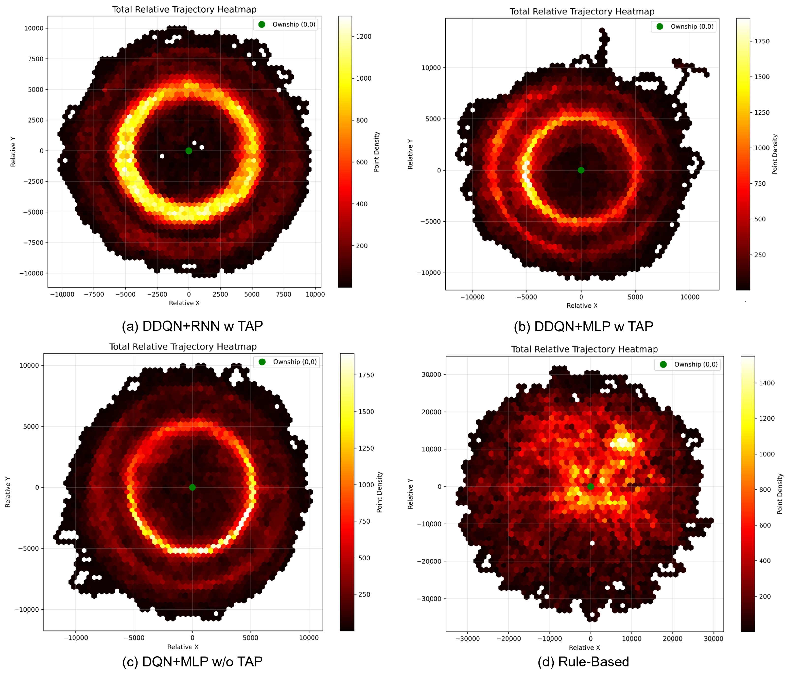
The physical manifestation is captured in the spatial heatmaps of Figure 11. The proposed model sustains a high-density arc within the ownship’s rear-quarter sector. The MLP variant with TAP (Figure 11b) recovers a ring-shaped concentration around $d^{*}$ but with larger angular dispersion, isolating the GRU’s role in providing the temporal context required for stable angular positioning. Taken together, these qualitative patterns are consistent with the quantitative metrics: the higher BE of no-TAP variants corresponds to their isotropic spatial distributions, whereas the proposed framework achieves simultaneous tactical precision and maneuver smoothness, validating the complementary roles of aspect-aware potential shaping and recurrent temporal memory.

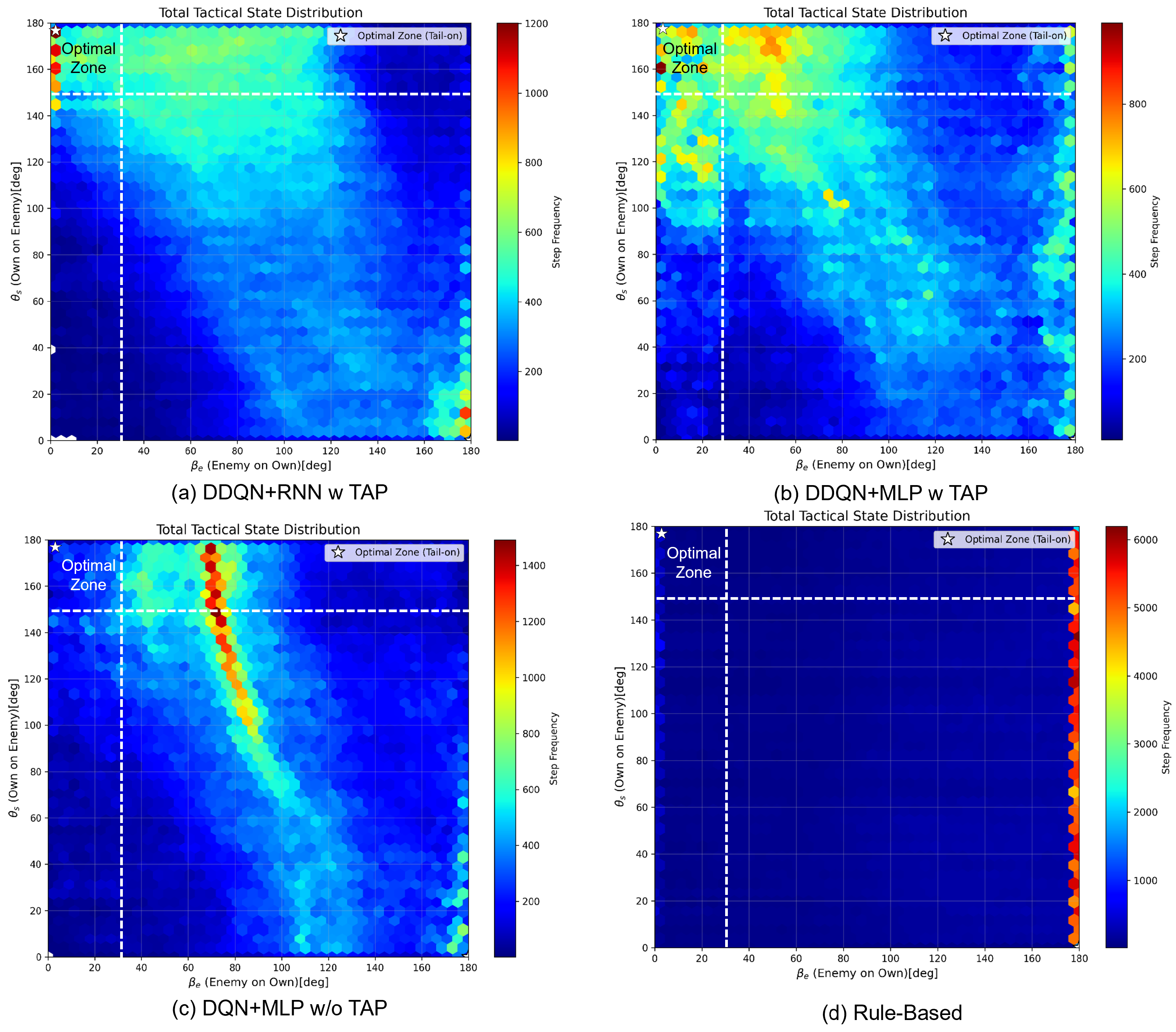
The state distribution analysis in Figure 12 shows that the proposed model concentrates states in the tactically optimal angular band (${\theta }_s\approx 0°$–$30°$), exactly the high-reward region defined by ${\varphi }_{\mathrm{adv}}$. Removing TAP (Figure 12c,d) restores a near-uniform angular spread, confirming that the tactical orientation is primarily driven by the proposed reward shaping.

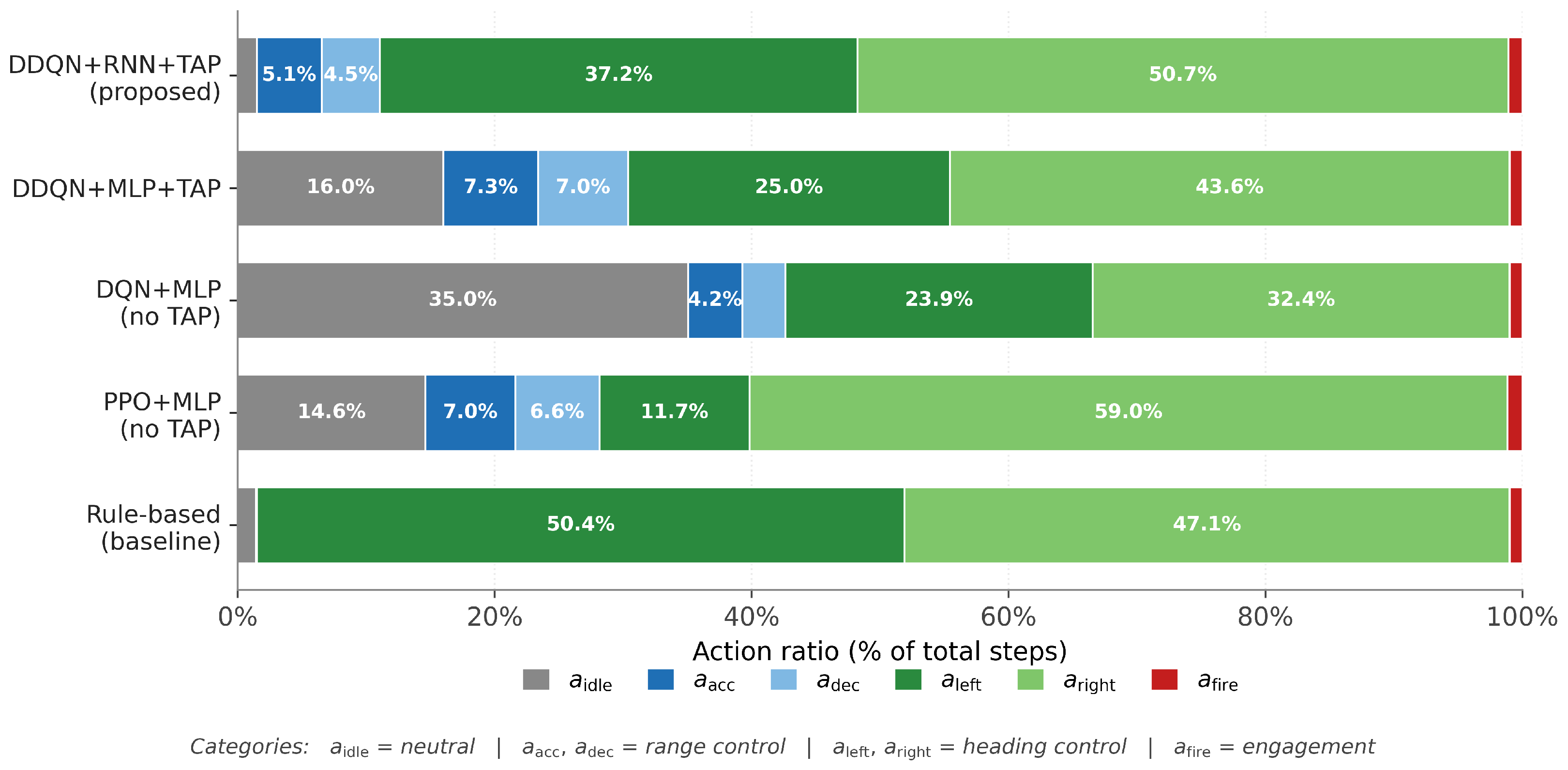
The action distribution in Figure 13 reveals the policy mechanism underlying the spatial and angular patterns of Figure 11 and Figure 12. First, the proposed agent assigns $87.84\%$ of its steps to turning actions, which directly explains the ring-bound, rear-quarter concentration of Figure 11a. It sustained tail-on alignment requiring continuous corrections of bearing, and the recurrent encoder enables these corrections without idle operation, $a_{\mathrm{idle}}$. Second, removing recurrent memory raises the idle ratio from $1.5\%$ to $16.0\%$, and removing TAP entirely further raises it to $14.6$–$35.0\%$. This rising idle ratio is the action-level signature of a partial policy collapse under sparse reward and parallels the rising Behavioral Entropy reported in Table 7. Because the no-TAP policies do not explore a richer behavioral repertoire, they default to no operation more often. Third, the rule-based baseline allocates $97.5\%$ of its steps to turning actions and never modulates speed, confirming that the scripted CGF cannot trade off range and aspect simultaneously.

6. Discussion

This section analyzes the quantitative and qualitative results of the proposed intelligent maneuvering framework through a series of ablation studies and comparative analyses. We focus on the mechanism of the multiplicative TAP coupling, the temporal reasoning capabilities provided by the GRU module, and the practical implications for legacy naval training systems.

6.1. Mechanism of the Multiplicative TAP Coupling

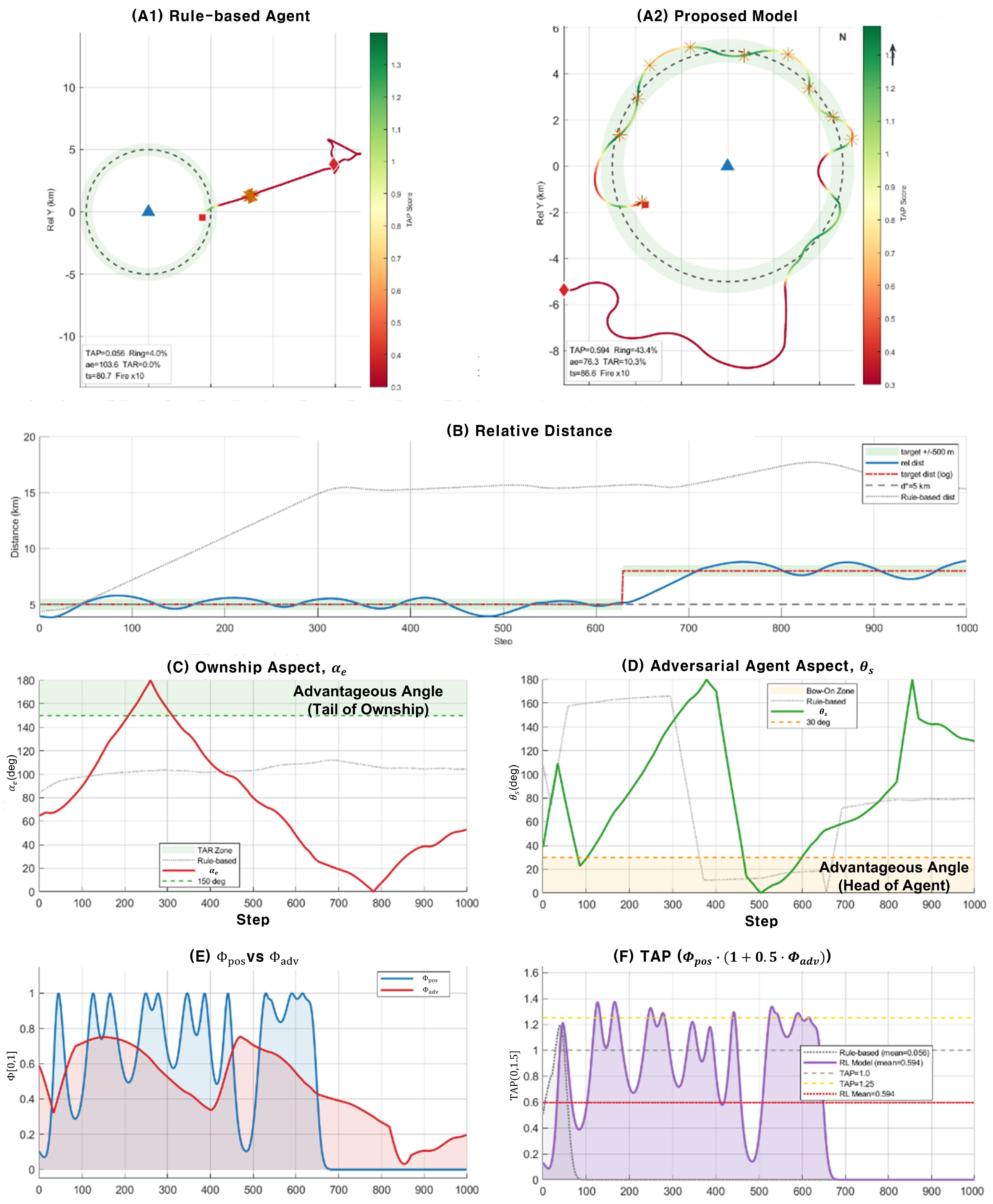
We chose the multiplicative form $\mathrm{\Phi }\left(s\right)={\varphi }_{\mathrm{pos}}\left(s\right)·\left(1+0.5{\varphi }_{\mathrm{adv}}\left(s\right)\right)$ instead of the additive form used in [47,48]. Figure 14 shows what this choice does in practice. Figure 14E shows ${\varphi }_{\mathrm{pos}}$ oscillating up and down as the agent passes through the ring; ${\varphi }_{\mathrm{adv}}$ stabilizes around 0.7–0.9 only after the agent approaches the ring. Outside the ring the angular gradient is essentially shut off by the multiplicative gate. Figure 14F shows that the instantaneous $\mathrm{\Phi }\left(s\right)$ of the proposed policy peaks in the 1.2–1.4 band, whereas the rule-based agent remains near 0.05–0.08. The agent is rewarded only when it achieves both ring proximity and heading alignment simultaneously, not for either alone.

This behavior is consistent with the policy-invariance argument in Section 3.4.4: the shaping signal becomes dense where tactical guidance is useful, but it does not encourage irrelevant long-range aspect optimization. The heatmaps in Figure 11 and the reward-aligned diagnostics in Table 9 support the interpretation. The proposed policy exhibits the clearest rear-quarter concentration and the highest joint distance–aspect statistics, whereas additive or no-TAP variants do not reproduce this pattern. Consistently, Figure 13 shows that all TAP-trained variants ($a_{\mathrm{idle}}=1.5$–$16.0\%$) maintain substantially lower idle ratios than the no-TAP variants ($14.6$–$35.0\%$), demonstrating that the dense, range-gated gradient produced by the multiplicative coupling prevents the policy collapse onto inaction that sparse-reward training otherwise induces.

6.2. Role of Recurrent Temporal Memory

The ablation pattern in Section 5.3, where DQN+MLP without TAP unexpectedly outperforms DDQN+MLP variants, clarifies the specific contribution of the GRU encoder. In this compact state space, feedforward Dueling can increase value-estimation variance instead of reducing it, because the advantage decomposition is not supported by sufficient temporal context. Recurrent aggregation mitigates this issue by smoothing the advantage estimate across long engagements. Empirically, adding GRU to DDQN+MLP with multiplicative TAP improves DGAR, yields the lowest Jerk Cost among the learning-based variants, and produces the narrowest long-range reward variance in Figure 8. This GRU contribution is also directly visible at the action level: Figure 13 shows that the recurrent DDQN+RNN+TAP policy spends $87.84\%$ of its steps actively turning, whereas the otherwise identical DDQN+MLP+TAP feedforward variant falls into the idle action $16\%$ of the time, an order-of-magnitude shift that mirrors the recurrent/non-recurrent gap on $\overline{\mathrm{\Phi }}$.

6.3. Implications for USV Tactical Autonomy and Naval Training System

Beyond its quantitative performance advantages in simulated tactical scenarios, the proposed TAP-DDQN framework introduces a dual-use paradigm that bridges maritime requirements with autonomy and regulatory compliance. In contemporary ocean engineering, USV platforms are increasingly expected to operate in multi-mission roles such as harbor patrolling and asset escort under standard peace-time conditions. The learned guidance policy of the TAP-DDQN agent demonstrates how these conflicting operational objectives can be reconciled within a single, policy-invariant control architecture.

Under standard patrolling or cooperative escort phases, the agent’s converged behavior—which stabilizes into a non-crossing, stern-quarter shadowing orbit at a relative bearing of ${\theta }_s\in [0°,30°]$ abaft the target’s beam—conceptually and geometrically satisfies the safety requirements of COLREGs Rule 13 (Overtaking Rule) [53]. Conversely, when a non-cooperative intruder exhibits erratic maneuvers or deploys high-speed dynamic hazards, the priority of the USV shifts immediately to platform survivability. This rapid transition from compliant, stable tracking to highly agile, non-linear evasive maneuvers functionally operationalizes the core mandate of COLREGs Rule 2 (General Prudential Rule) [53]. The proposed multiplicative potential formulation mathematically allows the USV to temporarily prioritize active dodging of dynamic hazards over strict path-following, indicating that the policy balances standard traffic rules and emergency survival protocols while mitigating the chattering and local-minima vulnerabilities associated with potential-based methods such as APF-RADQN [54]. Consequently, the policy model developed in this research serves a dual use. It can be deployed on operational USV platforms to enhance maritime autonomy, or used to generate highly realistic, non-scripted adversarial CGFs for shipboard OBTSs that train human operators against realistic threat maneuvers.

6.4. Limitations

Four limitations of the present study merit explicit discussion. First, statistical robustness is based on three independent seeds per configuration; although this is consistent with common practice in naval DRL studies given the 30 M-step training cost per seed, broader seed coverage would tighten the confidence intervals. The multi-dimensional verification of Table 9 mitigates this concern for the reward-aligned diagnostics specifically: the dispersions reported in that table for the proposed model ($\pm 0.04$ for $\overline{\mathrm{\Phi }}$, $\pm 9.08$ pp for TJAR, and $\pm 12.48$ pp for eGAR) are comparable to, and for the joint-condition metrics, larger than, the cross-variant gaps, so these diagnostics are interpreted together with the significance tests of Table 8. But this lower-variance regime does not extend to mission-success metrics such as DGAR. Second, because the evaluation is restricted to 1-vs-1 surface engagements, multi-agent swarm interactions and underwater or airborne adversaries remain outside the current scope. Similarly, obstacle-laden or littoral environments with COLREGs-constrained traffic would require augmenting the constraint reward with collision-avoidance terms and extending the aspect geometry accordingly; the potential-based structure of TAP itself carries over unchanged. Third, the reward decomposition was designed around a specific tactical doctrine. Alternative doctrines such as beam-aspect engagement or anti-submarine screening would require re-specification of ${\varphi }_{\mathrm{pos}}$ and ${\varphi }_{\mathrm{adv}}$. Fourth, the reward-aligned diagnostics of Table 9 were computed at specific engagement-band parameters. A formal $\sigma$-sweep curriculum remains for future work. We hypothesize, but do not verify, that the qualitative ordering across the evaluated learning-based variants would be preserved under moderate changes of $\sigma$; the continuity of the potential in $\sigma$ (Equation (25)) does not by itself establish this. A systematic analysis of the angular weight $w_{\mathrm{ang}}$ is likewise not provided and is left to future work. The absolute magnitudes of TJAR and eGAR are expected to scale with the chosen band width.

7. Conclusions

This paper presented TAP-DDQN, a deep reinforcement learning framework for on-board engagement-level tactical decision-making in USVs, which is simultaneously deployable as a dual-use intelligent adversarial agent inside shipboard OBTS. The framework targets the discrete action interfaces, bounded inference latency, and non-invasive software constraints that distinguish operational maritime systems from generic RL research simulators, and it explicitly addresses the gap between low-level marine continuous control and engagement-level tactical autonomy identified in prior work.

The principal methodological contribution is the multiplicative Tactical Approach Potential (TAP) reward shaping that couples a distance-ring potential with an aspect-aware tactical term. The multiplicative coupling ensures that angular guidance becomes active only inside the tactical engagement band and is strongly attenuated at long range, suppressing the inductive bias that additive formulations inject by construction. TAP is paired with an explainable component reward decomposition, a GRU-augmented Dueling DQN, and a Dynamic Target Curriculum, and is integrated with a legacy maritime combat-management simulator through the non-invasive TRNLE wrapper, which requires no modification of the underlying software.

Across 30 million training steps and three independent seeds in a 1-vs-1 surface-engagement scenario, the proposed TAP-DDQN attains a DGAR of $54.87\pm 4.19\%$, exceeding the rule-based CGF baseline by more than an order of magnitude and the DDQN+MLP variant without TAP by $25.05\%$ (and the strongest learning baseline, DQN+MLP without TAP, by $8.13$ percentage points). Ablation isolates the marginal contributions: multiplicative TAP shaping alone contributes $+13.13\%$ in DGAR over the no-TAP baseline, and the GRU recurrent encoder contributes an additional $+11.92\%$ under identical shaping. The Jerk Cost of $1.24$ further confirms that recurrent temporal memory produces smoother trajectories suitable for naval training and on-board deployment.

Beyond aggregated mission metrics, a set of reward-aligned diagnostics computed on the scalar quantities that the multiplicative TAP establishes that the performance gains originate from the multiplicative coupling itself rather than from incidental architectural factors. The proposed agent simultaneously attains the highest values across all reward-aligned dimensions, exceeding the strongest learning baseline by 17–$47\%$ on every dimension. Qualitative analyses further show that the learned policy approaches the desired engagement ring, stabilizes a favorable stern-quarter geometry, and exhibits more coherent maneuver behavior than rule-based or additive-reward baselines.

At the systems-integration level, the TRNLE wrapper bridges DRL training and a legacy combat management system without any hardware or software modification. A single trained policy can therefore be deployed in two applications as an on-board tactical decision-making module for autonomous USVs, and as an adversarial agent for human-in-the-loop OBTS. On the deployment side, the trained policy is a compact single-GRU network (Table 6) whose 30 M-step training is a one-time offline cost. In addition, standard model-compression techniques such as post-training quantization, pruning, and distillation provide a direct path to embedded mission hardware. We further plan a staged live–virtual–constructive (LVC) validation in which the trained policy is coupled to the operational CMS through the same non-invasive TRNLE wrapper for hardware-in-the-loop trials.

Future work will extend this dual-use high-level decision-making framework to multi-agent cooperative-adversarial scenarios and heterogeneous USV-UAV swarm coordination. We also plan to explore hierarchical tactical reasoning under partial observability and real-time integration with C2/C4I systems under extreme environmental and communication uncertainties.

References

1. Wang, H.; Zhou, Z.; Jiang, J.; Deng, W.; Chen, X. Autonomous Air Combat Maneuver Decision-Making Based on PPO-BWDA. IEEE Access 2024, 12, 119116–119132. [Google Scholar] [CrossRef] [Scilit]
2. Wang, N.; Li, Z.; Liang, X.; Hou, Y.; Yang, A. A review of deep reinforcement learning methods and military application research. Math. Probl. Eng. 2023, 2023, 7678382. [Google Scholar] [CrossRef] [Scilit]
3. Brockman, G. OpenAI Gym. arXiv 2016, arXiv:1606.01540. [Google Scholar]
4. Kurach, K.; Raichuk, A.; Stańczyk, P.; Zając, M.; Bachem, O.; Espeholt, L.; Riquelme, C.; Vincent, D.; Michalski, M.; Bousquet, O.; et al. Google Research Football: A Novel Reinforcement Learning Environment. arXiv 2020, arXiv:1907.11180. [Google Scholar]
5. Samvelyan, M.; Rashid, T.; De Witt, C.S.; Farquhar, G.; Nardelli, N.; Rudner, T.G.; Hung, C.M.; Torr, P.H.; Foerster, J.; Whiteson, S. The starcraft multi-agent challenge. arXiv 2019, arXiv:1902.04043. [Google Scholar]
6. Bingham, B.; Agüero, C.; McCarrin, M.; Klamo, J.; Malia, J.; Allen, K.; Lum, T.; Rawson, M.; Waqar, R. Toward Maritime Robotic Simulation in Gazebo. In Proceedings of the MTS/IEEE OCEANS Conference, Seattle, WA, USA, 27–31 October 2019. [Google Scholar] [CrossRef] [Scilit]
7. Paravisi, M.; Santos, D.H.; Jorge, V.; Heck, G.; Gonçalves, L.M.; Amory, A. Unmanned Surface Vehicle Simulator with Realistic Environmental Disturbances. Sensors 2019, 19, 1068. [Google Scholar] [CrossRef] [Scilit] [PubMed]
8. Bae, J.H.; Jung, H.; Kim, S.; Kim, S.; Kim, Y.D. Deep reinforcement learning-based air-to-air combat maneuver generation in a realistic environment. IEEE Access 2023, 11, 26427–26440. [Google Scholar] [CrossRef] [Scilit]
9. Hu, D.; Yang, R.; Zuo, J.; Zhang, Z.; Wu, J.; Wang, Y. Application of deep reinforcement learning in maneuver planning of beyond-visual-range air combat. IEEE Access 2021, 9, 32282–32297. [Google Scholar] [CrossRef] [Scilit]
10. Piao, H.Y.; Yang, S.; Chen, H.; Li, J.; Yu, J.; Peng, X.; Yang, X.; Yang, Z.; Sun, Z.; Chang, Y. Discovering Expert-Level Air Combat Knowledge via Deep Excitatory-Inhibitory Factorized Reinforcement Learning. ACM Trans. Intell. Syst. Technol. 2024, 15, 1–28. [Google Scholar] [CrossRef] [Scilit]
11. Roessingh, J.J.; Toubman, A.; van Oijen, J.; Poppinga, G.; Hou, M.; Luotsinen, L. Machine learning techniques for autonomous agents in military simulations—Multum in Parvo. In Proceedings of the 2017 IEEE International Conference on Systems, Man, and Cybernetics (SMC); IEEE: Piscataway, NJ, USA, 2017; pp. 3445–3450. [Google Scholar] [CrossRef] [Scilit]
12. Boron, J.; Darken, C. Developing combat behavior through reinforcement learning in wargames and simulations. In Proceedings of the 2020 IEEE Conference on Games (CoG); IEEE: Piscataway, NJ, USA, 2020; pp. 728–731. [Google Scholar] [CrossRef] [Scilit]
13. Dimitriu, A.; Michaletzky, T.V.; Remeli, V.; Tihanyi, V.R. A Reinforcement Learning Approach to Military Simulations in Command: Modern Operations. IEEE Access 2024, 12, 77501–77513. [Google Scholar] [CrossRef] [Scilit]
14. Narvekar, S.; Peng, B.; Leonetti, M.; Sinapov, J.; Taylor, M.E.; Stone, P. Curriculum learning for reinforcement learning domains: A framework and survey. J. Mach. Learn. Res. 2020, 21, 1–50. [Google Scholar] [CrossRef] [Scilit]
15. Hutsebaut-Buysse, M.; Mets, K.; Latré, S. Hierarchical reinforcement learning: A survey and open research challenges. Mach. Learn. Knowl. Extr. 2022, 4, 172–221. [Google Scholar] [CrossRef] [Scilit]
16. Ma, H.; Vo, T.V.; Leong, T.Y. Mixed-Initiative Bayesian Sub-Goal Optimization in Hierarchical RL. In Proceedings of the 23rd International Conference on Autonomous Agents and MultiAgent Systems (AAMAS); IFAAMAS: Richland, SC, USA, 2024; pp. 1328–1336. [Google Scholar]
17. Ng, A.Y.; Harada, D.; Russell, S. Policy invariance under reward transformations: Theory and application to reward shaping. Proc. ICML 1999, 99, 278–287. [Google Scholar]
18. Cooley, T.; Oswalt, I.; Oxford, M.; Park, L. Operationalizing Artificial Intelligence in Simulation Based Training. In Proceedings of the 2021 Interservice/Industry Training, Simulation, and Education Conference (I/ITSEC), Orlando, FL, USA, 29 November–3 December 2021. [Google Scholar]
19. Black, S.; Darken, C. Scaling Intelligent Agents in Combat Simulations for Wargaming. arXiv 2024, arXiv:2402.06694. [Google Scholar]
20. Qiao, Y.; Yin, J.; Wang, W.; Duarte, F.; Yang, J.; Ratti, C. Survey of Deep Learning for Autonomous Surface Vehicles in Marine Environments. IEEE Trans. Intell. Transp. Syst. 2023, 24, 3678–3701. [Google Scholar] [CrossRef] [Scilit]
21. Hong, L.; Liu, L.; Peng, Z.; Zhang, F. Control of Marine Robots in the Era of Data-Driven Intelligence. Annu. Rev. Control. Robot. Auton. Syst. 2025, 9, 243–272. [Google Scholar] [CrossRef] [Scilit]
22. International Maritime Organization. Interim Guidelines for MASS Trials; Msc.1/circ.1604; Adopted at MSC 101; International Maritime Organization (IMO): London, UK, 2019. [Google Scholar]
23. Wu, C.; Yu, W.; Li, G.; Liao, W. Deep reinforcement learning with dynamic window approach based collision avoidance path planning for maritime autonomous surfaces. Ocean Eng. 2023, 284, 115208. [Google Scholar] [CrossRef] [Scilit]
24. Wang, C.; Zhang, X.; Yang, Z.; Bashir, M.; Lee, K. Collision Avoidance for Autonomous Ship Using Deep Reinforcement Learning and Prior-Knowledge-Based Approximate Representation. Front. Mar. Sci. 2023, 9, 1084763. [Google Scholar] [CrossRef] [Scilit]
25. Tam, C.; Bucknall, R.; Greig, A. Review of Collision Avoidance and Path Planning Methods for Ships in Close Range Encounters. J. Navig. 2009, 62, 455–476. [Google Scholar] [CrossRef] [Scilit]
26. Jung, Y.R. A study on multi sensor track fusion algorithm for naval combat system. J. Korea Inst. Mil. Sci. Technol. 2007, 10, 34–42. [Google Scholar]
27. Go, Y. A Study on Bottom-Up Update of TPR-Tree for Target Indexing in Naval Combat Systems. J. Korea Inst. Mil. Sci. Technol. 2019, 22, 266–277. [Google Scholar]
28. Navy, U. Navy’s Newest Combat Simulator Trains Its First Ships; Technical Report; United States Navy: Washington, DC, USA, 2020. [Google Scholar]
29. Sutton, R.S.; Barto, A.G. Reinforcement Learning: An Introduction, 2nd ed.; MIT Press: Cambridge, MA, USA, 2018. [Google Scholar]
30. Mnih, V.; Kavukcuoglu, K.; Silver, D.; Rusu, A.A.; Veness, J.; Bellemare, M.; Graves, A.; Riedmiller, M.; Fidjeland, A.; Ostrovski, G.; et al. Human-level control through deep reinforcement learning. Nature 2015, 518, 529–533. [Google Scholar] [CrossRef] [Scilit] [PubMed]
31. Wang, Z.; Schaul, T.; Hessel, M.; van Hasselt, H.; Lanctot, M.; de Freitas, N. Dueling Network Architectures for Deep Reinforcement Learning. In Proceedings of the 33rd International Conference on Machine Learning (ICML), New York, NY, USA, 19–24 June 2016; pp. 1995–2003. [Google Scholar]
32. Cho, K.; van Merriënboer, B.; Gulcehre, C.; Bahdanau, D.; Bougares, F.; Schwenk, H.; Bengio, Y. Learning Phrase Representations using RNN Encoder–Decoder for Statistical Machine Translation. arXiv 2014, arXiv:1406.1078. [Google Scholar]
33. Coble, J.; Barton, A.; Darken, C.; Black, S. Optimizing Naval Movement Using Deep Reinforcement Learning. In Proceedings of the 2023 International Conference on Machine Learning and Applications (ICMLA); IEEE: Piscataway, NJ, USA, 2023; pp. 400–407. [Google Scholar]
34. Markowitz, J.; Sheffield, R.; Mullins, G. Maritime Platform Defense with Deep Reinforcement Learning. In Proceedings of the Artificial Intelligence and Machine Learning for Multi-Domain Operations Applications IV; SPIE: Bellingham, WA, USA, 2022; Volume 12113, pp. 423–429. [Google Scholar] [CrossRef] [Scilit]
35. Zhang, H.; Zhou, H.; Wei, Y.; Huang, C. Autonomous maneuver decision-making method based on reinforcement learning and Monte Carlo tree search. Front. Neurorobot. 2022, 16, 996412. [Google Scholar] [CrossRef] [Scilit]
36. Mei, J.; Li, G.; Huang, H. Deep Reinforcement-Learning-Based Air-Combat-Maneuver Generation Framework. Mathematics 2024, 12, 3020. [Google Scholar] [CrossRef] [Scilit]
37. Bae, J.H.; Kang, Y.; Yoon, S.; Kim, Y.; Kim, S. Aircraft Reinforcement Learning using Curriculum Learning. J. Korean Inst. Inf. Sci. Eng. (KIISE) 2021, 48, 707–712. [Google Scholar] [CrossRef] [Scilit]
38. Zhu, J.; Kuang, M.; Zhou, W.; Shi, H.; Zhu, J.; Han, X. Mastering air combat game with deep reinforcement learning. Def. Technol. 2024, 34, 295–312. [Google Scholar] [CrossRef] [Scilit]
39. Gorton, P.R.; Strand, A.; Brathen, K. A survey of air combat behavior modeling using machine learning. arXiv 2024, arXiv:2404.13954. [Google Scholar]
40. Bartsiokas, I.A.; Ntakolia, C.; Avdikos, G.; Lyridis, D.V. Intelligent Multi-Objective Path Planning for Unmanned Surface Vehicles via Deep and Fuzzy Reinforcement Learning. J. Mar. Sci. Eng. 2025, 13, 2285. [Google Scholar] [CrossRef] [Scilit]
41. Ntakolia, C.; Lyridis, D.V. A Swarm Intelligence Graph-Based Pathfinding Algorithm Based on Fuzzy Logic (SIGPAF): A Case Study on Unmanned Surface Vehicle Multi-Objective Path Planning. J. Mar. Sci. Eng. 2021, 9, 1243. [Google Scholar] [CrossRef] [Scilit]
42. Ntakolia, C.; Lyridis, D.V. A Comparative Study on Ant Colony Optimization Algorithm Approaches for Solving Multi-Objective Path Planning Problems in Case of Unmanned Surface Vehicles. Ocean Eng. 2022, 255, 111418. [Google Scholar] [CrossRef] [Scilit]
43. Wiewiora, E.; Cottrell, G.; Elkan, C. Principled methods for advising reinforcement learning agents. In Proceedings of the 20th International Conference on Machine Learning (ICML-03), Washington, DC, USA, 12–24 August 2003. [Google Scholar]
44. Gao, Y.; Toni, F. Potential-based reward shaping for hierarchical reinforcement learning. In Proceedings of the IJCAI, Buenos Aires, Argentina, 25–31 July 2015. [Google Scholar]
45. Asmuth, J.; Littman, M.L.; Zinkov, R. Potential-based shaping in model-based reinforcement learning. In Proceedings of the AAAI, Chicago, IL, USA, 13–17 July 2008. [Google Scholar]
46. Devlin, S.; Kudenko, D. Dynamic Potential-Based Reward Shaping. In Proceedings of the 11th International Conference on Autonomous Agents and Multiagent Systems (AAMAS), Valencia, Spain, 4–8 June 2012; pp. 433–440. [Google Scholar]
47. Zhang, P.; Wang, X.; Wang, Y.; Ma, Z.; Lu, J. Combat game strategy for unmanned surface vessels based on situational field PPO (SF-PPO). Ocean Eng. 2025, 316, 119853. [Google Scholar] [CrossRef] [Scilit]
48. Yang, K.; Dong, W.; Cai, M.; Jia, S.; Liu, R. UCAV Air Combat Maneuver Decisions Based on a Proximal Policy Optimization Algorithm with Situation Reward Shaping. Electronics 2022, 11, 2602. [Google Scholar] [CrossRef] [Scilit]
49. Li, Y.; Yuan, Y.; Cheng, Y.; Hua, L. Predictive Air Combat Decision Model with Segmented Reward Allocation. Complex Intell. Syst. 2024, 10, 7513–7530. [Google Scholar] [CrossRef] [Scilit]
50. Kun, Y.; Ao, S.; Nengwei, X.; Fang, D.; Maobin, L.; Chen, C. A review of reinforcement learning approaches for pursuit-evasion games. Chin. J. Aeronaut. 2025, 39, 103940. [Google Scholar] [CrossRef] [Scilit]
51. Wang, N.; Hou, Y.; Qiu, C.; You, Z. Underactuated Navigation Actor-Critic Deep Reinforcement Learning Framework for Holistic Path Planning of Uncrewed Surface Vehicles. IEEE Trans. Intell. Transp. Syst. 2025, 26, 21245–21256. [Google Scholar] [CrossRef] [Scilit]
52. Shin, H.; Ahn, J.; Ahn, J.H.; Kim, M.; Kim, J.; Kim, S. Constructing a Reinforcement Learning Environment Based on a Legacy Simulator for Training a Prototype Intelligent Simulation Agent for Surface Vessels. J. Korean Inst. Intell. Syst. 2025, 35, 163–170. [Google Scholar] [CrossRef] [Scilit]
53. International Maritime Organization. Convention on the International Regulations for Preventing Collisions at Sea, 1972 (COLREGs); International Maritime Organization: London, UK, 2003. [Google Scholar]
54. Mou, J.; Shi, B.; Wang, B.; Yu, C.; Wang, Y.; Zhong, F.; Zheng, L.; Wang, J.; Li, J. A novel reinforcement learning framework-based path planning algorithm for unmanned surface vehicle. Front. Mar. Sci. 2025, 12, 1641093. [Google Scholar] [CrossRef] [Scilit]
Figure 1. Overview of the TAP-DDQN framework. Model-training framework to train on-board policy for dual-use of the USV high-level decision module and adversary-agent generation for shipboard on-board training.
Jmse 14 01569 g001
Figure 2. Naval tactical geometry used in the engagement scenario. (a) Definition of the relative bearing, line-of-sight (LOS), and aspect-angle geometry between the adversarial agent and the ownship. (b) Schematic of the hazard and advantage zones used to interpret tactically favorable and unfavorable relative postures. (c) Concept diagram of tactical decision-making, considering the agent relative bearing θ s , the ownship aspect angle α e , the LOS, and the concentric radar detection and weapon engagement rings. These geometric elements jointly determine the region in which the aspect-aware potential ϕ adv becomes active. (d) Pursuit ( ϕ adv = 1 , most favorable), (e) Head-on ( ϕ adv = 1 / 2 , neutral), and (f) Tail-on ( ϕ adv = 0 , most unfavorable): tactical configurations at the extreme values of ϕ adv , merged from the previously separate figure.
Jmse 14 01569 g002
Figure 3. Schematic of the four-component reward decomposition. Each state transition s t s t + 1 produces four semantically distinct signals—the spatio-temporal reward r t STR (smooth distance approach), the constraint reward r t CON (speed and boundary safety), the weapon-firing reward r t WR (timely weapon use), and the tactical-potential shaping term F ( s t , s t + 1 ) derived from the multiplicative TAP Φ = ϕ pos · ( 1 + 0.5 ϕ adv ) (the principal contribution, red star)—which are summed into the total reward r t . The components are magnitude-isolated so that each can be interpreted and ablated independently.
Jmse 14 01569 g003
Figure 4. Distance potential ϕ pos . (a) One-dimensional Gaussian ring profile ϕ d = exp ( d d * ) 2 / ( 2 σ 2 ) for two engagement-band widths σ { 200 , 500 } m . (b) Two-dimensional spatial field centered at the designated engagement distance d * = 5 km with σ = 500 m . Overlaid reference circles mark the Optimal Standoff at d * (solid), the Weapon Range at 5 km (dashed), the Radar Detection Range at 8 km (dotted), and the Full Width at Half Maximum (FWHM) ring for σ = 500 m (dash-dot); the white triangle denotes the ownship.
Jmse 14 01569 g004
Figure 5. Geometric gating effect of the multiplicative Tactical Approach Potential (TAP) compared with additive aspect shaping. (a) Additive TAP: Additive shaping, ϕ pos + 0.5 ϕ adv maintains a non-zero angular gradient everywhere, inducing a heading bias before range alignment is achieved. (b) Multiplicative TAP: Proposed Multiplicative shaping, Φ = ϕ pos · ( 1 + 0.5 ϕ adv )  geometrically gates the angular signal by the distance-ring envelope, activating aspect shaping only inside the engagement band. (c) Radial cross-section: TAP’s pursuit and tail-on curves overlap outside the ring (no bias), whereas the additive formulation keeps a visible angular gap throughout. This gating preserves the policy-invariance condition without sacrificing dense tactical guidance inside the engagement band.
Jmse 14 01569 g005
Figure 6. Architecture of the TRNLE-based training and inference framework integrated with the Dueling DQN agent. The figure summarizes the major modules and the data flow between the simulator, the reinforcement learning model, and the control interface. Reward-shaping components are detailed in Figure 4 and Figure 5, and the full operator interface is shown in Figure 7.
Jmse 14 01569 g006
Figure 7. TRNLE User Interface, comprising the Training Display Region (left), the Basic Display Region (right, entity and engagement information), and the Control Panel Region (top). The interface capture is enlarged for annotation legibility.
Jmse 14 01569 g007
Figure 8. Reward convergence of the compared training configurations. (a) Full convergence trajectories over 30 million environment steps. (b) Magnified view of the early training phase, highlighting initial learning speed and wall-clock efficiency.
Jmse 14 01569 g008
Figure 9. Visual comparison of mission-level quantitative performance. Each panel reports one of the four metrics across the seven architectures (A–G); error bars indicate ± 1 standard deviation across three independent seeds. The proposed DDQN+RNN+TAP (Mult.) architecture (G, red) attains the highest DGAR (54.87%) and the highest mean tactical potential Φ ¯ (0.56), and the lowest Jerk Cost (1.24) among the learning-based variants; the lower BE of the proposed model (1.56) relative to the no-TAP MLP variants (1.91–2.10) confirms a more concentrated tactical repertoire.
Jmse 14 01569 g009
Figure 10. Visual comparison of reward-aligned verification of the multiplicative TAP coupling. Each panel reports the five diagnostics across the six learning-based architectures (a–f); error bars indicate ± 1 standard deviation across evaluation episodes. The proposed DDQN+RNN+TAP (Multi.) architecture (f, red) attains the highest value on every diagnostic confirming that the gain of the proposed model is aligned with the joint range–aspect objective directly shaped by the multiplicative TAP coupling rather than with the recurrent architecture alone.
Jmse 14 01569 g010
Figure 11. Spatial maneuver heatmaps of the adversarial agent relative to the ownship over 500 evaluation episodes ( σ = 500 m ). Color intensity denotes the relative frequency of agent positions; the white circle marks the optimal engagement ring at d * . (a) Proposed DDQN+RNN+TAP: a pronounced high-density arc in the tactically favorable rear-quarter sector, consistent with TAP shaping toward tail-on geometry. (b) DDQN+MLP+TAP: similar ring-shaped concentration but greater angular dispersion. (c) DQN+MLP without TAP: broader, near-isotropic distribution with no directional preference. (d) Rule-based CGF baseline: sparse, diffuse coverage with no coherent ring structure.
Jmse 14 01569 g011
Figure 12. Tactical state distribution of the adversarial agent across 500 evaluation episodes ( σ = 500 m ), showing the normalized frequency of relative bearing θ s (horizontal) and aspect angle α e (vertical). (a) DDQN+RNN w/TAP (Proposed): tight concentration in the optimal angular band ( θ s 0 ° 30 ° ). (b) DDQN+MLP w/TAP: similar angular clustering but broader distance variance. (c) DQN+MLP w/o TAP: flatter angular distribution. (d) Rule-based: near-uniform spread. The contrast between (a,b) and (c,d) confirms that TAP shaping is the primary driver of tactical angular concentration.
Jmse 14 01569 g012
Figure 13. Discrete action distribution by algorithm. Segments are percentages of total simulation steps. The six discrete actions are grouped into four functional families: neutral ( a idle , gray), range control ( a acc , a dec , blues), heading control ( a left , a right , greens), and engagement ( a fire , red). The proposed DDQN+RNN+TAP policy is dominated by heading actions ( a left + a right = 87.84 % ) with minimal idle ( a idle = 1.49 % ); the DDQN+MLP+TAP variant loses this property as the idle fraction rises to 16.02 % ; the no-TAP baselines (DQN+MLP, PPO+MLP) further raise idle to 14.6 35.0 % .
Jmse 14 01569 g013
Figure 14. Trajectory-level analysis of the proposed agent in a representative evaluation episode. (A1) Rule-based baseline trajectory. (A2) Proposed-agent trajectory. (B) Relative distance from the engagement ring. (C) Target aspect angle. (D) Agent bow angle. (E) Potential components ϕ pos vs. ϕ adv . (F) Aggregate tactical potential Φ ( s ) . The proposed policy first enters the engagement band and then stabilizes the angular advantage, consistent with the multiplicative gating mechanism.
Jmse 14 01569 g014