Response and Damage Assessment on a Suspended Export Cable of a Fixed Offshore Wind Turbine

Abstract

As critical components of offshore wind farms, suspend export cables have attracted increasing attention owing to their complex dynamic responses under combined wave–current loading and cable–soil interaction, leading to structural failure and fatigue damage. A numerical framework is developed in the present study to investigate the dynamic responses of a power cable extending from an offshore wind turbine foundation located in the South China Sea. The model of the cable is described by using the absolute nodal coordinate formulation, considering the hydrodynamic load and cable–seabed interaction via the Morison equation and Randolph–Quiggin model, respectively. After model validation, the response characteristics of the cable under different metocean conditions are analyzed. The effects of waves, currents, and related environmental factors on structural strength, fatigue damage, and wear damage are further evaluated. The dynamic response of the cable exhibits pronounced non-uniformity along the arc length. The wave return period mainly affects the response amplitude, whereas the incident angle has a more significant influence on the dynamic response. Damage assessment further shows that instantaneous strength failure is not critical, as the maximum stresses remain below the allowable stress. Instead, fatigue damage and contact wear are concentrated near the transition region and touchdown point, where oblique wave–current action intensifies cyclic bending and wear growth. The results are expected to provide theoretical support and useful reference for the design, installation, operation and maintenance of cables in offshore wind farms.

1. Introduction

In the offshore wind industry, suspended export cables serve as the essential link between turbines and substations, transmitting power from offshore sites to onshore grids. With the rapid expansion of the offshore wind industry, operation and maintenance challenges have increasingly emerged [1,2]. In particular, cable failures caused by the marine environment have become a growing concern. The current velocity around the pile is affected by the combination of waves and currents, leading to local scouring and cable exposure. Meanwhile, the non-linear dynamic responses of suspended export cables are driven by complicated waves, currents, and cable–seabed interaction, causing severe cable fatigue issues.

To address this challenge, extensive experimental and numerical research has been carried out to investigate the hydrodynamic responses of suspended cables. Huera-Huarate and Bearman [3] experimentally investigated the in-line and cross-flow motions of top-tensioned lazy-wave cables subjected to uniform flow in the subcritical Reynolds number regime. Their study revealed that axial tension is a critical factor governing the vibration modes of flexible cylinders, and further elucidated the physical mechanisms responsible for the discrepancies in maximum amplitudes between rigid and flexible cylinders. Jain and Modarres-Sadeghi [4] conducted model tests on the vibration of an inclined rigid cylinder under uniform inflow, demonstrating the limitation of the independence principle. Experimental results by Xu et al. [5] showed a slight increase in the vibration response amplitude of flexible cylinders, which differs from the significant reduction at large inclination angles reported by Jain and Modarres-Sadeghi. More recently, Dai et al. [6] numerically investigated the dynamic response of a floating wind turbine mooring cable under various exponential flow profiles using the finite difference method. Wang et al. [7] conducted numerical research on the hydrodynamic responses of flexible submarine cables under the combined action of parallel and vertical nonlinear shear oscillatory flows, identifying asymmetric hyperbolic deflection in parallel flow and symmetric deformation in vertical flow. In addition, Guo et al. [8] numerically investigated the evolution of high-density submarine turbidity currents and their interaction with parallel suspended pipes, demonstrating that the complex wake structures induced by turbidity-current impact can significantly affect the hydrodynamic loads acting on downstream pipes. These hydrodynamic studies have substantially advanced the understanding of flow-induced cable motions under various conditions.

The structural damage induced by hydrodynamic responses depends on the cable’s mechanical behavior, including cyclic bending, fretting wear, and seabed contact. Nasution et al. [9,10] assessed the fatigue behavior of copper conductors under varying loads, thereby revealing multiple failure modes and establishing the S-N curves for submarine power cables. Beier et al. [11] found that curvature is the primary contributor to fatigue damage in suspended power cables, with the shortest fatigue life occurring at locations with the largest curvature range. Wang et al. [12] demonstrated that fretting wear can significantly alter the fatigue performance of copper conductors in dynamic cables, particularly near the critical transition between partial slip and gross slip conditions where fatigue life is most severely reduced. In the context of wear issues between submarine cables and the seabed, Poon et al. [13,14] conducted numerical simulations on the fretting wear of copper conductors. It was found that the exclusion of fretting wear from fatigue life predictions leads to overly optimistic estimates. Nevertheless, the dynamic response of submarine cables under combined environmental loading and cable–seabed interaction remains insufficiently understood, limiting the reliability of subsequent fatigue and wear assessments.

Among the available numerical approaches, the absolute nodal coordinate formulation (ANCF), established by Shabana [15] based on continuum mechanics, provides an effective framework for describing the geometrically nonlinear behavior of flexible slender structures. Issues related to coordinate transformation and matrix singularity can be effectively addressed by employing nodal position and slope vectors to describe the geometric nonlinearity of elements, demonstrating that ANCF offers significant potential for the analysis of slender structures in ocean engineering [16,17,18]. Nielsen et al. [19] developed an ANCF-based dynamic model for the installation process of offshore oil pipelines, demonstrating the feasibility of applying ANCF to the large-deformation dynamic analysis of flexible marine structures. Furthermore, Zhang et al. [18] applied ANCF to free-standing hybrid riser systems, establishing a high-fidelity dynamic model to analyze their nonlinear behaviors under ocean currents and vessel motions. The study found that the ANCF model demonstrates robust performance in free-hanging cases and yields more accurate hydrodynamic predictions than OrcaFlex. The studies by Kang et al. [20] and Li et al. [21] confirmed that ANCF is an effective numerical framework for capturing the nonlinear dynamic behavior of flexible offshore structures and assessing the resulting fatigue damage. Although these studies demonstrate the capability of ANCF in capturing the nonlinear dynamic responses and fatigue-related behavior of flexible offshore structures, existing applications have predominantly assumed flat seabed. The effects of irregular seabed terrain and pile-induced flow disturbance remain unaddressed.

Hence, a time-domain numerical model for power cables extending from the in-service offshore wind turbine pile, based on the ANCF model, is proposed in the present study, aiming to capture the coupled effects of wave–current interaction and irregular seabed terrain on cable dynamics. The hydrodynamic load and cable–seabed interaction are considered via the Morison equation and the R-Q model [22], respectively. The influence of various environmental parameters including wave height, current velocities, and wave–current incidence angle has been investigated. Furthermore, the impacts of marine environmental conditions on the structural fatigue and abrasive wear at the touchdown zone (TDZ) are also thoroughly discussed. The paper is organized as follows: Section 2 describes the details of the numerical method. Section 3 presents the model validation. Section 4 describes the problem setup, including the metocean conditions, cable system, and analyzed cases. The dynamic responses of the cable under various metocean conditions are analyzed in Section 5. Section 6 evaluates the damage of the suspended export cable. Finally, the main conclusions are presented in Section 7.

2. Methodology

2.1. Dynamic Model of the Cable Based on ANCF

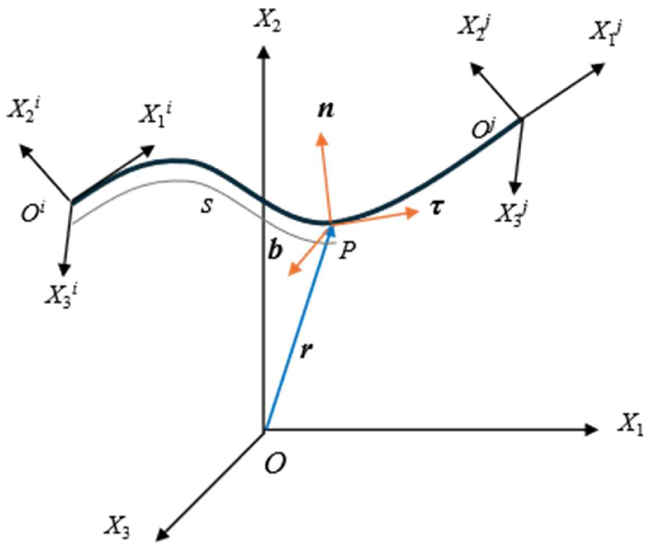
The influence of cross-sectional torsion and shear deformation of cables can be neglected in the present research owing to the large aspect ratios [23]. Hence, the bending and stretching deformations are described by the three-dimensional reduced beam model, which is illustrated in Figure 1.

By employing a two-point cubic Hermite interpolation scheme, the absolute position vector r in the global coordinate system is formulated as r = Sq. In this expression, S represents the shape function matrix, while q denotes the generalized nodal coordinates for element k. Specifically, q is a 12-dimensional vector that comprehensively captures the axial stretching and bending behaviors, which takes the form:

$${\mathit{q}}^k={[r_1^i r_2^i r_3^i \frac{\partial r_1^i}{\partial s} \frac{\partial r_2^i}{\partial s} \frac{\partial r_3^i}{\partial s} r_1^j r_2^j r_3^j \frac{\partial r_1^j}{\partial s} \frac{\partial r_2^j}{\partial s} \frac{\partial r_3^j}{\partial s}]}^T$$

(1)

where i and j represent nodes at the ends of the element. For each node, the first three components define the position vector in the global coordinate system, whereas the remaining three components define the slope vector, i.e., the first derivative of the position vector with respect to the material coordinate s measured along the undeformed cable centerline.

The external virtual work $W_e^k$ of element k is the product of the external force and the virtual displacement, which is expressed as:

$$\delta {\mathrm{W}}_e^k={\displaystyle {\displaystyle \underset{0}{\overset{L}{\int }}}{\mathit{f}}^T\delta {\mathit{r}}_p^{k}ds}=\left({\displaystyle {\displaystyle \underset{0}{\overset{L}{\int }}}{\mathit{f}}^T\cdot \frac{\partial \mathit{r}}{\partial \mathit{q}}ds}\right)\delta {\mathit{q}}^k={\mathit{Q}}_e^{k^T}\delta {\mathit{q}}^k$$

(2)

where ${\mathit{r}}_p^k$ is the vector of point P on element k, and f is the distributed external force acting on the cable element. The generalized external force vector of element k is expressed as

$${\mathit{Q}}_e^k={\mathit{Q}}_g^k+{\mathit{Q}}_b^k+{\mathit{Q}}_c^k+{\mathit{Q}}_h^k$$

(3)

where ${\mathit{Q}}_g^k$, ${\mathit{Q}}_b^k$, ${\mathit{Q}}_c^k$ and ${\mathit{Q}}_h^k$ denote the generalized forces associated with gravity, buoyancy, cable–seabed contact, and hydrodynamic loading, respectively.

The virtual work $W_k^i$ of the inertia force and the virtual work $W_k^s$ of the elastic force caused by deformation can be expressed as:

$$\delta W_k^i=\left({\ddot{\mathit{q}}}^{k^T}{\displaystyle {\displaystyle \underset{0}{\overset{L}{\int }}}\rho A{\mathit{S}}^T\mathit{S}ds}\right)\delta {\mathit{q}}^k={\left({\mathit{M}}^k{\ddot{q}}^k\right)}^T\delta {\mathit{q}}^k$$

(4)

$$\delta W_s^k=\left({\displaystyle {\displaystyle \underset{0}{\overset{L}{\int }}}EA}\epsilon {\displaystyle \frac{\partial \epsilon }{\partial \mathit{q}}}ds+{\displaystyle {\displaystyle \underset{0}{\overset{L}{\int }}}EI\kappa }{\displaystyle \frac{\partial \kappa }{\partial \mathit{q}}}ds\right)\delta {\mathit{q}}^k={\mathit{Q}}_s^{k^{\mathrm{T}}}\delta {\mathit{q}}^k$$

(5)

where ρ is the structural density, A is the cross-sectional area of the cable, L is the length of the element, E is the Young’s modulus of the cable, I is the moment of inertia of the cable section, M^k is the mass matrix of the unit, and ${\mathit{Q}}_s^k$ is the elastic force of the unit. In addition, ε and κ denote the Green strain and spatial point curvature.

The balance equation of the cable has been derived via element assembly

$${\displaystyle {\displaystyle \sum }_{k=1}^n}{\left({\mathit{M}}^k{\ddot{\mathit{q}}}^k+{\mathit{Q}}_s^k-{\mathit{Q}}_e^k\right)}^T \delta {\mathit{q}}^k={\left(\mathit{M}\ddot{\mathit{q}}+{\mathit{Q}}_s-{\mathit{Q}}_e\right)}^T \delta \mathit{q}=0$$

(6)

where M, Q_s, and Q_e are the mass matrix of the cable, the elastic force vector, and the external force vector, respectively.

2.2. External Loads

In this study, the cable is considered as a continuous and uniform tubular structure with no fluid inside. Considering drag, fluid inertia, and additional mass, the Morison equation is utilized in calculating the hydrodynamic forces,

$${\mathit{f}}_c={\displaystyle \frac{1}{2}}{\rho }_w{C}_{d}D{\mathit{U}}_n‖{\mathit{U}}_n‖+{\rho }_w{A}_0{C}_m\mathit{N}{\stackrel{.}{\mathit{v}}}_s-{\rho }_w{A}_0{C}_a\mathit{N}\stackrel{..}{\mathit{r}}$$

(7)

where C_m and C_a represent inertia and additional mass coefficients, D is the effective hydrodynamic diameter, ρ_w is the density of sea water, v_s and ${\dot{v}}_{\mathrm{s}}$ are fluid velocity and acceleration, and $\stackrel{.}{r}$ and $\stackrel{..}{r}$ are structural velocity and acceleration, respectively. N is a three-dimensional normal matrix, expressed as:

$$\mathit{N}={\mathit{I}}_{3\times 3}-{\displaystyle \frac{{\mathit{r}}^{\prime }{\mathit{r}}^{\prime \mathrm{T}}}{{\mathit{r}}^{\prime \mathrm{T}}{\mathit{r}}^{\prime }}}$$

(8)

where r’ = ∂r/∂s is the tangent vector of the cable centerline. The relative normal velocity between the fluid and the cable is expressed as

$${\mathit{U}}_n=\mathit{N}\left({\mathit{v}}_s-\dot{\mathit{r}}\right)$$

(9)

The cable–seabed interaction is decomposed into lateral and vertical components. The lateral seabed resistance is described using a Coulomb-friction-based bilinear model, in which the resistance first increases linearly with lateral displacement and then reaches a limiting friction force. The vertical seabed resistance is calculated using the Randolph–Quiggin model [22], which accounts for initial penetration, uplift suction, and repenetration during repeated cable–seabed contact. During the initial penetration stage, the vertical resistance is expressed as

$$P(z_p)={\displaystyle \frac{\xi }{1+\xi }}{P}_u(z_p)$$

(10)

$$\xi ={\displaystyle \frac{z_p{K}_{\max }}{D}}$$

(11)

where z_p is the penetration depth, K_max is the normalized maximum stiffness, and P_u(z_p) is the ultimate penetration resistance. The uplift and repenetration stages follow the hysteretic rules, allowing the nonlinear seabed memory effect and suction resistance near the touchdown zone to be represented in the time-domain analysis. For the sake of brevity, the details of nonlinear cable–seabed interactions are modeled can be found in Li et al. [21].

2.3. Damage Assessment Methods

Under cyclic loading, fatigue failure is a significant factor affecting the service life. In the present study, the S-N curve method, which describes the relationship between the fatigue strength S of the material and the number of stress cycles N during material failure, is combined with Miner’s linear cumulative damage theory [24], as expressed by:

$$N_i{=aS}_{\mathit{i}}^{-\mathit{m}}$$

(12)

where S_i is the ith stress range, N_i is the corresponding number of cycles to failure, and a and m are material parameters. The cumulative fatigue damage is then calculated as

$$D_f={\displaystyle \sum _{i=1}^n\frac{n_i}{N_i}}$$

(13)

where n_i is the number of cycles occurring at stress range S_i. Fatigue failure is assumed to occur when D_f reaches unity.

The wear failure of the cable on the TDZ induced by cable motion under complex flow field is investigated based on the Archard wear model [25],

$$V_w={\displaystyle \frac{{KF}_N{L}_f}{H}}$$

(14)

where V_w is the total wear volume, F_N denotes normal load, H is material hardness, L_f represents sliding distance, and K stands for wear coefficient. The dynamic wear equation is given by

$$V(t)={\displaystyle \frac{K}{H}}{\displaystyle {\int }_0^{t}p}(\mathsf{\tau })\times v(\mathsf{\tau })d\mathsf{\tau }$$

(15)

where p(τ) denotes instantaneous contact pressure and v(τ) represents instantaneous sliding velocity.

3. Numerical Validation

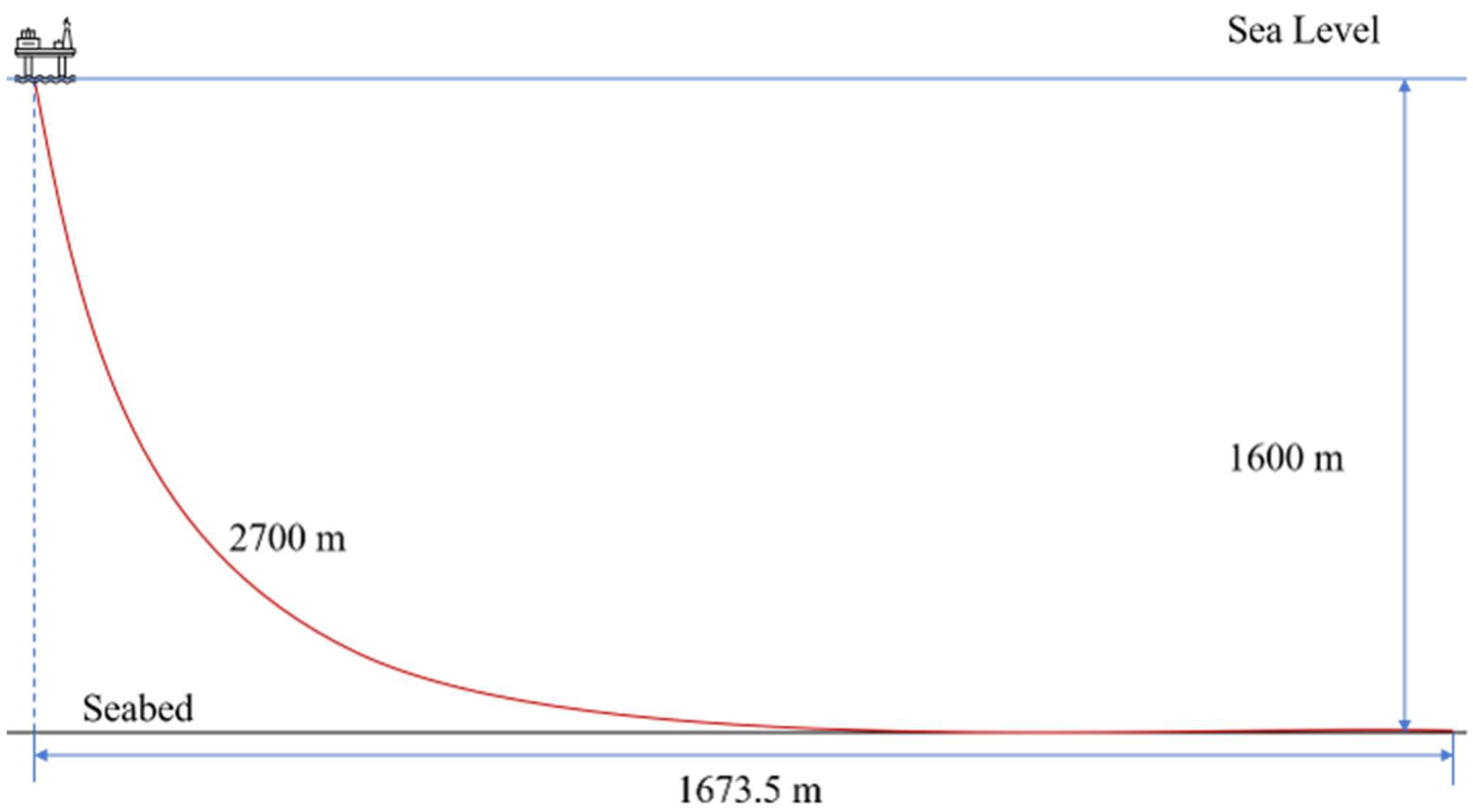
To validate the accuracy and reliability of the proposed ANCF-based cable model, the benchmark catenary riser case reported by Yu et al. [26] is reproduced. Although this benchmark case was originally developed for a deep-water riser system, its catenary configuration and nonlinear flexible structural characteristics are highly representative of suspended marine cables, making it suitable for validating the present formulation. Figure 2 presents the geometric configuration of the benchmark model, and

Table 1. Parameters of the riser model [26].

Parameter	Value	Parameter	Value
Length	2700 m	Bending stiffness	58,648 kNm2
External diameter	0.324 m	Dry mass	197.428 kg/m
Internal diameter	0.270 m	Shear strength gradient	1.5 kPa/m
Axial stiffness	528.2 MN	Mudline shear strength	0.6 kPa

summarizes the corresponding geometric parameters, structural properties, boundary conditions, and nonlinear seabed parameters.

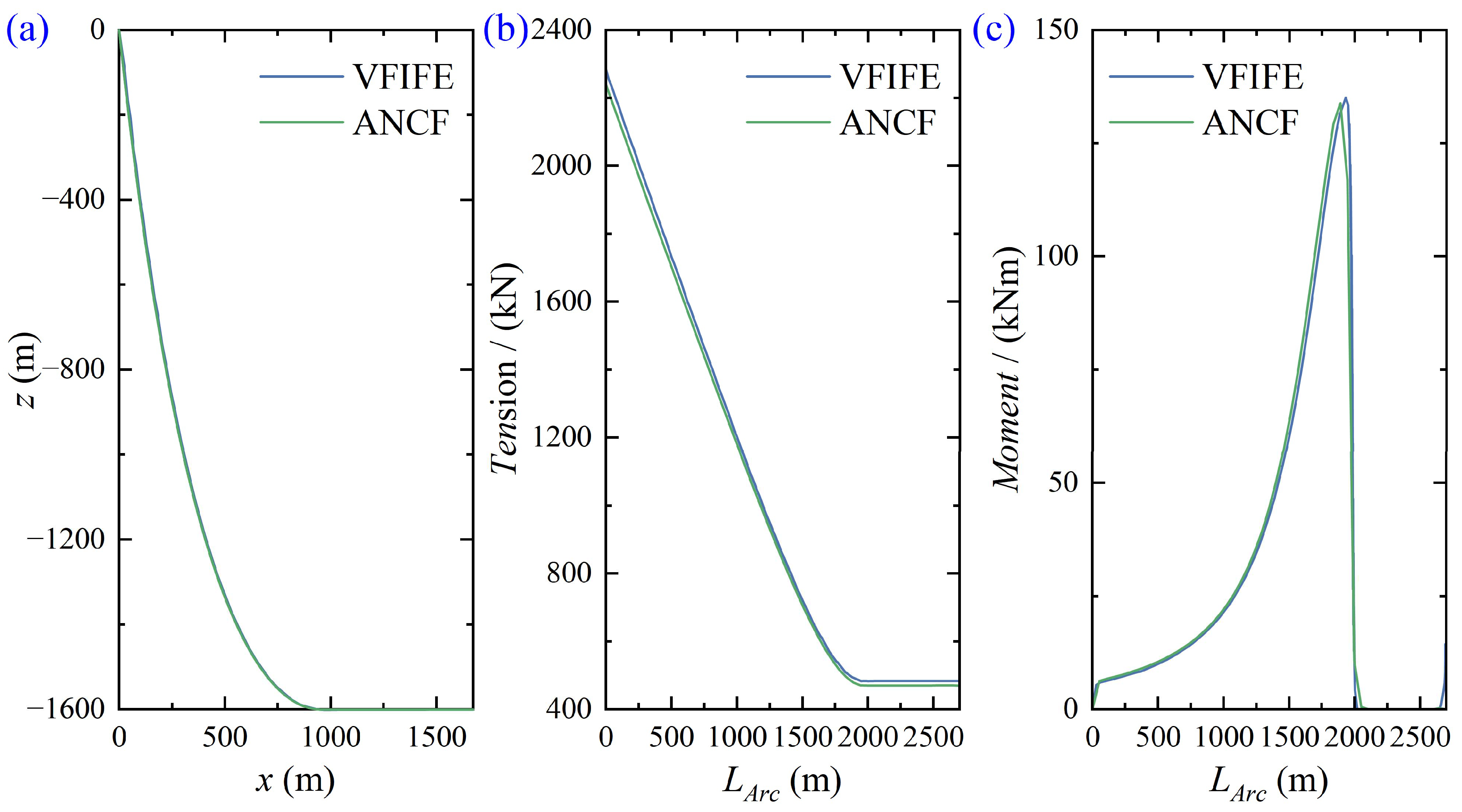
As shown in Figure 3, the ANCF predictions show good agreement with the VFIFE results in terms of the riser configuration, top tension, and bending moment. The relative differences in the maximum top tension and bending moment are only 2.0% and 0.9%, respectively. These comparisons demonstrate that the present ANCF model can accurately capture the global dynamic response of suspended catenary flexible structures.

4. Problem Description

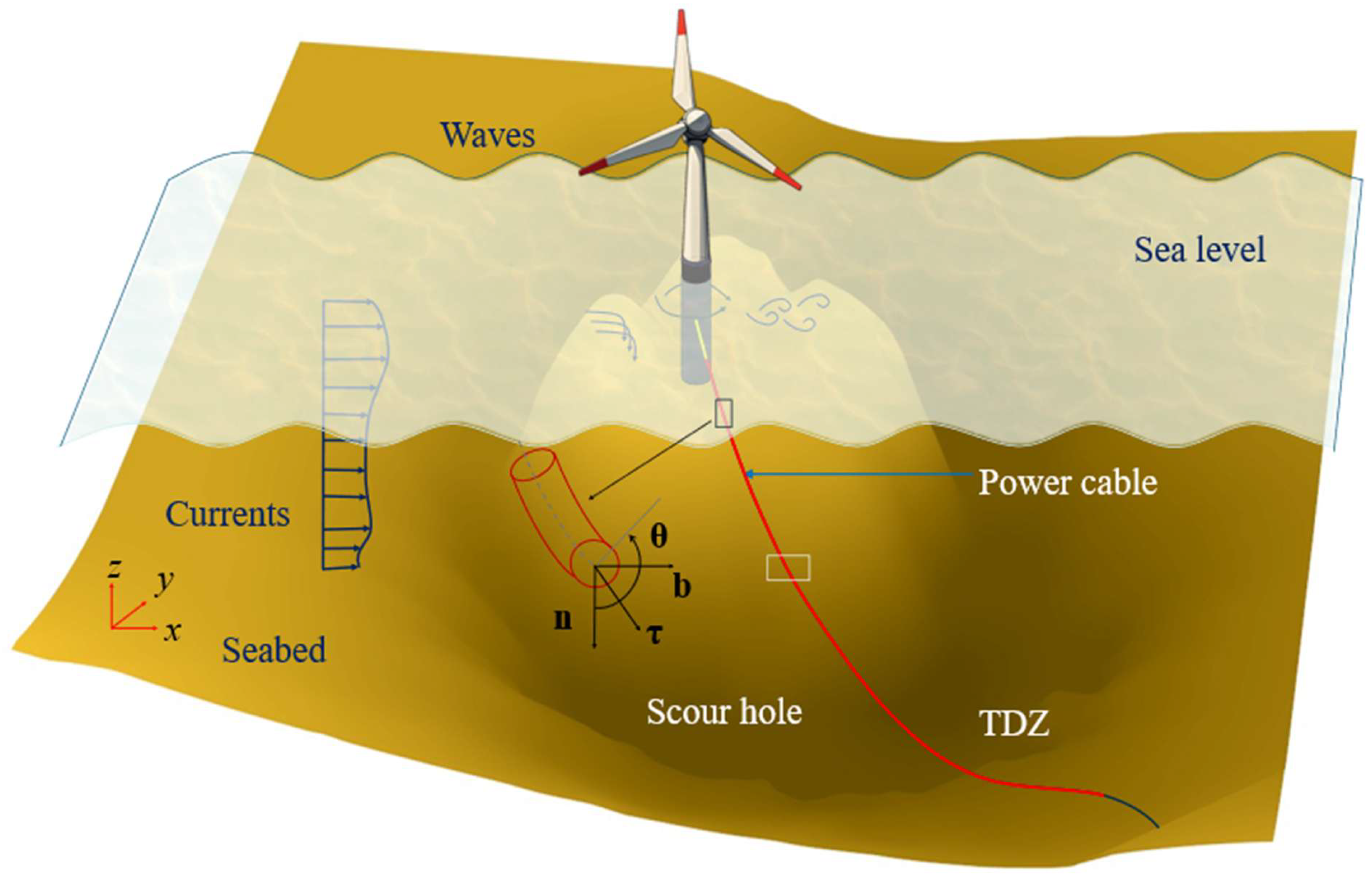
The configuration of the cable system investigated in the present study is indicated in Figure 4. A power cable extending from the pile of an in-service offshore wind turbine, which is located in the South China Sea, is investigated. A global coordinate system is defined with its origin at the top center of the pile foundation, where the $x$-, $y$-, and $z$-axes point eastward, northward, and vertically upward, respectively. The submergence depth of the top end of the cable is 9.0 m, while that of its bottom end is 11.7 m. Unlike the idealized flat-seabed assumption commonly adopted in cable-response analyses, the spatially varying and irregular seabed profile along the cable route is explicitly incorporated into the geometric and cable–seabed contact models. In the present study, seabed variation refers to the spatial variation in seabed elevation rather than temporal seabed evolution, and the prescribed seabed profile remains unchanged during the dynamic analysis. In the horizontal plane, the cable is oriented at an azimuth of 255°, while the line connecting its upper endpoint to the pile center has an azimuth of 250°. The structural properties of the cable and the environmental parameters of the operational sea area are summarized in

Table 2. Parameters of cable and ocean environment.

Parameter	Value	Parameter	Value
Pile radius	3.4 m	Axial stiffness	290 MN
Density of sea water	1025 kg/m3	Bending stiffness	4.5 kNm2
Density of cable	2782.97 kg/m3	Seabed friction coefficient	0.5
Cable length	25.2 m	Allowable bending radius	4 m
Cable diameter	0.1456 m	sg	1.116 kPa/m
Added mass coefficient	1.0	ks	46.7 kN/m3
Drag coefficient	1.2

.

The current velocity cannot be accurately described by simple linear or exponential models due to the seabed terrain and flow around the pile in practice. Therefore, the localized flow field is simulated by using FluidX3D, a computational fluid dynamics (CFD) solver based on the Lattice Boltzmann Method (LBM). The underlying numerical implementation of FluidX3D has been benchmarked by Lehmann et al. [27], while its principal configurations for the present site-specific simulation are summarized in

Table 3. Parameters of the CFD model.

Parameter	Value
Computational domain	80 m × 80 m × 14 m
Grid resolution	0.1 m
Pile boundary condition	No-slip wall
Inflow condition	Exponential shear profile
Seabed boundary condition	Stationary rough wall
Top boundary condition	Free surface
Lateral boundary conditions	Periodic boundaries

.

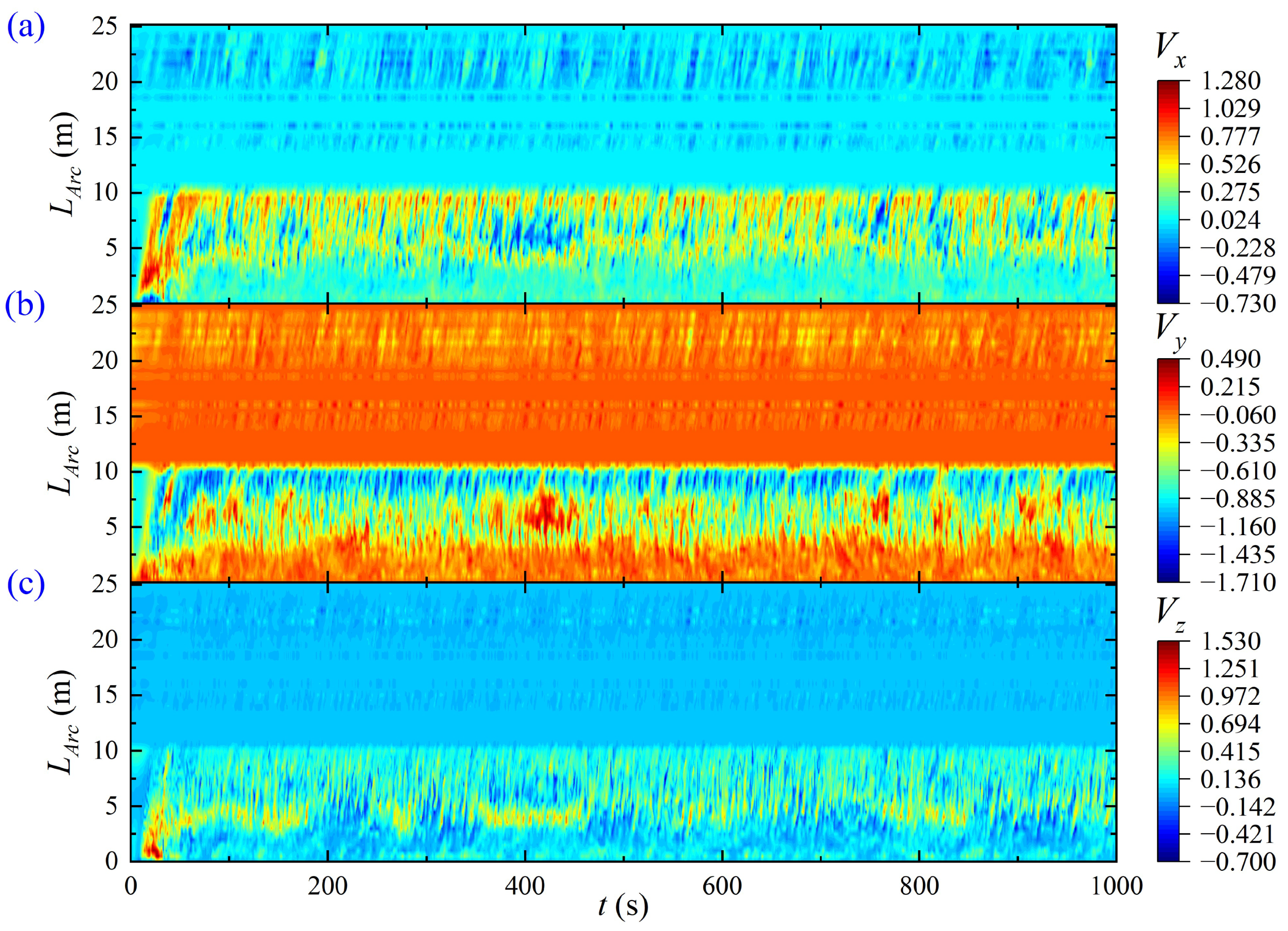
The velocity results obtained from the CFD model are depicted in Figure 5. Specifically, the velocity components in the x-, y-, and z-directions fluctuate within the ranges of −0.730 to 1.280 m/s, −1.710 to 0.490 m/s, and −0.770 to 1.530 m/s, respectively. Notably, the velocity magnitude remains relatively low around the pile foundation within the arc length L_Arc from 0 to 10 m. In contrast, pronounced oscillations are observed in the middle and rear portions of the suspended span. This localized amplification can probably be attributed to the horseshoe vortices generated by the interaction between the incident current and the seabed. In the present study, the simulation cases are designed as listed in

Table 4. Summary of simulation cases.

	Case	Incident Angle (°)	Wave Height (m)	Wave Period (s)	Tide Level (m)
Typical Case	1	13	2.54	8.8	0
Pure Current	2	13	-	0
Incident Angle	3	0	2.54	8.8	0
	4	25	2.54	8.8	0
	5	40	2.54	8.8	0
	6	13	5.02	12.6	5.65
Return Period	7	13	4.49	11.5	5.47
	8	13	3.83	9.4	4.77
	9	13	3.23	8.3	4.53
	10	13	2.79	11.8	−0.43
	11	13	2.74	10.8	−0.34
	12	13	2.39	7.8	0.09

.

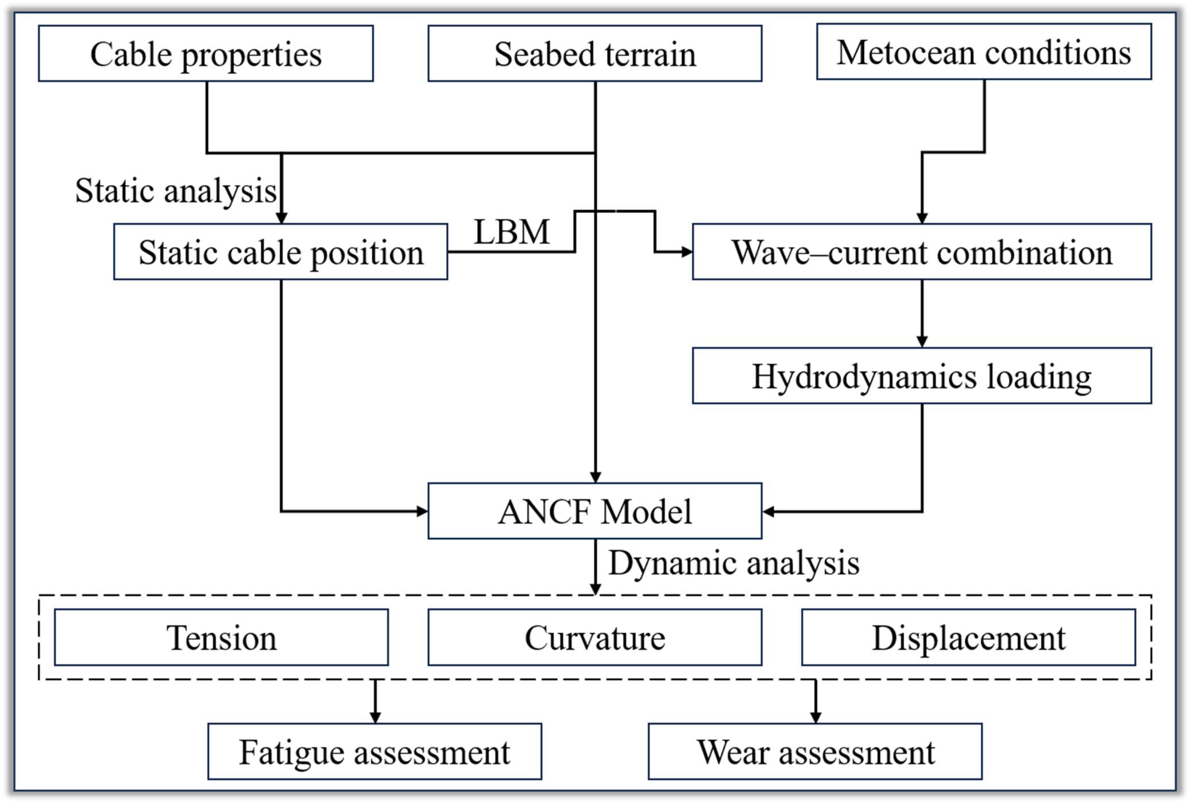
The overall computational framework adopted in this study is illustrated in Figure 6. The cable properties and irregular seabed terrain are first incorporated into the static equilibrium analysis to determine the initial cable configuration and contact state. The local current field is then calculated using the LBM, while the irregular waves are generated from the JONSWAP spectrum. The combined wave–current conditions are used to calculate the hydrodynamic loading and time-domain cable response. Finally, the resulting structural-response and contact histories are used for fatigue and wear assessments.

5. Characteristics of Dynamic Response

5.1. Response Characteristics Under the Typical Case

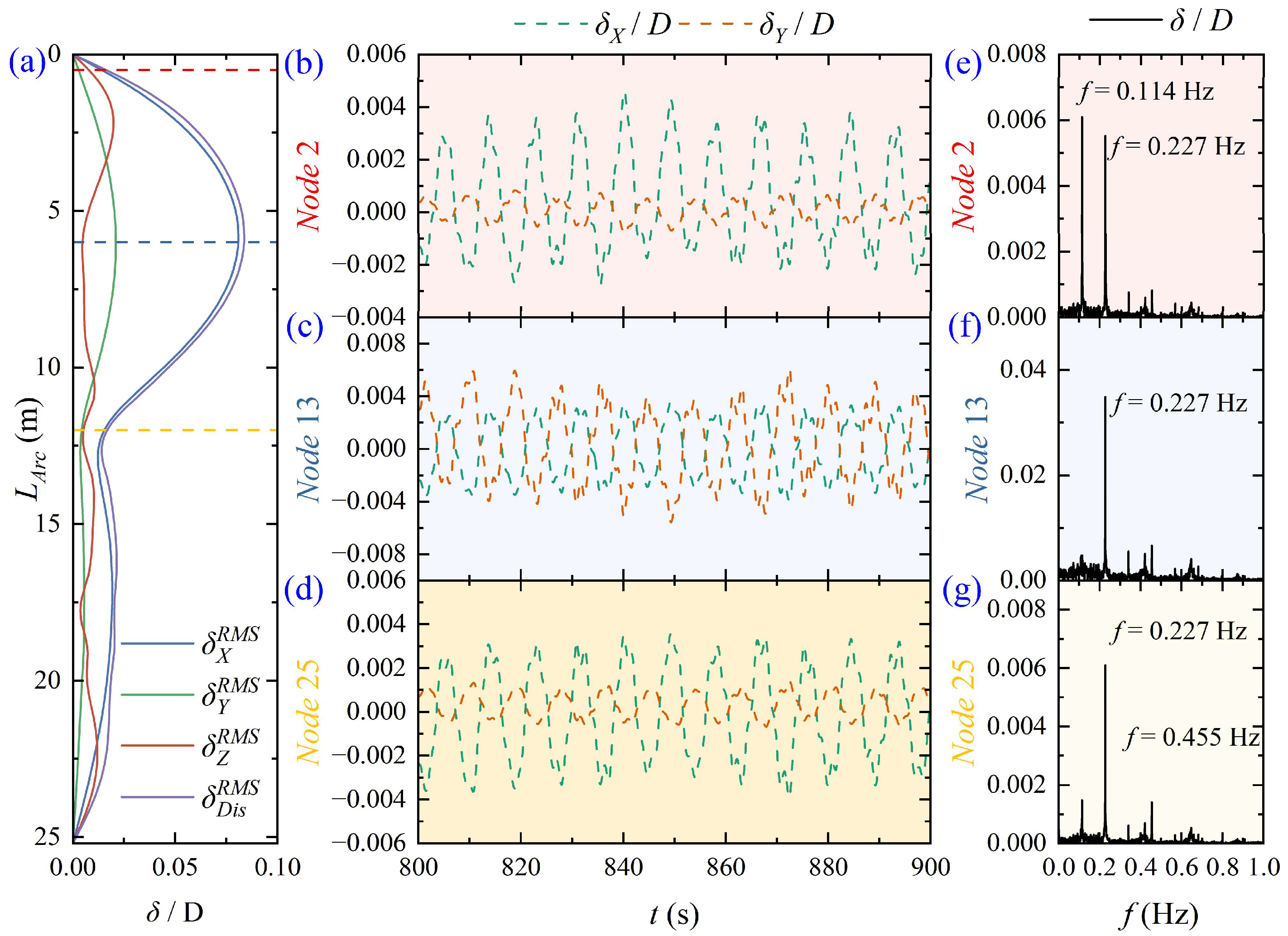
The wave condition Case 1 at the incident angle of 13° is selected as the typical case, considering the actual wave and current conditions. It is illustrated in Figure 7a that the response along the arc length of the cable exhibits pronounced non-uniformity under the combination of waves and flows. The x-displacement is the dominant component of the cable displacement, with the maximum dimensionless displacement of 0.0836, occurring at the arc length L_Arc = 6 m. In order to further examine the local dynamic characteristics, three representative nodes are selected from the near-pile region, the middle of the suspended span, and the TDZ, respectively. The time histories of displacement and spectra obtained by fast Fourier transform (FFT) are compared in Figure 7b–g. The displacement response of Node 2 near the pile is relatively small, with the dominant frequency at f = 0.114 Hz, which is consistent with the dominant frequency of the wave in the typical case. In contrast, the dominant frequencies of Nodes 13 and 25 shift to f = 0.227 Hz. Meanwhile, it is observed that some high-frequency components occur at f = 0.455 Hz.

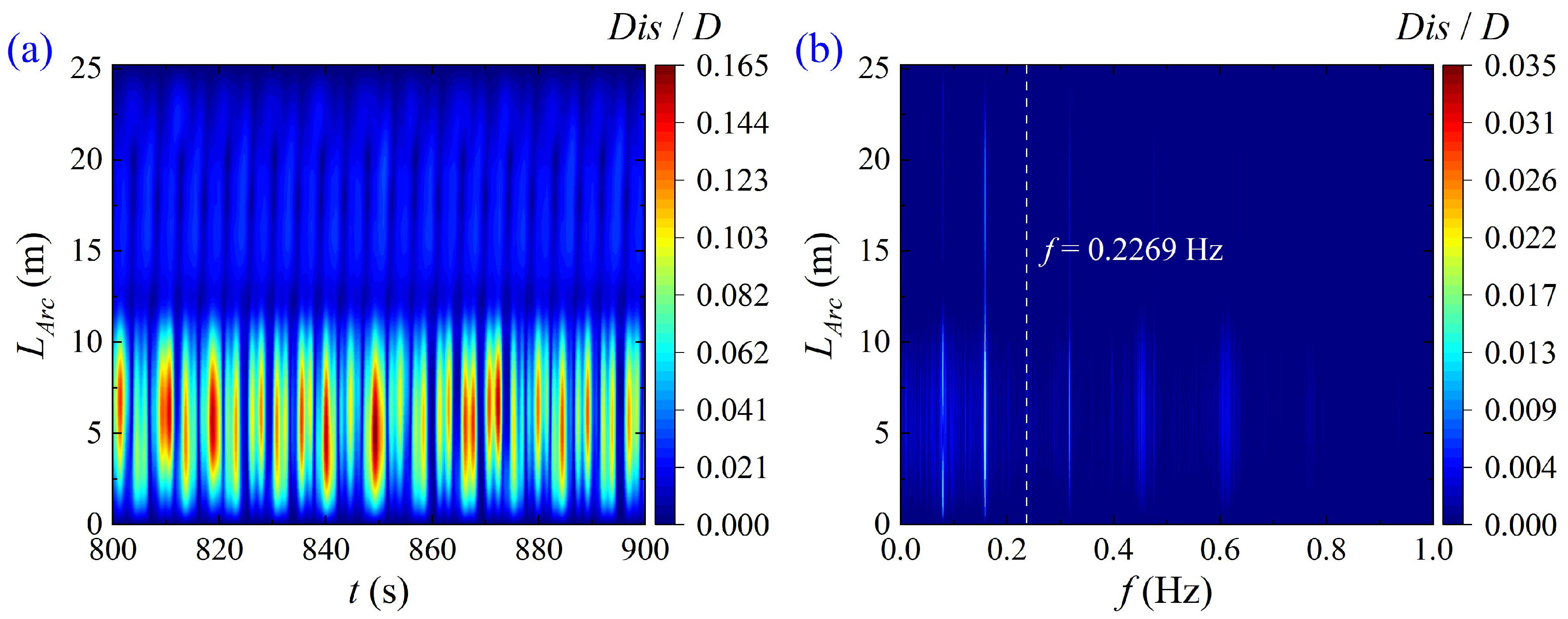
The displacement histories along the cable are shown in Figure 8a, indicating that the displacement response is spatially concentrated. Large displacement mainly occurs in the suspended span, particularly in the range of L_Arc = 3~10 m. The displacement amplitude decreases significantly near the TDZ, indicating the restraining effect of seabed interaction. Figure 8b further shows that the dominant frequency of the displacement response is concentrated at f = 0.2269 Hz, while no evident separation of dominant frequencies or local frequency shift is observed in the frequency-domain results.

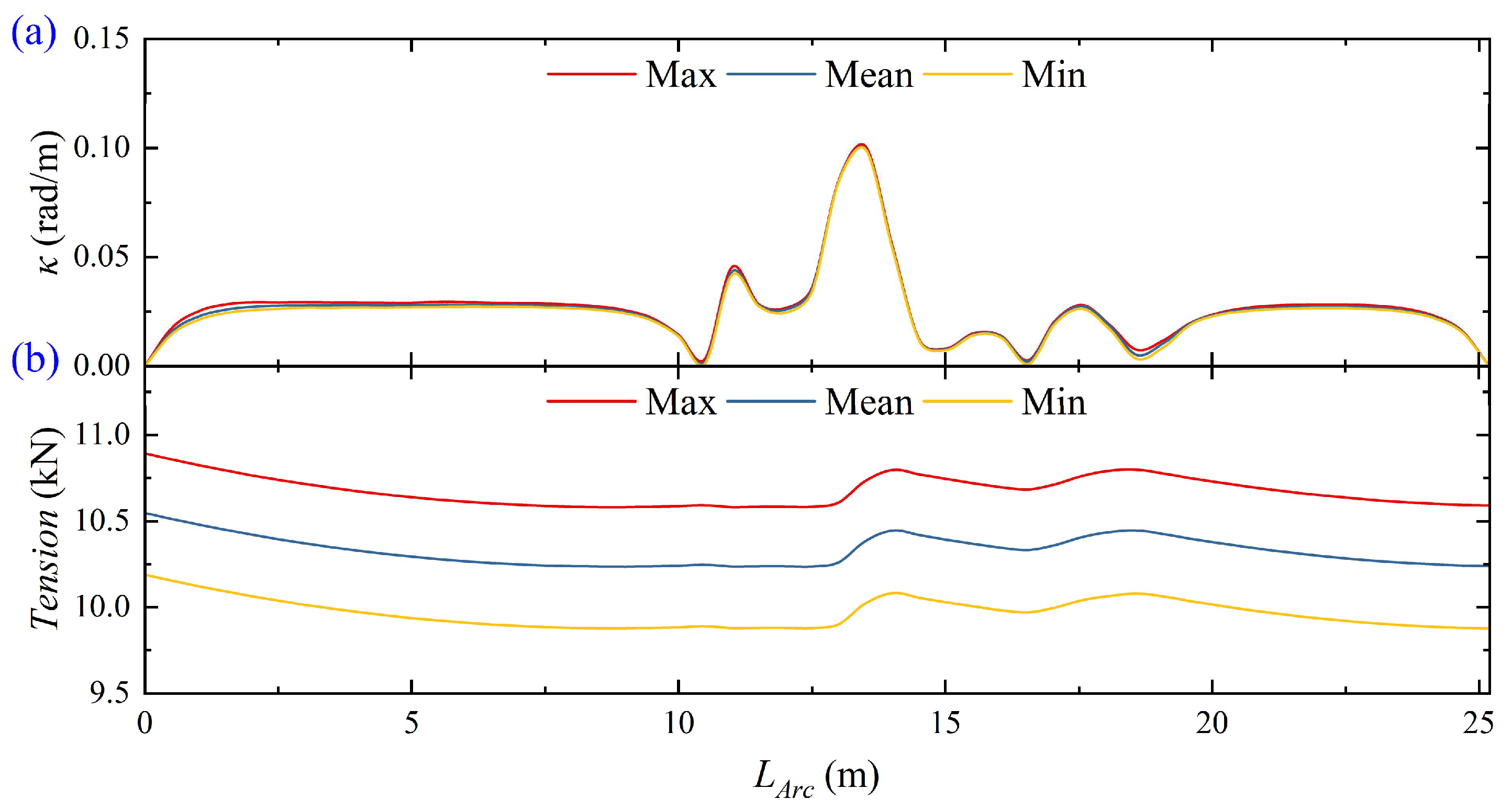
The statistical distributions of cable curvature and tension are presented in Figure 9. The cable curvature exhibits significant fluctuations within the range of L_Arc = 10~20 m, and reaches a peak value of 0.10 rad/m at L_Arc = 13.5 m. The cable tension generally decreases along the arc length, but two local peaks appear at L_Arc = 14 m and L_Arc = 18 m. These locations are broadly consistent with the regions where notable curvature fluctuations occur, indicating that local bending deformation from the cable–seabed interaction can induce a redistribution of axial force along the cable.

5.2. Effects of Wave Intensity

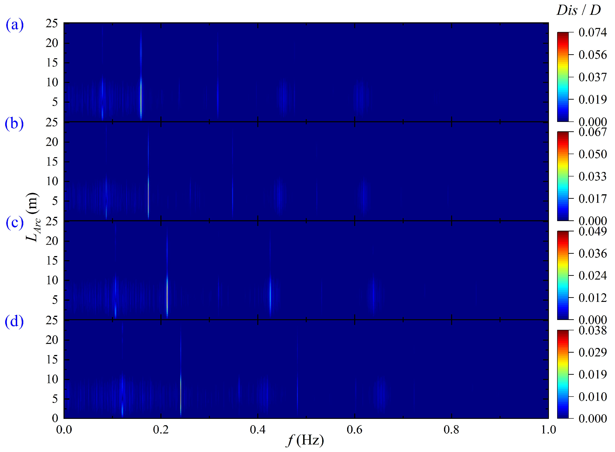
The dynamic response of the suspended export cable is further analyzed under wave conditions with different return periods, corresponding to Cases 6–9. The frequency-domain results along the arc length are presented in Figure 10. It is observed that the amplitude of the dimensionless FFT response increases from 0.038 to 0.074 with longer return periods. The dominant frequency of displacement is approximately twice the wave frequency, with no evident frequency shift observed. Meanwhile, the high-amplitude region is mainly located in the suspended span, and its spatial extent does not shift noticeably across the cases considered in the present study.

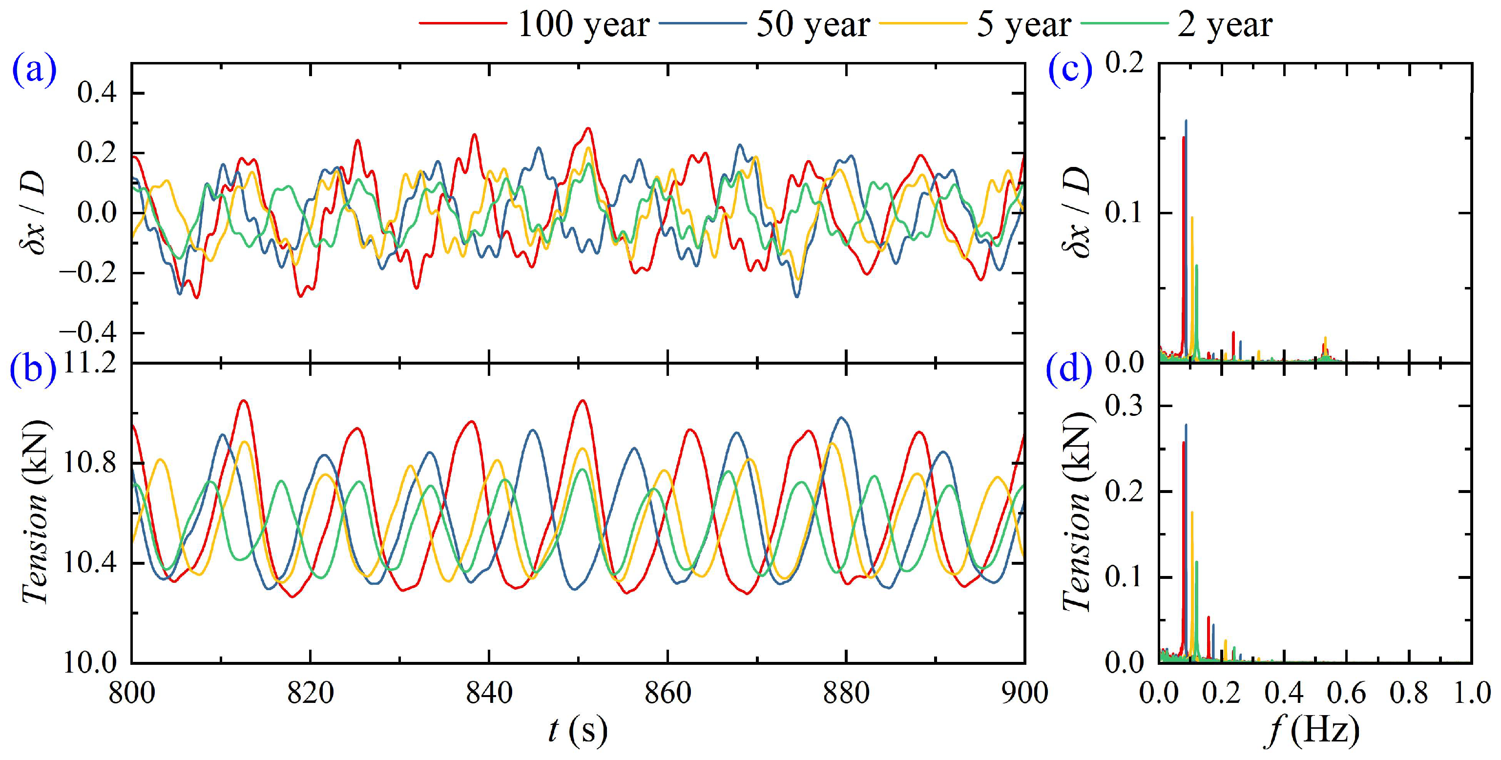
Based on the global displacement spectra discussed above, Figure 11 further compares the time histories and FFT spectra of the x-direction displacement and tension under different return-period conditions. The x-direction displacement oscillates around the equilibrium position, with its dominant frequency located near the wave frequency. In comparison, the tension response exhibits a clearer periodicity. It is worth noting that the spectral amplitude of the tension response is mainly concentrated around the low-frequency dominant peak, while no local high-frequency peak is observed near f = 0.52 Hz, in contrast to the x-displacement response. This result indicates that the tension response is relatively insensitive to local high-frequency disturbances.

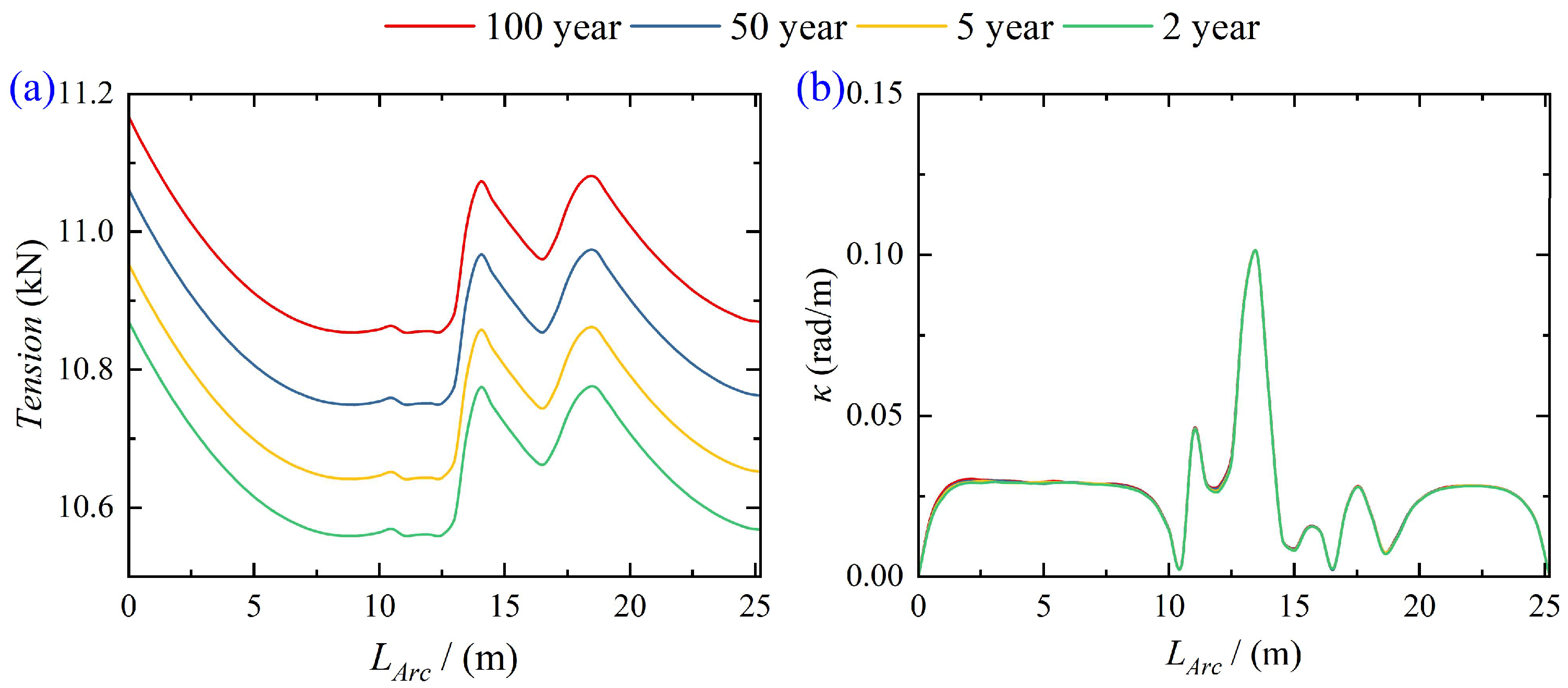
The statistical distributions of tension and curvature under different cases are shown in Figure 12. The maximum tension increases from 10.87 kN under the 2-year case to 11.17 kN under the 100-year case as the return period increases. However, the distribution pattern of tension along the cable remains almost unchanged, suggesting that the increase in wave intensity primarily elevates the overall axial force level rather than altering its spatial distribution. Meanwhile, the curvature distributions under different return periods almost overlap, with the maximum curvature approximately 0.10 rad/m.

5.3. Effects of the Wave–Current Incidence Angle

Four representative incident angles, 0°, 13°, 25°, and 40°, were selected to characterize the displacement response under progressively increasing directional deviations of the combined wave–current loading. The 0° case represents aligned loading, 13° represents the reference loading direction adopted in this study, and 25° and 40° represent moderate and relatively large oblique-incidence conditions, respectively, within the range considered in this study.

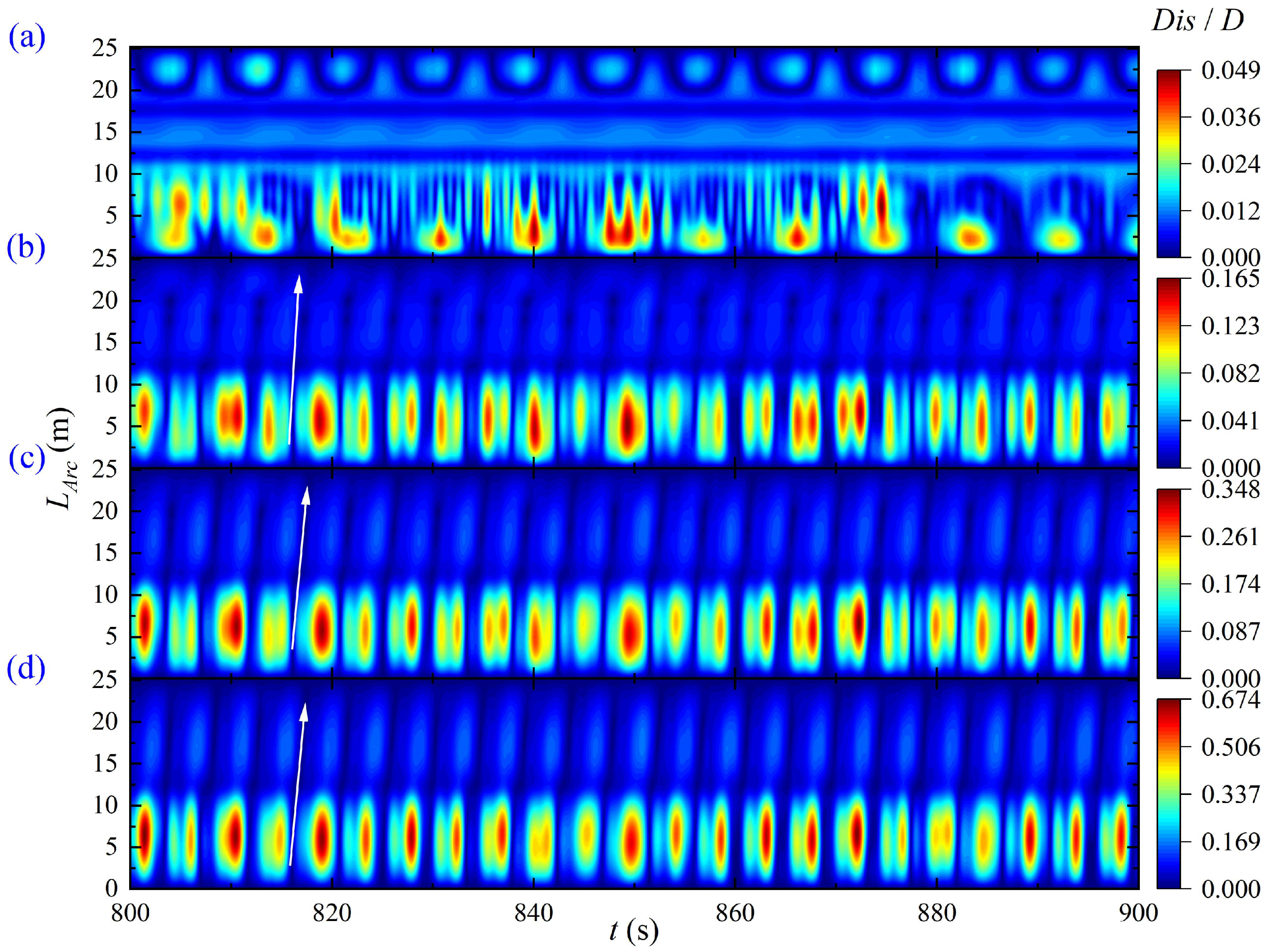
The time-histories of the cable displacement at t = 800~900 s under different incident angles, corresponding to Cases 1 and Case 3–5, are illustrated in Figure 13. The results show the pronounced effects of incident angle on cable displacement. Under the 0° condition, the displacement response is relatively weak, and the high-amplitude regions are confined to several local arc-length ranges. No clear continuous inclined band is observed in the time–arc length plane, suggesting that the cable response is more localized under this condition. Since the continuous propagation along the arc length is not prominent, the cable displacement under this condition mainly manifests as localized forced vibration. As the incident angle increases, the cable displacement becomes much stronger, and relatively continuous periodic high-amplitude bands are formed near the suspended area. These bands show an inclined distribution in the time–arc length plane, suggesting the existence of phase differences and propagation characteristics along the cable.

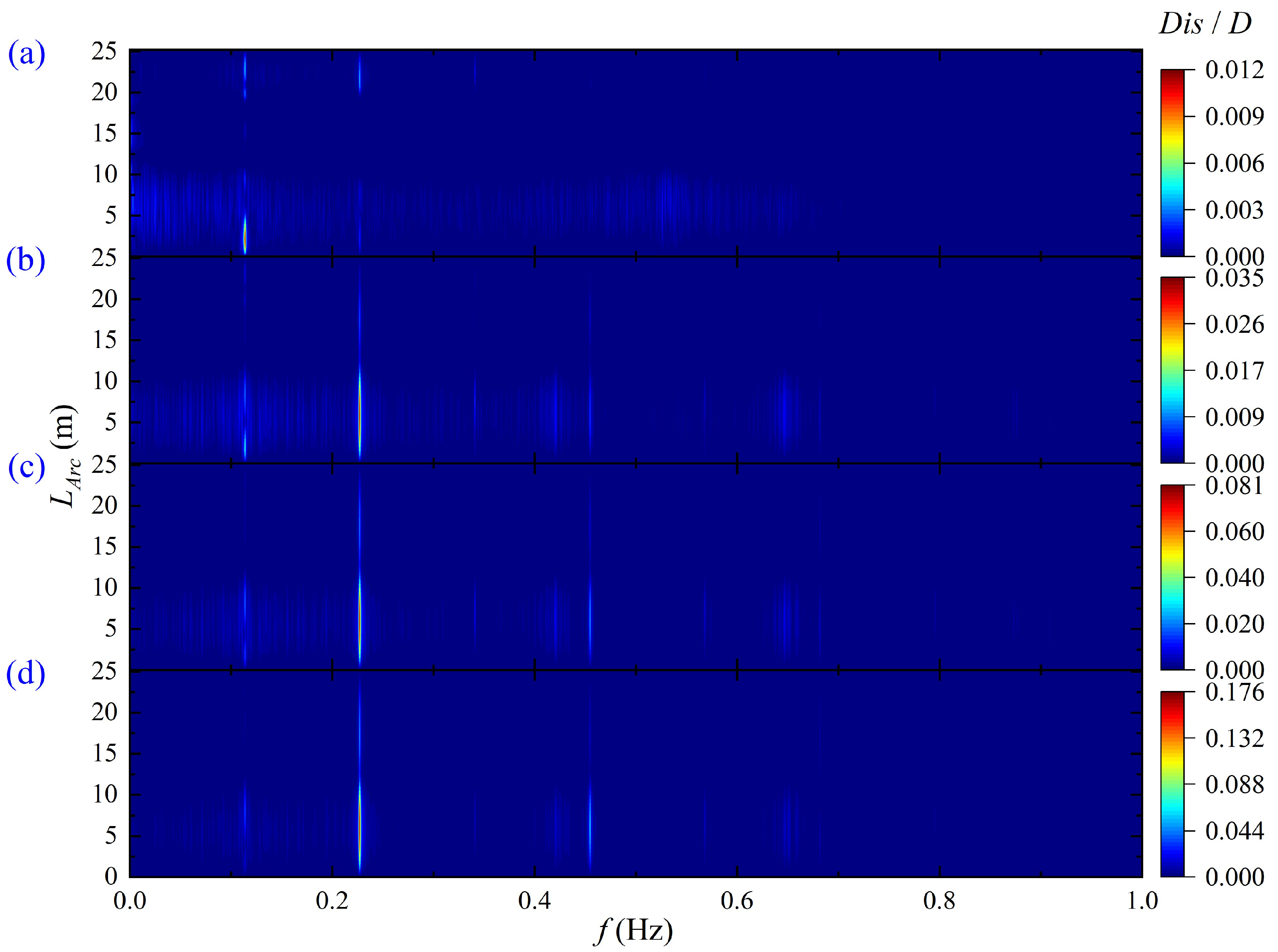
Figure 14 further reveals the frequency characteristics of the cable displacement under different wave–current incident angles. When the wave–current angle is 0°, the dominant frequency of the total displacement response is mainly concentrated near f = 0.114 Hz, which is consistent with the dominant wave frequency. In addition, a distinct low-amplitude spectral band can be observed in the middle section of the cable, indicating that the displacement response in this region is suppressed. When the wave–current angle increases to 13°, 25°, and 40°, the dominant frequency of the cable displacement spectra shifts to approximately f = 0.227 Hz. Meanwhile, both low-frequency and high-frequency components become more pronounced within the suspended span, indicating a more complex frequency composition of the suspended-span motion under larger wave–current angles.

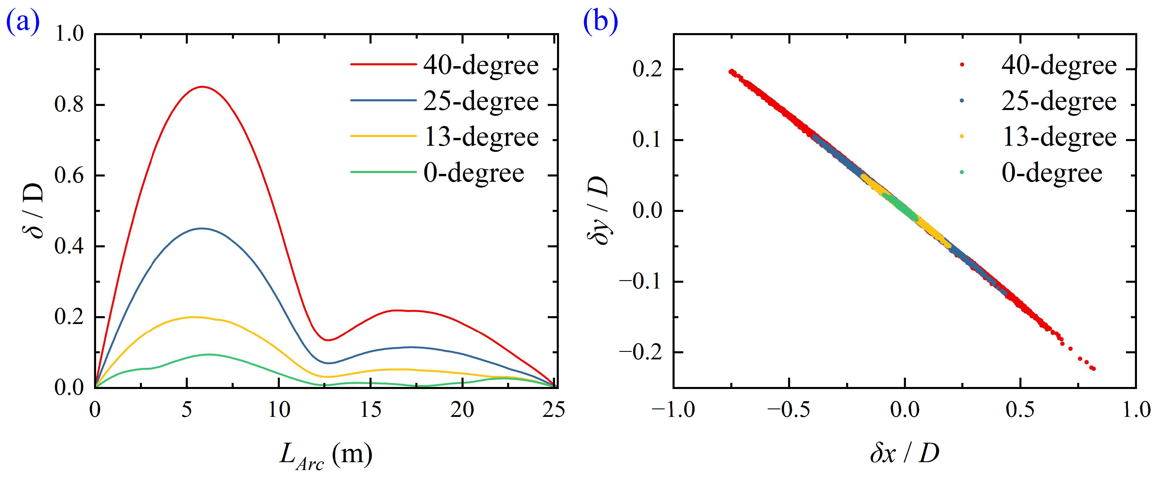
Statistical distributions of cable displacement and the horizontal-plane motion trajectories under different wave–current incident angles are presented in Figure 15. A clear turning point appears in the displacement curve near the transition from the suspended span to the TDZ. Compared with the non-zero angle cases, the 0° case exhibits a smaller displacement amplitude, and the peak values along the cable are more scattered. Figure 15b shows the horizontal-plane trajectory at the location where the maximum displacement occurs. It is observed that the displacement trajectories under different wave–current incident angles are generally aligned in the same direction, rather than rotating with the change in wave–current angle. The above phenomenon suggests that, under the present conditions, the wave–current angle mainly changes the displacement amplitude.

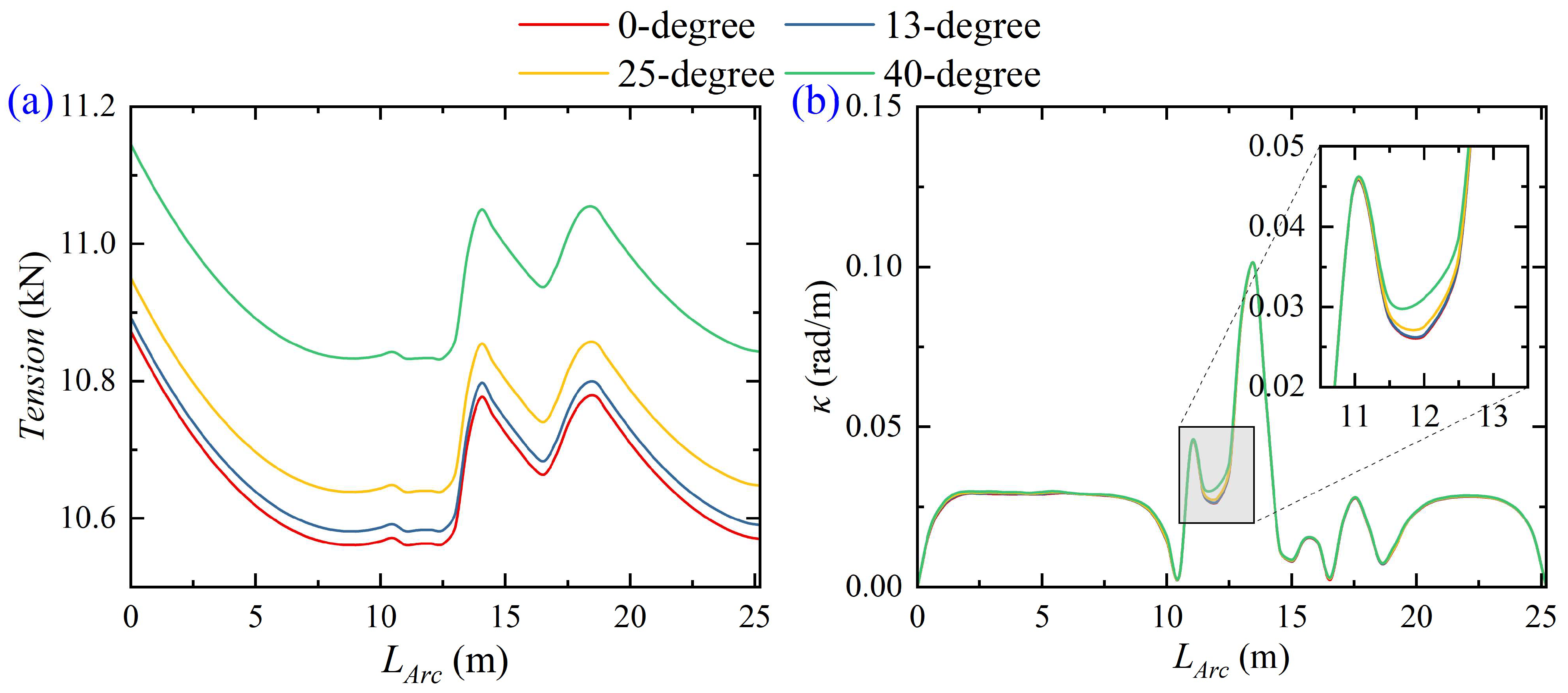
Figure 16 represents the statistical results of cable tension and curvature along the arc length. As the wave–current angle increases, the overall cable tension increases. However, the tension distribution shows a generally consistent pattern, with no obvious shift in the local peak locations. This indicates that the wave–current angle mainly increases the overall tension level of the cable, rather than significantly altering the primary load-bearing locations. In contrast, the curvature is more sensitive to changes in the wave–current angle, especially in the transition region from the suspended span to the TDZ. Within the range of L_Arc = 11~13 m, the curvature fluctuations become more pronounced as the wave–current angle increases, indicating that the local bending deformation in this region is enhanced. In other regions, however, the curvature distributions under different angles show only minor difference.

6. Cable Damage Assessment

6.1. Structural Strength of the Cable

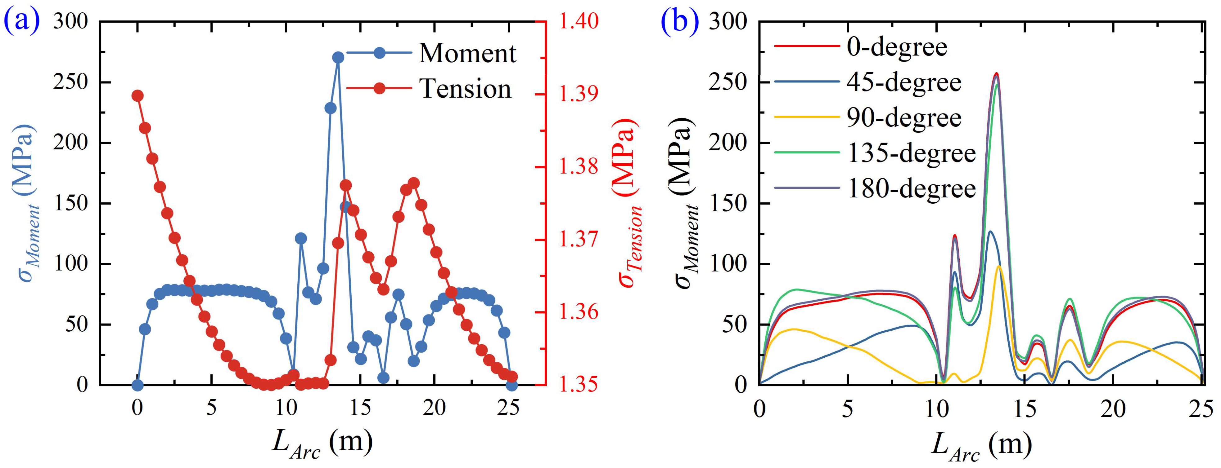
The strength verification is further conducted based on the dynamic response of the cable. In the present study, the ultimate stress of the cable material is taken as σ_s = 450 MPa, and the safety factor is set to 1.5. Therefore, the allowable stress is determined as 300 MPa. As shown in Figure 17a, the axial stress distribution along the cable follows the variation trend of cable tension, reaching a maximum value of 1.389 MPa. The bending stress increases significantly in the transition region from the suspended span to the TDZ, with a maximum value of 270.67 MPa. This result demonstrates that the cable stress is mainly governed by local bending deformation, making the transition region critical for the strength verification. Figure 17b further compares the combined stress distributions at different circumferential angular positions of the cable cross-section. The stress peaks at the 0°, 135°, and 180° positions are relatively large, with the maximum value approaching 253.5 MPa. In contrast, the maximum stresses at the 45° and 90° positions are significantly lower, both remaining below 150 MPa, indicating that these circumferential positions are relatively safe.

Table 5. Maximum stress under extreme conditions.

Case	Maximum Stress/MPa	Case	Maximum Stress/MPa	Case	Maximum Stress/MPa
1	273.27	5	273.32	9	273.30
2	273.30	6	273.34	10	273.32
3	273.31	7	273.33	11	273.31
4	273.31	8	273.31	12	273.30

summarizes the maximum stresses under all conditions. The results show that all stress values remain below the allowable stress of 300 MPa. Therefore, within the range of extreme sea states considered in this study, the cable satisfies the structural strength requirement, and no instantaneous overstress failure is expected.

6.2. Fatigue Damage of the Cable

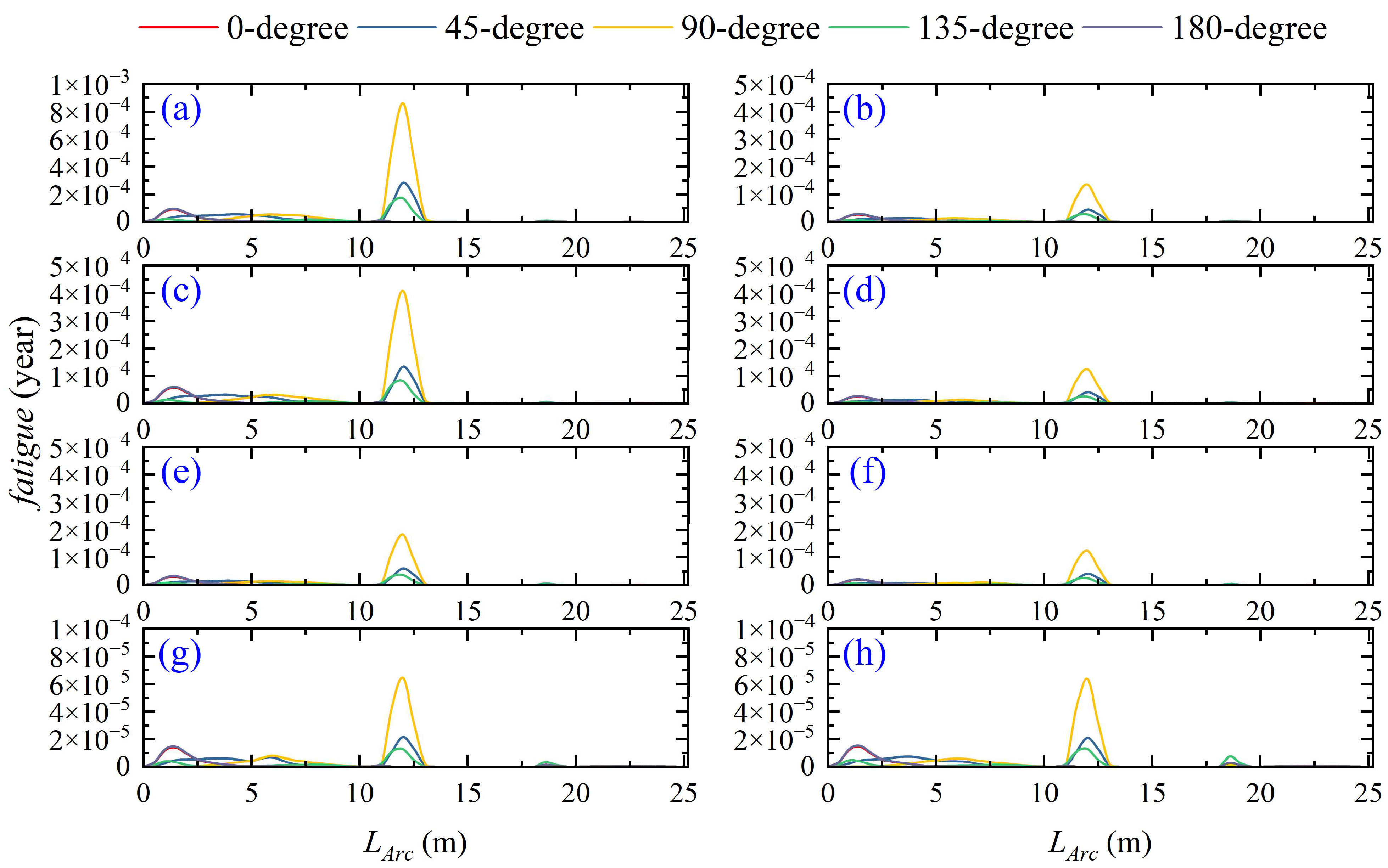
Figure 18 shows the fatigue damage distributions along the cable under different wave return periods and tide levels. The left column corresponds to Cases 6–9, while the right column corresponds to Case 1 and Cases 10–12. The fatigue damage becomes more pronounced under longer wave return periods, with higher damage levels observed under the high-water-level condition than under the low-water-level condition. The results imply that both wave intensity and water level affect the cyclic stress range of the cable. From the perspective of circumferential position, the fatigue damage at the 90° position is significantly higher than that at the other angular positions. This suggests that this position experiences stronger cyclic stress and represents the most unfavorable circumferential position in the fatigue assessment. In contrast, the damage levels at the other circumferential positions are relatively low, indicating that the fatigue damage is clearly non-uniform around the cable cross-section.

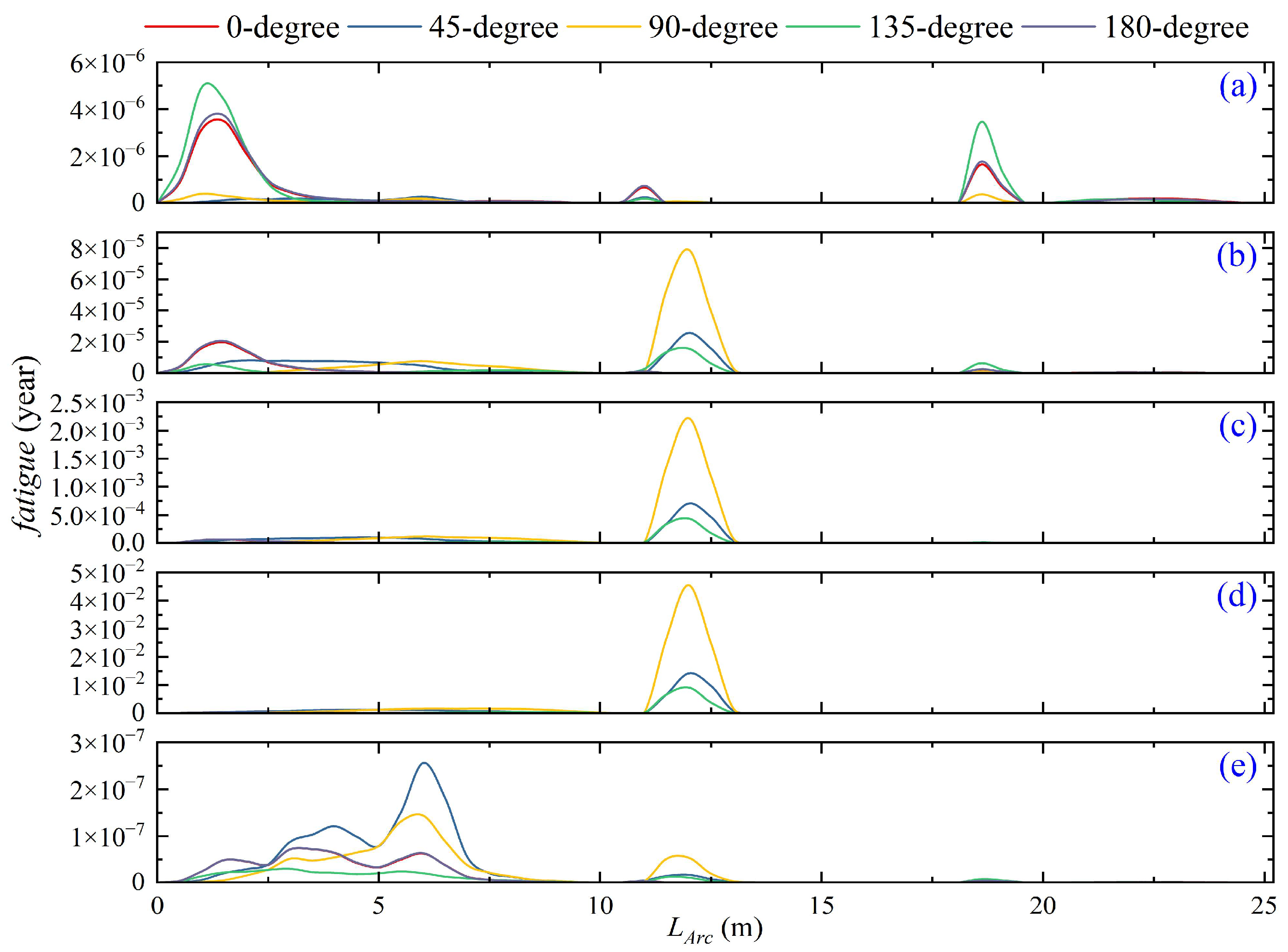
Figure 19 indicates that the incident angle alters both the fatigue hotspot locations and the most unfavorable circumferential angles of the power cable. Under the 0° incident angle, the fatigue damage remains relatively low, peaking at the 135° circumferential position. In contrast, non-zero angles shift the maximum fatigue damage to the 90° circumferential position. The damage concentrates within the suspended-to-touchdown transition zone, located in the range of L_Arc = 11~13 m. Notably, a local fatigue peak persists at the suspended segment under the 13° condition, reflecting the transitional characteristics of fatigue hotspots at small incident angles. Under the pure current condition shown in Figure 19e, the overall fatigue damage is limited due to the absence of waves. The maximum damage is low and occurs at the 45° circumferential position along the forward section of the suspended segment.

6.3. Wear Damage of the Cable

The assessment of local wear damage in the TDZ is further carried out based on the dynamic responses of the cable obtained under various wave–current conditions. The wear analysis is based on the Archard wear model. A finite element contact wear model is established in ANSYS Workbench 2025 R2 to simulate the wear evolution of the cable’s outer surface under different displacement conditions.

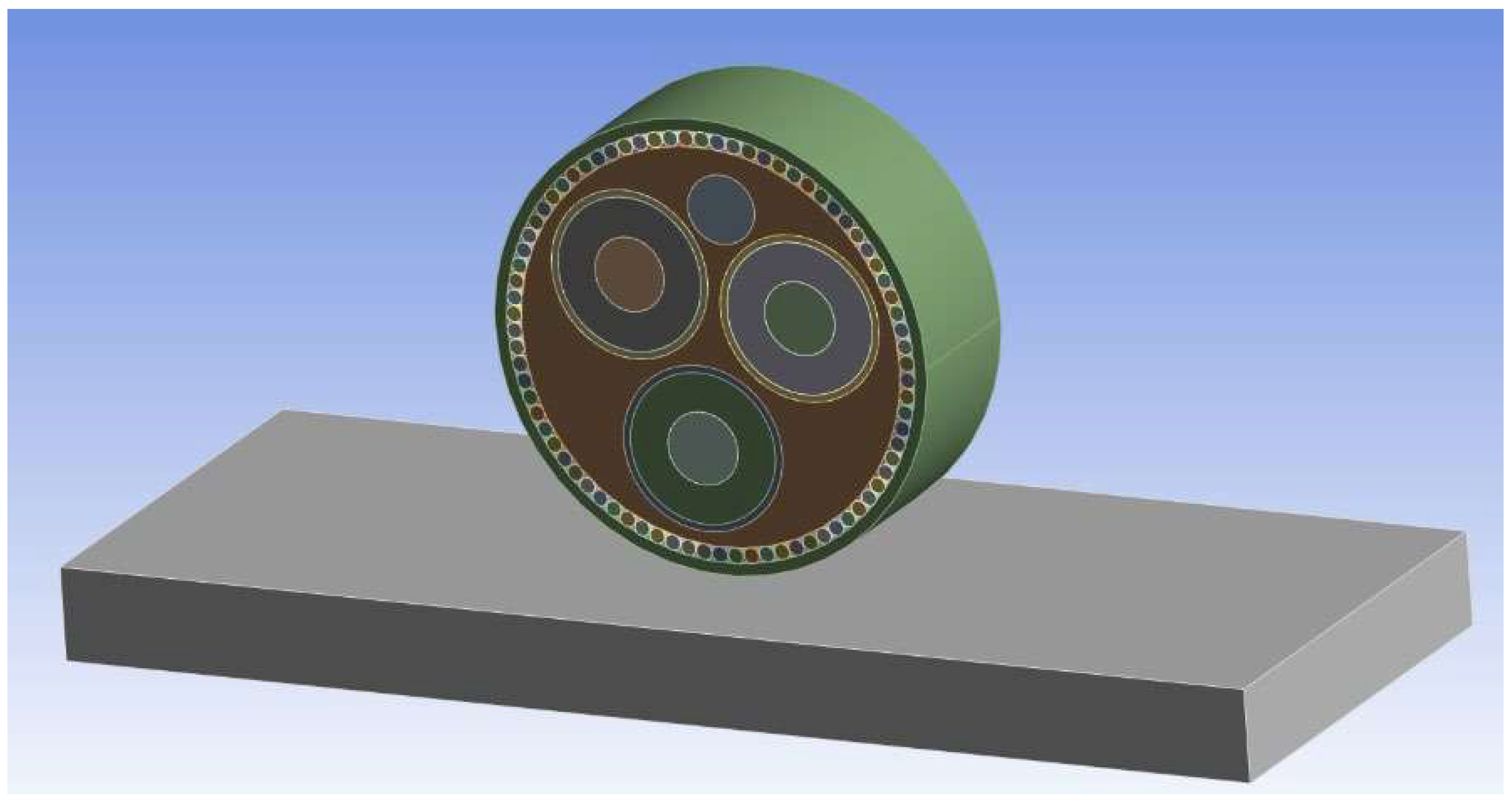
The cable cross-section consists, from the innermost to the outermost layer, of the copper conductor, insulation layer, lead sheath, filling layer, optical fiber, steel wire layer, and outer sheath. The main structural and material parameters are listed in

Table 6. Structural and material parameters of the cable.

Cable Component	Thickness (mm)	Outer Diameter (mm)	Density (kg/m3)	Young’s Modulus (Pa)	Poisson’s Ratio
Copper	-	23.5	8900	1.17 × 1011	0.36
Insulation layer	12.6	48.7	930	8.82 × 108	0.46
Lead sheath	2.3	53.3	11,340	9.78 × 109	0.42
Optical fiber	-	22.5	2203	7.31 × 1010	0.27
Filling layer	-	127.6	950	3.04 × 108	0.46
Steel wire	-	5.0	7800	1.97 × 1011	0.29
Outer sheath	4	145.6	1000	1.55 × 108	0.46

, and the corresponding finite element model is shown in Figure 20. A truncated cable model with a length of 0.1 m is selected for the wear analysis. The contact between the cable and the seabed is modeled using a surface-to-surface contact formulation, in which the outer surface of the cable is defined as the master surface and the seabed surface is defined as the slave surface. The friction coefficient between the contact surfaces is set to 0.15. In the Archard wear model, the dimensionless wear coefficient is taken as K = 1 × 10⁻⁷, and the wear surface hardness of the outer sheath is set to H = 80.

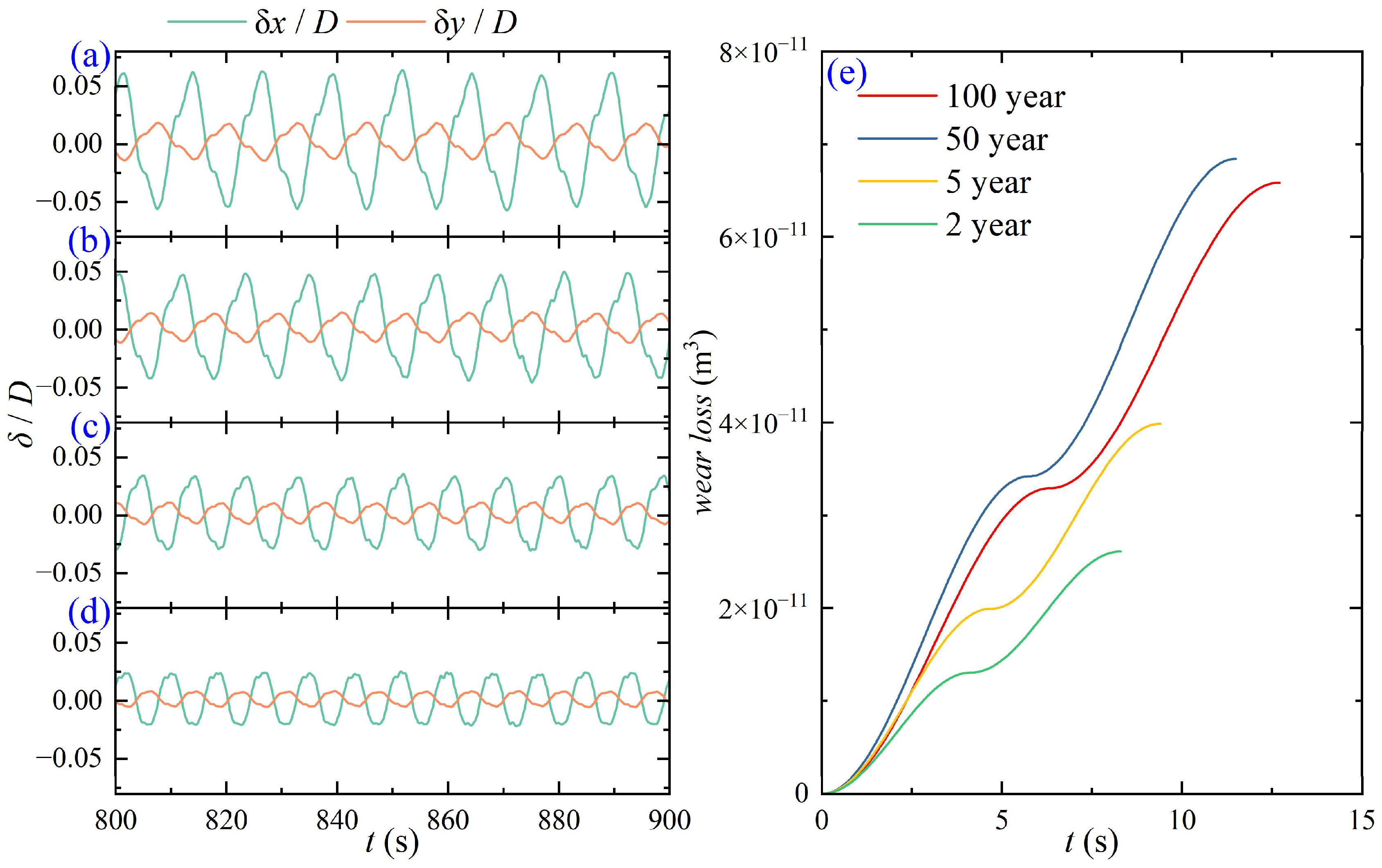
Figure 21 shows the displacement response at the cable touchdown point (TDP) and the evolution of per-cycle wear volume under wave conditions with different return periods. As shown in Figure 21a–d, the displacement amplitudes in both the x- and y-directions at the TDP generally decrease under shorter return periods, with the x-direction displacement as the dominant component. Correspondingly, the wear volume in Figure 21e accumulates gradually with time. The per-cycle wear volumes under the 50-year and 100-year return-period conditions are significantly larger than those under the 5-year and 2-year conditions, indicating that stronger wave action enhances the relative sliding and contact wear between the cable and the seabed. Notably, the per-cycle wear volume does not increase strictly monotonically with the return period. The wear volume under the 50-year return-period condition is slightly higher than that under the 100-year condition.

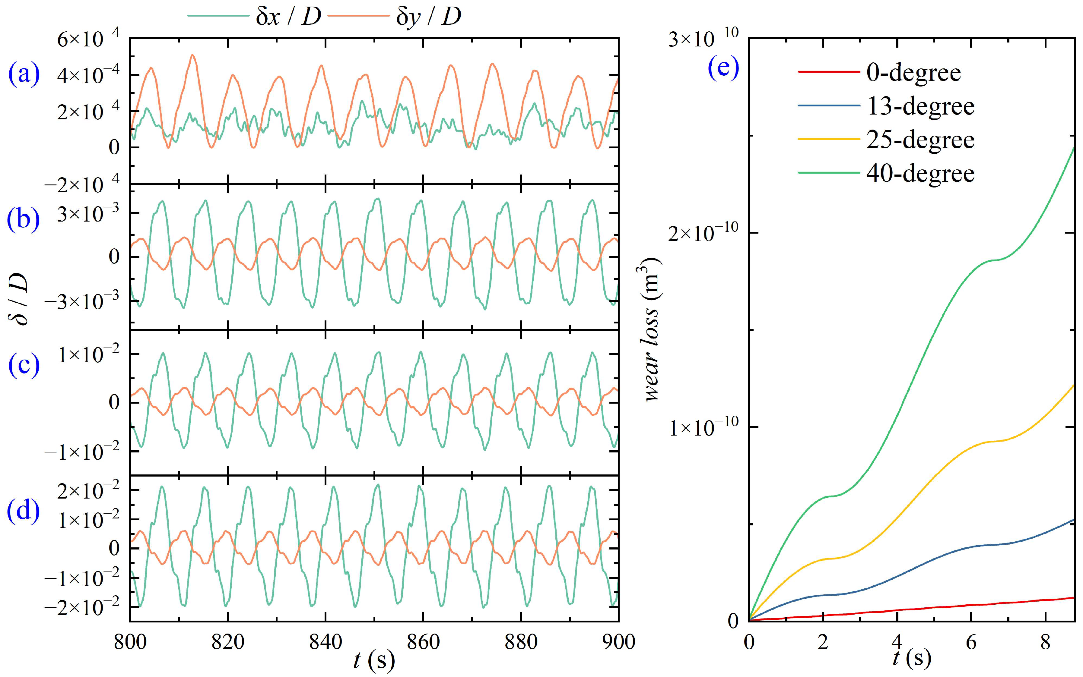
In addition to the wave return period, the wave–current incident angle also influences the wear damage. At the 5-year low-water-level condition, the effect of the wave–current incident angle on cable wear damage is further analyzed, which is shown in Figure 22. When the wave–current angle increases from 0° to 40°, the displacement amplitude at the TDP increases significantly. Correspondingly, the growth rate of wear volume in Figure 22e increases noticeably, and the largest per-cycle wear volume occurs under the 40° condition. This result indicates that oblique wave–current action enhances the reciprocating sliding of the cable in the TDZ, thereby aggravating surface wear of the outer sheath. In contrast, under the 0° condition, the displacement amplitude at the TDP is relatively small, and the wear accumulation is also the weakest. This suggests that the relative sliding between the cable and the seabed is limited under collinear wave–current action.

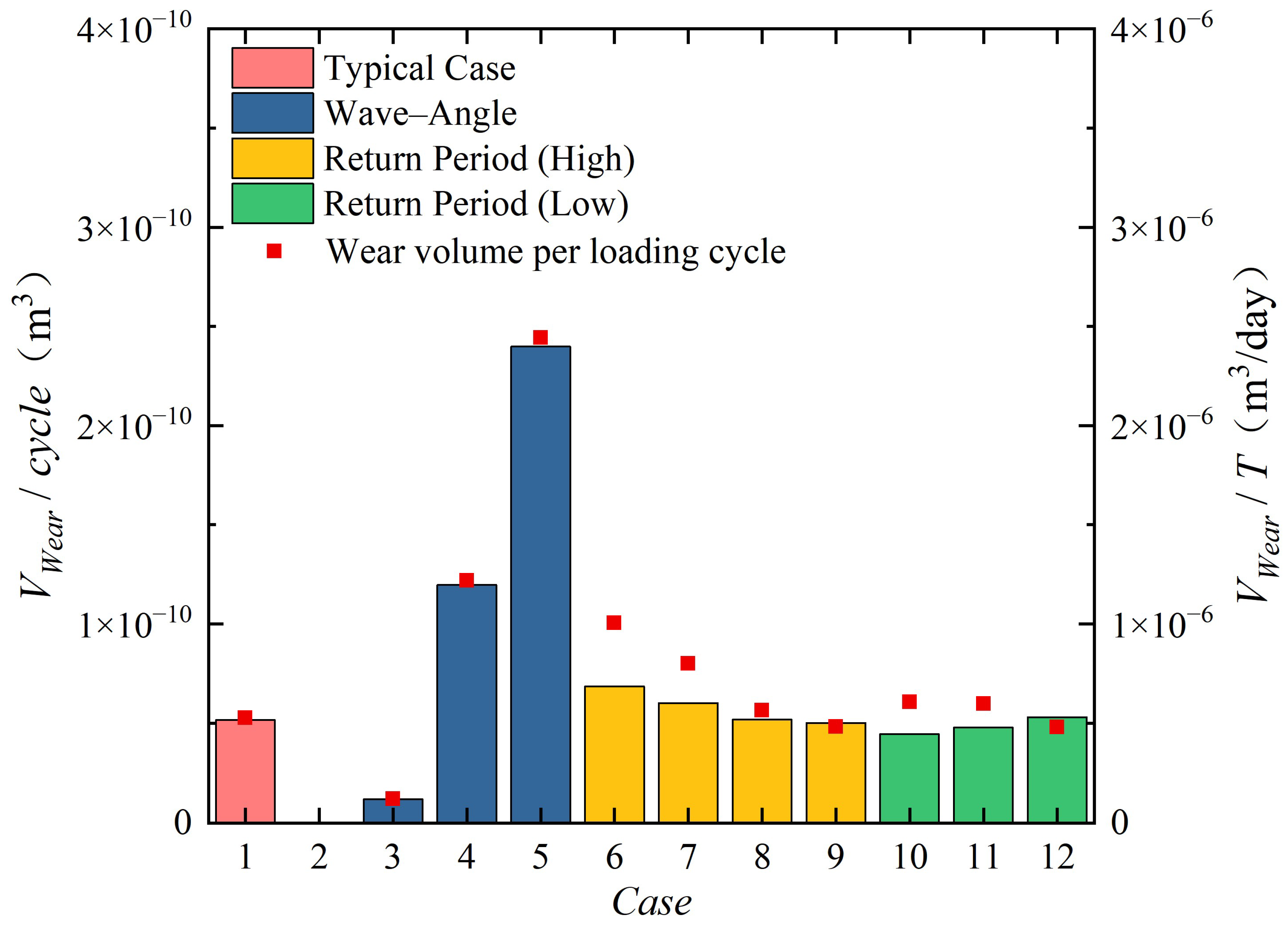
Figure 23 summarizes the per-cycle wear volume of the outer surface under all considered conditions. Compared with the return-period and water-level cases, the wave–current incident angle shows the most pronounced influence on wear damage. In particular, larger-angle cases produce substantially higher wear loss, indicating that the wear response is more sensitive to changes in the direction of wave–current action than to wave intensity alone. Overall, severe outer-sheath wear is closely associated with pronounced reciprocating sliding at the TDP, highlighting the critical role of local relative motion in cable wear.

7. Discussion

The results demonstrate that the combined wave–current conditions significantly affect the dynamic response and damage characteristics of the cable, particularly near the touchdown zone. Variations in wave conditions, water levels, and wave–current angles alter the cable–seabed interaction and consequently influence the distributions of stress, fatigue damage, and wear. These findings highlight the importance of considering environmental variability and nonlinear cable–seabed interaction when assessing the structural integrity of in-service cables.

Several limitations of the present study should be acknowledged. The seabed profile was assumed to remain unchanged throughout the analysis, and possible seabed evolution due to scour, sediment transport, or repeated cable–seabed interaction was not considered. In addition, the contact and wear parameters were prescribed and assumed to remain constant, although they may vary with seabed properties and loading history. The present study focused on the dynamic response, fatigue damage, and wear damage of the cable under combined wave–current action, without explicitly considering vortex-induced vibration (VIV). Under actual current conditions, the suspended span may experience cross-flow vibration, which may alter the local stress cycles and sliding behavior near the TDP. Future work will incorporate evolving seabed conditions and a VIV model to investigate their coupled effects on cable response, seabed contact, fatigue damage, and wear.

8. Conclusions

This study developed a nonlinear dynamic model for a fixed suspended export cable connected to an offshore wind turbine based on the absolute nodal coordinate formulation. The Morison model and cable–seabed interaction model are incorporated to investigate the dynamic response and damage mechanisms of the cable under combined wave–current conditions. In addition, CFD simulations were used to account for the effect of pile-induced flow disturbance on the local flow field. The influences of wave–current angle and metocean conditions on the cable dynamic characteristics were then analyzed. The main conclusions are as follows.

(1) The dynamic response of the cable shows pronounced non-uniformity along its length. Large displacements mainly occur in the suspended span, whereas evident curvature concentration and local stress concentration are observed in the suspended-to-touchdown transition region. The frequency-domain results suggest that a clear frequency-doubling component exists in the total displacement response, while the displacements in each individual direction and tension responses are still mainly governed by the dominant wave frequency. The strength verification shows that the maximum stresses under all analyzed conditions are lower than the allowable stress. This indicates that instantaneous strength failure is not the dominant failure mode for the cable under the considered conditions.

(2) The variation in wave return period mainly affects the response amplitude of the cable, but it does not significantly change the primary response region or the dominant frequency characteristics. Cable tension increases with the wave return period, while its spatial distribution remains nearly unchanged. The curvature distributions under different return periods show only minor differences, demonstrating that the local bending response is mainly controlled by the configuration of the transition region and the seabed boundary condition, rather than by wave intensity alone.

(3) Compared with the change in wave intensity, the wave–current angle has a more significant influence on the cable dynamic response. Increasing the wave–current angle leads to larger displacement amplitudes in the suspended span, higher overall tension levels, and greater curvature in the transition region. Meanwhile, the horizontal displacement trajectories under different angles develop along nearly the same principal direction. This suggests that the incident angle mainly changes the response amplitude along the principal motion direction, but does not significantly alter the direction itself.

(4) The fatigue and wear results show that the damage risk is mainly concentrated in the transition region and near the TDP. The fatigue damage exhibits clear circumferential non-uniformity, and the wave–current angle can affect both the most unfavorable circumferential position and the fatigue distribution. A larger wave–current angle significantly increases the displacement amplitude at the TDP and accelerates the wear accumulation rate. Therefore, under the conditions considered in this study, cyclic bending and contact wear induced by oblique wave–current action are the significant damage modes that require attention.

References

1. Gulski, E.; Jongen, R.; Rakowska, A.; Siodla, K. Offshore wind farms on-site submarine cable testing and diagnosis with damped AC. Energies 2019, 12, 3703. [Google Scholar] [CrossRef] [Scilit]
2. Thies, P.R.; Johanning, L.; Bashir, I.; Tuk, T.; Tuk, M.; Marta, M.; Müller-Schütze, S. Accelerated reliability testing of articulated cable bend restrictor for offshore wind applications. Int. J. Mar. Energy 2016, 16, 65–82. [Google Scholar] [CrossRef] [Scilit]
3. Huera-Huarte, F.J.; Bearman, P.W. Wake structures and vortex-induced vibrations of a long flexible cylinder—Part 1: Dynamic response. J. Fluids Struct. 2009, 25, 969–990. [Google Scholar] [CrossRef] [Scilit]
4. Jain, A.; Modarres-Sadeghi, Y. Vortex-induced vibrations of a flexibly-mounted inclined cylinder. J. Fluids Struct. 2013, 43, 28–40. [Google Scholar] [CrossRef] [Scilit]
5. Xu, W.; Ma, Y.; Ji, C.; Sun, C. Laboratory measurements of vortex-induced vibrations of a yawed flexible cylinder at different yaw angles. Ocean Eng. 2018, 154, 27–42. [Google Scholar] [CrossRef] [Scilit]
6. Dai, M.; Cao, L.; Huang, G.; Zhou, X.; Liu, J.; Chen, Y.F. Dynamic response analysis of mooring cables for floating offshore wind turbines under ocean currents using a perturbation-based finite difference method. Ocean Eng. 2026, 353, 124665. [Google Scholar] [CrossRef] [Scilit]
7. Wang, S.; Wen, H.; Zhang, J.; Zheng, Y.; Zhu, J. Multi-mode response of a flexible catenary cable under oscillating shear flows. Mar. Struct. 2026, 108, 104038. [Google Scholar] [CrossRef] [Scilit]
8. Guo, X.; Luo, Q.; Stoesser, T.; Hajaali, A.; Liu, X. Evolution of high-density submarine turbidity current and its interaction with a pair of parallel suspended pipes. Phys. Fluids 2023, 35, 086608. [Google Scholar] [CrossRef] [Scilit]
9. Nasution, F.P.; Sævik, S.; Berge, S. Experimental and finite element analysis of fatigue strength for 300 mm2 copper power conductor. Mar. Struct. 2014, 39, 225–254. [Google Scholar] [CrossRef] [Scilit]
10. Nasution, F.P.; Sævik, S.; Gjøsteen, J.K.Ø.; Berge, S. Experimental and finite element analysis of fatigue performance of copper power conductors. Int. J. Fatigue 2013, 47, 244–258. [Google Scholar] [CrossRef] [Scilit]
11. Beier, D.; Janocha, M.J.; Ye, N.; Ong, M.C. Fatigue assessment of suspended inter-array power cables for floating offshore wind turbines. Eng. Struct. 2024, 308, 118007. [Google Scholar] [CrossRef] [Scilit]
12. Wang, Y.; Wang, Z.; Li, H.; Huang, X.; Guo, Z. Fretting wear and fatigue life for dynamic power cable conductors under different slip conditions. Mar. Struct. 2025, 103, 103847. [Google Scholar] [CrossRef] [Scilit]
13. Poon, C.; Mhurchadha, S.U.; Barrett, R.A.; Leen, S.B. Three-dimensional representative modelling for fretting wear and fatigue of submarine power cable conductors. Int. J. Fatigue 2024, 184, 108302. [Google Scholar] [CrossRef] [Scilit]
14. Poon, C.; O’Halloran, S.M.; Connolly, A.; Barrett, R.A.; Leen, S.B. Fretting wear and fatigue in submarine power cable conductors for floating offshore wind energy. Tribol. Int. 2023, 186, 108598. [Google Scholar] [CrossRef] [Scilit]
15. Shabana, A.A. Definition of the slopes and the finite element absolute nodal coordinate formulation. Multibody Syst. Dyn. 1997, 1, 339–348. [Google Scholar] [CrossRef] [Scilit]
16. Liu, D.; Li, S.; Ai, S.; Sun, L.; Soares, C.G. Fatigue analysis of steel catenary risers under coupled cross-flow and in-line vortex-induced vibrations with oblique incoming flow. Mar. Struct. 2024, 95, 103578. [Google Scholar] [CrossRef] [Scilit]
17. Zhang, C.; Kang, Z.; Ma, G.; Xu, X. Mechanical modeling of deepwater flexible structures with large deformation based on absolute nodal coordinate formulation. J. Mar. Sci. Technol. 2019, 24, 1241–1255. [Google Scholar] [CrossRef] [Scilit]
18. Zhang, C.; Lu, L.; Cao, Q.; Cheng, L.; Tang, G. Nonlinear motion regimes and phase dynamics of a free standing hybrid riser system subjected to ocean current and vessel motion. Ocean Eng. 2022, 252, 111197. [Google Scholar] [CrossRef] [Scilit]
19. Nielsen, J.D.; Madsen, S.B.; Hyldahl, P.; Balling, O. Dynamic analysis of offshore oil pipe installation using the absolute nodal coordinate formulation. In Proceedings of the ASME International Mechanical Engineering Congress and Exposition, Proceedings (IMECE), San Diego, CA, USA, 1 January 2013; p. ASME. [Google Scholar]
20. Kang, Z.; Li, S.; Zhang, C.; Qu, Y.; Ma, G. Distributions of nonlinear dynamics, stress and fatigue damage along a steel catenary riser in current affected by top-end surge. Ocean Eng. 2023, 285, 115398. [Google Scholar] [CrossRef] [Scilit]
21. Li, S.; Zhang, C.; Kang, Z.; Ai, S. Effects of vertical and lateral riser-soil interactions on vortex-induced vibration of a steel catenary riser. Ocean Eng. 2024, 306, 118075. [Google Scholar] [CrossRef] [Scilit]
22. Randolph, M.; Quiggin, P. Non-linear hysteretic seabed model for catenary pipeline contact. In Proceedings of the International Conference on Ocean, Offshore and Arctic Engineering, Honolulu, HI, USA, 31 May–5 June 2009; ASME: New York, NY, USA, 2009; Volume 3, pp. 145–154. [Google Scholar]
23. Shabana, A.A. Computer implementation of the absolute nodal coordinate formulation for flexible multibody dynamics. Nonlinear Dyn. 1998, 16, 293–306. [Google Scholar] [CrossRef] [Scilit]
24. Miner, M.A. Cumulative Damage in Fatigue. J. Appl. Mech. 2021, 12, A159–A164. [Google Scholar] [CrossRef] [Scilit]
25. Archard, J.F. Contact and Rubbing of Flat Surfaces. J. Appl. Phys. 1953, 24, 981–988. [Google Scholar] [CrossRef] [Scilit]
26. Yu, Y.; Xu, S.; Yu, J.; Xu, W.; Xu, L.; Xu, L. Dynamic analysis of steel catenary riser on the nonlinear seabed using vector form intrinsic finite element method. Ocean Eng. 2021, 241, 109982. [Google Scholar] [CrossRef] [Scilit]
27. Lehmann, M. Esoteric pull and esoteric push: Two simple in-place streaming schemes for the lattice boltzmann method on GPUs. Computation 2022, 10, 92. [Google Scholar] [CrossRef] [Scilit]
Figure 1. Three-dimensional reduced beam element model.
Jmse 14 01565 g001
Figure 2. Schematic diagram of cable system for verification.
Jmse 14 01565 g002
Figure 3. Comparison of (a) configuration; (b) effective tension; and (c) bending moment.
Jmse 14 01565 g003
Figure 4. Schematic diagram of terrain around the wind turbine.
Jmse 14 01565 g004
Figure 5. Time histories of flow velocities of cable section on the suspended and TDZ: (a) x-, (b) y-, and (c) z-direction velocities.
Jmse 14 01565 g005
Figure 6. Computational framework for the dynamic-response, fatigue-damage, and wear-damage analyses of the cable.
Jmse 14 01565 g006
Figure 7. Spatial distribution, time histories, and spectra of the displacement response of the cable under the typical case: (a) spatial distribution; (bd) time histories; and (eg) corresponding spectra.
Jmse 14 01565 g007
Figure 8. Total displacement response at t = 800~900 s under the typical case: (a) spatio-temporal distribution; (b) FFT spectra.
Jmse 14 01565 g008
Figure 9. Statistical characteristics of (a) curvature and (b) tension along the cable under the typical case.
Jmse 14 01565 g009
Figure 10. FFT spectra of the displacement response of the cable under different return periods: (a) 100 years; (b) 50 years; (c) 5 years; (d) 2 years.
Jmse 14 01565 g010
Figure 11. Dynamic responses and corresponding spectra of the cable: (a) x-direction displacement; (b) displacement spectra; (c) tension; and (d) tension spectra.
Jmse 14 01565 g011
Figure 12. Statistical response along the cable arc under various return periods: (a) tension; (b) curvature.
Jmse 14 01565 g012
Figure 13. Total displacement distributions under different wave–current incident angles: (a) 0°; (b) 13°; (c) 25°; and (d) 40°. The arrows indicate the propagation direction of the high-amplitude displacement bands along the cable.
Jmse 14 01565 g013
Figure 14. FFT spectra of total cable displacement under different wave–current incident angles: (a) 0°; (b) 13°; (c) 25°; and (d) 40°.
Jmse 14 01565 g014
Figure 15. Displacement statistics and horizontal trajectories under different wave–current incident angles: (a) statistical distributions; (b) trajectories at the maximum-displacement location.
Jmse 14 01565 g015
Figure 16. Statistical response along the cable arc under various incident angles: (a) tension; (b) curvature.
Jmse 14 01565 g016
Figure 17. Stress distributions of the cable: (a) axial and bending stresses along the cable; (b) combined stress at different circumferential positions.
Jmse 14 01565 g017
Figure 18. Fatigue damage distributions along the cable under various wave return periods and water levels: (a) 100-year return period at high water level; (b) 100-year return period at low water level; (c) 50-year return period at high water level; (d) 50-year return period at low water level; (e) 5-year return period at high water level; (f) 5-year return period at low water level; (g) 2-year return period at high water level; and (h) 2-year return period at low water level.
Jmse 14 01565 g018
Figure 19. Fatigue damage distributions along the cable under different incident angles: (a) 0-degree, (b) 13-degree, (c) 25-degree, and (d) 40-degree incident angles, and (e) pure current condition.
Jmse 14 01565 g019
Figure 20. Three-dimensional cable wear model.
Jmse 14 01565 g020
Figure 21. Touchdown-point displacement at t = 800~900 s and per-cycle wear evolution under different wave return periods: (a) 100-year; (b) 50-year; (c) 5-year; (d) 2-year; and (e) wear volume evolution.
Jmse 14 01565 g021
Figure 22. Touchdown-point displacement histories and per-cycle wear evolution under different wave–current incident angles: (a) 0°; (b) 13°; (c) 25°; (d) 40°; and (e) wear volume evolution.
Jmse 14 01565 g022
Figure 23. Wear volume per loading cycle and daily average wear volume under different conditions. The bars represent the wear volume accumulated over one characteristic loading cycle, and the red squares represent the corresponding daily average wear volume.
Jmse 14 01565 g023