AMF-MUSIC for Underwater Acoustic DOA Estimation Under Strong Interference with Forward-Spatial-Smoothing Extension for Coherent Sources

Abstract

This study evaluates adaptive spatial matrix filtering (AMF) combined with MUSIC for underwater acoustic direction-of-arrival estimation under strong out-of-sector interference and extends the method to coherent sources by incorporating forward spatial smoothing (FSS) into the AMF design. Simulations compared AMF-MUSIC with conventional MUSIC and continuous matrix filter (CMF)-MUSIC. For a 20-sensor array with targets at −2° and 1°, an interferer at 50°, an SNR of −5 dB, and an INR of 20 dB, both AMF-MUSIC and CMF-MUSIC resolved the targets under a common −25 dB stopband bound, but AMF-MUSIC produced a smoother out-of-sector background. Tightening the CMF bound to −40 dB reduced background peaks but degraded target resolution. In coherent-source simulations using a 25-sensor array, AMF-FSS-MUSIC resolved the targets for all tested subarray lengths when the angular separation was at least 4.5°, achieving resolution probabilities of at least 95%. A 900–1100 Hz broadband simulation maintained an approximately −15 dB stopband response and a passband-response error below −12 dB. For the SWellEx-96 narrowband data, AMF-MUSIC reduced the DOA-estimation RMSE from 11.16° to 5.18° and increased the mean spatial-spectrum SIR from −0.41 dB to 13.18 dB, while the broadband results qualitatively demonstrated interference suppression. These results indicate a favorable configuration-dependent suppression–fidelity tradeoff, while robustness to other coherent-source conditions and broader measured-data validation require further investigation.

1. Introduction

Spatial matrix filtering [1,2] is an array signal processing technique that has been developed in recent years. It constructs a filtering matrix [3] and applies it to the received array data to estimate the direction of arrival (DOA) of targets in the region of interest while suppressing interference and noise from regions outside the region of interest. In addition, spatial matrix filtering can be combined with subsequent array signal processing algorithms to improve DOA estimation accuracy and DOA resolution, and it has been widely used in underwater acoustic signal processing [4,5].

Conventional spatial matrix filters have been designed using convex optimization [6], semi-infinite programming [7], minimum-mean-square-error criteria [8], rank-constrained formulations [9], and second-order cone programming [10]. Subsequent studies developed continuous-filter criteria [3] and applied spatial matrix filtering to broadband ship-noise separation [11] and strong-interference cancellation [12]. Because these filters are designed independently of the observed data, their suppression performance is determined primarily by the prescribed passband and stopband constraints.

Data-dependent spatial methods instead use received-data statistics to form nulls near dominant interferers [13,14]. In underwater acoustics, adaptive beamforming and projection-based methods have improved weak-source detection under complex interference [15]. However, these approaches typically produce scalar outputs or detection-oriented projections. An adaptive spatial matrix filter retains a multichannel output and explicitly constrains passband distortion and stopband attenuation, allowing subsequent processing by high-resolution DOA estimators.

Hassanien et al. [16] proposed a dimension-reduced adaptive spatial matrix filter based on convex optimization. This method can effectively attenuate interference and is more robust to interference sources outside the passband sector. However, its filtering performance is limited by the reduced dimensionality. Feng et al. [17] later proposed an adaptive matrix filter design method that does not reduce the dimensionality of the data matrix. In [18], the adaptive spatial matrix filter was applied to matched-field source localization in the presence of strong interference. In [19], a method based on sparse spectral fitting and zero-point matrix filters was proposed for accurately localizing dense wideband signals in strong-interference environments. In [20], a dimension-reduced adaptive antenna design method based on spatial filters was proposed, in which a set of finite impulse response filters is used to construct a lower-rank transformation matrix that converts received data from the element space to the beam space. In [21], the AMF stopband was designed by considering the angular width of the interference spatial spectrum generated under a far-field model. Under near-field source interference, this method increased the output signal-to-interference ratio of the far-field target by 4 dB compared with the conventional method.

Recent studies have addressed related DOA-estimation limitations using several complementary approaches. Hamid et al. [22] developed a robust sparse-reconstruction method for underwater sensor arrays under faulty sensors, low SNR, limited snapshots, and unknown source number. Lin et al. [23] combined projection-based interference blocking with Toeplitz reconstruction for coherent-source DOA estimation under strong interference and non-uniform noise. For covariance-rank restoration, Qi et al. [24] employed Toeplitz matrix reconstruction and a Khatri–Rao subspace to increase the effective degrees of freedom for coherent-source estimation. Zhagypar et al. [25] incorporated spatial smoothing into time-frequency root-MUSIC for coherent and non-stationary sources. Recent broadband approaches have also considered direct time-domain convolutional sparse coding [26] and frequency-domain covariance reconstruction for coherent multi-frequency interference [27]. These studies improve robustness, coherence handling, or broadband processing, but they do not directly consider the use of a forward-spatially-smoothed covariance matrix within the optimization of a full-dimensional data-dependent spatial matrix filter.

Despite these developments, two issues remain insufficiently addressed. Existing full-dimensional AMF studies do not consider covariance-rank restoration for coherent-source DOA estimation, whereas conventional FSS-MUSIC uses the smoothed covariance matrix primarily for subspace estimation rather than for data-dependent spatial-filter design. In addition, measured-data evaluation of full-dimensional AMF-MUSIC using actual nonuniform underwater-array geometry remains limited.

The contributions of this study are summarized as follows:

• The full-dimensional AMF formulation in [17] is adopted as a spatial prefilter and combined with MUSIC for underwater acoustic DOA estimation under strong out-of-sector interference. The AMF formulation and MUSIC are reused components and are not individually claimed as new developments.
• For coherent sources, the FSS covariance matrix is incorporated into the data-dependent AMF optimization before MUSIC processing. This constitutes the principal algorithmic extension relative to conventional FSS-MUSIC, in which spatial smoothing is used primarily for subspace estimation.
• A frequency-dependent subband implementation is considered for broadband processing, and the AMF-MUSIC processing chain is evaluated using simulations and SWellEx-96 data with measured nonuniform array geometry. The SWellEx-96 results provide quantitative narrowband and qualitative broadband measured-data evidence, while the coherent-source extension is supported only by preliminary simulations under the investigated configuration.

Table 1. Comparison of the proposed method with representative existing approaches.

Method	Filter Design	Data Dependence	Coherent Sources	Broadband Processing	Computational Cost	Validation
Full-dimensional AMF [17]	Constrained adaptive matrix filter	Yes	Not considered	Not reported	High; convex optimization	Simulations
Conventional FSS-MUSIC [28,29]	No adaptive matrix filter	Covariance-dependent	Yes	Not considered in the cited formulation	Moderate; FSS and eigen decomposition	Established simulations and applications
Wideband MFN-SpSF [19]	Adaptive nulling matrix filter with sparse spectrum fitting	Yes	Not specifically considered	Yes	High; filter and sparse optimization	Simulations and experiments
Present method	Constrained AMF combined with MUSIC	Yes	Yes; FSS covariance is also used in AMF design	Yes; subband AMFs and spectrum combination	High; SOCP, FSS, and MUSIC	AMF-MUSIC: simulations and SWellEx-96 data; AMF-FSS-MUSIC: coherent-source simulations only

summarizes the differences between the present method and the most relevant existing approaches.

The remainder of this paper is organized as follows. Section 2 introduces the signal model and the basic principle of spatial matrix filtering. Section 3 presents the adopted AMF formulation, its extension to coherent-source processing using forward spatial smoothing, the broadband implementation, the SOCP solution, and the computational-complexity analysis. Section 4 describes the numerical simulations and evaluates the proposed processing methods under the investigated non-coherent and coherent-source conditions. Section 5 presents a quantitative narrowband evaluation and a qualitative broadband evaluation of AMF-MUSIC using the SWellEx-96 experimental data. Section 6 discusses the performance mechanisms, applicable conditions, limitations, relationship to previous methods, and computational feasibility. Section 7 concludes the paper.

2. Basic Principles of Spatial Matrix Filtering

Consider an array with $M$ elements. When $D$ uncorrelated far-field narrowband signals impinge on the array, their DOAs are denoted by

$${\mathsf{\Theta }}_D=\left\{{\theta }_1,{\theta }_2,\dots ,{\theta }_D\right\}.$$

The received array data can be expressed as

$$\mathbf{x}\left(t\right)=\mathbf{A}\left({\mathsf{\Theta }}_D\right)\mathbf{s}\left(t\right)+\mathbf{n}\left(t\right),$$

(1)

where $\mathbf{x}\left(t\right)\in {\mathbb{C}}^{M\times 1}$ is the received array-data vector at time $t$, $\mathbf{s}\left(t\right)\in {\mathbb{C}}^{D\times 1}$ is the source-signal vector, and $\mathbf{n}\left(t\right)\in {\mathbb{C}}^{M\times 1}$ is the additive-noise vector. The array manifold matrix is defined as

$$\mathbf{A}\left({\mathsf{\Theta }}_D\right)=\left[\mathbf{a}\left({\theta }_1\right),\mathbf{a}\left({\theta }_2\right),\dots ,\mathbf{a}\left({\theta }_D\right)\right]\in {\mathbb{C}}^{M\times D}$$

where $\mathbf{a}\left({\theta }_d\right)$ denotes the steering vector corresponding to the $d$-th source DOA ${\theta }_d$.

For the uniform linear array used in the numerical simulations, $\theta =0°$ denotes the array broadside direction, and the first sensor is used as the phase reference. The steering vector is explicitly defined as

$$\mathbf{a}\left(\theta ,f\right)={\left[1,\hspace{0.17em}{e}^{-\mathrm{j}k\left(f\right)d\sin \theta },\hspace{0.17em}{e}^{-\mathrm{j}k\left(f\right)2d\sin \theta },\hspace{0.17em}\dots ,\hspace{0.17em}{e}^{-\mathrm{j}k\left(f\right)\left(M-1\right)d\sin \theta }\right]}^T,$$

where

$$k\left(f\right)={\displaystyle \frac{2\pi f}{c}}.$$

Here, $d$ is the interelement spacing, $c$ is the propagation speed, and $k\left(f\right)$ is the wavenumber. The superscript ${\left(·\right)}^T$ denotes the transpose. Positive angles follow the phase convention $-k\left(f\right)d\sin \theta$. The model assumes narrowband far-field plane-wave propagation. For broadband processing, the same model is applied separately at the center frequency of each narrowband subband.

The spatial matrix filter $\mathbf{G}$ is designed as an $M\times M$ matrix, and the filtered output is given by

$$\mathit{y}\left(t\right)={\mathit{G}}^H\mathit{x}\left(t\right)=\mathit{C}\left({\mathsf{\Theta }}_D\right)\mathit{s}\left(t\right)+{\mathit{n}}_c\left(t\right),$$

(2)

where $\mathbf{G}\in {\mathbb{C}}^{M\times M}$ is the spatial matrix filter; the superscript ${\left(·\right)}^H$ denotes the conjugate transpose; and $\mathbf{y}\left(t\right)\in {\mathbb{C}}^{M\times 1}$ is the filtered multichannel output, where

$$\mathbf{C}\left({\mathsf{\Theta }}_D\right)={\mathbf{G}}^H\mathbf{A}\left({\mathsf{\Theta }}_D\right),$$

and

$${\mathbf{n}}_c\left(t\right)={\mathbf{G}}^H\mathbf{n}\left(t\right).$$

The designed spatial matrix filter should pass signals from the region of interest and suppress signals from outside the region of interest. Then the filter meets the requirements [3].

$$G^{H}a(\theta )=\left\{\begin{array}{l}a(\theta ),\begin{array}{cc}& \theta \in {\mathsf{\Theta }}_P\end{array}\\ 0,\begin{array}{ccc}& & \theta \in {\mathsf{\Theta }}_S\end{array}\end{array}\right.,$$

(3)

where ${\mathsf{\Theta }}_P$ and ${\mathsf{\Theta }}_S$ denote the prescribed passband and stopband angular sectors, respectively. The symbols ${\theta }_p\in {\mathsf{\Theta }}_P$, $p=1,\dots ,P$, and ${\theta }_s\in {\mathsf{\Theta }}_S$, $s=1,\dots ,S$, denote the sampled passband and stopband directions, respectively; $P$ and $S$ are the corresponding numbers of angular samples. The vector $\mathbf{0}\in {\mathbb{C}}^{M\times 1}$ denotes the all-zero vector.

3. Design of the Adaptive Spatial Matrix Filter

3.1. Design of Adaptive Spatial Matrix Filter

The full-dimensional adaptive spatial matrix filter formulation adopted in this study follows Feng et al. [17] and is summarized here to define the optimization used in the subsequent processing. The formulation itself is not claimed as a new contribution. The AMF is designed to minimize the total output power while satisfying prescribed passband-response and stopband-response constraints.

Because the filtered multichannel output is $\mathbf{y}\left(t\right)={\mathbf{G}}^H\mathbf{x}\left(t\right)$, its total output power is the real non-negative scalar

$$\begin{array}{cc}\hfill J\left(\mathbf{G}\right)& =\mathbb{E}\left\{{\Vert \mathbf{y}\left(t\right)\Vert }_2^2\right\}\hfill \\ & =\mathbb{E}\left\{\mathrm{tr}\left[\mathbf{y}\left(t\right){\mathbf{y}}^H\left(t\right)\right]\right\} ,\hfill \\ & =\mathrm{tr}\left({\mathbf{G}}^H{\mathbf{R}}_x\mathbf{G}\right)\hfill \end{array}$$

(4)

where $\left(\mathbb{E}\cdot \right)$ denotes statistical expectation, $\mathrm{tr}\left(\cdot \right)$ denotes the matrix trace, and

$${\mathbf{R}}_x=\mathbb{E}\left\{\mathbf{x}\left(t\right){\mathbf{x}}^H\left(t\right)\right\}$$

is the covariance matrix of the received array data. Therefore, the AMF design problem is formulated as

$$\begin{array}{cc}\hfill \underset{\mathbf{G}}{\min } & \mathrm{tr}\left({\mathbf{G}}^H{\mathbf{R}}_x\mathbf{G}\right)\hfill \\ \hfill \mathrm{s}.\mathrm{t}.& {\Vert {\mathbf{G}}^H\mathbf{a}\left({\theta }_p\right)-\mathbf{a}\left({\theta }_p\right)\Vert }_2\le \xi , {\theta }_p\in {\mathsf{\Theta }}_P ,\hfill \\ & {\Vert {\mathbf{G}}^H\mathbf{a}\left({\theta }_s\right)\Vert }_2\le \delta , {\theta }_s\in {\mathsf{\Theta }}_S\hfill \end{array}$$

(5)

where ${\Vert \cdot \Vert }_2$ denotes the Euclidean norm, $\xi \ge 0$ is the maximum allowable passband-response error, and $\delta \ge 0$ is the prescribed upper bound on the stopband-response amplitude. The optimization variable is $\mathbf{G}\in {\mathbb{C}}^{M\times M}$, and $\mathbf{a}\left(\theta \right)\in {\mathbb{C}}^{M\times 1}$ is the steering vector at direction $\theta$.

To obtain the vectorized form, define

$$\mathbf{g}=\mathrm{vec}\left({\mathbf{G}}^H\right)\in {\mathbb{C}}^{M^2\times 1},$$

and factorize the covariance matrix as

$${\mathbf{R}}_x={\mathbf{Q}}^H\mathbf{Q},$$

where $\mathbf{Q}\in {\mathbb{C}}^{M\times M}$. A Cholesky factor can be used when ${\mathbf{R}}_x$ is positive definite; otherwise, any valid matrix square-root factor satisfying the above equality may be used. By applying the standard vectorization identity

$$\mathrm{vec}\left(\mathbf{A}\mathbf{B}\mathbf{C}\right)=\left({\mathbf{C}}^T\otimes \mathbf{A}\right)\mathrm{vec}\left(\mathbf{B}\right),$$

the objective in Equation (5) can be written as

$$\begin{array}{cc}\hfill \underset{\mathbf{g}}{\min } & {\Vert \left({\mathbf{Q}}^{\ast }\otimes {\mathbf{I}}_M\right)\mathbf{g}\Vert }_2^2\hfill \\ \hfill s.t.& {\Vert \left[{\mathbf{a}}^T\left({\theta }_p\right)\otimes {\mathbf{I}}_M\right]\mathbf{g}-\mathbf{a}\left({\theta }_p\right)\Vert }_2\le \xi .\hfill \\ & {\Vert \left[{\mathbf{a}}^T\left({\theta }_s\right)\otimes {\mathbf{I}}_M\right]\mathbf{g}\Vert }_2\le \delta \hfill \end{array}$$

(6)

Here, ${\mathbf{I}}_M\in {\mathbb{C}}^{M\times M}$ is the $M\times M$ identity matrix, and $\mathbf{g}\in {\mathbb{C}}^{M^2\times 1}$. The matrices satisfy ${\mathbf{Q}}^{\ast }\otimes {\mathbf{I}}_M\in {\mathbb{C}}^{M^2\times M^2}$ and ${\mathbf{a}}^T\left(\theta \right)\otimes {\mathbf{I}}_M\in {\mathbb{C}}^{M\times M^2}$. The objective contains an $M^2$-dimensional complex vector, whereas each passband or stopband constraint contains an $M$-dimensional complex vector. The squared Euclidean norm in the objective is a real non-negative scalar. Minimizing the squared norm is equivalent to minimizing the norm because the square function is strictly increasing for non-negative arguments. In the SOCP implementation described in Section 3.3, a real scalar epigraph variable is introduced to express the objective in standard second-order cone form.

For broadband AMF processing, the analysis band is divided into narrow frequency subbands. A frequency-dependent covariance matrix, steering vector, and AMF are constructed for each subband using the same angular passband and stopband definitions. The spatial spectra obtained from the individual subbands are then combined for broadband DOA estimation.

3.2. Adaptive Spatial Matrix Filtering for Coherent Signals

Because coherent signals commonly occur in real marine environments, DOA estimation for coherent sources requires additional decorrelation processing. The spatial smoothing algorithm [29] is incorporated into the adaptive spatial-matrix-filtering-based interference suppression method to suppress coherent interference and estimate the DOAs of coherent sources.

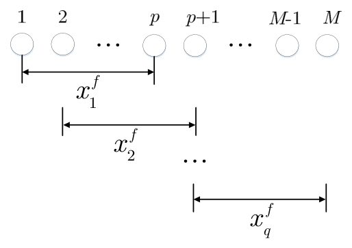
For forward spatial smoothing (FSS), the $M$-element uniform linear array is divided into $q$ maximally overlapping subarrays, each containing $p$ elements, where

$$q=M-p+1.$$

The index $l=1,\dots ,q$ denotes the subarray number. The FSS procedure is illustrated in Figure 1.

The received signal of each subarray is

$$\left\{\begin{array}{l}{\mathit{x}}_1^f={[x_1,x_2,\dots ,x_p]}^T\\ {\mathit{x}}_2^f={[x_2,x_3,\dots ,x_{p+1}]}^T\\ \begin{array}{cccc}& & & ⋮\end{array}\\ {\mathit{x}}_q^f={[x_q,x_{q+1},\dots ,x_M]}^T\end{array}\right.$$

(7)

where ${\mathit{x}}_l^f\left(t\right)\in {\mathbb{C}}^{p\times 1}$ is the received-data vector of the $l$-th forward subarray, and the superscript $f$ denotes forward spatial smoothing.

The output vector ${\mathit{x}}_l^f$ of the l-th subarray can be expressed as

$${\mathbf{x}}_l^f={\mathbf{A}}_p\left(\theta \right){\mathbf{F}}^{(l-1)}\mathbf{s}\left(t\right)+{\mathbf{n}}_l\left(t\right),$$

(8)

where ${\mathbf{A}}_p\left(\theta \right)$ is the subarray manifold matrix; ${\mathit{F}}^{ l-1}$ represents the phase shift associated with the $l$-th overlapping subarray; $\mathbf{s}\left(t\right)$ is the source-signal vector defined after Equation (1); and ${\mathbf{n}}_l\left(t\right)$ is the noise vector of the $l$-th subarray. Assuming the number of sources is $D$, $\mathbf{F}$ can be written as

$$\mathbf{F}=\mathrm{diag}\left[e^{-j{\omega }_1},{\mathrm{e}}^{-j{\omega }_2},\dots ,e^{-j{\omega }_D}\right],$$

(9)

where $\mathrm{diag}\left(\cdot \right)$ denotes a diagonal matrix; $j=\sqrt{-1}$ is the imaginary unit; and ${\omega }_d$ is the interelement spatial phase shift of the $d$-th source. For a half-wavelength uniform linear array, ${\omega }_d$ is determined by the incident direction ${\theta }_d$ according to the adopted steering-vector convention.

Assuming spatially white noise with variance ${\sigma }^2$, the covariance matrix of the $l$-th forward subarray is

$${\mathbf{R}}_l^f={\mathbf{A}}_p{\mathbf{F}}^{l-1}{\mathbf{R}}_s{\left({\mathbf{F}}^{l-1}\right)}^H{\mathbf{A}}_p^H+{\sigma }^2{\mathbf{I}}_p,$$

(10)

where ${\mathbf{R}}_l^f\in {\mathbb{C}}^{p\times p}$ and ${\mathbf{I}}_p$ is the $p\times p$ identity matrix. The forward-spatially-smoothed covariance matrix is then obtained by averaging the covariance matrices of all overlapping subarrays:

$${\mathbf{R}}^f={\mathbf{A}}_p\left[{\displaystyle \frac{1}{q}}{\displaystyle \sum _{l=1}^q}{\mathbf{F}}^{l-1}{\mathbf{R}}_s{\left({\mathbf{F}}^{l-1}\right)}^H\right]{\mathbf{A}}_p^H+{\sigma }^2{\mathbf{I}}_p.$$

(11)

Because every diagonal entry of $\mathbf{F}$ has unit magnitude, $\mathbf{F}$ is unitary. Therefore,

$${\mathbf{F}}^H\mathbf{F}=\mathbf{F}{\mathbf{F}}^H=\mathbf{I},$$

and

$${\left({\mathbf{F}}^{\hspace{0.17em}l-1}\right)}^H={\mathbf{F}}^{-\left(l-1\right)}.$$

Accordingly, Equations (10) and (11) use the explicit Hermitian form to make the covariance construction and conjugate-transpose operation unambiguous.

For $K_{\mathrm{c}}$ mutually coherent sources with distinct directions, forward spatial smoothing can restore the covariance rank when the number of overlapping subarrays satisfies

$$q\ge K_{\mathrm{c}}.$$

Meanwhile, the subarray length should satisfy

$$p>K_{\mathrm{c}},$$

to retain a nonempty noise subspace for MUSIC. Since

$$q=M-p+1,$$

the admissible subarray length is therefore

$$K_{\mathrm{c}}+1\le p\le M-K_{\mathrm{c}}+1.$$

Spatial smoothing reduces the effective aperture from $\left(M-1\right)d$ to $\left(p-1\right)d$. Consequently, the nominal aperture-limited angular-resolution scale is increased approximately by a factor of

$${\displaystyle \frac{M-1}{p-1}}.$$

Thus, a larger $p$ retains better angular resolution, whereas a smaller $p$ provides more overlapping subarrays for covariance-rank restoration.

The smoothed covariance matrix ${\mathbf{R}}^f\in {\mathbb{C}}^{p\times p}$ is substituted for ${\mathbf{R}}_x$ in Equation (5), or equivalently in Equation (6). The full-array dimension $M$ is simultaneously replaced by the subarray dimension $p$, and $\mathbf{a}\left(\theta \right)$ is replaced by the subarray steering vector ${\mathbf{a}}_p\left(\theta \right)$. The resulting coherent-source AMF is therefore

$${\mathbf{G}}_f\in {\mathbb{C}}^{p\times p}.$$

After applying this filter, the covariance matrix and steering vector supplied to MUSIC are, respectively,

$${\mathbf{G}}_f^H{\mathbf{R}}^f{\mathbf{G}}_f,$$

and

$${\mathbf{G}}_f^H{\mathbf{a}}_p\left(\theta \right),$$

MUSIC is then applied using the eigen decomposition of ${\mathbf{R}}_{\mathrm{A}\mathrm{M}\mathrm{F}}^f$ and the corresponding filtered steering vector. Unlike conventional FSS-MUSIC, in which ${\mathbf{R}}^f$ is used directly for subspace estimation, the present processing chain first uses ${\mathbf{R}}^f$ to design the data-dependent AMF and then performs MUSIC using the AMF-filtered covariance matrix.

3.3. Second-Order Cone Programming

To show explicitly how the AMF problem in Equation (6) is implemented, define

$${\mathbf{C}}_0={\mathbf{Q}}^{\ast }\otimes {\mathbf{I}}_M\in {\mathbb{C}}^{M^2\times M^2}, {\mathbf{C}}_{\theta }={\mathbf{a}}^T\left(\theta \right)\otimes {\mathbf{I}}_M\in {\mathbb{C}}^{M\times M^2}.$$

(12)

Because minimizing a non-negative norm and its square gives the same optimizer, Equation (6) is equivalently written in the following CVX-compatible form:

$$\begin{array}{cc}\hfill \underset{\mathbf{g}\in {\mathbb{C}}^{M^2}}{\mathrm{m}\mathrm{i}\mathrm{n}\mathrm{i}\mathrm{m}\mathrm{i}\mathrm{z}\mathrm{e}}& {\Vert {\mathbf{C}}_0\mathbf{g}\Vert }_2\hfill \\ \hfill \mathrm{s}\mathrm{u}\mathrm{b}\mathrm{j}\mathrm{e}\mathrm{c}\mathrm{t} \mathrm{t}\mathrm{o}& {\Vert {\mathbf{C}}_{\theta }\mathbf{g}-\mathbf{a}\left(\theta \right)\Vert }_2\le \xi , \theta \in {\mathsf{\Theta }}_{\mathrm{p}},\hfill \\ & {\Vert {\mathbf{C}}_{\theta }\mathbf{g}\Vert }_2\le \delta , \theta \in {\mathsf{\Theta }}_{\mathrm{s}}.\hfill \end{array}$$

(13)

Here, the objective and the left-hand side of each constraint are scalar Euclidean norms. CVX permits complex optimization variables and complex affine expressions to be entered directly in the form of Equation (13).

For completeness, the equivalent real-valued cone representation can be obtained by defining, for any complex vector $\mathbf{z}\in {\mathbb{C}}^r$,

$$\mathcal{R}\left(\mathbf{z}\right)=\left[\begin{array}{c}\mathrm{Re}\left(\mathbf{z}\right)\\ \mathrm{Im}\left(\mathbf{z}\right)\end{array}\right]\in {\mathbb{R}}^{2r}, \mathbf{z}\in {\mathbb{C}}^r.$$

(14)

and, for any complex matrix $\mathbf{A}\in {\mathbb{C}}^{s\times r}$,

$$\mathcal{E}\left(\mathbf{A}\right)=\left[\begin{array}{cc}\mathrm{Re}\left(\mathbf{A}\right)& -\mathrm{Im}\left(\mathbf{A}\right)\\ \mathrm{Im}\left(\mathbf{A}\right)& \mathrm{Re}\left(\mathbf{A}\right)\end{array}\right]\in {\mathbb{R}}^{2s\times 2r}, \mathbf{A}\in {\mathbb{C}}^{s\times r}.$$

(15)

These definitions satisfy

$$\mathcal{R}\left(\mathbf{A}\mathbf{z}\right)=\mathcal{E}\left(\mathbf{A}\right)\mathcal{R}\left(\mathbf{z}\right), {\Vert \mathbf{A}\mathbf{z}\Vert }_2={\Vert \mathcal{E}\left(\mathbf{A}\right)\mathcal{R}\left(\mathbf{z}\right)\Vert }_2.$$

(16)

Accordingly, define

$${\tilde{\mathbf{C}}}_0=\mathcal{E}\left({\mathbf{C}}_0\right), {\tilde{\mathbf{C}}}_{\theta }=\mathcal{E}\left({\mathbf{C}}_{\theta }\right).$$

(17)

Introducing the real scalar epigraph variable (t), the real-valued SOCP solved internally by CVX is

$$\begin{array}{cc}\hfill \underset{\tilde{\mathbf{g}}\in {\mathbb{R}}^{2M^2},\hspace{0.17em}t\in \mathbb{R}}{\mathrm{m}\mathrm{i}\mathrm{n}\mathrm{i}\mathrm{m}\mathrm{i}\mathrm{z}\mathrm{e}}& t\hfill \\ \hfill \mathrm{s}\mathrm{u}\mathrm{b}\mathrm{j}\mathrm{e}\mathrm{c}\mathrm{t} \mathrm{t}\mathrm{o}& {\Vert {\tilde{\mathbf{C}}}_0\tilde{\mathbf{g}}\Vert }_2\le t,\hfill \\ & {\Vert {\tilde{\mathbf{C}}}_{\theta }\tilde{\mathbf{g}}-\tilde{\mathbf{a}}\left(\theta \right)\Vert }_2\le \xi , \theta \in {\mathsf{\Theta }}_{\mathrm{p}},\hfill \\ & {\Vert {\tilde{\mathbf{C}}}_{\theta }\tilde{\mathbf{g}}\Vert }_2\le \delta , \theta \in {\mathsf{\Theta }}_{\mathrm{s}},\hfill \\ & t\ge 0.\hfill \end{array}$$

(18)

Thus, the AMF objective and every passband or stopband constraint are expressed as scalar second-order cone inequalities. In the implementation, Equation (13) is entered directly using the complex-variable support of CVX, which internally performs the real embedding represented by Equations (14)–(18). The complete AMF-MUSIC processing sequence for one data segment is summarized in Algorithm 1.

Algorithm 1. AMF-MUSIC processing for one data segment

Input: Array-data matrix $\mathbf{X}$, passband grid, stopband grid, passband tolerance $\xi$, stopband bound $\delta$, and MUSIC search grid.

Estimate the sample covariance matrix from the current data segment. Construct the passband and stopband steering-vector matrices using an angular interval of (1°). Form the AMF optimization problem using the estimated covariance matrix. Solve the optimization problem with CVX and reshape the solution vector into the matrix filter. Apply the resulting matrix filter to the current array-data segment. Estimate the covariance matrix of the filtered data. Calculate the MUSIC spatial spectrum on a (0.1°) angular grid. Identify the DOA estimates from the spatial-spectrum peaks.

Output: Filtered MUSIC spatial spectrum and estimated DOAs.

3.4. Computational Complexity and Real-Time Feasibility

Let $M$ be the number of sensors, $L$ the number of snapshots, $K_p$ and $K_s$ the numbers of sampled passband and stopband directions, respectively, $G$ the MUSIC search-grid size, and $B$ the number of frequency subbands. Estimating the sample covariance matrix requires $O\left(M^{2}L\right)$ operations, while its dense factorization requires $O\left(M^3\right)$ operations. The $M\times M$ complex adaptive matrix filter contains $M^2$ complex unknowns, corresponding to approximately $n=2M^2$ real decision variables after real-valued embedding. For a generic dense primal–dual interior-point implementation, factorization of the Newton system has an $O\left(n^3\right)$ leading-order dependence per iteration. Therefore, a conservative unstructured estimate for the optimization stage is $O\left(N_{\mathrm{i}\mathrm{t}}{M}^6\right)$, where $N_{\mathrm{i}\mathrm{t}}$ is the number of interior-point iterations. The actual computational cost also increases with $K_p+K_s$ and depends strongly on the cone structure and solver implementation.

For MUSIC processing, the covariance-matrix eigen decomposition requires $O\left(M^3\right)$ operations, and evaluation over the angular search grid requires $O\left(G{M}^2\right)$ operations. For forward spatial smoothing, let $P$ denote the subarray length and $J=M-P+1$ the number of maximally overlapping subarrays. The covariance-formation cost is approximately $O\left(J{P}^{2}L\right)$, followed by an $O\left(P^3\right)$ eigendecomposition and an $O\left(G{P}^2\right)$ spectral search. In broadband processing, the covariance estimation, AMF design, and spectrum evaluation are repeated for $B$ independently processed frequency subbands; therefore, their overall costs increase approximately linearly with $B$. However, the subband calculations can be parallelized.

The current implementation employs CVX with a general-purpose interior-point solver. Although CVX provides a convenient and reliable framework for formulating the AMF optimization problem, it does not by itself guarantee real-time implementation. Because no hardware-specific runtime benchmark is available for the present implementation, the results reported in this study support offline or blockwise processing but do not establish hard real-time operation. A real-time implementation would require the measured optimization latency to remain below the filter-update interval. Its computational burden could be reduced through parallel subband processing, a lower AMF update rate, reduced passband and stopband angular grids, warm starts where supported, and a customized solver that exploits the structure of the AMF optimization problem.

4. Simulations and Performance Analysis

Unless otherwise specified, the simulations consider far-field plane waves received by a uniform horizontal linear array in a homogeneous acoustic medium. The sound speed is 1500 m/s, and the interelement spacing is 0.75 m. The common and experiment-specific settings are summarized in

Table 2. Summary of the principal simulation settings.

Case	Array and Filter Configuration	Source Model and DOAs	SNR and INR	Evaluation Settings
Common settings	Homogeneous medium; sound speed: 1500 m/s; interelement spacing: 0.75 m; sampling frequency: 5 kHz; duration: 1 s; 5000 samples	Far-field plane waves	Post-filtering powers referenced to the average noise power per sensor	AMF and CMF constraint-grid interval: 1°; MUSIC grid: 0.1°; passband tolerance: 1.65; no diagonal loading
Simulation 1: narrowband response	20-element UHLA; aperture: 14.25 m; AMF stopband setting: −25 dB; CMF setting: −40 dB	Two non-coherent targets at −2° and 1°; interferer at 50°; center frequency: 1 kHz; bandwidth: 20 Hz	Target SNR: 0 dB; INR: 40 dB	Single-configuration filter-response comparison
Simulation 1: broadband response	20-element UHLA; 20 Hz frequency subbands	Target at 5°; interferer at −40°; source band: 900–1100 Hz	SNR: −10 dB; INR: 20 dB	Prescribed AMF stopband attenuation: −15 dB
Simulation 2: representative DOA comparison	20-element UHLA; MUSIC; AMF stopband setting: −25 dB; CMF stopband setting: −25 dB controlled comparison and −40 dB sensitivity case	Two non-coherent targets at −2° and 1°; interferer at 50°	SNR: −5 dB; INR: 20 dB	Same array data; representative single realization
Simulation 3: SNR variation	20-element UHLA; AMF-MUSIC and CMF-MUSIC; AMF stopband setting: −25 dB; CMF stopband setting: −40 dB	Two non-coherent targets at −2° and 1°; interferer at 50°	SNR: −15 to 15 dB in 2.5 dB increments; INR: 20 dB	200 Monte Carlo trials at each SNR
Simulation 4: INR variation	20-element UHLA; AMF stopband setting: −25 dB; CMF stopband setting: −30 dB	Two non-coherent targets at −2° and 1°; interferer at 50°	SNR: −10 dB; INR: −5 to 25 dB in 2.5 dB increments	200 Monte Carlo trials at each INR
Simulation 5a: coherent-source baseline and SNR variation	25-element UHLA; aperture: 18 m; five maximally overlapping subarrays of 21 sensors; normalized AMF stopband bound: −25 dB	Two coherent targets at −2° and 3°; coherent interferer at 50°; frequency: 1 kHz	Representative target SNR: −5 dB; SNR sweep: −20 to 15 dB in 2.5 dB increments; INR: 20 dB	AMF-MUSIC and AMF-FSS-MUSIC comparison; 200 Monte Carlo trials at each SNR in the sweep
Simulation 5b: coherent-source angular-separation and subarray-length variation	25-element UHLA; aperture: 18 m; maximally overlapping subarrays of 20, 21, 22, and 23 sensors; normalized AMF stopband bound: −25 dB	Target 1 fixed at −2°; Target 2 varied from 0° to 4° in 0.5° increments, corresponding to separations of 2–6°; coherent interferer at 50°; frequency: 1 kHz	Target SNR: −5 dB; INR: 20 dB	200 paired Monte Carlo trials; resolution probability and conditional RMSE

.

In the non-coherent simulations, the target, interference, and sensor-noise sequences are generated independently using randn and passed through their prescribed bandpass filters. Let $s_d\left[n\right]$, $i_r\left[n\right]$, and $n_m\left[n\right]$ denote the resulting unscaled sequences. Their finite-sample powers are calculated after filtering as

$$\begin{gathered} {\widehat{P}}_{s,d}^{\left(0\right)}={\displaystyle \frac{1}{N}}{\displaystyle \sum _{n=0}^{N-1}}{\left|{\tilde{s}}_d\left[n\right]\right|}^2, \\ {\widehat{P}}_{i,r}^{\left(0\right)}={\displaystyle \frac{1}{N}}{\displaystyle \sum _{n=0}^{N-1}}{\left|{\tilde{i}}_r\left[n\right]\right|}^2, \\ {\widehat{P}}_n={\displaystyle \frac{1}{MN}}{\displaystyle \sum _{m=1}^M}{\displaystyle \sum _{n=0}^{N-1}}{\left|{\tilde{n}}_m\left[n\right]\right|}^2. \\ {s}_d\left[n\right]=\sqrt{{\displaystyle \frac{{\widehat{P}}_n{10}^{{\mathrm{S}\mathrm{N}\mathrm{R}}_d/10}}{{\widehat{P}}_{s,d}^{\left(0\right)}}}}\hspace{0.17em}{\tilde{s}}_d\left[n\right], \\ {i}_r\left[n\right]=\sqrt{{\displaystyle \frac{{\widehat{P}}_n{10}^{{\mathrm{I}\mathrm{N}\mathrm{R}}_r/10}}{{\widehat{P}}_{i,r}^{\left(0\right)}}}}\hspace{0.17em}{\tilde{i}}_r\left[n\right]. \\ {\mathrm{S}\mathrm{N}\mathrm{R}}_d=10{\log }_{10}\left({\displaystyle \frac{{\widehat{P}}_{s,d}}{{\widehat{P}}_n}}\right),{\mathrm{I}\mathrm{N}\mathrm{R}}_r=10{\log }_{10}\left({\displaystyle \frac{{\widehat{P}}_{i,r}}{{\widehat{P}}_n}}\right). \end{gathered}$$

The SNR is defined separately for each target and the INR separately for each interference source. Both are input power ratios referenced to the average post-filtering noise power per sensor before spatial filtering and therefore exclude array gain.

For each data segment, the sample covariance matrix is calculated from the array-data matrix as follows.

$${\widehat{\mathbf{R}}}_x={\displaystyle \frac{1}{N}}\mathbf{X}{\mathbf{X}}^H,\mathbf{X}\in {\mathbb{C}}^{M\times N}.$$

For the representative single-realization and measured-data analyses, the same array-data matrix is used for covariance estimation, AMF design, and filtered MUSIC processing, and the AMF is redesigned for each data segment. For the Monte Carlo evaluations, one AMF is designed at each tested parameter setting using an independently generated training dataset and then applied to the corresponding evaluation trials; the compared methods use identical evaluation data wherever applicable. Unless otherwise specified, no diagonal loading is applied, and the AMF optimization is solved using CVX 2.2 with SDPT3 4.0 and the default precision setting. The remaining simulation parameters are listed in Table 2.

For each Monte Carlo trial, the two largest local maxima above −40 dB were selected over the complete −90° to 90° MUSIC search range and paired with the ground-truth DOAs in ascending angular order. The mean estimate, RMSE, and MAE were calculated without applying an angular-error gate. A trial was considered successfully resolved when two distinct peaks were detected and both paired DOA errors did not exceed 1°; all other trials were counted as resolution failures.

$$P_{\mathrm{r}\mathrm{e}\mathrm{s}}={\displaystyle \frac{1}{N_{\mathrm{M}\mathrm{C}}}}{\displaystyle \sum _{r=1}^{N_{\mathrm{M}\mathrm{C}}}}\mathbb{I}\left(\left|{\hat{\theta }}_{1,r}-{\theta }_1\right|\le 1°\hspace{0.33em}\wedge \hspace{0.33em}\left|{\hat{\theta }}_{2,r}-{\theta }_2\right|\le 1°\right),$$

where $\mathbb{I}\left(\cdot \right)$ is the indicator function. This probability complements the estimation-error measures by explicitly counting trials in which both targets are simultaneously resolved.

Let $N_{\mathrm{M}\mathrm{C}}$ be the number of Monte Carlo trials, ${\theta }_i$ the ground-truth DOA of Target $i$, and ${\widehat{\theta }}_{i,r}$ its paired estimate in the $r$-th trial. The mean estimate, RMSE, and MAE are defined below. The reported RMSE and MAE are the arithmetic means of the corresponding target-wise values.

$$\begin{gathered} {\overline{\widehat{\theta }}}_i={\displaystyle \frac{1}{N_{\mathrm{M}\mathrm{C}}}}{\displaystyle \sum _{r=1}^{N_{\mathrm{M}\mathrm{C}}}}{\widehat{\theta }}_i^{\left(r\right)}, i=\mathrm{1,2}, \\ {\mathrm{RMSE}}_i=\sqrt{{\displaystyle \frac{1}{N_{\mathrm{M}\mathrm{C}}}}{\displaystyle \sum _{r=1}^{N_{\mathrm{M}\mathrm{C}}}}{\left({\widehat{\theta }}_i^{\left(r\right)}-{\theta }_i\right)}^2}, i=\mathrm{1,2}, \\ {\mathrm{MAE}}_i={\displaystyle \frac{1}{N_{\mathrm{M}\mathrm{C}}}}{\displaystyle \sum _{r=1}^{N_{\mathrm{M}\mathrm{C}}}}\left|{\widehat{\theta }}_i^{\left(r\right)}-{\theta }_i\right|, i=\mathrm{1,2}. \end{gathered}$$

4.1. Adaptive Spatial Matrix Filtering

Simulation Experiment 1: Spatial Matrix Filter Responses.

The narrowband responses of the AMF and CMF are first evaluated using the Simulation 1 configuration summarized in Table 2. The angular passband and stopband sectors are defined as follows:

$$\begin{gathered} {\mathsf{\Theta }}_{\mathrm{p}}=\left[-15°,15°\right], \\ {\mathsf{\Theta }}_{\mathrm{s}}=\left[-90°,-20°\right]\cup \left[20°,90°\right]. \end{gathered}$$

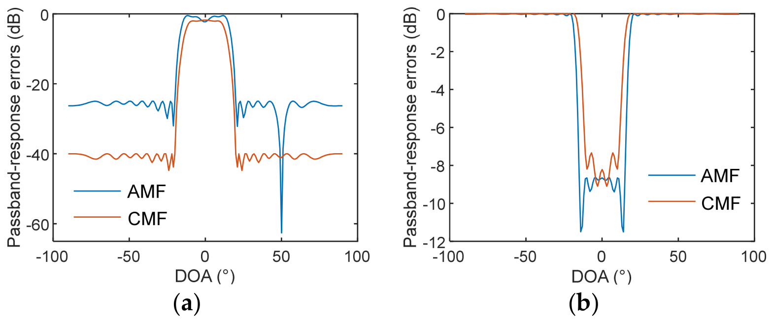
The prescribed AMF stopband attenuation is −25 dB, whereas the CMF is designed using a −40 dB stopband setting under the stopband-constrained passband minimum-mean-square-error criterion. Figure 2 compares the amplitude responses and passband-response errors of the two filters.

As shown in Figure 2, the data-dependent AMF forms a deep null near the interference DOA of 50° while maintaining the prescribed passband response. Because the AMF and CMF use different stopband settings in this retained simulation, Figure 2 should be interpreted as a comparison of the two adopted filter configurations rather than as a fully controlled assessment of adaptivity alone.

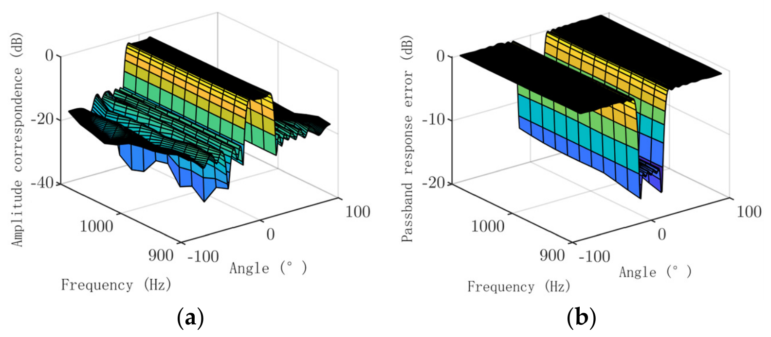
The broadband response of the AMF is subsequently evaluated using the corresponding configuration summarized in Table 2. A frequency-dependent steering vector and AMF are constructed for each 20 Hz subband. Figure 3 presents the broadband amplitude response and passband-response error.

As shown in Figure 3, the stopband attenuation remains approximately −15 dB, while the passband-response error remains below −12 dB. A deep null is formed near the −40° interference direction across the considered frequency subbands. These results demonstrate the filter response obtained for the investigated broadband configuration.

Simulation Experiment 2: Representative DOA Comparison and Constraint-Sensitivity Analysis.

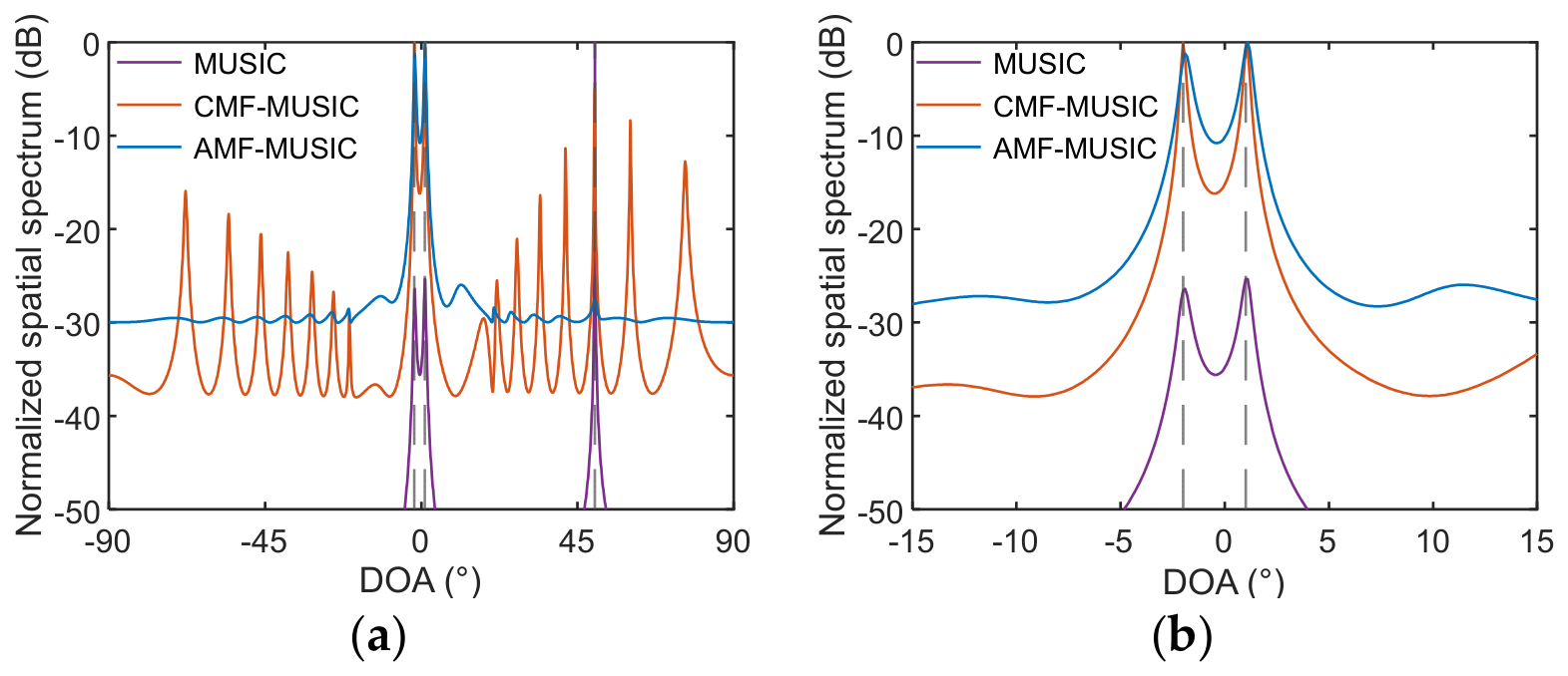
A controlled comparison was first conducted using conventional MUSIC, CMF-MUSIC, and AMF-MUSIC. All three methods processed the same simulated array data. CMF and AMF used the same −25 dB stopband bound, with two targets at −2° and 1° at an SNR of −5 dB and an interferer at 50° at an INR of 20 dB.

As shown in Figure 4, the conventional MUSIC spectrum is dominated by the out-of-sector interferer at 50°, although target-related peaks remain visible in the enlarged target-sector view. Under the common −25 dB stopband bound, both CMF-MUSIC and AMF-MUSIC resolve the two targets. CMF-MUSIC produces several relatively high out-of-sector local maxima, whereas AMF-MUSIC exhibits a comparatively smooth background. Because each spectrum is normalized by its own maximum, Figure 4 provides a qualitative comparison of spectral shapes rather than a quantitative measure of interference attenuation.

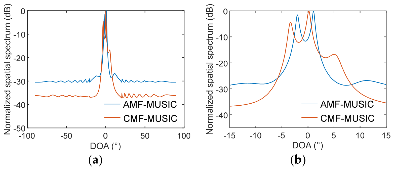
To examine whether the out-of-sector local maxima of CMF-MUSIC could be reduced by a tighter constraint, the CMF stopband bound was subsequently changed from −25 to −40 dB, while the AMF bound remained at its nominal value of −25 dB.

As shown in Figure 5, tightening the CMF bound substantially reduces its out-of-sector local maxima but increases passband distortion and degrades the resolution of the two closely spaced targets. For the investigated CMF design, these results demonstrate a tradeoff between out-of-sector background suppression and target-sector fidelity: the −25 dB bound preserves the two target peaks but permits higher background maxima, whereas the −40 dB bound suppresses these maxima at the expense of target resolution.

For the subsequent Monte Carlo experiments, the CMF bound was fixed at −40 dB to retain stronger out-of-sector background suppression, while the AMF bound was fixed at its feasible nominal value of −25 dB. Therefore, the following results compare the adopted method-specific configurations and should not be interpreted as an equal-constraint assessment of data dependence alone.

Simulation Experiment 3: DOA Estimation Performance under Different SNR Conditions.

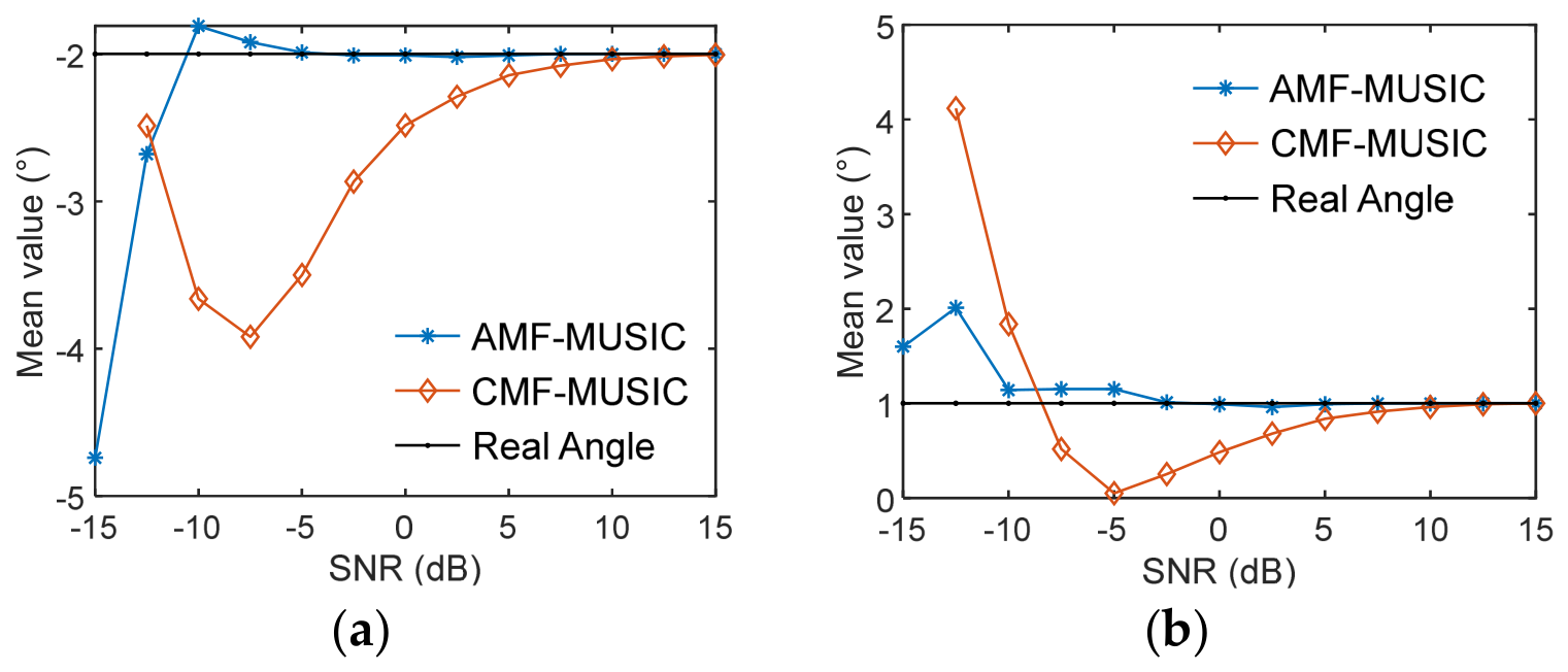
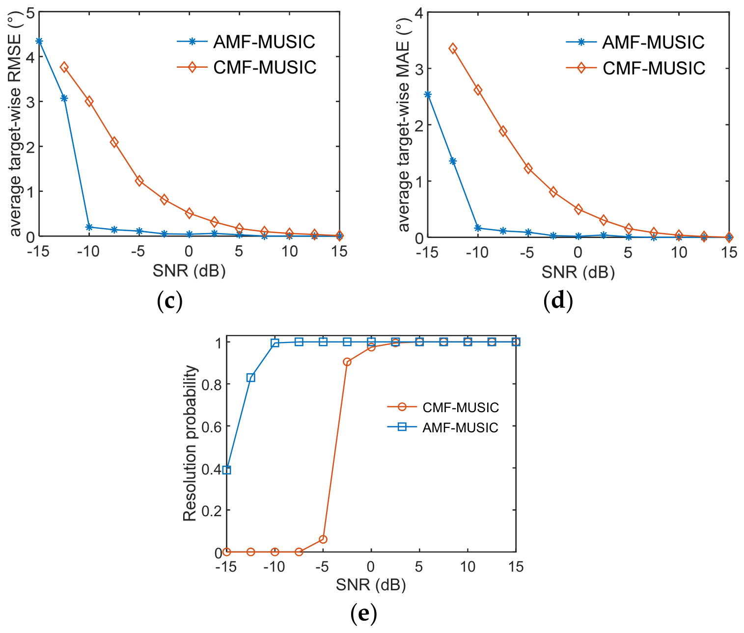
For the SNR-dependent Monte Carlo evaluation, CMF-MUSIC and AMF-MUSIC processed the same simulated array data in each trial. The target SNR was varied from −15 to 15 dB in 2.5 dB increments, while the INR was fixed at 20 dB. The CMF and AMF stopband bounds were −40 dB and −25 dB, respectively. At each SNR, 200 independent Monte Carlo trials were performed. Figure 6 presents the mean estimates, average target-wise RMSE and MAE, and two-target resolution probability.

Figure 6a,b show that the mean estimates approach the two ground-truth DOAs as the SNR increases. Figure 6c,d show corresponding decreases in RMSE and MAE. At low SNRs, the large estimation errors mainly result from the selection of residual or interference-related peaks rather than small deviations of correctly identified target peaks. Under the adopted method-specific constraints, AMF-MUSIC generally produces smaller estimation errors than CMF-MUSIC.

Figure 6e further shows the two-target resolution probability. For AMF-MUSIC, the probability increases from 0.39 at −15 dB to 0.83 at −12.5 dB and 0.995 at −10 dB, reaching 1.0 at −7.5 dB. CMF-MUSIC produces no successful two-target trials from −15 to −7.5 dB, after which its probability increases to 0.905 at −2.5 dB and reaches 1.0 at 5 dB. The probability result confirms that the large low-SNR errors are associated with resolution failures. Because CMF and AMF use stopband bounds of −40 dB and −25 dB, respectively, these results characterize the adopted filter configurations and do not isolate the effect of data dependence alone.

Simulation Experiment 4: DOA Estimation Performance at Different Interference-to-Noise Ratios.

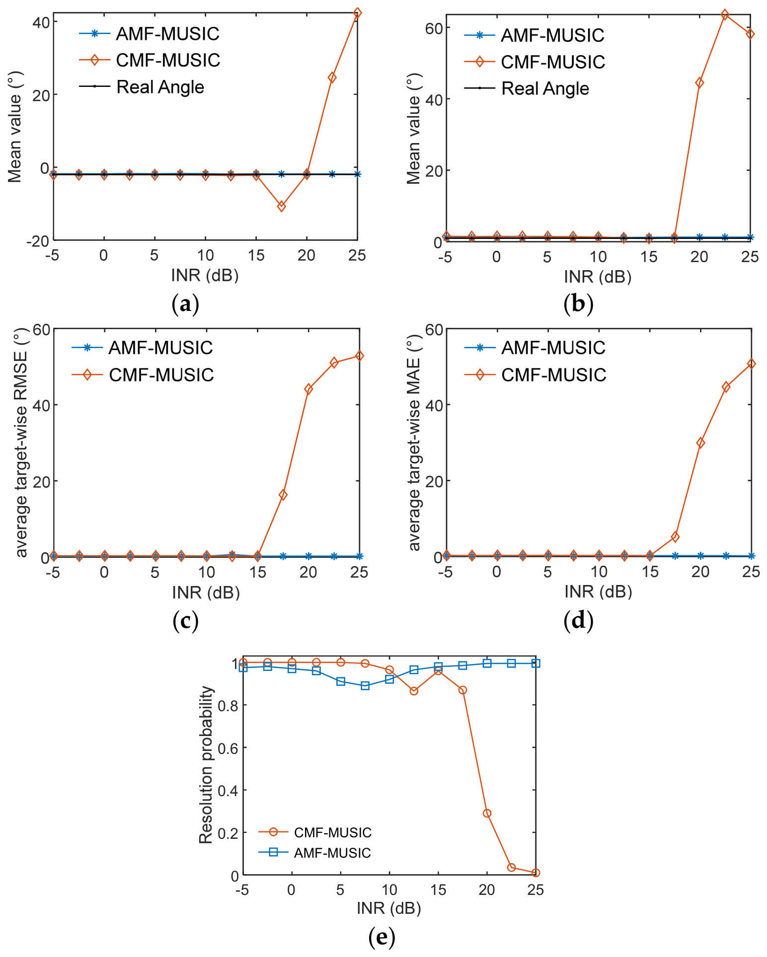
For the INR-dependent Monte Carlo evaluation, the target SNR was fixed at −10 dB, while the INR was varied from −5 to 25 dB in 2.5 dB increments. The CMF and AMF stopband bounds were −30 dB and −25 dB, respectively. At each INR, 200 independent paired trials were conducted, with both methods processing the same simulated array data. Figure 7 presents the mean estimates, average target-wise RMSE and MAE, and two-target resolution probability.

Figure 7a–d show that AMF-MUSIC remains comparatively stable as the INR increases, whereas the CMF-MUSIC estimation errors increase substantially in the high-INR region. The two-target resolution probability in Figure 7e provides a more direct indication of this difference. The AMF-MUSIC probability remains between 0.89 and 0.995 over the complete investigated INR range and reaches 0.995 at INRs of 20–25 dB.

CMF-MUSIC maintains a high resolution probability at low and moderate INRs, but its probability decreases from 0.87 at 17.5 dB to 0.29 at 20 dB, 0.035 at 22.5 dB, and 0.01 at 25 dB. This decrease is consistent with the increasing selection of the strong out-of-sector interference peak. Under the adopted configurations, AMF-MUSIC therefore provides more stable two-target resolution in the high-INR region. However, CMF and AMF use stopband bounds of −30 dB and −25 dB, respectively; thus, the observed difference cannot be attributed exclusively to data dependence.

4.2. Coherent-Source Performance of AMF-FSS-MUSIC

Simulation Experiment 5: Performance Comparison of DOA Estimation.

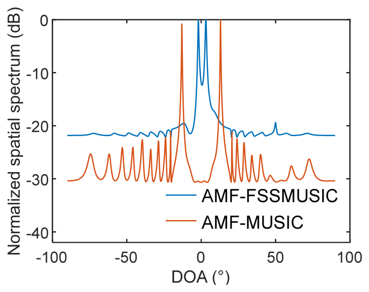
The coherent-source simulation uses the configuration summarized in Table 2. The two target signals and the interference are generated as complex exponential signals at 1 kHz, with initial phases of π/2, π, and 0, respectively. Therefore, the two targets and the interference are mutually coherent.

The 25-element array is divided into five maximally overlapping forward subarrays, each containing 21 sensors. For the three coherent sources considered here, the subarray length and number of overlapping subarrays satisfy the rank-restoration conditions described in Section 3.2 while retaining a nonempty noise subspace for MUSIC. Figure 8 compares the spatial spectra obtained using AMF-MUSIC without spatial smoothing and AMF-FSS-MUSIC.

As shown in Figure 8, AMF-MUSIC without spatial smoothing does not resolve the two coherent targets because of the rank deficiency of the covariance matrix. After forward spatial smoothing, AMF-FSS-MUSIC produces two distinguishable target peaks at −1.9° and 3.1°, corresponding to an absolute DOA estimation error of 0.1° for each target under this representative configuration.

Forward spatial smoothing reduces the effective aperture from 24 interelement spacings for the full array to 20 interelement spacings for each subarray, corresponding to a reduction from 18 to 15 m. Consequently, the nominal aperture-limited angular-resolution scale increases by a factor of 1.2, representing an approximate 20% loss in nominal angular resolution. Nevertheless, the two targets remain resolvable for the angular separation considered in this simulation. This result illustrates the tradeoff between covariance-rank restoration and effective-aperture reduction.

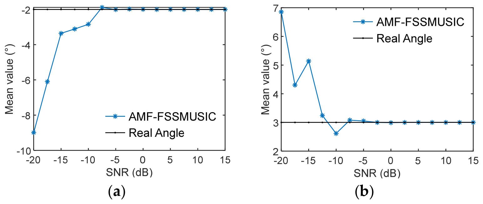
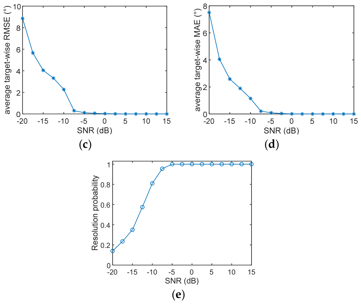
The SNR dependence of AMF-FSS-MUSIC was subsequently evaluated from −20 to 15 dB in 2.5 dB increments, with the INR fixed at 20 dB. Figure 9 reports the mean DOA estimates, average target-wise RMSE and MAE, and two-target resolution probability.

Figure 9a–d show that the mean estimates approach the two ground-truth DOAs and that the RMSE and MAE generally decrease as the SNR increases. At low SNRs, the two strongest selected peaks frequently do not correspond simultaneously to the two targets, resulting in relatively large mean-estimation errors, RMSEs, and MAEs. These error measures therefore include the effect of resolution failures and should be interpreted together with the resolution probability.

As shown in Figure 9e, the two-target resolution probability increases from 0.14 at −20 dB to 0.35 at −15 dB and exceeds 0.5 at −12.5 dB. It further increases to 0.81 at −10 dB and 0.955 at −7.5 dB, reaching 1.0 at −5 dB. These results show that AMF-FSS-MUSIC reliably resolves the two coherent targets under the investigated conditions when the SNR is approximately −7.5 dB or higher, whereas resolution failures become increasingly frequent at lower SNRs.

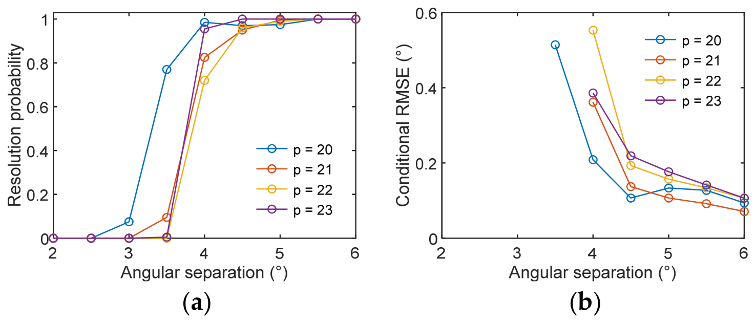
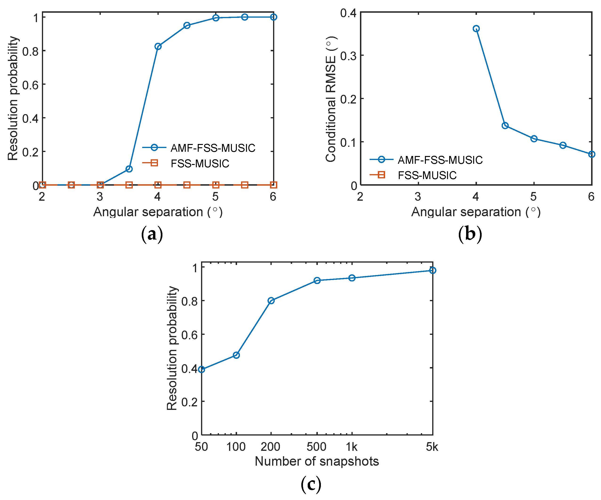
To further evaluate the coherent-source performance, the target angular separation was varied from 2° to 6° in 0.5° increments, with Target 1 fixed at −2°. Subarray lengths of 20, 21, 22, and 23 sensors were considered. The target SNR and INR were fixed at −5 dB and 20 dB, respectively. A trial was regarded as successfully resolved when two distinct target peaks were detected and both absolute DOA errors were within 1°. Figure 10 shows that all tested subarray lengths achieved resolution probabilities of at least 95% when the target separation was 4.5° or greater, while the conditional RMSE generally decreased as the angular separation increased.

To provide a direct baseline comparison, conventional FSS-MUSIC was evaluated using the 21-element subarrays. Both methods processed the same array data in each of the 200 paired Monte Carlo trials and used identical spatial-smoothing, full-angle MUSIC-search, source-number, peak-selection, and resolution-success settings. Conventional FSS-MUSIC applied MUSIC directly to the forward-spatially-smoothed covariance matrix, whereas AMF-FSS-MUSIC applied the adaptive matrix filter before MUSIC processing. The robustness of AMF-FSS-MUSIC to limited snapshots was also evaluated using 50, 100, 200, 500, 1000, and 5000 snapshots. The coherent targets remained at −2° and 3° with an SNR of −5 dB, while the coherent interferer remained at 50° with an INR of 20 dB. The subarray length was fixed at 21 sensors, and 200 Monte Carlo trials were performed for each snapshot number.

As shown in Figure 11a, conventional FSS-MUSIC did not successfully select both targets in any of the investigated configurations because the strong coherent interferer at 50° was consistently included among the two strongest peaks. This result does not imply that target-related peaks were absent; rather, conventional FSS-MUSIC could not simultaneously identify both targets under the adopted full-angle two-peak selection rule. In contrast, the resolution probability of AMF-FSS-MUSIC was 82.5% at a separation of 4°, increased to 95.0% at 4.5°, and reached 100% at separations of 5.5° and 6°. Figure 11b shows that its conditional RMSE decreased from 0.362° at 4° to 0.071° at 6°. No conditional RMSE is reported for conventional FSS-MUSIC because it produced no successful two-target trials. The comparison therefore demonstrates the benefit of adaptive interference suppression for identifying both coherent targets in the presence of the strong out-of-sector interferer.

Figure 11c shows that the two-target resolution probability increased from 0.390 with 50 snapshots to 0.800 with 200 snapshots, 0.920 with 500 snapshots, and 0.980 with 5000 snapshots. Meanwhile, the conditional RMSE calculated from successfully resolved trials decreased from 0.500° to 0.103°. These results show that limited sample support degrades covariance estimation and target resolution, whereas the performance becomes increasingly stable as the number of snapshots increases.

The additional tests broaden the coherent-source validation with respect to target angular separation, subarray length, and snapshot number. However, robustness to coherence level, source number, interference direction, INR, and model mismatch remains to be investigated.

5. Experimental Data Processing

The AMF-based interference suppression algorithm is evaluated using the SWellEx-96 experimental data [30], including a quantitative narrowband analysis and a qualitative broadband analysis.

5.1. Experimental Setup

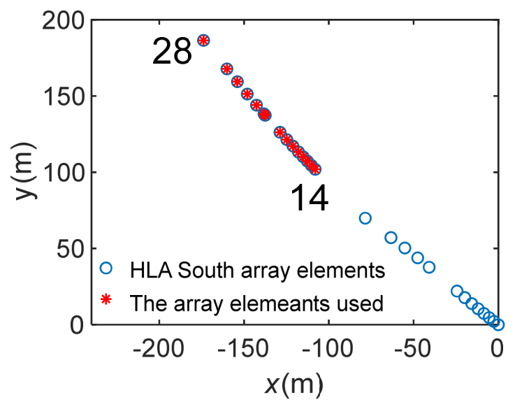
The SWellEx-96 experiment was conducted in May 1996, approximately 12 km off Point Loma, near San Diego, California. The experiment comprised a vertical line array (VLA), a tilted line array (TLA), HLA North, and HLA South. Event S59 contains a source tow and a loud interferer. This study uses the public SWellEx-96 Event S59 HLA South file J1341145.hla.south.sio.gz, which was read using sioread.m. The distributed file contains 28 processed channels after the archive-identified faulty elements have been removed. Channels 14–28 of the processed file were used, corresponding to physical array elements 17–30 and 32. Their measured horizontal coordinates, rather than an idealized uniform spacing, are shown in Figure 12 relative to the array origin; the positive x-axis points east and the positive y-axis points north.

It should be noted that the array configuration in the SWellEx-96 experiment differs from the ideal uniform horizontal linear array assumed in the numerical simulations. For experimental data processing, the actual three-dimensional coordinates of the selected hydrophone elements are used to construct the array manifold matrix. Specifically, the steering vector corresponding to a scanning direction is calculated according to the actual element positions:

$$\mathbf{a}\left(\theta \right)={\left[e^{-jk{\mathbf{r}}_1^T\mathbf{u}\left(\theta \right)},e^{-jk{\mathbf{r}}_2^T\mathbf{u}\left(\theta \right)},\dots ,e^{-jk{\mathbf{r}}_M^T\mathbf{u}\left(\theta \right)}\right]}^T,$$

where ${\mathbf{r}}_m={\left[x_m,y_m,z_m\right]}^T$ denotes the measured position vector of the $m$-th hydrophone, $k$ is the acoustic wavenumber, and $\mathbf{u}\left(\theta \right)$ represents the unit propagation vector corresponding to the scanning direction. Therefore, the spatial matrix filter and MUSIC estimator both account for the actual non-uniform geometry of the HLA South array.

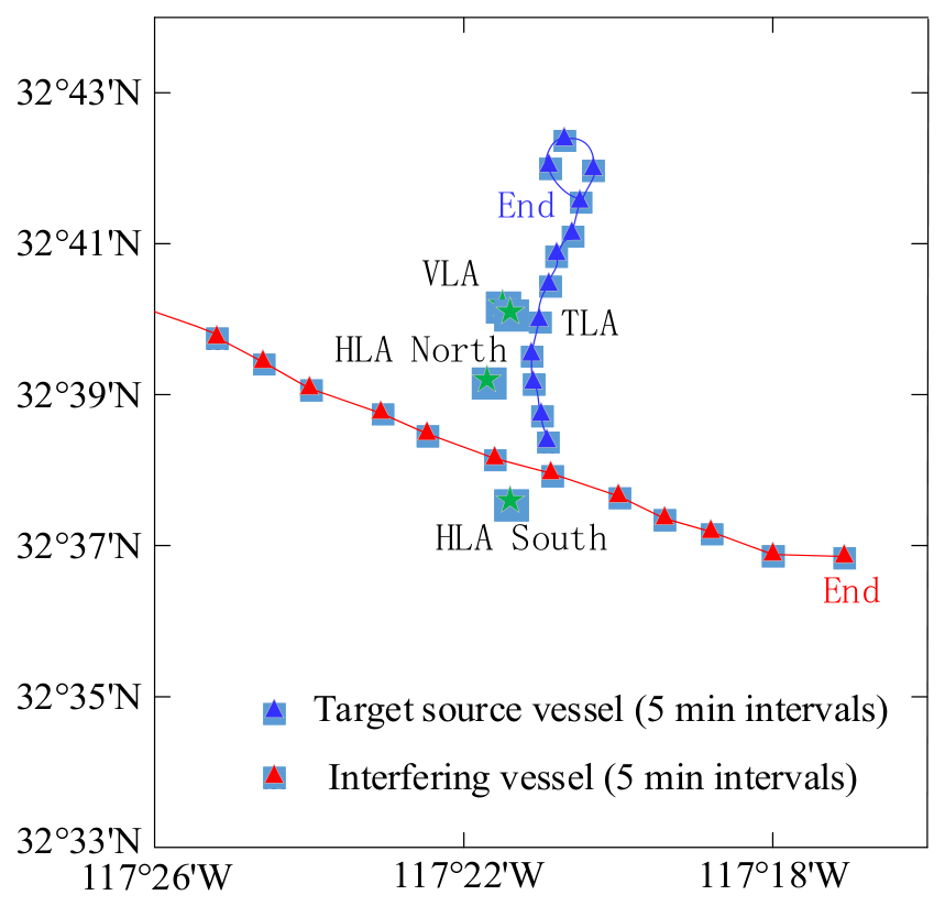
In Event S59, the target source vessel traveled from south to north at approximately 2.5 m/s along the 180 m isobath east of the arrays, while the loud interfering vessel approached from the west and proceeded southeast between the two HLAs. The source vessel towed J-15, which transmitted tonal and broadband signals from 49 to 400 Hz, and J-13, which transmitted nine tones between 109 and 385 Hz. The full event lasts approximately 3900 s. Both the narrowband and broadband analyses use 151 non-overlapping 1 s segments with start times from 2400 to 2550 s, inclusive. The time interval and channel subset were adopted as fixed case-study selections, and sensitivity to these choices was not investigated. Figure 13 shows both vessel tracks and the four array locations.

Before DOA processing, all selected channels were filtered using the same 512th-order FIR bandpass filter with cutoff frequencies of 20 and 1000 Hz. No additional channel-dependent calibration was applied. The subsequent narrowband and broadband analyses used 64 Hz and 49–400 Hz, respectively.

5.2. Data Processing and Analysis

5.2.1. Narrowband Data Processing

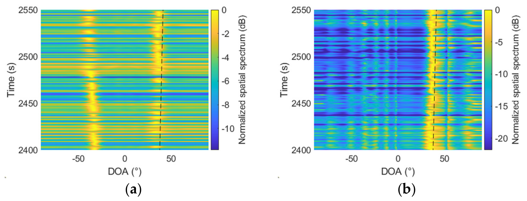
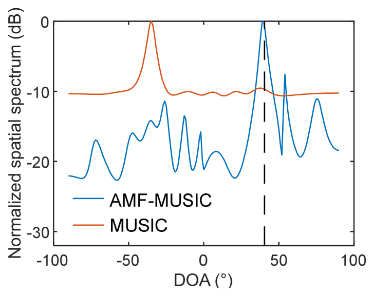
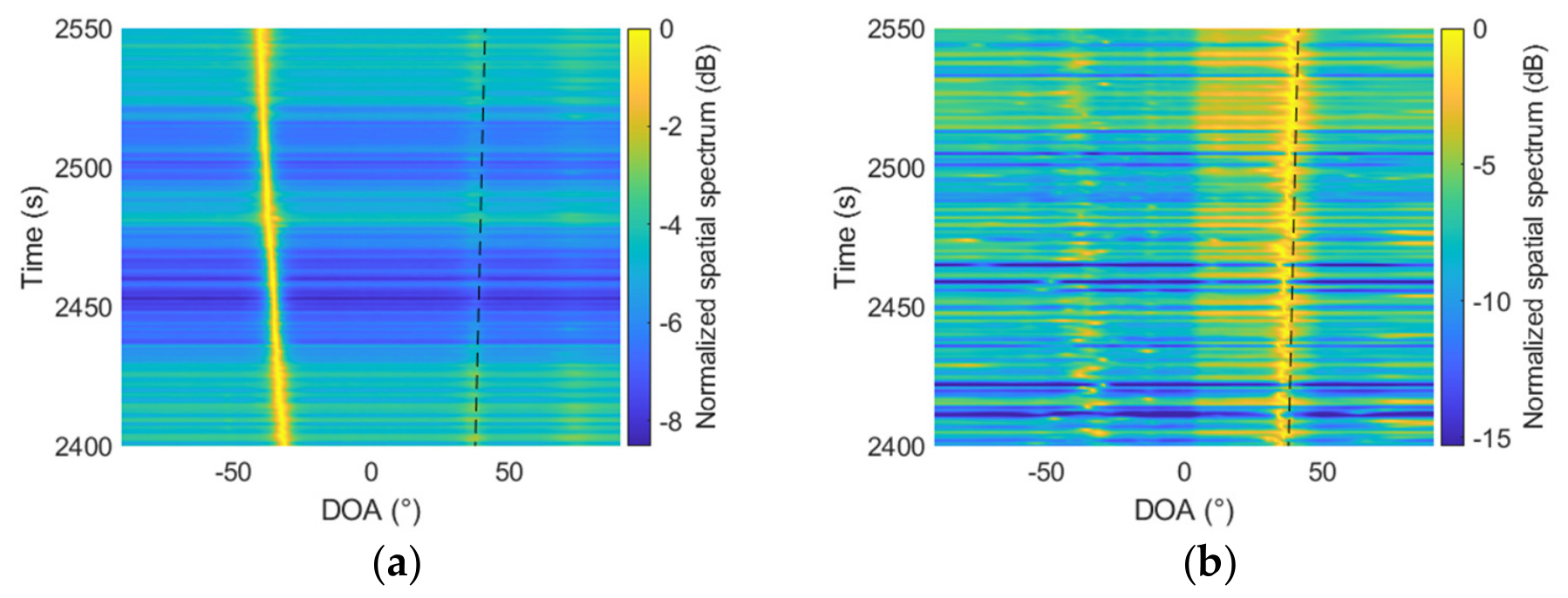
The line spectrum signal with a frequency of 64 Hz was selected for narrowband processing. The selected channels were first bandpass filtered over 20–1000 Hz as described in Section 5.1. The 64 Hz component was then used for narrowband processing with non-overlapping 1 s segments sampled at 3276.8 Hz. Figure 14 shows the DOA-time histories obtained by MUSIC without interference suppression and by MUSIC after narrowband AMF-based interference suppression. The dotted line in Figure 14 represents the GPS-derived ground-truth target DOA over time.

Figure 14 shows that AMF processing suppresses the interference-related responses and makes the target ridge more prominent. For each frame, the strongest local maxima within 25–45° and −50° to −20° were associated with the target and interference, respectively. A frame was considered invalid if no local maximum was found in either region and was excluded from the corresponding statistics. All 151 frames were valid for both MUSIC and AMF-MUSIC. The interference DOA obtained from the MUSIC spectrum was used as a common reference for both methods, and the spatial-spectrum SIR was defined as the difference, in dB, between the spectrum levels at the associated target and interference DOAs. As shown in

Table 3. Narrowband DOA-estimation errors and mean spatial-spectrum SIRs for MUSIC and AMF-MUSIC over 151 one-second SWellEx-96 data frames.

Method	RMSE (°)	MAE (°)	Mean Spatial-Spectrum SIR (dB)	Valid Frames
MUSIC	11.16	5.93	−0.41	151/151
AMF-MUSIC	5.18	4.18	13.18	151/151

, AMF-MUSIC reduced the RMSE from 11.16° to 5.18° and the MAE from 5.93° to 4.18°, while increasing the mean spatial-spectrum SIR from −0.41 dB to 13.18 dB.

Figure 15 compares the spatial spectra for the segment beginning at $t=2460$ s. Conventional MUSIC does not place its dominant peak near the ground-truth target DOA, whereas AMF-MUSIC suppresses the dominant interference response and produces a peak near that bearing. The remaining isolated maxima in Figure 15 do not form temporally persistent ridges in the DOA–time history shown in Figure 14. Therefore, this single-segment result is interpreted as a representative example rather than as an independently validated detection.

5.2.2. Broadband Data Processing

The broadband analysis used the same 151 non-overlapping 1 s data segments as the narrowband analysis. Each segment contained 3277 samples at a sampling frequency of 3276.8 Hz and was processed using a 3277-point DFT with a rectangular window; no temporal overlap or additional zero-padding was applied. The 49–400 Hz analysis band was divided into 36 non-overlapping narrow subbands with a nominal bandwidth of 10 Hz. The uppermost subband was truncated at the 400 Hz boundary. Each subband was represented by its center frequency for steering-vector construction and AMF design.

Let ${\mathcal{B}}_b$ denote the set of DFT bins contained in the $b$-th subband, $K_b$ the number of frequency bins in that subband, and ${\mathbf{x}}_m\left(f_k\right)$ the vector of multichannel DFT coefficients for the $m$-th data segment at frequency $f_k$. The sample cross-spectral matrix for the $b$-th subband was estimated by averaging the outer-product spectral matrices over all DFT bins within that subband:

$${\widehat{\mathbf{R}}}_{m,b}={\displaystyle \frac{1}{K_b}}\sum _{f_k\in {\mathcal{B}}_b}{\mathbf{x}}_m\left(f_k\right){\mathbf{x}}_m^H\left(f_k\right).$$

For each subband, a single steering matrix and AMF were constructed at the corresponding center frequency. A MUSIC spatial spectrum was then obtained separately for each subband. This procedure assumes that the variation of the array manifold within each 10 Hz subband is sufficiently small for the center-frequency narrowband approximation.

No subband-by-subband normalization was applied. The broadband spatial spectrum was formed by equal-weight summation of the linear spatial spectra obtained from the 36 subbands.

$$P_m^{\mathrm{B}\mathrm{B}}\left(\theta \right)={\displaystyle \sum _{b=1}^{36}}{P}_{m,b}\left(\theta \right).$$

The combined spectrum was normalized independently within each 1 s segment and subsequently converted to decibels.

Figure 16 shows the resulting broadband DOA-time histories obtained by MUSIC without interference suppression and by MUSIC after broadband AMF-based interference suppression. The dotted line denotes the GPS-derived ground-truth target DOA.

Figure 16 shows that, before interference suppression, the target trajectory in the MUSIC DOA-time histories is almost completely masked by strong interference. After broadband AMF processing, the target-related DOA ridge becomes more visible in the DOA-time histories and shows qualitative correspondence with the ground-truth target DOA. However, no framewise tracking-error or detection-probability metric was calculated, and Figure 16 therefore provides qualitative rather than quantitative evidence.

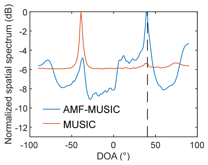
At t = 2520 s, the spatial spectra before and after interference suppression are compared, as shown in Figure 17.

Figure 17 shows that, at $t=2520$ s, AMF-MUSIC reduces the dominant interference-related response and produces a peak close to the ground-truth target DOA. The residual peaks in Figure 17 do not form persistent trajectories in the broadband DOA–time history shown in Figure 16 and may reflect subband-dependent spatial-response distortion. Because this is a single-segment example and no quantitative association metric was applied, the result is interpreted qualitatively.

6. Discussion

The controlled comparison indicates that the main benefit of the AMF is not uniformly stronger suppression, but a covariance-dependent allocation of suppression toward the dominant interferer while maintaining feasible passband fidelity. The contrast between the −25 and −40 dB CMF settings, together with the infeasibility of the tighter AMF constraint, shows that both filters remain constraint-sensitive. The observed advantage should therefore be interpreted as a more favorable configuration-dependent suppression–fidelity balance within the feasible region.

The SNR- and INR-dependent experiments use method-specific stopband bounds and therefore characterize the adopted configurations rather than isolate the effect of data dependence alone. Nevertheless, the relative stability of AMF-MUSIC with increasing INR is consistent with its covariance-dependent behavior. This advantage depends on accurate covariance estimation and steering vectors. The limited-snapshot experiment confirms that reduced sample support degrades target resolution, while nonstationary interference, steering-vector mismatch, and interference inside or near the passband were not quantified in the present study.

For coherent sources, FSS restores the covariance rank at the cost of a reduced effective aperture. The additional simulations considered subarray lengths of 20–23 sensors and target separations of 2–6°. The results show that the effect of subarray length is most pronounced near the resolution limit, reflecting the tradeoff between the retained effective aperture and the number of overlapping subarrays. All tested subarray configurations achieved resolution probabilities of at least 95% when the angular separation was 4.5° or greater. The limited-snapshot analysis further showed that the resolution probability increased from 0.390 with 50 snapshots to 0.980 with 5000 snapshots. Robustness to other coherence levels, source numbers, interference conditions, and model mismatch remains to be evaluated.

The basic full-dimensional AMF formulation follows [17]. In the proposed coherent-source processing chain, the FSS covariance matrix is used both to design the data-dependent AMF and to form the covariance matrix for subsequent MUSIC processing, whereas conventional FSS-MUSIC uses spatial smoothing primarily for covariance-rank restoration and subspace estimation. The broadband method in [19] also uses adaptive matrix filtering but combines it with sparse spectral fitting. Reference [21] reported an approximately 4 dB output signal-to-interference-ratio improvement under a different near-field interference configuration. Table 3 reports a spatial-spectrum SIR rather than a power-domain output SINR. Moreover, the array, source, and constraint settings differ from those in [21]; therefore, a direct numerical comparison is not appropriate. The present findings should therefore be interpreted within the investigated configurations rather than as evidence of universal superiority over prior methods.

The main computational burden arises from the convex AMF optimization, whose number of complex variables grows with the square of the sensor or subarray dimension. The 20-sensor AMF and the 21-sensor subarray AMF contain 400 and 441 complex variables, respectively. Broadband processing further repeats covariance estimation, AMF design, and MUSIC processing across frequency subbands. The current CVX/SDPT3 implementation is therefore suitable for offline or blockwise processing, but real-time feasibility has not been established because hardware-specific runtimes were not measured. Reduced update rates, parallel subband processing, smaller constraint grids, and structure-exploiting solvers may reduce the computational burden.

7. Conclusions

This study investigated covariance-dependent AMF spatial prefiltering for underwater acoustic DOA estimation under strong out-of-sector interference. Under the common −25 dB stopband bound, both CMF-MUSIC and AMF-MUSIC resolved the two non-coherent targets, while AMF-MUSIC produced a comparatively smoother out-of-sector background. Tightening the CMF bound reduced its background local maxima but degraded target resolution, demonstrating a tradeoff between stopband suppression and passband fidelity. Within its feasible constraint region, the AMF provided a more favorable balance by concentrating suppression near the actual interference direction through its covariance-dependent objective. However, the unequal-bound Monte Carlo results characterize the adopted configurations and do not isolate the effect of data dependence alone.

For coherent-source processing, the FSS covariance matrix was incorporated into both the AMF design and subsequent MUSIC processing. Simulations over target separations of 2–6° and subarray lengths of 20–23 sensors showed that subarray-length sensitivity is most pronounced near the resolution limit and that all tested subarray lengths achieved two-target resolution probabilities of at least 95% when the coherent-target angular separation was 4.5° or greater under the investigated SNR and INR conditions. For the SWellEx-96 data, AMF-MUSIC reduced the narrowband RMSE from 11.16° to 5.18° and increased the mean spatial-spectrum SIR from −0.41 dB to 13.18 dB, while the broadband results provided qualitative evidence of interference suppression. The limited-snapshot analysis further showed that the resolution probability increased from 0.390 with 50 snapshots to 0.980 with 5000 snapshots, demonstrating the sensitivity of AMF-FSS-MUSIC to the available sample support.

The present results do not establish universal robustness or real-time capability. Future work will include broader equal-constraint Monte Carlo comparisons, systematic constraint-sensitivity and model-mismatch analyses, broader measured-data validation, and reduced-complexity AMF implementation.

References

1. Fang, E.; Sun, C.; Gui, C. Self Noise-Reduction Method Based on Spatial Filtering for a Vector Flank Array Platform. J. Harbin Eng. Univ. 2020, 41, 1636–1641. (In Chinese) [Google Scholar] [CrossRef]
2. Wu, H.; Han, D.; Huang, X. Research on spatial matrix filtering data extraction of antenna array. Sci. Technol. Innov. Appl. 2021, 11, 1–4. (In Chinese) [Google Scholar]
3. Han, D.; Zhang, H. Spatial Matrix Filtering and Its Application; Science Press: Beijing, China, 2016. (In Chinese) [Google Scholar]
4. Liang, G.; Shi, Z.; Qiu, L.; Sun, S.; Lan, T. Sparse Bayesian Learning Based Direction-of-Arrival Estimation under Spatially Colored Noise Using Acoustic Hydrophone Arrays. J. Mar. Sci. Eng. 2021, 9, 127. [Google Scholar] [CrossRef] [Scilit]
5. Wang, W.; Li, X.; Zhang, K.; Shi, J.; Shi, W.; Ali, W. Robust Direction Finding via Acoustic Vector Sensor Array with Axial Deviation under Non-Uniform Noise. J. Mar. Sci. Eng. 2022, 10, 1196. [Google Scholar] [CrossRef] [Scilit]
6. Vaccaro, R.J.; Harrison, B.F. Optimal Matrix-Filter Design. IEEE Trans. Signal Process. 1996, 44, 705–709. [Google Scholar] [CrossRef] [Scilit]
7. Zhu, Z.; Wang, S.; Leung, H.; Ding, Z. Matrix Filter Design Using Semi-Infinite Programming with Application to DOA Estimation. IEEE Trans. Signal Process. 2000, 48, 267–271. [Google Scholar] [CrossRef]
8. MacInnes, C.S. Source Localization Using Subspace Estimation and Spatial Filtering. IEEE J. Ocean. Eng. 2004, 29, 488–497. [Google Scholar] [CrossRef]
9. Filiz, O.; Yener, A. Rank-Constrained Temporal-Spatial Matrix Filters for CDMA Systems. IEEE Trans. Wirel. Commun. 2004, 3, 1974–1979. [Google Scholar] [CrossRef]
10. Yan, S.; Ma, Y. Optimal Design and Verification of Temporal and Spatial Filters Using a Second-Order Cone Programming Approach. Sci. China Ser. F Inf. Sci. 2006, 49, 235–253. [Google Scholar] [CrossRef] [Scilit]
11. Zhang, D. Application of time domain broadband spatial matrix filter in ship noises separating area. In Proceedings of the 2021 OES China Ocean Acoustics (COA), Harbin, China, 14–17 July 2021; pp. 866–868. [Google Scholar] [CrossRef] [Scilit]
12. Zou, N.; Liu, G.; Fu, J.; Liang, G.; Qi, B.; Qiu, L.; Wang, Y.; Sun, S.; Li, C.; Li, X.; et al. Strong Interference Suppression Method Based on Spatial Matrix Filtering and Interference Cancellation. China Patent CN111273237A, 12 June 2020. (In Chinese) [Google Scholar]
13. Huang, X.; Chen, F.; Mo, S.; Wang, B. Fully Steerable and Interference Suppressible Differential Beamforming for Linear Acoustic Vector Sensor Array with Small Aperture. IEEE Trans. Instrum. Meas. 2025, 74, 9520915. [Google Scholar] [CrossRef] [Scilit]
14. Sun, S.-Y.; Zhang, L.; Dai, Z.-H.; Zhang, F.; Wang, F.-Y.; Yin, J.-W. Adaptive Nulling Array Direction-of-Arrival Estimation Based on Adaptive Kernel Width Mixture Correntropy under Impulsive Noise. J. Acoust. Soc. Am. 2025, 158, 4435–4449. [Google Scholar] [CrossRef] [Scilit] [PubMed]
15. Malyshkin, G.S. Experimental Testing of the Efficiency of Fast Projective Adaptive Algorithms. Acoust. Phys. 2019, 65, 749–764. [Google Scholar] [CrossRef] [Scilit]
16. Hassanien, A.; Abd Elkader, S.; Gershman, A.B.; Wong, K.M. Convex Optimization-Based Beam-Space Preprocessing with Improved Robustness against Out-of-Sector Sources. IEEE Trans. Signal Process. 2006, 54, 1587–1595. [Google Scholar] [CrossRef] [Scilit]
17. Feng, J.; Yang, Y.; Sun, C. Adaptive spatial matrix filter design with application to DOA estimation. J. Syst. Simul. 2007, 19, 4798–4802. (In Chinese) [Google Scholar] [CrossRef]
18. Liu, Z.; Sun, C.; Guo, G. Application of adaptive spatial matrix filter to matched field source localization. Acoust. Technol. 2010, 29, 573–578. (In Chinese) [Google Scholar]
19. Yang, Y.; Zhang, Y.; Yang, L. Wideband Sparse Spatial Spectrum Estimation Using Matrix Filter with Nulling in a Strong Interference Environment. J. Acoust. Soc. Am. 2018, 143, 3891–3898. [Google Scholar] [CrossRef] [Scilit] [PubMed]
20. Yang, P.; Zhou, W. Design and Experiment of Reduced-Dimension Adaptive Array Based on FIR Filters. IEEE Antennas Wirel. Propag. Lett. 2021, 20, 204–208. [Google Scholar] [CrossRef] [Scilit]
21. Lee, H.; Ahn, J.; Kim, Y.; Chung, J. Direction-of-Arrival Estimation of Far-Field Sources under Near-Field Interferences in Passive Sonar Array. IEEE Access 2021, 9, 28413–28420. [Google Scholar] [CrossRef] [Scilit]
22. Hamid, U.; Wyne, S.; Butt, N.R. Joint Model-Order and Robust DoA Estimation for Underwater Sensor Arrays. Sensors 2023, 23, 5731. [Google Scholar] [CrossRef] [Scilit] [PubMed]
23. Lin, B.; Hu, G.; Zhou, H.; Zheng, G. Coherent Signal DOA Estimation for MIMO Radar under Composite Background of Strong Interference and Non-Uniform Noise. Sensors 2022, 22, 9833. [Google Scholar] [CrossRef] [Scilit] [PubMed]
24. Qi, B.; Liu, X.; Dou, D.; Zhang, Y.; Hu, R. An Enhanced DOA Estimation Method for Coherent Sources via Toeplitz Matrix Reconstruction and Khatri–Rao Subspace. Electronics 2023, 12, 4268. [Google Scholar] [CrossRef] [Scilit]
25. Zhagypar, R.; Zhagyparova, K.; Akhtar, M.T. Spatially Smoothed TF-Root-MUSIC for DOA Estimation of Coherent and Non-Stationary Sources under Noisy Conditions. IEEE Access 2021, 9, 95754–95766. [Google Scholar] [CrossRef] [Scilit]
26. Wan, Z.; Liu, W. Time-Domain Wideband DOA Estimation under the Convolutional Sparse Coding Framework. IEEE Signal Process. Lett. 2022, 29, 274–278. [Google Scholar] [CrossRef] [Scilit]
27. Yao, J.; Zhao, C.; Bai, J.; Ren, Y.; Wang, Y.; Miao, J. Satellite Interference Source Direction of Arrival Estimation Based on Frequency-Domain Covariance Matrix Reconstruction. Sensors 2023, 23, 7575. [Google Scholar] [CrossRef] [Scilit] [PubMed]
28. Schmidt, R. Multiple Emitter Location and Signal Parameter Estimation. IEEE Trans. Antennas Propag. 1986, 34, 276–280. [Google Scholar] [CrossRef] [Scilit]
29. Wang, Y.; Chen, H.; Peng, Y. Spatial Spectrum Estimation Theory and Algorithm; Tsinghua University Press: Beijing, China, 2004. (In Chinese) [Google Scholar]
30. Murray, J.; Ensberg, D. The SWellEx-96 Experiment. Available online: https://swellex96.ucsd.edu/ (accessed on 23 July 2026).
Figure 1. Schematic of the forward spatial smoothing algorithm.
Jmse 14 01564 g001
Figure 2. Narrowband spatial-matrix-filter responses obtained using the Simulation 1 configuration in Table 2. Two non-coherent targets are located at the ground-truth DOAs of −2° and 1°, with an SNR of 0 dB for each target, while the interferer is located at 50° with an INR of 40 dB. (a) Amplitude responses of the CMF and AMF; (b) corresponding passband-response errors.
Jmse 14 01564 g002
Figure 3. Broadband AMF response for a target at 5° and an interferer at −40°. The target SNR is −10 dB, the INR is 20 dB, and both sources occupy the 900–1100 Hz band, which is divided into 20 Hz subbands. Surface colors represent the corresponding response levels in dB. (a) AMF amplitude response; (b) corresponding passband-response error.
Jmse 14 01564 g003
Figure 4. Controlled DOA-spectrum comparison using conventional MUSIC, CMF-MUSIC, and AMF-MUSIC for the same simulated array data. The targets are located at −2° and 1°, and the interferer is located at 50°. The dashed vertical lines denote the ground-truth target DOAs. CMF and AMF use the same −25 dB stopband bound: (a) full angular range; (b) enlarged target sector.
Jmse 14 01564 g004
Figure 5. Comparison of the DOA spatial spectra obtained using CMF-MUSIC and AMF-MUSIC for two non-coherent targets with ground-truth DOAs of 2 ° and 1 ° and an out-of-sector interferer located at 50 ° . The target SNR is −5 dB and the INR is 20 dB. CMF uses the −40 dB stopband bound and AMF uses the −25 dB stopband bound: (a) spatial spectra over the full angular range; (b) enlarged view of the passband containing the two ground-truth target DOAs.
Jmse 14 01564 g005
Figure 6. DOA-estimation performance of CMF-MUSIC and AMF-MUSIC over 200 Monte Carlo trials at each SNR from −15 to 15 dB in 2.5 dB increments, with the INR fixed at 20 dB. The ground-truth DOAs of Targets 1 and 2 are −2° and 1°, respectively, while the interference DOA is 50°. (a) Mean estimate for Target 1; (b) mean estimate for Target 2; (c) average target-wise RMSE; (d) average target-wise MAE; (e) two-target resolution probability. A trial is considered successfully resolved when two distinct peaks are detected and both paired DOA estimates have absolute errors not exceeding 1°.
Jmse 14 01564 g006aJmse 14 01564 g006b
Figure 7. DOA-estimation performance of CMF-MUSIC and AMF-MUSIC over 200 Monte Carlo trials at each INR from −5 to 25 dB in 2.5 dB increments, with the target SNR fixed at −10 dB. The ground-truth DOAs of Targets 1 and 2 are −2° and 1°, respectively, while the interference DOA is 50°. (a) Mean estimate for Target 1; (b) mean estimate for Target 2; (c) average target-wise RMSE; (d) average target-wise MAE; (e) two-target resolution probability. A trial is considered successfully resolved when two distinct peaks are detected and both paired DOA estimates have absolute errors not exceeding 1°.
Jmse 14 01564 g007
Figure 8. Spatial spectra obtained using AMF-MUSIC and AMF-FSS-MUSIC in the coherent-source simulation. The two coherent targets have ground-truth DOAs of −2° and 3°, respectively, while the coherent interferer is located at 50°. The target SNR is −5 dB, and the INR is 20 dB. This figure presents a representative single simulation.
Jmse 14 01564 g008
Figure 9. Performance of AMF-FSS-MUSIC over 200 Monte Carlo trials at each SNR from −20 to 15 dB in 2.5 dB increments, with the INR fixed at 20 dB. The coherent targets are located at −2° and 3°, and the coherent interferer is located at 50°. (a) Mean estimate for Target 1; (b) mean estimate for Target 2; (c) average target-wise RMSE; (d) average target-wise MAE; (e) two-target resolution probability. A trial is considered successfully resolved when two distinct peaks are detected and both paired DOA estimates have absolute errors not exceeding 1°.
Jmse 14 01564 g009aJmse 14 01564 g009b
Figure 10. Performance of AMF-FSS-MUSIC for coherent-target angular separations from 2° to 6° in 0.5° increments and subarray lengths of 20, 21, 22, and 23 sensors over 200 paired Monte Carlo trials: (a) resolution probability; (b) conditional RMSE calculated from successfully resolved trials and reported only when the resolution probability was at least 0.5. A trial was considered successful when two distinct target peaks were detected and both absolute DOA errors were within 1°. The target SNR was −5 dB, the INR was 20 dB, and the normalized AMF stopband bound was −25 dB.
Jmse 14 01564 g010
Figure 11. Numerical evaluation of AMF-FSS-MUSIC under coherent-source conditions. (a) resolution-probability comparison with conventional FSS-MUSIC at different target angular separations; (b) corresponding conditional RMSE calculated from successfully resolved trials and reported only when the resolution probability was at least 0.5; (c) resolution probability of AMF-FSS-MUSIC for different numbers of snapshots. For (a,b), both methods use 21-element subarrays and process identical simulated data over 200 paired Monte Carlo trials at each target separation. For (c), the target separation is fixed at 5°, and 200 trials are performed for each snapshot number. The target SNR is −5 dB, the INR is 20 dB, and the coherent interferer is located at 50°.
Jmse 14 01564 g011
Figure 12. Corrected measured horizontal coordinates of the HLA South hydrophones. The x - and y -coordinates denote East and North positions in metres, respectively, relative to the official array-coordinate origin. Open blue circles indicate all 28 processed HLA South channels, while filled red circles indicate the selected processed channels 14–28, corresponding to physical elements 17–30 and 32. The labels “14” and “28” are processed-channel numbers and indicate the endpoints and ordering of the selected subset.
Jmse 14 01564 g012
Figure 13. Geographic tracks of the target source vessel and interfering vessel during SWellEx-96 Event S59. The horizontal and vertical coordinates represent longitude and latitude, respectively. Blue triangles denote the target source vessel, and red triangles denote the interfering vessel; successive triangular markers are separated by five-minute intervals. The first marker on each track indicates its start location, while “End” identifies its final location. Cyan stars indicate the vertical line array (VLA), tilted line array (TLA), HLA North, and HLA South.
Jmse 14 01564 g013
Figure 14. Narrowband DOA-time histories obtained from SWellEx-96 Event S59 using HLA South processed channels 14–28, 1 s data segments, and the 64 Hz tonal component over the 2400–2550 s interval: (a) MUSIC without spatial prefiltering; (b) AMF-MUSIC after interference suppression. The color represents the normalized spatial-spectrum level in dB, and the dotted line denotes the GPS-derived target DOA.
Jmse 14 01564 g014
Figure 15. Narrowband spatial spectra obtained from a 1 s SWellEx-96 data segment at t = 2460 s using the 64 Hz tonal component: MUSIC without spatial prefiltering and AMF-MUSIC after interference suppression. The dotted line denotes the GPS-derived target DOA. This is a representative single-segment result.
Jmse 14 01564 g015
Figure 16. Broadband DOA-time histories obtained from SWellEx-96 Event S59 using HLA South processed channels 14–28, 1 s data segments, and the 49–400 Hz processing band over the 2400–2550 s interval: (a) MUSIC without spatial prefiltering; (b) AMF-MUSIC after interference suppression. The color represents the normalized spatial-spectrum level in dB, and the dotted line denotes the GPS-derived target DOA.
Jmse 14 01564 g016
Figure 17. Broadband spatial spectra obtained from a 1 s SWellEx-96 data segment at t = 2520 s over the 49–400 Hz processing band: MUSIC without spatial prefiltering and AMF-MUSIC after interference suppression. The dotted line denotes the GPS-derived target DOA. This is a representative single-segment result.
Jmse 14 01564 g017