Uncertainty-Weighted Robust Frequency-Scanning AVO Inversion for Fluid Prediction in Marine Low-Permeability Gas-Bearing Sandstones: A Case Study from the Xihu Sag, East China Sea

Abstract

Marine low-permeability gas-bearing sandstones are commonly characterized by thin sand–mud interbeds, poor reservoir properties, limited seismic bandwidth, and heterogeneous pore structures and fluid distributions, which make stable fluid prediction from conventional prestack seismic attributes difficult. This study proposes an uncertainty-weighted robust frequency-scanning amplitude variation with offset (AVO) inversion method, termed URFS-AVO, for gas-bearing sandstone identification in the Xihu Sag, East China Sea. Under a fluid-matrix decoupled AVO framework, a frequency-dependent P-to-P (PP) reflection-coefficient equation related to the fluid bulk modulus is combined with matching-pursuit Wigner–Ville distribution (MP-WVD) spectral decomposition to obtain local time–frequency spectra from prestack angle gathers. Moving narrow frequency windows are then used to estimate local fluid-dispersion attributes within the effective seismic bandwidth. Rather than extracting the maximum response, URFS-AVO fuses multi-window estimates using local inversion uncertainty and frequency-domain consistency. Tests based on the Chapman pore–microcrack model and the generalized propagator matrix show that the proposed attribute is sensitive to gas-bearing variations. Compared with maximum-window frequency-scanning AVO (FS-AVO), URFS-AVO produces a more focused target-layer response and suppresses unstable background fluctuations, especially under noisy conditions. Application to marine prestack seismic data from the Xihu Sag shows that high URFS-AVO responses are generally consistent with gas-bearing intervals interpreted from well logs. The method provides a stable seismic constraint for fluid prediction in marine low-permeability gas-bearing sandstone reservoirs.

1. Introduction

Low-permeability gas-bearing sandstones in the Xihu Sag of the East China Sea are important marine hydrocarbon targets. The Huagang Formation reservoirs in the central anticlinal belt are commonly deeply buried and are characterized by thin sand–mud interbeds, low porosity, low permeability, and strong lateral heterogeneity. Public geological studies of analogous Huagang Formation reservoirs indicate that favorable channel sand bodies, hydrocarbon charging, and dissolution modification jointly control the development of high-quality reservoir intervals [1]. These geological controls generate strong spatial variability in pore structure and fluid distribution, which complicates seismic fluid discrimination in thinly interbedded low-permeability sandstone reservoirs [2,3,4,5,6,7]. Therefore, the key technical problem addressed in this study is how to extract a stable fluid-sensitive seismic response from marine prestack data affected by thin-bed tuning, heterogeneous reservoir properties, and limited bandwidth.

Amplitude variation with offset (AVO) analysis provides a theoretical basis for linking angle-dependent seismic amplitudes with subsurface elastic properties and fluid effects. Classical PP-wave reflection-coefficient approximations express amplitude variation in terms of P-wave velocity, S-wave velocity, and density perturbations [8]. Later formulations introduced Lamé parameters, bulk modulus, shear modulus, and related elastic combinations to improve lithology and fluid interpretation [9,10,11]. From the viewpoint of porous-rock physics, Russell et al. decomposed the elastic response into solid- and fluid-related terms and introduced AVO approximations involving the Gassmann fluid term [12,13]. Zong et al. developed stable fluid-factor inversion for heterogeneous reservoirs [14], and Yin and Zhang proposed an effective pore–fluid bulk modulus inversion method based on a fluid-matrix decoupled AVO approximation [15]. These studies promoted the development of rock-physics-constrained AVO fluid prediction. However, conventional elastic AVO inversion is usually based on a frequency-independent assumption, and its results may still be affected by lithology, pore structure, pressure state, layer thickness, and seismic bandwidth.

Seismic waves propagating through fluid-bearing porous rocks may exhibit velocity dispersion and attenuation. Such frequency-dependent responses are commonly associated with wave-induced fluid flow, squirt flow, patchy saturation, fracture-related pressure relaxation, and scattering in heterogeneous pore systems [16,17,18,19,20]. Frequency-dependent AVO inversion uses the variation in reflection amplitudes with frequency and angle to estimate dispersion attributes for hydrocarbon detection. Wilson et al. introduced frequency dependence into the AVO framework and estimated P-wave velocity dispersion from frequency-dependent reflection amplitudes [21]. Zhang et al. proposed a dispersion-dependent attribute for hydrocarbon detection [22]. Recent developments in frequency-dependent AVO inversion have focused mainly on improving the resolution and stability of time–frequency spectral decomposition [23,24], constructing more fluid-sensitive dispersion attributes [25], and extending frequency-dependent inversion to anisotropic and azimuthal reservoir characterization [26,27,28]. These advances improve the extraction and interpretation of local dispersion responses. However, reliably combining the estimates obtained from multiple overlapping frequency-scanning windows remains a practical issue. These studies show that prestack seismic data contain joint amplitude-angle–frequency information that can supplement conventional elastic attributes in fluid prediction.

Recent uncertainty analysis studies have estimated predictive uncertainty in AVO inversion using Bayesian-dropout deep learning [29] and characterized posterior uncertainty in prestack seismic inversion through Bayesian sampling based on Markov chain Monte Carlo (MCMC) methods [30]. These studies demonstrate the value of uncertainty information for evaluating inversion reliability; in URFS-AVO, however, the estimated local variance is used more narrowly as a relative reliability measure for combining overlapping frequency-window estimates rather than as a complete posterior uncertainty characterization.

Stable estimation of dispersion attributes remains difficult in marine low-permeability sandstone reservoirs. First, velocity dispersion attributes reflect the overall frequency-dependent response of saturated rock and may be influenced by the rock frame, pore structure, and non-fluid factors. Second, conventional fixed-window frequency-dependent inversion relies on a selected reference frequency and a relatively broad analysis band. When the target-layer dispersion curve is nonlinear, the effective seismic bandwidth is uneven, or spectral energy is weak at some frequencies, the local linear assumption used in the inversion may be weakened. Third, moving-window frequency scanning can reduce the dependence on a fixed reference frequency, but direct maximum-window extraction may amplify isolated anomalous windows caused by low wavelet energy, thin-bed tuning, spectral-estimation errors, or local ill-conditioned inversion [28]. This problem is particularly relevant for marine prestack seismic data, where far-angle amplitudes and high-frequency components are commonly less stable.

To improve the reliability of fluid prediction in marine low-permeability gas-bearing sandstones, this study develops an uncertainty-weighted robust frequency-scanning AVO inversion method. The method first constructs a frequency-dependent reflection-coefficient equation related to the fluid bulk modulus under a fluid-matrix decoupled AVO framework. Matching-pursuit Wigner–Ville distribution spectral decomposition is used to obtain high-resolution local time–frequency spectra from prestack angle gathers. A moving narrow-window frequency-scanning strategy is then applied within the effective seismic bandwidth to estimate local fluid-dispersion attributes. Finally, the local estimates are combined using weights derived from their estimated inversion variance, while the fused magnitude is modulated by a cross-window polarity-consistency factor. The principal methodological contribution of URFS-AVO therefore lies in the reliability- and polarity-aware fusion of local frequency-window estimates rather than in the separate use of fluid-matrix decoupling, MP-WVD spectral decomposition, or frequency scanning. Unlike maximum-window FS-AVO, which retains only the strongest local response, URFS-AVO reduces the influence of a single high-amplitude but poorly constrained estimate and suppresses the fused response when the reliable local estimates exhibit conflicting polarities.

The practical idea behind the proposed method can be summarized as follows. A gas-bearing interval may produce prestack amplitude variations that depend on both incidence angle and frequency. Frequency scanning therefore repeats the dispersion inversion over a series of narrow frequency windows, producing several local estimates at each time sample. Conventional maximum-window FS-AVO retains the strongest estimate, whereas URFS-AVO combines the local estimates according to their inversion uncertainty and cross-window polarity consistency. The final attribute is consequently less dependent on a single selected window and can be interpreted as a reliability-weighted measure of the fluid-related dispersion response.

The workflow of this study is organized as follows. First, the regional geological setting of the study area is summarized to define the reservoir type and seismic prediction problem. Second, the URFS-AVO method is formulated, including the fluid-matrix decoupled AVO approximation, wavelet-compensated frequency-domain inversion, MP-WVD spectral decomposition, local frequency scanning, and uncertainty-weighted fusion. Third, theoretical tests based on the Chapman pore–microcrack model and the generalized propagator matrix are conducted to analyze the gas-saturation-dependent elastic response, frequency-dependent reflection spectra, synthetic gathers, and inversion stability. Fourth, maximum-window FS-AVO and URFS-AVO attributes are compared under noise-free and noisy conditions. Finally, the proposed method is applied to marine prestack seismic data from the Xihu Sag and compared with gas-bearing intervals interpreted from well logs.

2. Geological Setting

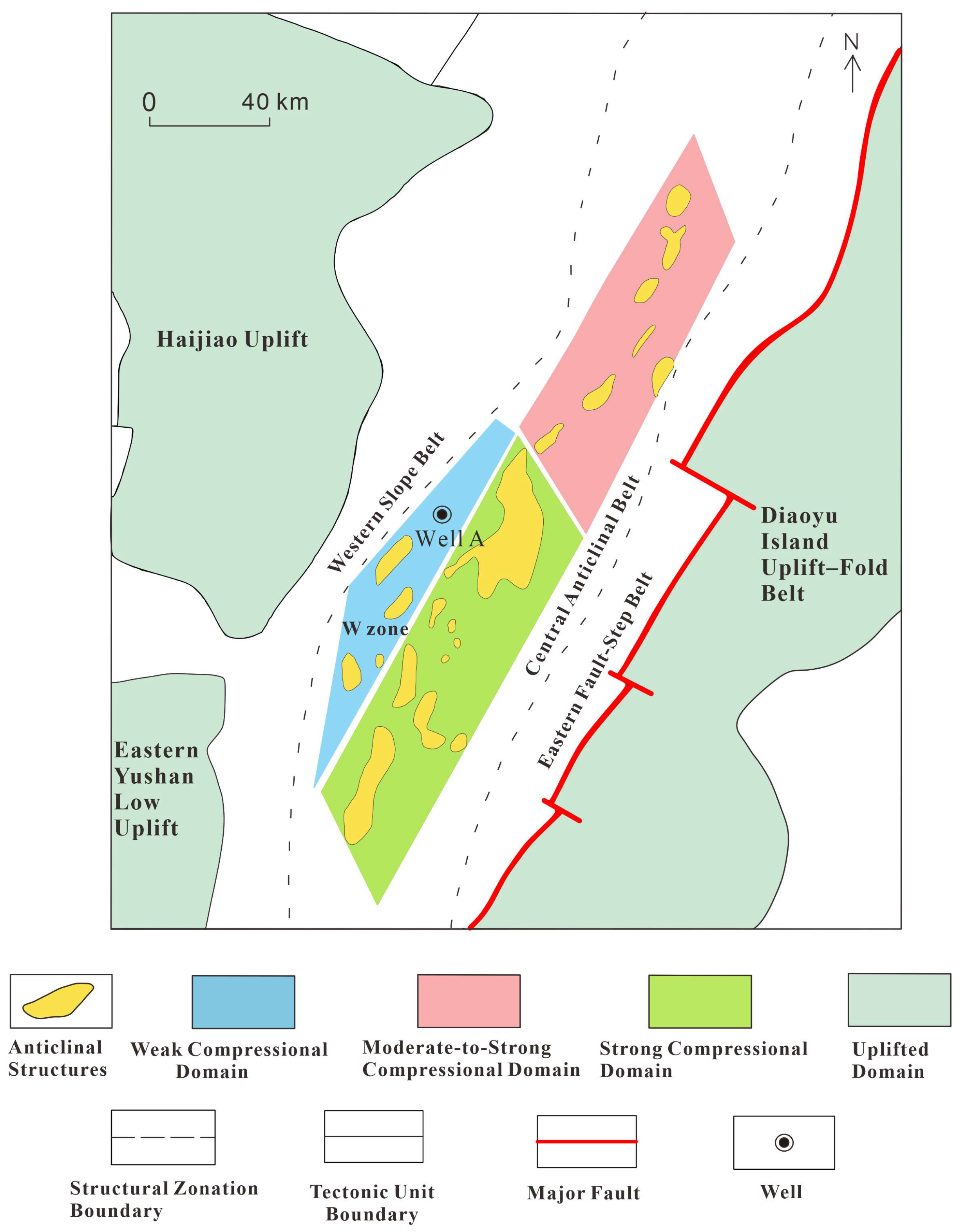
The study area is located in the Xihu Sag of the East China Sea Shelf Basin. The Xihu Sag is a Cenozoic petroliferous depression with several NE-trending structural belts, including the Western Slope Belt, the Central Anticlinal Belt, and the Eastern Fault-Steep Belt (Figure 1). The Central Anticlinal Belt lies between the Western Slope Belt and the Diaoyu Island Uplift-Fold Belt. Regional tectonic evolution includes an early fault-depression stage, a fault-depression transition stage, and a later regional subsidence stage. These stages controlled the present structural framework and the distribution of the major Cenozoic stratigraphic units [1].

The target interval is the Oligocene Huagang Formation. As summarized in

Table 1. Simplified Cenozoic stratigraphic framework and regional depositional settings relevant to the target Huagang Formation in the Xihu Sag.

Era		Formation	Depositional Setting
Quaternary		Donghai	Offshore and fluvial settings
Neogene	Pliocene	Santan
	Miocene	Liulang	Coastal to offshore settings
		Yuquan
		Longjing
Paleogene	Oligocene	Huagang	Spatially variable fluvial–deltaic and lacustrine systems with local transgressive and tidal influence
	Eocene	Pinghu	Tidal-flat and fluvial systems in a marine–continental transitional setting

, the principal Cenozoic stratigraphic units relevant to this study comprise, from bottom to top, the Pinghu Formation, Huagang Formation, Longjing Formation, Yuquan Formation, Liulang Formation, Santan Formation, and Donghai Group. The Huagang Formation overlies the Pinghu Formation and was deposited during the depression stage.

Regional studies indicate that the depositional environments of the Huagang Formation were spatially heterogeneous. Fluvial-deltaic and lacustrine deposits were widespread, and channel sand bodies constitute the principal reservoirs in the Central Anticlinal Belt [1]. However, at least two major transgressive episodes have been reported during Huagang deposition [31]. The earlier transgression was accompanied by enhanced tidal influence and the development of tide-influenced deltaic-to-estuarine systems in parts of the Xihu Sag [31,32]. Restricted-bay and tide-dominated depositional systems have also been documented locally in the Central Anticlinal Belt [33]. The Huagang Formation is therefore interpreted here as a spatially variable continental-to-marginal-marine succession rather than as a uniformly lacustrine or marine unit. Accordingly, this study is situated in an offshore marine-geophysical setting, whereas the depositional origin of the target Huagang interval is interpreted within this spatially variable continental-to-marginal-marine framework.

3. Methods

3.1. Fluid-Matrix Decoupled AVO Approximation

The proposed method starts from a fluid-matrix decoupled AVO approximation. For a weak-contrast interface, the PP-wave reflection coefficient can be expressed in terms of the Gassmann fluid term $\mathit{f}$, shear modulus $\mu$, and density $\rho$ [12,13]:

$$\begin{array}{c}{R}_{\mathrm{PP}}(\theta )=A(\theta ){\displaystyle \frac{\Delta f}{f}}+B(\theta ){\displaystyle \frac{\Delta \mu }{\mu }}+C(\theta ){\displaystyle \frac{\Delta \rho }{\rho }}.\end{array}$$

(1)

In Equation (1), $R_{\mathrm{PP}}(\theta )$ is the PP-wave reflection coefficient, $\theta$ is the average of the incident and transmitted angles, and $\Delta$ denotes the difference between the parameters across the interface. The angle-dependent coefficients are written as

$$\begin{array}{l}A(\theta )=\left(1-{\displaystyle \frac{{\gamma }_{\mathrm{dry}}^2}{{\gamma }_{\mathrm{sat}}^2}}\right){\displaystyle \frac{{\sec }^2\theta }{4}},\hfill \\ B(\theta )={\displaystyle \frac{{\gamma }_{\mathrm{dry}}^2}{4{\gamma }_{\mathrm{sat}}^2}}{\sec }^2\theta -{\displaystyle \frac{2}{{\gamma }_{\mathrm{sat}}^2}}{\sin }^2\theta ,\hfill \\ C(\theta )={\displaystyle \frac{1}{2}}-{\displaystyle \frac{{\sec }^2\theta }{4}}.\hfill \end{array}$$

(2)

Here, ${\gamma }_{\mathrm{dry}}=V_{P,\mathrm{dry}}/V_{S,\mathrm{dry}}$ and ${\gamma }_{\mathrm{sat}}=V_{P,\mathrm{sat}}/V_{S,\mathrm{sat}}$ are the P- to S-wave velocity ratios of the dry frame and saturated rock, respectively. The Gassmann fluid term can be calculated from the saturated-rock velocities and density as

$$\begin{array}{c}f=\rho \left(V_P^2-{\gamma }_{\mathrm{dry}}^2{V}_S^2\right).\hspace{1em}\hspace{1em}\end{array}$$

(3)

Following the Han–Batzle fluid-matrix decoupling relationship, the Gassmann fluid term can be written as the product of a porosity-dependent gain function and the effective pore–fluid bulk modulus $K_f$ [15,25,34]:

$$\begin{array}{c}f\approx G(\varphi )K_f,\hspace{1em}\hspace{1em}G(\varphi )={\displaystyle \frac{{\left(1-K_{\mathrm{dry}}/K_0\right)}^2}{\varphi }},\end{array}$$

(4)

where $\varphi$ is porosity, $K_{\mathrm{dry}}$ is the dry-frame bulk modulus, and $K_0$ is the mineral-grain bulk modulus. In practical implementation, the critical-porosity approximation can be used to simplify the gain function [35]:

$$\begin{array}{c}G(\varphi )\approx {\displaystyle \frac{\varphi }{{\varphi }_c^2}},\end{array}$$

(5)

where ${\varphi }_c$ is critical porosity. Combining Equations (4) and (5) first gives $f\approx \varphi K_f/{\varphi }_c^2$. Treating ${\varphi }_c$ as a fixed critical-porosity parameter and neglecting second-order products of the weak interfacial contrasts, the corresponding first-order relative perturbation is $\Delta f/f\approx \Delta K_f/K_f+\Delta \varphi /\varphi$. Moreover, because $f_m=\mu \varphi$, or equivalently $\mu =f_m/\varphi$, its first-order relative perturbation can be written as $\Delta \mu /\mu \approx \Delta f_m/f_m-\Delta \varphi /\varphi$. Substituting these two relationships into Equation (1) gives the fluid-matrix decoupled PP-wave reflection coefficient:

$$\begin{array}{c}{R}_{\mathrm{PP}}(\theta )=A(\theta ){\displaystyle \frac{\Delta K_f}{K_f}}+B(\theta ){\displaystyle \frac{\Delta f_m}{f_m}}+C(\theta ){\displaystyle \frac{\Delta \rho }{\rho }}+D(\theta ){\displaystyle \frac{\Delta \varphi }{\varphi }},\end{array}$$

(6)

Here, $f_m$ denotes the solid-rigidity parameter. After the preceding substitutions, the fluid-related term contributes $A(\theta )\Delta \varphi /\varphi$, whereas the solid-rigidity term contributes $-B(\theta )\Delta \varphi /\varphi$. Therefore, the coefficient of the porosity perturbation is $D(\theta )=A(\theta )-B(\theta )$. Substituting the expressions for $A(\theta )$ and $B(\theta )$ in Equation (2) gives

$$\begin{array}{c}D(\theta )={\displaystyle \frac{{\sec }^2\theta }{4}}-{\displaystyle \frac{{\gamma }_{\mathrm{dry}}^2}{2{\gamma }_{\mathrm{sat}}^2}}{\sec }^2\theta +{\displaystyle \frac{2}{{\gamma }_{\mathrm{sat}}^2}}{\sin }^2\theta .\end{array}$$

(7)

Equation (6) is used as the AVO parameterization for the subsequent frequency-scanning inversion. In addition, Equations (3) and (4) provide a direct way to estimate the fluid-bulk-modulus-related response from saturated-rock parameters:

$$\begin{array}{c}{K}_f(\omega )\approx {\displaystyle \frac{F(\omega )}{G(\varphi )}}={\displaystyle \frac{\rho (\omega )\left[V_P^2(\omega )-{\gamma }_{\mathrm{dry}}^2{V}_S^2(\omega )\right]}{G(\varphi )}}.\end{array}$$

(8)

This relationship is used in the rock-physics sensitivity analysis to compare the frequency-dependent response of the fluid-bulk-modulus-related term with that of P-wave velocity.

3.2. Frequency-Dependent AVO Equation and Wavelet-Compensated Spectral Difference

Seismic waves propagating through fluid-bearing porous rocks can induce local fluid-pressure relaxation and frequency-dependent reflection responses. Assuming that $K_f$ and $f_m$ vary with frequency, while $\rho$ and $\varphi$ are approximately frequency-independent within the local seismic band, Equation (6) can be extended to the frequency domain as

$$\begin{array}{c}{R}_{\mathrm{PP}}(\theta ,\omega )=A(\theta ){\displaystyle \frac{\Delta K_f}{K_f}}(\omega )+B(\theta ){\displaystyle \frac{\Delta f_m}{f_m}}(\omega )+C(\theta ){\displaystyle \frac{\Delta \rho }{\rho }}+D(\theta ){\displaystyle \frac{\Delta \varphi }{\varphi }}.\end{array}$$

(9)

For a reference frequency ${\omega }_0$, a first-order Taylor expansion of Equation (9) gives

$$\begin{array}{l}{R}_{\mathrm{PP}}(\theta ,\omega )\approx R_{\mathrm{PP}}(\theta ,{\omega }_0)+(\omega -{\omega }_0)A(\theta ){\displaystyle \frac{\partial }{\partial \omega }}\left({\displaystyle \frac{\Delta K_f}{K_f}}\right)\hfill \\ \hspace{1em}\hspace{1em}+(\omega -{\omega }_0)B(\theta ){\displaystyle \frac{\partial }{\partial \omega }}\left({\displaystyle \frac{\Delta f_m}{f_m}}\right).\hspace{1em}\hspace{1em}\hfill \end{array}$$

(10)

Equation (10) is obtained by applying a first-order Taylor expansion to the frequency-dependent terms around the reference frequency ${\omega }_0$. Within each local frequency window, the angle-dependent coefficients are treated as constants, the density- and porosity-related terms are assumed to be approximately frequency-independent, and higher-order terms are neglected. Substituting the dispersion attributes defined in Equation (11) into this first-order expansion gives Equation (12).

The fluid-bulk-modulus-related dispersion attribute and the solid-rigidity-related dispersion attribute are defined as

$$\begin{array}{c}{D}_{K_f}={\displaystyle \frac{\partial }{\partial \omega }}\left({\displaystyle \frac{\Delta K_f}{K_f}}\right),\hspace{1em}\hspace{1em}{D}_{f_m}={\displaystyle \frac{\partial }{\partial \omega }}\left({\displaystyle \frac{\Delta f_m}{f_m}}\right).\end{array}$$

(11)

The frequency-difference reflection coefficient is therefore

$$\begin{array}{c}\Delta R_{\mathrm{PP}}(\theta ,\omega )=R_{\mathrm{PP}}(\theta ,\omega )-R_{\mathrm{PP}}(\theta ,{\omega }_0)=(\omega -{\omega }_0)\left[A(\theta )D_{K_f}+B(\theta )D_{f_m}\right].\end{array}$$

(12)

The observed prestack seismic spectrum is not the reflection coefficient itself but the product of the wavelet spectrum $W(\omega )$ and the reflection coefficient. According to the convolution model,

$$\begin{array}{c}S(\theta ,\omega )=W(\omega )R_{\mathrm{PP}}(\theta ,\omega ).\end{array}$$

(13)

Following the conventional frequency-spectrum difference treatment used in frequency-dependent AVO inversion, the seismic spectral difference can be expressed by multiplying the reflection-coefficient difference by the wavelet spectrum at the analyzed frequency:

$$\begin{array}{l}\Delta S(\theta ,\omega )=S(\theta ,\omega )-S(\theta ,{\omega }_0) =(\omega -{\omega }_0)W(\omega )\left[A(\theta )D_{K_f}+B(\theta )D_{f_m}\right].\hfill \end{array}$$

(14)

For a prestack data set containing $n$ incidence angles and $m$ analyzed frequency samples, Equation (14) can be expanded into the following matrix form:

$$\left[\begin{array}{c}\Delta S({\theta }_1,{\omega }_1)\\ ⋮\\ \Delta S({\theta }_1,{\omega }_m)\\ ⋮\\ \Delta S({\theta }_n,{\omega }_1)\\ ⋮\\ \Delta S({\theta }_n,{\omega }_m)\end{array}\right]\left[\begin{array}{cc}({\omega }_1-{\omega }_0)W({\omega }_1)A({\theta }_1)& ({\omega }_1-{\omega }_0)W({\omega }_1)B({\theta }_1)\\ ⋮& ⋮\\ ({\omega }_m-{\omega }_0)W({\omega }_m)A({\theta }_1)& ({\omega }_m-{\omega }_0)W({\omega }_m)B({\theta }_1)\\ ⋮& ⋮\\ ({\omega }_1-{\omega }_0)W({\omega }_1)A({\theta }_n)& ({\omega }_1-{\omega }_0)W({\omega }_1)B({\theta }_n)\\ ⋮& ⋮\\ ({\omega }_m-{\omega }_0)W({\omega }_m)A({\theta }_n)& ({\omega }_m-{\omega }_0)W({\omega }_m)B({\theta }_n)\end{array}\right]\left[\begin{array}{c}{D}_{K_f}\\ D_{f_m}\end{array}\right].$$

(15)

Equation (15) can be simplified as

$$\begin{array}{c}d=Gm,\hspace{1em}\hspace{1em}m={\left[D_{K_f},D_{f_m}\right]}^T.\end{array}$$

(16)

The dispersion attribute vector is obtained by damped least squares:

$$\begin{array}{c}\widehat{m}={\left(G^{T}G+kI\right)}^{-1}{G}^{T}d,\end{array}$$

(17)

where $k$ is the damping factor and $I$ is the identity matrix. The first component of $\widehat{m}$ is the fluid-dispersion attribute $D_{K_f}$.

3.3. MP-WVD Time–Frequency Spectral Decomposition

Reliable dispersion-attribute inversion requires stable local time–frequency spectra of prestack seismic data. In this study, matching pursuit is combined with the Wigner–Ville distribution to obtain high-resolution time–frequency spectra [36,37]. Given a redundant dictionary $\mathcal{D}=g_{\lambda }(t)$, a seismic trace $s(t)$ can be decomposed as

$$\begin{array}{c}s(t)={\displaystyle \sum _{n=0}^{N-1}{a}_n}{g}_{{\lambda }_n}(t)+R_N(t).\end{array}$$

(18)

where $a_n$ is the coefficient of the $n$-th selected atom, $g_{{\lambda }_n}(t)$ is the best-matched atom, and $R_N(t)$ is the residual after $N$ iterations. At each iteration, the best atom is determined by

$$\begin{array}{l}{\lambda }_n=\underset{\lambda \in \mathcal{D}}{\arg \max }\left|〈R_n(t),g_{\lambda }(t)〉\right|,\hfill \\ a_n=〈R_n(t),g_{{\lambda }_n}(t)〉,\hfill \\ R_{n+1}(t)=R_n(t)-a_n{g}_{{\lambda }_n}(t).\hfill \end{array}$$

(19)

A Morlet atom is used to construct the redundant dictionary:

$$\begin{array}{c}{g}_{\lambda }(t)=C\exp \left[-\alpha {(t-\tau )}^2\right]\cos \left[2\pi f_c(t-\tau )+\phi \right],\hspace{1em}\hspace{1em}\lambda =(\tau ,f_c,\alpha ,\phi ).\end{array}$$

(20)

In Equation (20), $t$ denotes time, $C$ is the normalization factor, $\tau$ is the temporal center, $f_c$ is the center frequency of the atom, $\alpha$ controls its temporal width, $\phi$ is the phase, and $\lambda =(\tau ,f_c,\alpha ,\phi )$ is the atom-parameter vector. The angle brackets in Equation (19) denote the inner product, whereas the superscript $*$ in Equation (21) denotes complex conjugation. In Equation (21), $\tau$ is used as the integration-lag variable.

The Wigner–Ville distribution of a signal $s(t)$ is defined as

$$\begin{array}{c}{W}_s(t,\omega )={\displaystyle {\int }_{-\infty }^{+\infty }s}\left(t+{\displaystyle \frac{\tau }{2}}\right)s^{*}\left(t-{\displaystyle \frac{\tau }{2}}\right)e^{-i\omega \tau }d\tau .\end{array}$$

(21)

Instead of applying the Wigner–Ville distribution directly to the whole seismic trace, it is calculated for each selected atom and then summed to form the MP-WVD spectrum:

$$\begin{array}{c}{E}_s(t,\omega )={\displaystyle \sum _{n=0}^{N-1}|}{a}_n{|}^2{W}_{g_{{\lambda }_n}}(t,\omega ).\end{array}$$

(22)

The local amplitude spectrum $S(t,{\theta }_i,{\omega }_j)$ extracted from $E_s(t,\omega )$ is used as the input for frequency-scanning AVO inversion. The same spectral-decomposition parameters are applied to all angle stacks to preserve relative amplitude consistency among different incidence angles.

3.4. Frequency-Scanning AVO Inversion

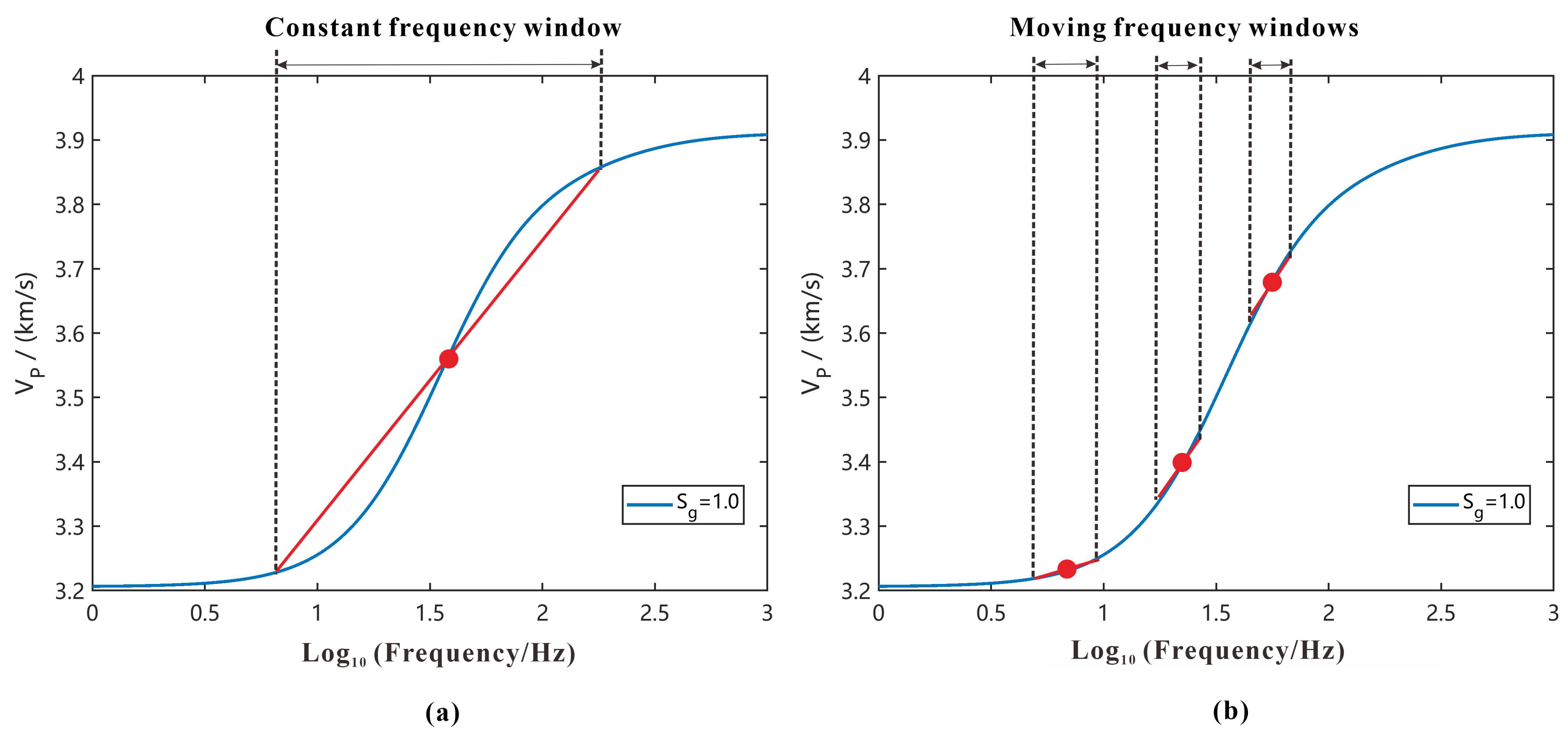
The frequency-scanning strategy uses multiple moving narrow windows within the reliable seismic bandwidth. Compared with a single fixed frequency window, the moving-window strategy improves the local validity of the first-order frequency expansion and reduces the dependence on a prescribed reference frequency (Figure 2). Within the effective frequency band $\mathcal{B}$, a series of scanning center frequencies ${\omega }_c$ are selected, and a local frequency window is defined as

$$\begin{array}{c}\Omega ({\omega }_c)=\left\{\omega :\left|\omega -{\omega }_c\right|\le h/2,\hspace{0.33em}\omega \in \mathcal{B}\right\},\end{array}$$

(23)

where $h$ denotes the full width of the local frequency window and $h/2$ is the corresponding half-width. For each ${\omega }_c$, the local spectral-difference data are defined as

$$\begin{array}{l}\begin{array}{l}\Delta S(\theta ,\omega ;{\omega }_c)=S(\theta ,\omega )-S(\theta ,{\omega }_c)\\ =(\omega -{\omega }_c)W(\omega )\left[A(\theta )D_{K_f}({\omega }_c)+B(\theta )D_{f_m}({\omega }_c)\right],\hspace{1em}\hspace{1em}\omega \in \Omega ({\omega }_c).\end{array}\hfill \end{array}$$

(24)

For each scanning window, the local spectral-difference data defined in Equation (24) can be written as a local matrix equation:

$$\begin{array}{c}d({\omega }_c)=G({\omega }_c)m({\omega }_c).\end{array}$$

(25)

where $d({\omega }_c)$ is composed of the local spectral differences $\Delta S({\theta }_i,{\omega }_j;{\omega }_c)$ and the two columns of $G({\omega }_c)$ are $({\omega }_j-{\omega }_c)W({\omega }_j)A({\theta }_i)$ and $({\omega }_j-{\omega }_c)W({\omega }_j)B({\theta }_i)$, respectively. The local solution is

$$\begin{array}{c}\widehat{m}({\omega }_c)={\left[G^T({\omega }_c)G({\omega }_c)+kI\right]}^{-1}{G}^T({\omega }_c)d({\omega }_c).\end{array}$$

(26)

The first component of $\widehat{m}({\omega }_c)$ gives the local fluid-dispersion estimate ${\widehat{D}}_{K_f}(t;{\omega }_c)$. The maximum-window FS-AVO attribute is written as [28]

$$\begin{array}{c}{D}_{K_f}^{\mathrm{FS}}(t)={\max }_{{\omega }_c\in \mathcal{B}}\left|{\widehat{D}}_{K_f}(t;{\omega }_c)\right|.\end{array}$$

(27)

Here, $t$ denotes the time sample, the circumflex denotes an estimated quantity, and $|\cdot |$ denotes the absolute value.

3.5. Uncertainty-Weighted Robust Frequency-Scanning Fusion

The maximum-window attribute emphasizes the strongest local response among all scanning windows. However, it cannot distinguish a stable multi-window response from an isolated anomalous window caused by weak spectral energy, random noise, thin-bed tuning, or local ill-conditioned inversion. To improve stability, this study introduces uncertainty-weighted robust frequency-scanning fusion.

For the $c$-th frequency window, the residual vector is

$$\begin{array}{c}{r}_c=d({\omega }_c)-G({\omega }_c)\widehat{m}({\omega }_c).\end{array}$$

(28)

The residual variance is estimated as

$$\begin{array}{c}{\widehat{\sigma }}_{d,c}^2={\displaystyle \frac{{\left|rc\right|}_2^2}{N_c-p}},\end{array}$$

(29)

where $N_c$ is the number of data samples in the $c$-th window and $p=2$ is the number of inverted parameters. The local parameter covariance matrix is approximated as

$$\begin{array}{c}{C}_c={\widehat{\sigma }}_{d,c}^2{\left[G^T({\omega }_c)G({\omega }_c)+kI\right]}^{-1}.\end{array}$$

(30)

The local uncertainty of ${\widehat{D}}_{K_f}(t;{\omega }_c)$ is taken as the first diagonal element of $C_c$:

$$\begin{array}{c}{\sigma }_{K_f,c}^2(t)={\left[C_c(t)\right]}_{11}.\end{array}$$

(31)

The normalized inverse-variance weight is defined as

$$\begin{array}{c}{\omega }_{0,c}(t)={\displaystyle \frac{{\left[{\sigma }_{K_f,c}^2(t)+\epsilon \right]}^{-\alpha }}{{\displaystyle \sum _j{\left[{\sigma }_{K_f,j}^2(t)+\epsilon \right]}^{-\alpha }}}},\end{array}$$

(32)

where $\epsilon$ is a small positive constant and $\alpha$ controls the strength of uncertainty weighting. To suppress occasional responses with inconsistent polarity among frequency windows, a frequency-domain consistency coefficient is introduced:

$$\begin{array}{c}\eta (t)={\displaystyle \frac{\left|{\displaystyle \sum _c{\omega }_{0,c}}(t)\widehat{D}{K}_f(t;{\omega }_c)\right|}{{\displaystyle \sum _c\omega }0,c(t)\left|{\widehat{D}}_{K_f}(t;{\omega }_c)\right|+\epsilon }}.\end{array}$$

(33)

The final URFS-AVO attribute is defined as

$$\begin{array}{c}{D}_{K_f}^{\mathrm{URFS}}(t)=\eta (t)\sqrt{{\displaystyle \sum _c{\omega }_{0,c}}(t){\widehat{D}}_{K_f}^2(t;{\omega }_c)}.\end{array}$$

(34)

Here, ${\omega }_{0,c}(t)$ controls the contribution of the $c$-th frequency window to the final result. A local estimate with a larger variance is considered less reliable and is therefore assigned a smaller weight. The coefficient $\eta (t)$ approaches unity when the signed estimates from different frequency windows share the same polarity and decreases when positive and negative estimates cancel each other. Accordingly, $\eta (t)$ should be interpreted as a cross-window polarity-consistency factor rather than a general measure of spectral coherence. Equation (34) combines this factor with the uncertainty-weighted root-mean-square magnitude of the local estimates.

Compared with direct maximum-window extraction, the fused attribute defined in Equation (34) emphasizes stable dispersion responses jointly supported by multiple reliable frequency windows. The proposed fusion therefore aims to reduce isolated window-controlled anomalies and improve the robustness of fluid prediction in noisy, thinly interbedded marine seismic data.

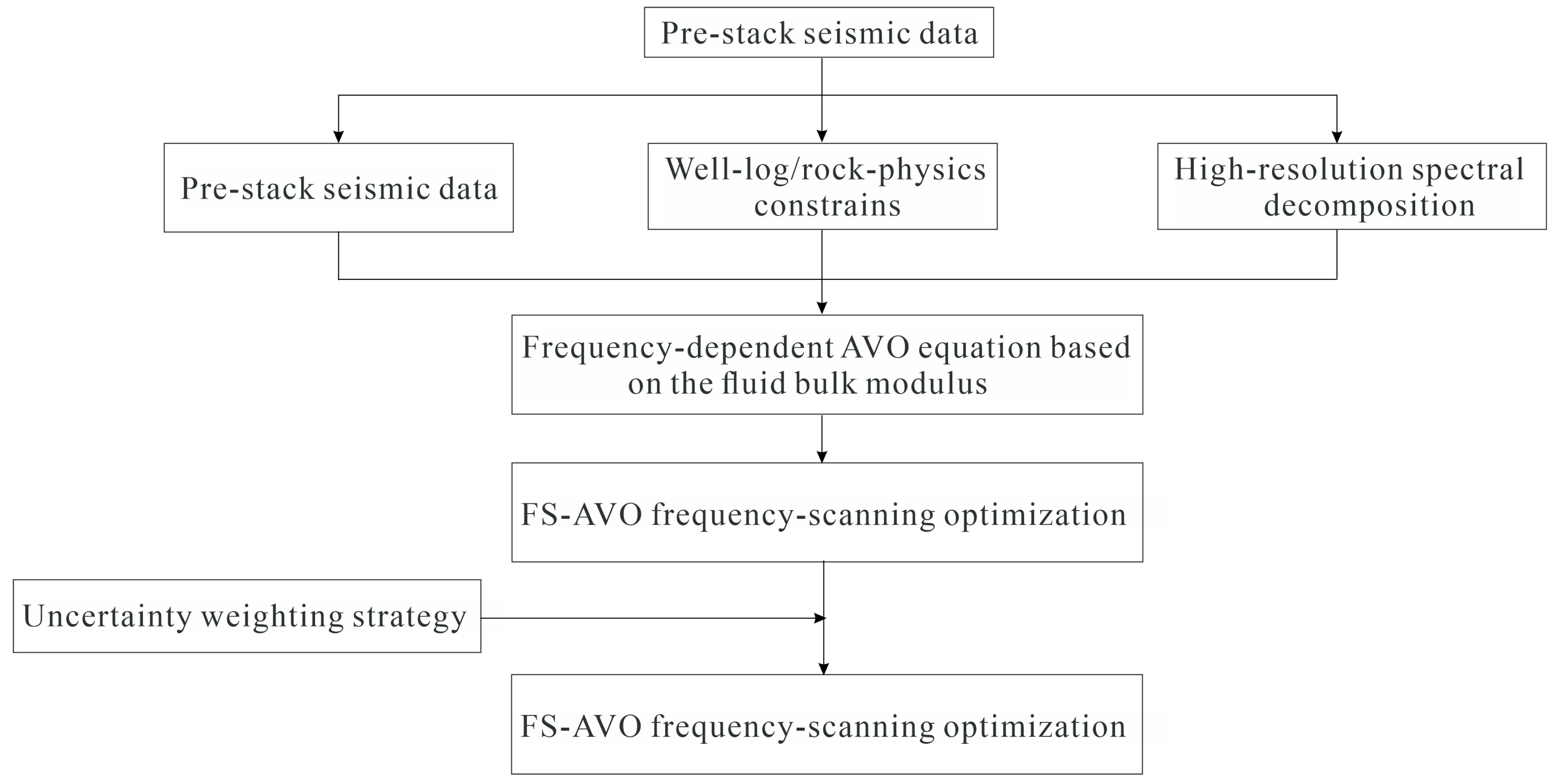
The implementation workflow is summarized as follows (Figure 3). First, prestack seismic gathers are divided into near-, mid-, and far-angle stacks or processed directly as angle gathers according to data quality. Second, a statistical wavelet is extracted from the seismic data, and the wavelet spectrum is used to determine the reliable frequency band. Third, MP-WVD spectral decomposition is applied to each angle stack to obtain local time–frequency spectra. Fourth, local frequency-scanning AVO inversion is performed within moving narrow frequency windows. Fifth, local inversion uncertainty and frequency-domain consistency are calculated for each time sample. Finally, multi-window estimates are fused to obtain the URFS-AVO fluid-dispersion attribute and compared with well-log interpretation.

4. Theoretical Tests and Robustness Analysis

4.1. Rock-Physics Model and Parameter Setup

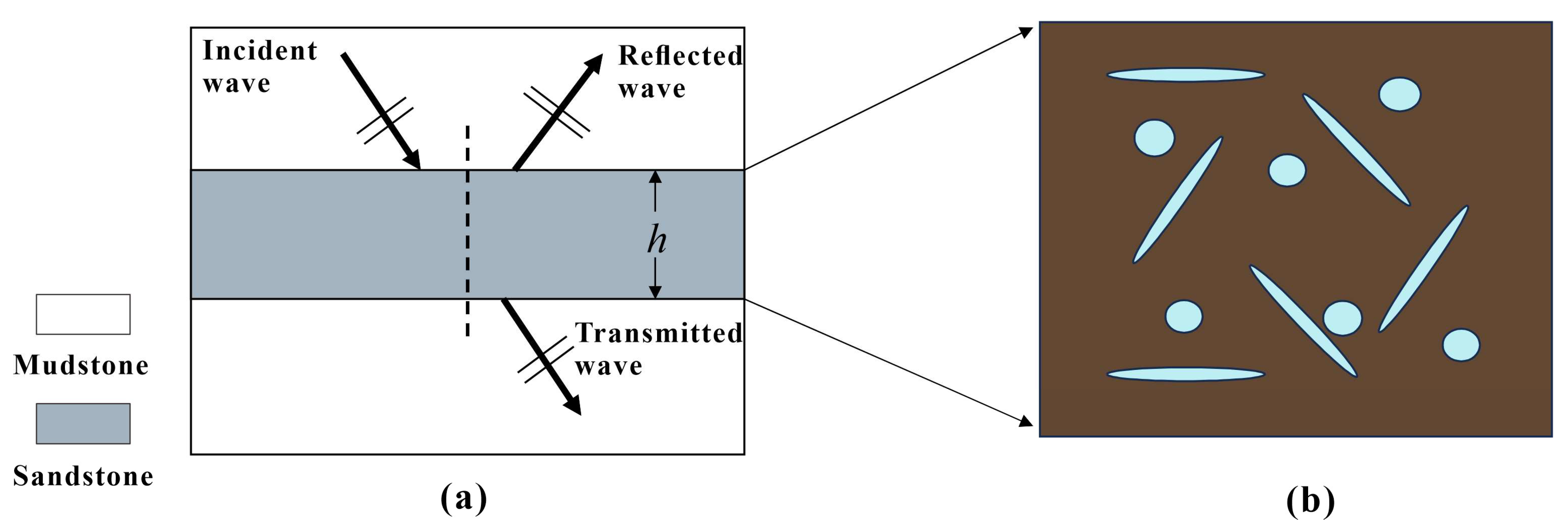
The theoretical tests are designed to evaluate the fluid sensitivity and noise robustness of the proposed URFS-AVO workflow under controlled conditions. A three-layer model is constructed, in which the target sandstone layer is embedded between two isotropic mudstone layers (Figure 4a). The target layer is a 10 m-thick low-permeability gas-bearing sandstone. The P-wave velocity, S-wave velocity, and density of the mudstone are 4.0 km/s, 2.1 km/s, and 2.45 g/cm³, respectively. The reference P-wave velocity, S-wave velocity, and grain density of the sandstone are 4.25 km/s, 2.30 km/s, and 2.30 g/cm³, respectively. The gas saturation of the target layer is set to $S_g=0.2$, $S_g=0.5$, and $S_g=0.8$.

The target sandstone is represented using the Chapman pore–microcrack model, which describes frequency-dependent elastic properties caused by pressure relaxation between stiff pores and compliant microcracks [18]. The complex stiffness of the saturated rock can be expressed as a background stiffness minus perturbations caused by pores, microcracks, and mesoscopic fractures:

$$\begin{array}{c}{C}_{ijkl}(\omega )=C_{ijkl}^0-{\varphi }_p{C}_{ijkl}^1(\omega )-{\epsilon }_c{C}_{ijkl}^2(\omega )-{\epsilon }_f{C}_{ijkl}^3(\omega ).\end{array}$$

(35)

Here, $C_{ijkl}^0$ is the isotropic background stiffness, $C_{ijkl}^1$, $C_{ijkl}^2$, and $C_{ijkl}^3$ are the stiffness perturbations caused by stiff pores, microcracks, and mesoscopic fractures, respectively; ${\varphi }_p$ is stiff-pore porosity, ${\epsilon }_c$ is microcrack density, and ${\epsilon }_f$ is mesoscopic fracture density. This study focuses on pore–microcrack-scale local fluid flow in low-permeability sandstone and sets ${\epsilon }_f=0$. Equation (35) is therefore simplified as

$$\begin{array}{c}{C}_{ijkl}(\omega )=C_{ijkl}^0-{\varphi }_p{C}_{ijkl}^1(\omega )-{\epsilon }_c{C}_{ijkl}^2(\omega ).\end{array}$$

(36)

The main input parameters of the Chapman model are listed in

Table 2. Main input parameters of the Chapman pore–microcrack model.

Parameter	Symbol	Value	Unit
Reference P-wave velocity	$V_{P0}$	4.250	km/s
Reference S-wave velocity	$V_{S0}$	2.300	km/s
Grain density	${\rho }_s$	2.300	g/cm3
Stiff-pore porosity	${\varphi }_p$	0.080	-
Permeability	$\kappa$	0.030	mD
Microcrack density	${\epsilon }_c$	0.100	-
Mesoscopic fracture density	${\epsilon }_f$	0	-
Microcrack aspect ratio	${\alpha }_c$	$2.0\times {10}^{-4}$	-
Effective pore–crack connection scale	$a$	$2.0\times {10}^{-3}$	m
Grain scale	$\zeta$	$2.0\times {10}^{-4}$	m
Water velocity	$V_w$	1.710	km/s
Gas velocity	$V_g$	0.620	km/s
Water density	${\rho }_w$	1.000	g/cm3
Gas density	${\rho }_g$	0.065	g/cm3
Water viscosity	${\eta }_w$	$1.0\times {10}^{-3}$	Pa·s
Gas viscosity	${\eta }_g$	$2.0\times {10}^{-5}$	Pa·s

.

For each gas-saturation case, the gas–water mixture properties are calculated using a linear density average, the Wood equation for bulk modulus, and a geometric viscosity mixture:

$$\begin{array}{l}\begin{array}{l}{\rho }_f=S_g{\rho }_g+(1-S_g){\rho }_w,\\ {\displaystyle \frac{1}{K_f^W}}={\displaystyle \frac{S_g}{K_g}}+{\displaystyle \frac{1-S_g}{K_w}},\\ {\eta }_f={\eta }_g^{S_g}{\eta }_w^{1-S_g},\end{array}\hfill \end{array}$$

(37)

where $K_g={\rho }_g{V}_g^2$ and $K_w={\rho }_w{V}_w^2$ are the gas and water bulk moduli, respectively. The microscopic relaxation time is calculated as

$$\begin{array}{c}\tau ={\displaystyle \frac{4{\eta }_f{a}^3(1-{\nu }_0)}{9\kappa \zeta {\mu }_0}},\end{array}$$

(38)

where ${\nu }_0$ and ${\mu }_0$ are the Poisson’s ratio and shear modulus of the background frame, respectively. The frequency-dependent PP-wave reflection response of the three-layer model is then computed using the generalized propagator matrix method [38], which accounts for incidence angle, frequency, layer thickness, and complex elastic parameters.

4.2. Elastic Properties Under Different Gas Saturations

Based on the parameters in Table 2, the Chapman model is used to calculate the frequency-dependent elastic responses of low-permeability gas-bearing sandstone under different gas saturations. The saturated-rock bulk modulus is first obtained from the frequency-dependent P- and S-wave velocities:

$$\begin{array}{c}{K}_{\mathrm{sat}}(\omega )={\rho }_{\mathrm{sat}}\left[V_P^2(\omega )-{\displaystyle \frac{4}{3}}{V}_S^2(\omega )\right].\end{array}$$

(39)

To obtain the fluid-bulk-modulus-related response used for sensitivity comparison, the low-frequency value of $K_{\mathrm{sat}}$ and the Wood mixed-fluid modulus are used to constrain the equivalent dry-frame bulk modulus $K_d$. Keeping $K_d$ fixed over the analyzed frequency band, the frequency-dependent equivalent fluid bulk modulus is back-calculated from the Gassmann equation as

$$\begin{array}{c}{K}_f(\omega )={\displaystyle \frac{\varphi }{\frac{{\left(1-K_d/K_0\right)}^2}{K_{\mathrm{sat}}(\omega )-K_d}-\frac{1-\varphi }{K_0}+\frac{K_d}{K_0^2}}},\end{array}$$

(40)

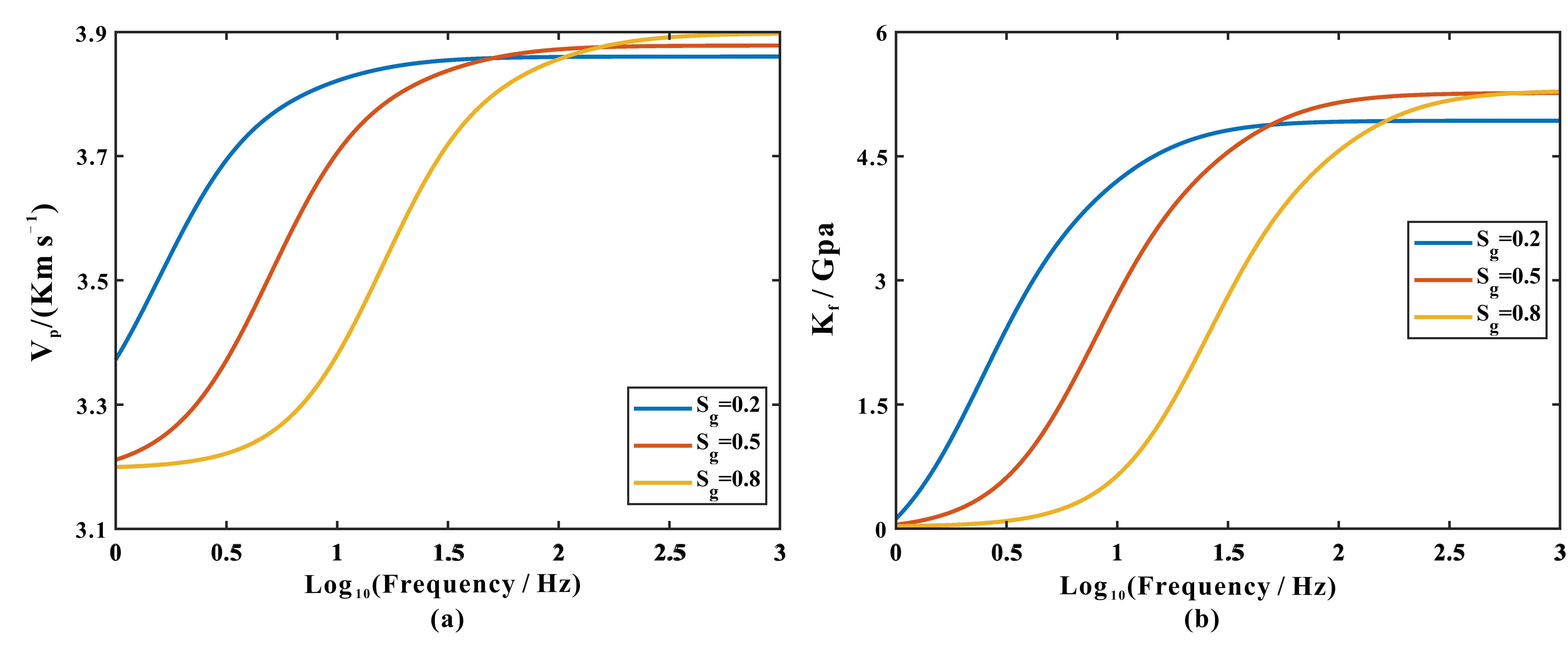
where $K_0$ is the mineral-grain bulk modulus. Figure 5 shows the frequency-dependent variations in P-wave velocity and $K_f$ for $S_g=0.2$, $S_g=0.5$, and $S_g=0.8$. As gas saturation increases, the P-wave velocity decreases and exhibits frequency-dependent variation (Figure 5). The $K_f$ curves exhibit a substantially larger amplitude variation with gas saturation than the $V_P$ curves, indicating that the fluid-bulk-modulus-related response is more sensitive to gas-saturation changes under the adopted model parameters.

4.3. Sensitivity of Interface Terms to Gas Saturation

FS-AVO inversion characterizes the frequency dependence of relative parameter perturbations across a reflection interface, rather than the absolute elastic properties of an individual layer. Therefore, the fluid sensitivity should be evaluated using the frequency-dependent relative contrasts between the upper mudstone and the target gas-bearing sandstone.

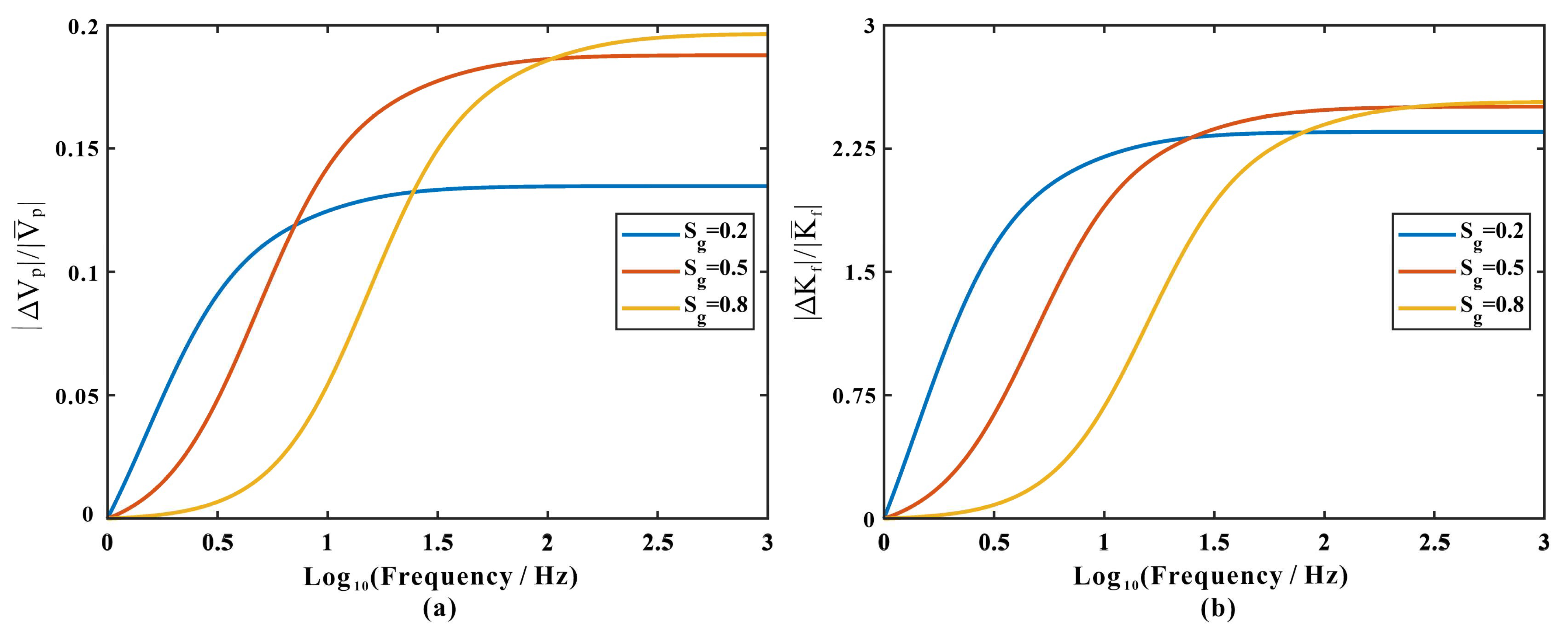
Figure 6 compares the frequency-dependent variations in these two interface terms for different gas saturations. The P-wave velocity-related interface perturbation varies relatively smoothly with frequency and shows only limited differences among the gas-saturation cases. In comparison, the fluid-bulk-modulus-related interface term exhibits a larger relative variation with frequency and a clearer separation among different gas saturations. This comparison indicates that the fluid-bulk-modulus-related interface perturbation is more sensitive to gas-saturation changes under the adopted rock-physics model and is therefore selected as the principal fluid-dispersion attribute in the subsequent FS-AVO and URFS-AVO inversion tests.

4.4. Frequency-Dependent PP-Wave Reflection Coefficient Spectra

On the basis of the interface sensitivity analysis, the generalized propagator matrix is used to calculate the frequency-dependent PP-wave reflection coefficient of the three-layer model. For each gas-saturation case, $R_{\mathrm{PP}}(\theta ,\omega )$ is calculated within 1–100 Hz and an incidence-angle range of 0–40 degrees. The corresponding band-limited reflection spectrum can be written as

$$\begin{array}{c}{S}_R(\theta ,\omega )=W_R(\omega )R_{\mathrm{PP}}(\theta ,\omega ),\end{array}$$

(41)

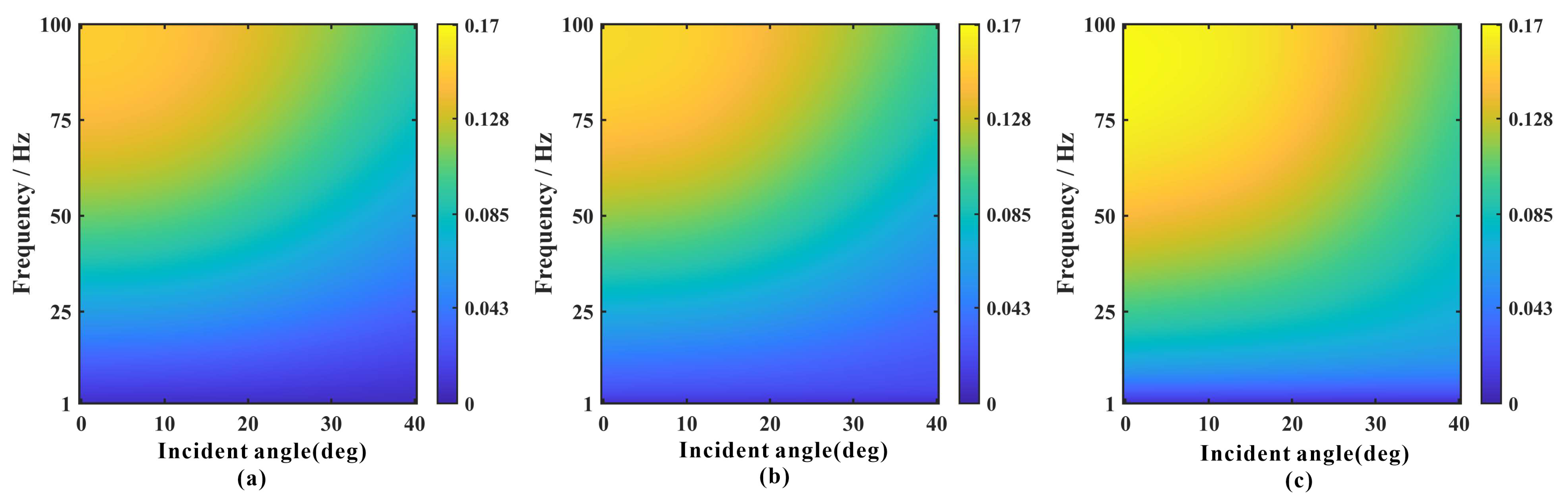
where $W_R(\omega )$ is the spectrum of the Ricker wavelet used in the synthetic forward modeling. Figure 7 shows that the PP-wave reflection spectra vary with both frequency and incident angle. With increasing gas saturation, the frequency-dependent reflection response of the target layer becomes more pronounced. This result confirms that the gas-related dispersion response can be expressed in the prestack frequency-angle domain, providing a physical basis for frequency-scanning AVO inversion.

4.5. Synthetic AVO Gathers and Time–Frequency Responses

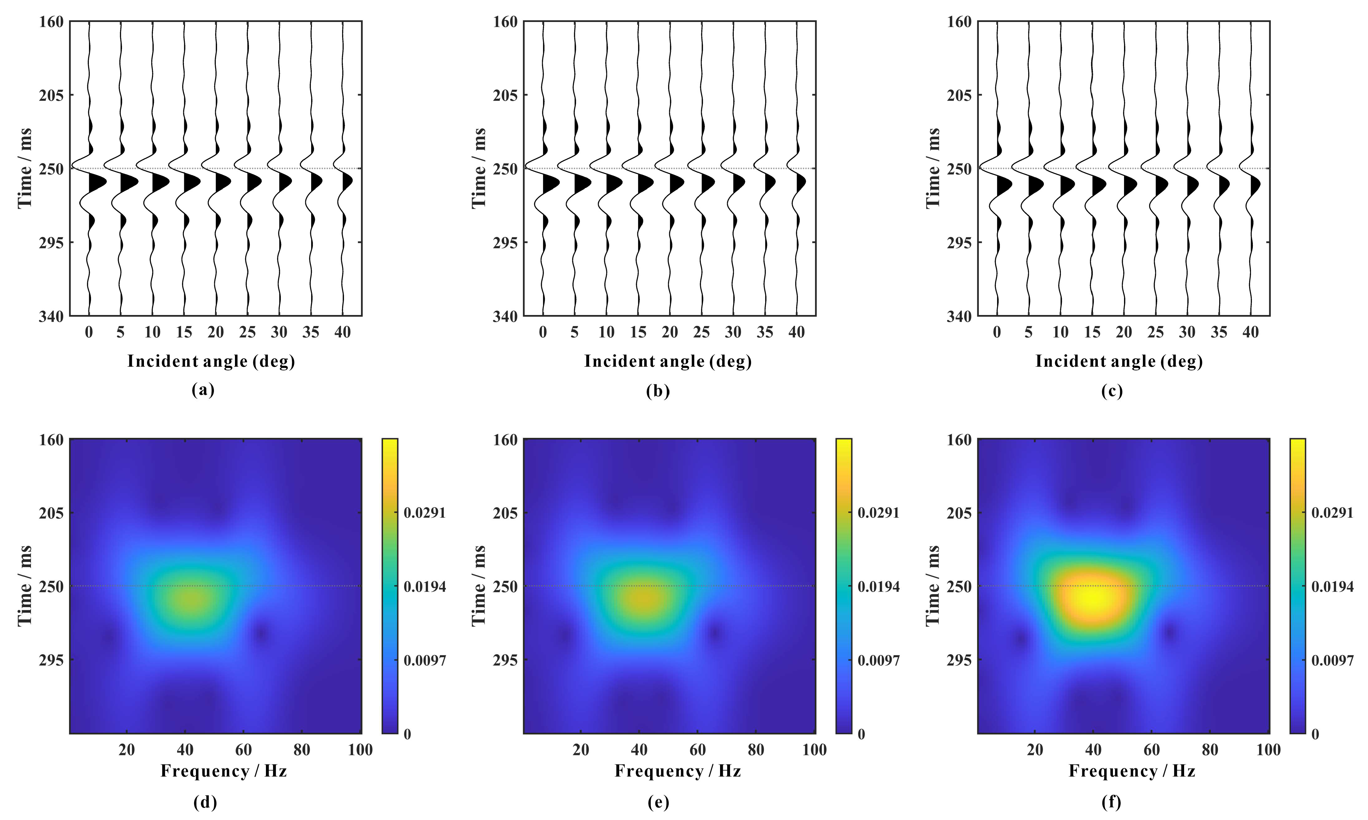
Synthetic prestack AVO gathers are generated using the modeled frequency-dependent reflection responses and a 35 Hz Ricker wavelet (Figure 8a–c). The target reflection event shows systematic amplitude variation with incident angle and gas saturation. The angle-stacked traces are then analyzed using MP-WVD spectral decomposition (Figure 8d–f). The time–frequency spectra show clear energy concentration near the target reflection event, and the local spectral response varies among the three gas-saturation cases. These tests indicate that the modeled gas-related frequency-dependent reflection behavior can be transferred to band-limited prestack seismic records and captured by local time–frequency analysis.

4.6. Noise-Free Inversion Test

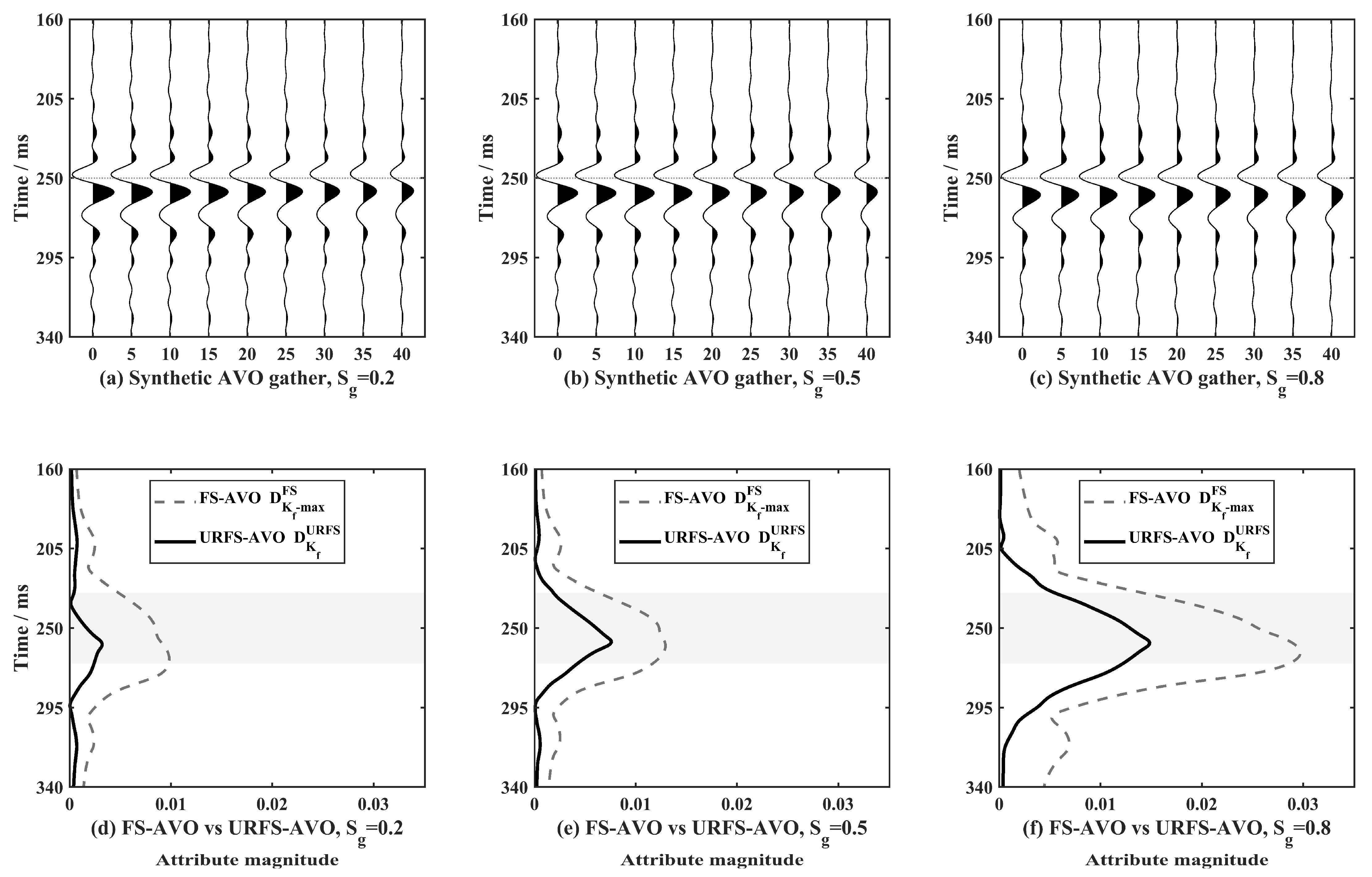
The maximum-window FS-AVO attribute and the proposed URFS-AVO attribute are calculated from the synthetic gathers without random noise (Figure 9). Both methods can identify the target gas-bearing layer. However, the maximum-window FS-AVO attribute tends to select the largest response among all local frequency windows and may produce broader or less stable background fluctuations. The URFS-AVO attribute uses inversion uncertainty and frequency-domain consistency to fuse the local estimates, resulting in a more concentrated anomaly near the target layer and weaker non-target responses. Within the approximately 230–270 ms target interval, the noise-free FS-AVO peak magnitudes are approximately 0.010, 0.013, and 0.030 for $S_g$ = 0.2, 0.5 and 0.8, respectively, whereas the corresponding URFS-AVO peak magnitudes are approximately 0.003, 0.008, and 0.015 (Figure 9).

In the implementation, the frequency-scanning inversion is carried out within the effective seismic frequency band. A series of scanning-center frequencies ${\omega }_c$ are selected at a constant interval, and a narrow moving frequency window is constructed around each center frequency. For each local window, the fluid-bulk-modulus-related dispersion attribute is estimated independently from the prestack angle gathers. In both the noise-free and noisy tests, the scanning-center frequencies range from 20 to 60 Hz at intervals of 5 Hz. Each moving frequency window has a half-width of 4 Hz, corresponding to a full window width of $h=8$ Hz in Equation (23). The uncertainty-weighting exponent in Equation (32) is set to $\alpha =0.2$ for all theoretical inversions.

The range of scanning-center frequencies, the moving-window bandwidth, and the uncertainty-weighting exponent $\alpha$ are the main parameters considered during parameter selection. Tests using different parameter combinations indicate that the scanning-center range determines the spectral information included in the inversion, whereas the moving-window bandwidth affects the balance between frequency localization and inversion stability. The exponent $\alpha$ controls the contrast among the uncertainty-based weights: a larger value emphasizes lower-uncertainty windows, whereas a smaller value produces more uniform contributions from the local estimates. Based on the effective seismic frequency band and the comparison of the inversion responses, the adopted parameters provide a suitable balance among target-response concentration, suppression of non-target fluctuations, and inversion stability.

4.7. Noisy Inversion Test

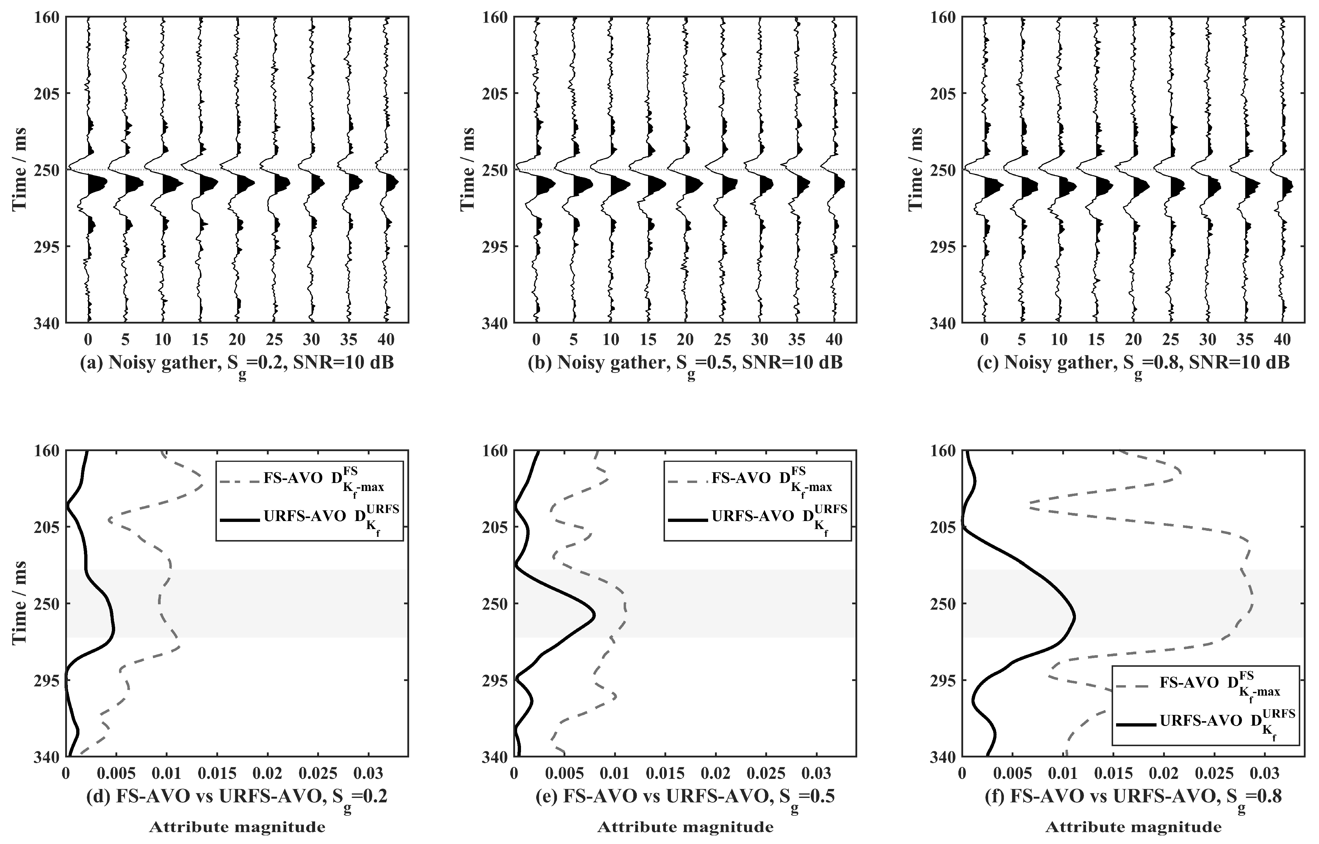
To evaluate noise robustness, Gaussian random noise (10 db) is added to the synthetic gathers, and the two inversion attributes are recalculated (Figure 10). Under noisy conditions, the maximum-window FS-AVO attribute is more easily affected by isolated anomalous frequency windows, which can lead to enhanced background fluctuations and unstable peak positions. By contrast, the URFS-AVO attribute maintains a clearer target-layer response because unreliable frequency windows receive lower weights and polarity-inconsistent local estimates are suppressed by the frequency-domain consistency coefficient. Within the same target interval, the peak magnitudes in the representative 10 dB noisy realization are approximately 0.012, 0.012, and 0.030 for FS-AVO and 0.005, 0.009, and 0.012 for URFS-AVO at $S_g$ = 0.2, 0.5, and 0.8, respectively (Figure 10). Although the fused URFS-AVO magnitudes are lower than the maximum-window values, their dominant responses remain concentrated within the target interval and exhibit weaker out-of-target fluctuations.

This comparison demonstrates that the proposed fusion strategy improves the stability of frequency-scanning AVO inversion under noisy conditions. From a computational perspective, the principal workload of the workflow arises from the time–frequency spectral calculation and the repeated local FS-AVO inversions over the scanning windows. The local frequency-window estimates are shared by maximum-window FS-AVO and URFS-AVO. URFS-AVO subsequently performs uncertainty-weight normalization, cross-window polarity-consistency evaluation, and weighted fusion. These additional operations increase approximately linearly with the number of scanning windows and do not require another set of local inversions.

5. Field Application

5.1. Seismic Data and Prestack Angle Profiles

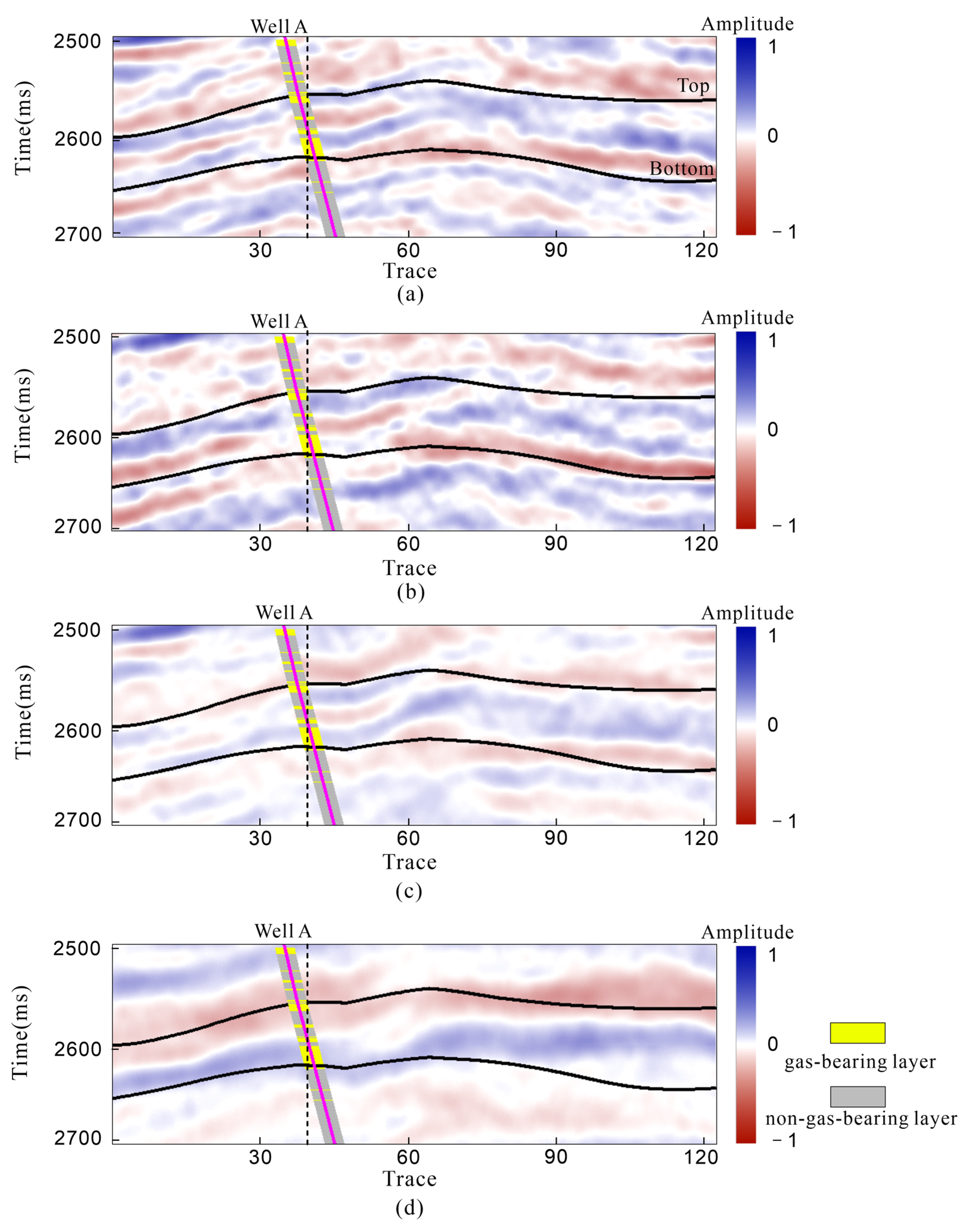
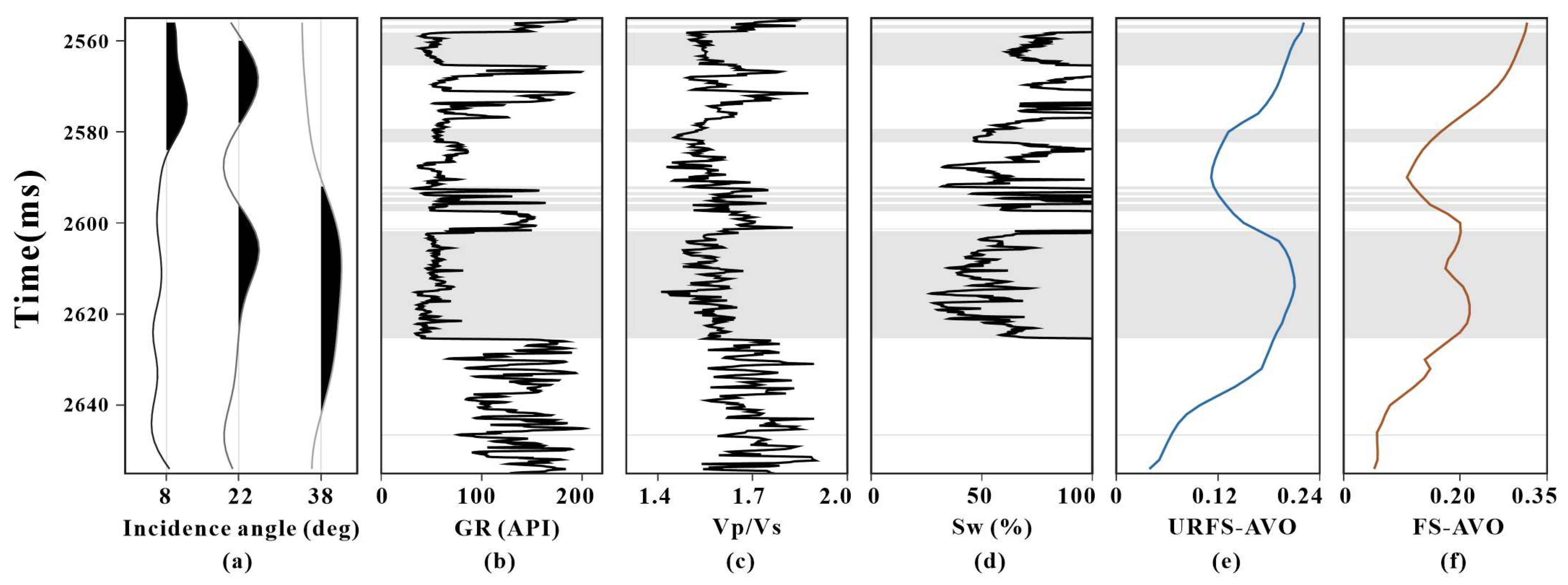
The proposed uncertainty-weighted robust frequency-scanning AVO (URFS-AVO) method was applied to marine prestack seismic data from the W area in the Xihu Sag, East China Sea. The target interval is the gas-bearing sandstone reservoir of the Huagang Formation. The available seismic data include post-stack seismic data and prestack angle-stack data. To examine the amplitude behavior around the target interval and to evaluate the quality of the prestack data, the post-stack profile and three representative prestack angle-stack profiles were compared (Figure 11). The selected central angles are approximately 8°, 22°, and 38°, corresponding to the small-angle, middle-angle, and large-angle stacks, respectively. For the field implementation, the URFS-AVO attribute was calculated exclusively from the seismic data and seismic-derived auxiliary information, including the background $V_P/V_S$ ratio obtained from seismic inversion. The Well A logs and interpreted gas-bearing interval were withheld from the inversion and attribute construction and were used only afterward for independent blind-well evaluation.

Because Well A is a deviated well, its trajectory cannot be represented by a single vertical seismic trace throughout the target interval. For the well-side comparison in this study, a representative seismic gather located near the middle part of the deviated well trajectory was selected, as indicated by the black dashed line in Figure 11. The seismic attribute curve used in the subsequent single-trace comparison was extracted from this selected gather, whereas the well-log curves were plotted along the actual deviated well path. This treatment provides a practical reference for comparing the seismic attribute response with the interpreted gas-bearing interval without forcing the deviated well trajectory onto a single vertical trace.

5.2. Time–Frequency Analysis and Wavelet Extraction

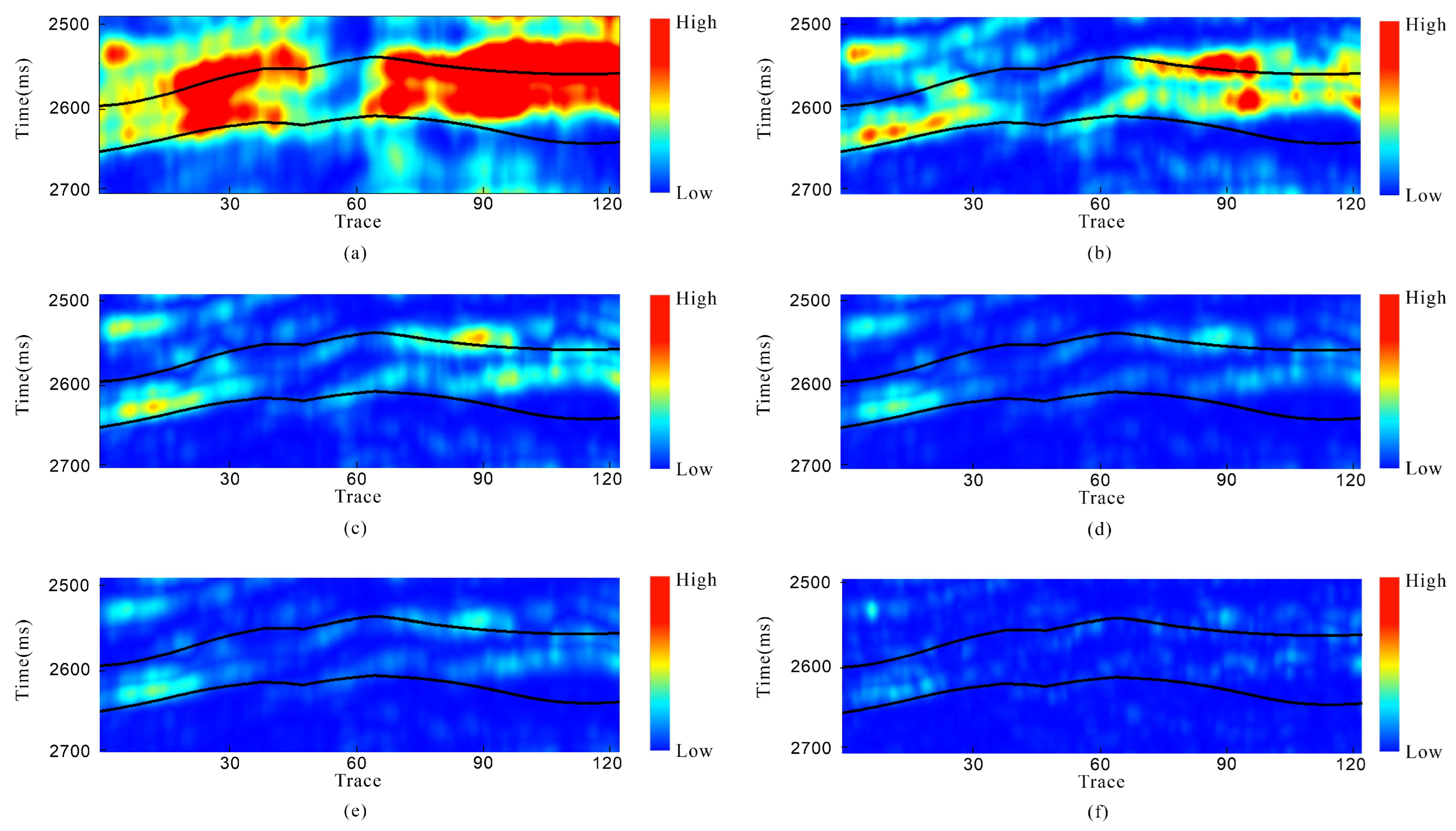
The large-angle seismic data were selected for time–frequency analysis. At the same time, far-angle data are usually more affected by limited bandwidth and noise; therefore, the effective frequency range needs to be evaluated before frequency-scanning inversion. MP-WVD spectral decomposition was applied to obtain instantaneous frequency-energy sections at selected frequencies (Figure 12). The frequency sections at 10, 20, 25, 30, 40, and 50 Hz show the vertical and lateral distribution of spectral energy around the target interval. These results were used to identify the reliable frequency band and to guide the selection of moving frequency windows for URFS-AVO inversion.

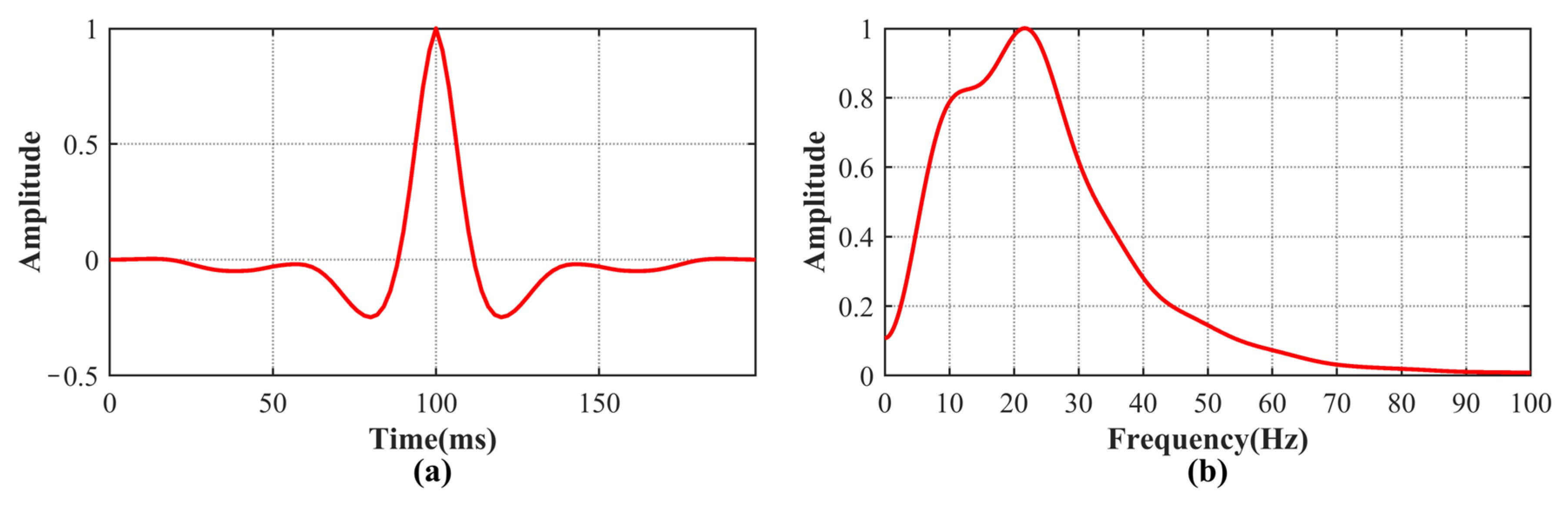
A statistical wavelet was extracted from the seismic data around the target interval (Figure 13). The extracted wavelet and its amplitude spectrum provide the spectral constraint required for the frequency-domain inversion. This step is important for marine prestack data because the frequency-scanning inversion should be conducted only within the reliable seismic bandwidth where both the seismic signal and wavelet spectrum remain stable.

Based on the extracted seismic wavelet spectrum and the time–frequency energy distribution of the prestack data, the reliable frequency band for field inversion is determined as 10–45 Hz. The scanning-center frequencies range from 10 to 45 Hz at intervals of 1 Hz. Each moving frequency window has a half-width of 5 Hz, corresponding to a full window width of $h=10$ Hz in Equation (23). The uncertainty-weighting exponent in Equation (32) is set to $\alpha =0.2$, consistent with that used in the theoretical tests. The same moving-window frequency-scanning procedure as that used in the synthetic tests is adopted.

For each scanning window, local FS-AVO inversion is first performed to obtain the $K_f$-related dispersion estimate. The proposed URFS-AVO attribute is then calculated by fusing the multi-window estimates using the local inversion uncertainty and frequency-domain consistency. For comparison, the conventional FS-AVO attribute is obtained by extracting the maximum response among all scanning windows.

5.3. Well-Side Single-Trace Comparison

Figure 14 compares the selected seismic trace, well-log interpretation, and inversion-attribute curves at Well A. The seismic trace used for this comparison corresponds to the representative gather marked by the black dashed line in Figure 11. The well-log curves, including the interpreted gas-bearing interval, are displayed along the actual deviated well path. Because the Well A information was withheld from the inversion and attribute construction, Figure 14 provides an independent blind-well evaluation of the seismic prediction. Owing to the deviated well trajectory, however, the comparison is made between a representative seismic gather close to the well trajectory and the reservoir interval along the actual well path and should not be interpreted as a strict trace-by-trace match along the entire trajectory.

The URFS-AVO curve shows enhanced responses around the interpreted gas-bearing interval. In comparison, the maximum-window FS-AVO curve exhibits broader and more fluctuating responses. This difference is consistent with the theoretical tests: FS-AVO extracts the largest response among all scanning windows, whereas URFS-AVO emphasizes responses that are supported by reliable and frequency-consistent windows. The well-side comparison therefore indicates that the uncertainty-weighted fusion strategy can reduce the influence of isolated anomalous frequency windows and improve the interpretability of the fluid-dispersion attribute.

5.4. Profile-Scale Comparison Between URFS-AVO and FS-AVO

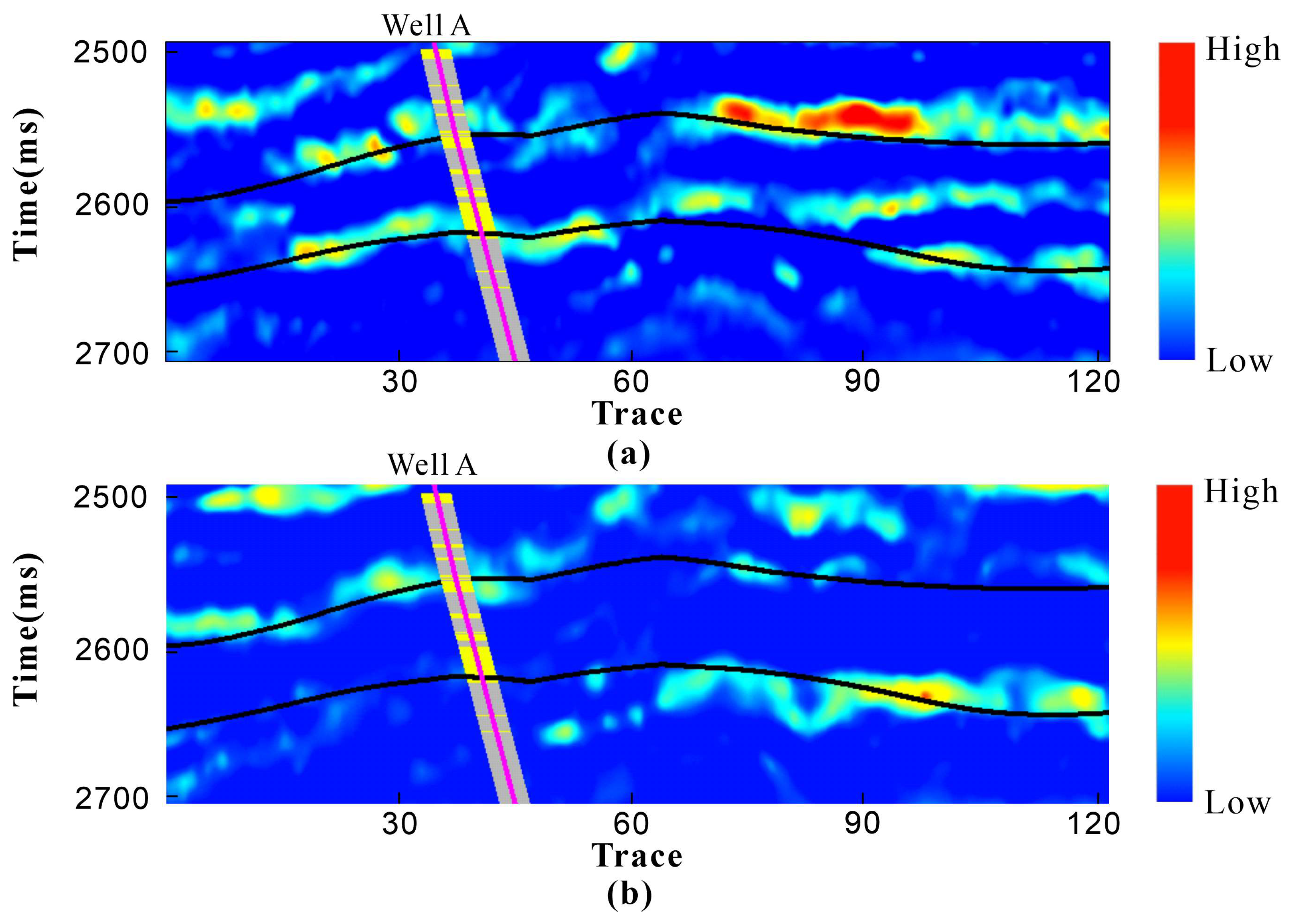
The URFS-AVO and maximum-window FS-AVO attributes were further compared on the seismic profile crossing Well A (Figure 15). Both attributes were obtained from the same prestack angle data, the same time–frequency spectra, and the same frequency-scanning windows; therefore, the difference between the two profiles mainly reflects the effect of the multi-window fusion strategy. The URFS-AVO result shows a more focused high-value anomaly near the target gas-bearing interval, while the background response outside the target zone is relatively weak and laterally more stable. In contrast, the FS-AVO result contains stronger local fluctuations away from the target interval, which may be associated with isolated frequency-window responses, uneven spectral energy, or thin-bed tuning.

The profile-scale comparison demonstrates the practical value of URFS-AVO for marine low-permeability sandstone prediction. The method does not simply retain the maximum local dispersion response; instead, it evaluates the reliability of each frequency-window estimate through local inversion uncertainty and frequency-domain consistency. As a result, the final attribute is less dominated by a single anomalous window and is better suited for identifying stable gas-related seismic responses in bandwidth-limited marine prestack data.

6. Discussion

6.1. Role of Uncertainty-Weighted Fusion in Frequency-Scanning AVO

The key methodological distinction between maximum-window FS-AVO and URFS-AVO lies in the treatment of the local frequency-window estimates. Frequency scanning is useful because it avoids relying on a single fixed reference frequency and allows the inversion to follow the local frequency-dependent response within the effective seismic band. However, when the final attribute is defined only by the maximum absolute value among all scanning windows, the result may be strongly controlled by a single local window. This behavior is beneficial for highlighting strong local anomalies, but it may also amplify responses caused by weak spectral energy, local noise, or an ill-conditioned inversion matrix.

URFS-AVO modifies the way in which the local frequency-window estimates are combined. In practical terms, maximum-window FS-AVO identifies the window with the largest absolute response, whereas URFS-AVO evaluates both the estimated reliability of each window and the polarity agreement among windows before fusion. A high-uncertainty estimate receives a smaller weight, while mutually opposing signed estimates reduce the cross-window polarity-consistency factor. The final attribute is therefore less sensitive to a high-uncertainty or polarity-conflicting window. This formulation does not impose general spectral smoothness; rather, it provides reliability- and polarity-aware fusion of the local inversion estimates.

This distinction is important for marine low-permeability sandstone reservoirs. The target layers are laterally heterogeneous, and the usable prestack bandwidth may vary with time, offset, and local signal-to-noise ratio. Under these conditions, a robust fusion strategy is more appropriate than a pure maximum-window operator. The theoretical and field results in this study both show that URFS-AVO can preserve the target-layer fluid-related response while reducing background fluctuations.

6.2. Geological and Seismic Implications of the Field Results

The W area in the Xihu Sag is characterized by low-permeability gas-bearing sandstone reservoirs in the Huagang Formation. The reservoir response is controlled by depositional facies, pore-structure heterogeneity, and gas saturation. These factors jointly affect the seismic amplitude, frequency content, and AVO behavior. Conventional post-stack amplitude or single elastic attributes may therefore be insufficient for stable fluid prediction. The URFS-AVO attribute uses both angle-dependent amplitude information and local frequency-dependent spectral differences, which provide an additional constraint for gas-bearing sandstone identification.

In the field application, the high-value URFS-AVO anomaly is spatially associated with the interpreted gas-bearing interval near Well A. Compared with FS-AVO, the URFS-AVO profile is less affected by scattered non-target anomalies and shows a more focused response around the reservoir interval. This observation is consistent with the theoretical tests, where uncertainty-weighted fusion suppresses unstable scanning windows under both noise-free and noisy conditions. The field result therefore supports the interpretation that URFS-AVO is more suitable for extracting stable gas-related dispersion anomalies from marine prestack seismic data.

6.3. Limitations and Future Work

Several practical limitations of the present study should be acknowledged. First, the inversion quality depends on the reliability of the time–frequency spectra, the estimated wavelet, the available prestack angle information, and the selected frequency band and window half-width. Consequently, the method may face challenges when the usable seismic bandwidth is narrow or uneven, far-angle spectral energy is weak, the prestack signal-to-noise ratio is low, wavelet estimation is unstable, or thin-bed tuning is strong. Under these conditions, uncertainty-weighted fusion can reduce the influence of isolated unstable frequency windows but cannot recover frequency or angle information that is absent from the input data. Second, the frequency band, window half-width, and uncertainty-weighting exponent $\alpha$ are currently selected according to the seismic bandwidth and data quality rather than through a fully adaptive procedure. Third, although Well A provides an independent blind-well evaluation because its logging data and interpreted gas-bearing interval were not used in the inversion or attribute construction, the field assessment is limited to one marine study area and one deviated well and therefore does not constitute multiwell validation. Future work will focus on adaptive frequency-window and weighting-parameter selection, improved treatment of noise and uneven spectral energy, and validation using additional wells and datasets.

7. Conclusions

This study proposes an uncertainty-weighted robust frequency-scanning AVO inversion method for marine gas-bearing sandstone identification. The method combines a fluid-bulk-modulus-related frequency-dependent AVO equation, high-resolution time–frequency analysis, local frequency-scanning inversion, and uncertainty-weighted multi-window fusion. Based on rock-physics modeling, synthetic prestack seismic tests, and field marine seismic application in the W area of the Xihu Sag, the main conclusions are as follows:

(1)

Rock-physics modeling based on the Chapman pore–microcrack model shows that the elastic response of low-permeability gas-bearing sandstone varies systematically with gas saturation. Compared with the P-wave velocity response, the fluid-bulk-modulus-related term exhibits a stronger sensitivity to gas-saturation variations under the tested model parameters. Frequency-dependent PP-wave reflection spectra further demonstrate that gas-related dispersion effects can be transferred to prestack seismic reflection responses and provide a physical basis for frequency-dependent AVO inversion.

(2)

Synthetic inversion tests show that the proposed URFS-AVO method provides a more stable fluid-dispersion attribute than the conventional FS-AVO maximum-window attribute. In the noise-free case, URFS-AVO preserves the target-layer anomaly while reducing background fluctuations. Under 10 dB Gaussian random noise, the uncertainty-weighted fusion suppresses isolated anomalous frequency windows and improves the continuity and localization of the target-layer response. These results indicate that the proposed fusion strategy does not simply enhance the maximum amplitude but emphasizes frequency windows with higher inversion reliability and better frequency-domain consistency.

(3)

Field application to marine prestack seismic data from the W area of the Xihu Sag shows that the URFS-AVO attribute delineates gas-bearing sandstone intervals more clearly than the FS-AVO maximum-window result. The high-value anomalies are generally consistent with the interpreted gas-bearing interval of Well A, and the profile-scale distribution agrees with the expected response of low-permeability gas-bearing sandstone in the Huagang Formation. The proposed method therefore provides a useful seismic constraint for fluid prediction in thinly interbedded marine low-permeability sandstone reservoirs.

References

1. Chang, Y.; Jiao, S.; Liu, Y.; Li, X.; Xiong, Z.; Chang, W.; Wang, J. Genesis and exploration significance of sweet-spot reservoirs in the Huagang Formation of the Q Structure, Central Anticlinal Belt, Xihu Sag. China Offshore Oil Gas 2026, 38, 48–59. [Google Scholar]
2. Liang, Z.; Jiang, Z.; Wu, W.; Guo, J.; Wang, M.; Nie, Z.; Li, Z.; Xu, D.; Xue, Z.; Chen, R.; et al. Study and Classification of Porosity Stress Sensitivity in Shale Gas Reservoirs Based on Experiments and Optimized Support Vector Machine Algorithm for the Silurian Longmaxi Shale in the Southern Sichuan Basin, China. ACS Omega 2022, 7, 33167–33185. [Google Scholar] [CrossRef] [Scilit] [PubMed]
3. Liang, Z.; Jiang, Z.; Han, Y.; Wang, B.; Wu, W.; Li, Z.; Li, Y.; Xue, Z. A Modified Dent-Fractal Mathematical Model to Investigate the Water Vapor Adsorption on Nanopore Structure Heterogeneity from the Longmaxi Shale, Sichuan Basin, China. Energy Fuels 2023, 37, 9131–9150. [Google Scholar] [CrossRef] [Scilit]
4. Li, P.; Gong, H.; Jiang, Z.; Zhang, F.; Liang, Z.; Wang, Z.; Wu, Y.; Shao, X. Characteristics and Influencing Factors of Multi-Scale Pore Structure Heterogeneity of Lacustrine Shale in the Gaoyou Sag, Eastern China. Minerals 2023, 13, 359. [Google Scholar] [CrossRef] [Scilit]
5. Meng, M.; Li, Z.; Hong, Z.; Bao, J.; Jiang, Q. Quantifying Pore Size Distribution by Nuclear Magnetic Resonance Method in Tight Sandstones: Comparison between Water-Wet and Oil-Wet Saturated Fluids. Int. J. Hydrogen Energy 2026, 197, 152608. [Google Scholar] [CrossRef] [Scilit]
6. Hong, Z.; Meng, M.; Yuan, B.; Ma, C.; Wang, Q.; Deng, K.; Bao, J.; Yuan, M. Nanopore Structure Characterization of Lacustrine and Marine Shales: Comparison between Small Angle Neutron Scattering and Nitrogen Adsorption Methods. Int. J. Hydrogen Energy 2026, 208, 153565. [Google Scholar] [CrossRef] [Scilit]
7. Bao, J.; Meng, M.; Wang, Q.; Yu, S.; Yuan, M.; Hong, Z.; Jiang, Q. Comparison of Square-Root and Logarithmic Data Treatment for Pore Connectivity by Co-Current Spontaneous Imbibition in Lacustrine Shales. Int. J. Hydrogen Energy 2026, 229, 154737. [Google Scholar] [CrossRef] [Scilit]
8. Aki, K.; Richards, P. Quantitative Seismology: Theory and Methods; W H Freeman & Co.: San Francisco, CA, USA, 1980. [Google Scholar]
9. Gray, D. Elastic Inversion for Lamé Parameters. Seg. Tech. Program Expand. Abstr. 2002, 21, 213–216. [Google Scholar]
10. Smith, G.C.; Gidlow, P.M. Weighted stacking for rock property estimation and detection of gas. Geophys. Prospect. 1987, 35, 993–1014. [Google Scholar] [CrossRef] [Scilit]
11. Goodway, W.; Chen, T.; Downton, J. Improved AVO Fluid Detection and Lithology Discrimination Using Lamé Parameters; “λρ”,“μρ”,&“λ/μ fluid stack”, from P and S inversions. In 67th Annual International Meeting, 2–7 November 1997; SEG: Houston, TX, USA; pp. 183–186. [CrossRef] [Scilit]
12. Russell, B.H.; Hedlin, K.; Hilterman, F.J.; Lines, L.R. Fluid-Property Discrimination with AVO: A Biot-Gassmann Perspective. Geophysics 2003, 68, 29–39. [Google Scholar] [CrossRef] [Scilit]
13. Russell, B.H.; Gray, D.; Hampson, D.P. Linearized AVO and Poroelasticity. Geophysics 2011, 76, C19–C29. [Google Scholar] [CrossRef] [Scilit]
14. Zong, Z.; Yin, X.; Wu, G. Direct Inversion for a Fluid Factor and Its Application in Heterogeneous Reservoirs. Geophys. Prospect. 2013, 61, 998–1005. [Google Scholar] [CrossRef] [Scilit]
15. Yin, X.; Zhang, S. Bayesian Inversion for Effective Pore-Fluid Bulk Modulus Based on Fluid-Matrix Decoupled Amplitude Variation with Offset Approximation. Geophysics 2014, 79, R221–R232. [Google Scholar] [CrossRef] [Scilit]
16. Biot, M.A. Mechanics of Deformation and Acoustic Propagation in Porous Media. J. Appl. Phys. 1962, 33, 1482–1498. [Google Scholar] [CrossRef] [Scilit]
17. Ba, J.; Carcione, J.M.; Nie, J.X. Biot-Rayleigh Theory of Wave Propagation in Double-Porosity Media. J. Geophys. Res. 2011, 116, B06202. [Google Scholar] [CrossRef] [Scilit]
18. Chapman, M. Frequency-dependent Anisotropy Due to Meso-scale Fractures in the Presence of Equant Porosity. Geophys. Prospect. 2003, 51, 369–379. [Google Scholar] [CrossRef] [Scilit]
19. Gurevich, B.; Brajanovski, M.; Galvin, R.J.; Müller, T.M.; Toms-Stewart, J. P-wave Dispersion and Attenuation in Fractured and Porous Reservoirs—Poroelasticity Approach. Geophys. Prospect. 2009, 57, 225–237. [Google Scholar] [CrossRef] [Scilit]
20. Wang, P.; Cui, Y.; Li, J.; Liu, J. Theoretical Model for the Elastic Properties of Cracked Fluid-Saturated Rocks Considering the Crack Connectivity. Geophys. J. Int. 2024, 239, 1203–1216. [Google Scholar] [CrossRef] [Scilit]
21. Wilson, A.; Chapman, M.; Li, X.-Y.; Survey, B.G. Frequency-Dependent AVO Inversion. In 79th Annual International Meeting, 25–30 October 2009; SEG: Houston, TX, USA. [CrossRef] [Scilit]
22. Zhang, S.; Yin, X.; Zhang, G. Dispersion-Dependent Attribute and Application in Hydrocarbon Detection. J. Geophys. Eng. 2011, 498. [Google Scholar] [CrossRef] [Scilit]
23. Luo, X.; Chen, X.; Lv, B.; Liu, J.; Wu, H.; Wang, P. Frequency-Dependent AVO Inversion Using a Modified Window-Parameter-Optimized S-Transform for High Gas-Saturation Reservoir Delineation. IEEE Geosci. Remote Sens. Lett. 2023, 20, 3000805. [Google Scholar] [CrossRef] [Scilit]
24. Miao, F.; He, Y.; Wang, S.; Huang, H. A Novel Fluid Identification Method Based on a High-Precision Spectral Decomposition Method. J. Geophys. Eng. 2024, 21, 534–547. [Google Scholar] [CrossRef] [Scilit]
25. Guo, Z.-Q.; Zhang, T.; Liu, C. Direct Hydrocarbon Identification in Shale Oil Reservoirs Using Fluid Dispersion Attribute Based on an Extended Frequency-Dependent Seismic Inversion Scheme. Pet. Sci. 2023, 20, 1532–1545. [Google Scholar] [CrossRef] [Scilit]
26. Feng, Y.; Zong, Z.; Zhang, G.; Lang, K.; Chen, F. PP-Wave Reflection Coefficient Equation for HTI Media Incorporating Squirt Flow Effect and Frequency-Dependent Azimuthal AVO Inversion for Anisotropic Fluid Indicator. IEEE Trans. Geosci. Remote Sens. 2024, 62, 5906212. [Google Scholar] [CrossRef] [Scilit]
27. Lan, T.; Zong, Z.; Jia, W. Reservoir Hydrocarbon Identification Method Based on Prestack Seismic Frequency-Dependent Anisotropic Inversion. IEEE Trans. Geosci. Remote Sens. 2023, 61, 1–13. [Google Scholar] [CrossRef] [Scilit]
28. Li, Y.; Guo, Z.; Liu, C. Characterization of Fluid-Saturated Fractures Based on Seismic Azimuthal Anisotropy Dispersion Inversion Method. IEEE Trans. Geosci. Remote Sens. 2024, 62, 5915413. [Google Scholar] [CrossRef] [Scilit]
29. Junhwan, C.; Seokmin, O.; Joongmoo, B. Uncertainty Estimation in AVO Inversion Using Bayesian Dropout Based Deep Learning. J. Pet. Sci. Eng. 2022, 208, 109288. [Google Scholar] [CrossRef] [Scilit]
30. Perez-Roa, R.; Infante, S.; Barragan, G.; Manzanilla, R. Bayesian Inference Based on Algorithms: MH, HMC, MALA and Lip-MALA for Prestack Seismic Inversion. Nonlin. Process. Geophys. 2026, 33, 173–195. [Google Scholar] [CrossRef] [Scilit]
31. Yu, X.; Li, S.; Cao, B.; Hou, G.; Wang, Y.; Huangfu, Z. Oligocene sequence framework and depositional response in the Xihu Depression, East China Sea Shelf Basin. Acta Sedimentol. Sin. 2017, 35, 299–314. [Google Scholar] [CrossRef]
32. Li, S.; Yu, X.; Steel, R.; Zhu, X.; Li, S.; Cao, B.; Hou, G. Change from Tide-influenced Deltas in a Regression-dominated Set of Sequences to Tide-dominated Estuaries in a Transgression-dominated Sequence Set, East China Sea Shelf Basin. Sedimentology 2018, 65, 2312–2338. [Google Scholar] [CrossRef] [Scilit]
33. Zheng, W.; Yin, G.; Sun, L.; Wei, S.; Wei, X.; Niu, B. Sedimentary Systems of the Oligocene Huagang Formation in the Central Anticline Zone of the Xihu Depression, East China Sea Shelf Basin. Energy Geosci. 2024, 5, 100150. [Google Scholar] [CrossRef] [Scilit]
34. Han, D.; Batzle, M.L. Gassmann’s Equation and Fluid-Saturation Effects on Seismic Velocities. Geophysics 2004, 69, 398–405. [Google Scholar] [CrossRef] [Scilit]
35. Nur, A.; Mavko, G.; Dvorkin, J.; Galmudi, D. Critical Porosity: A Key to Relating Physical Properties to Porosity in Rocks. Lead. Edge 1998, 17, 357–362. [Google Scholar] [CrossRef] [Scilit]
36. Mallat, S.G.; Zhang, Z. Matching Pursuits with Time-Frequency Dictionaries. IEEE Trans. Signal Process. 1993, 41, 3397–3415. [Google Scholar] [CrossRef] [Scilit]
37. Cohen, L. Time-Frequency Distributions-a Review. Proc. IEEE 1989, 77, 941–981. [Google Scholar] [CrossRef] [Scilit] [PubMed]
38. Carcione, J.M. AVO Effects of a Hydrocarbon Source-Rock Layer. Geophysics 2001, 66, 419–427. [Google Scholar] [CrossRef] [Scilit]
Figure 1. Tectonic setting of the Xihu Sag, showing the W area and Well A within the Central Anticlinal Belt. The legend identifies the anticlinal structures, compressional and uplifted domains, structural-zonation and tectonic-unit boundaries, major faults, and well location.
Jmse 14 01566 g001
Figure 2. Schematic comparison of the fixed and moving frequency-window strategies used in frequency-scanning AVO inversion: (a) a fixed frequency window centred at one prescribed reference frequency (red dot), within which the P-wave velocity-frequency relation (blue curve) is represented by a single first-order linear approximation (red line); (b) a set of moving local frequency windows centred at multiple scanning frequencies (red dots), enabling the P-wave velocity-frequency relation to be characterized locally across the effective frequency band. Vertical dashed lines denote the boundaries of the frequency windows.
Jmse 14 01566 g002
Figure 3. Workflow of the proposed uncertainty-weighted robust frequency-scanning AVO (URFS-AVO) inversion method.
Jmse 14 01566 g003
Figure 4. Schematic diagrams of the layered reflection model and the Chapman pore-microcrack model: (a) a three-layer reflection model with a target sandstone layer (blue-grey; thickness h) embedded between two mudstone layers (white); the dashed vertical line denotes the normal to the horizontal interfaces, and the arrows indicate the incident, reflected, and transmitted waves; (b) a Chapman pore-microcrack model of the target sandstone, where the brown background represents the sandstone matrix, the light-blue rounded inclusions represent stiff pores, and the light-blue elongated inclusions represent compliant microcracks.
Jmse 14 01566 g004
Figure 5. Frequency-dependent elastic properties of the target sandstone for different gas saturations: (a) P-wave velocity, V p ; (b) equivalent fluid bulk modulus, K f . In both panels, the blue, orange, and yellow curves represent S g = 0.2, 0.5, and 0.8, respectively.
Jmse 14 01566 g005
Figure 6. Frequency-dependent relative interface terms for different gas-saturation cases: (a) relative P-wave-velocity term; (b) relative fluid-bulk-modulus-related term. In both panels, the curves correspond to S g = 0.2, 0.5, and 0.8, as indicated in the legend.
Jmse 14 01566 g006
Figure 7. Frequency-dependent PP-wave reflection coefficient spectra for different gas saturations: (a) S g = 0.2 ; (b) S g = 0.5 ; and (c) S g = 0.8 .
Jmse 14 01566 g007
Figure 8. Synthetic prestack AVO gathers and corresponding MP-WVD time–frequency spectra. (ac) are synthetic AVO gathers for different gas-saturation cases (0.2, 0.5, 0.8). (df) are time–frequency spectra of the corresponding stacked traces (0.2, 0.5, 0.8); (d) corresponds to the stacked trace of (a).The horizontal dashed line in all panels marks the reference time (250 ms) of the target reflection event.
Jmse 14 01566 g008
Figure 9. Noise-free theoretical inversion test comparing maximum-window FS-AVO and URFS-AVO attributes under different gas-saturation cases. Panels (ac) are synthetic AVO gathers for different gas-saturation cases (0.2, 0.5, 0.8). Panels (df) are theoretical inversion results of the corresponding prestack traces; panel (d) corresponds to the prestack trace of panel (a). The horizontal dashed line in panels (ac) marks the reference time (250 ms) of the target reflection event, whereas the grey shaded band in panels (df) denotes the target interval (approximately 230–270 ms).
Jmse 14 01566 g009
Figure 10. Theoretical inversion test with Gaussian random noise. Panels (ac) show synthetic AVO gathers for gas-saturation cases of 0.2, 0.5, and 0.8, respectively. Panels (df) show the theoretical inversion results obtained from the prestack traces in panels (ac), respectively. The horizontal dashed line in panels (ac) marks the reference time (250 ms) of the target reflection event, whereas the gray shaded band in panels (df) denotes the target interval (approximately 230–270 ms).
Jmse 14 01566 g010
Figure 11. Post-stack and prestack angle-stack seismic profiles through Well A. (a) is the post-stack seismic profile. (bd) are the small-angle, middle-angle, and large-angle profiles with central angles of approximately 8°, 22°, and 38°, respectively. The black dashed line marks the representative seismic gather selected for the well-side single-trace comparison. The magenta line marks the actual deviated trajectory of Well A, and the black dashed line marks the representative seismic gather selected for the well-side single-trace comparison.
Jmse 14 01566 g011
Figure 12. Instantaneous frequency-energy sections of the large-angle seismic data. Panels (af) correspond to 10, 20, 25, 30, 40, and 50 Hz, respectively. The two black lines delineate the upper and lower boundaries of the target layer.
Jmse 14 01566 g012
Figure 13. Extracted seismic wavelet and its amplitude spectrum. Panel (a) shows the time-domain wavelet, and panel (b) shows the corresponding amplitude spectrum.
Jmse 14 01566 g013
Figure 14. Well-side comparison between the selected seismic traces, well-log interpretation, and inversion attributes at Well A: (a) selected seismic traces at incidence angles of 8°, 22°, and 38°, respectively; (b) gamma-ray (GR) log; (c) P-wave-to-S-wave velocity ratio (Vp/Vs) log; (d) water saturation (Sw) log; (e) URFS-AVO attribute; and (f) maximum-window FS-AVO attribute. The black curves in panels (bd) represent the corresponding well logs, while the blue and brown curves in panels (e,f) represent the URFS-AVO and maximum-window FS-AVO attributes, respectively. The gray shaded bands in panels (bf) denote the interpreted gas-bearing intervals.
Jmse 14 01566 g014
Figure 15. Profile-scale comparison between the URFS-AVO and maximum-window FS-AVO attributes along the seismic profile crossing Well A: (a) URFS-AVO attribute; (b) maximum-window FS-AVO attribute. In both panels, the magenta line marks the actual deviated trajectory of Well A; the two black lines delineate the upper and lower boundaries of the target layer; and the yellow and gray shaded segments along the well trajectory denote gas-bearing and non-gas-bearing layers, respectively.
Jmse 14 01566 g015