Underwater Noise Monitoring at an Operational Nearshore Wind Farm: First Results from the SWIM Project

Abstract

Offshore wind energy is growing rapidly, as are concerns about the risks to marine species from underwater noise associated with it. The SWIM project aims to better understand and predict these impacts by monitoring an existing wind farm in the Gulf of Taranto (Italy). This work reports the first results obtained from analysing data acquired during the project’s surveys. Several natural and anthropogenic factors contribute to the Sound Pressure Level (SPL). We aim to identify and isolate them in order to understand the share and contribution due to wind turbine activity, and to test whether and how the wind regime can be considered a proxy for it. Components such as marine traffic and tides have been filtered using statistics and periodicities, while events associated with turbine activity have been identified through their correlation with the wind speed and the typical signature they leave in the spectrograms. Supported by preliminary evidence, the analysis suggests that noise can propagate up to 1400 m from the south-west-tip turbine of the wind farm, where wind speeds exceeding 10 m/s can increase the SPL by approximately 6 dB. Future work will model noise propagation and validate it with new recordings.

1. Introduction

Offshore wind power is rapidly becoming a very important source of energy, combining its clean, low-carbon, and sustainable nature with the availability of abundant, high-speed winds characteristic of offshore environments, resulting in significant potential for efficient power generation. According to the 2025 Global Wind Energy Council (GWEC) report [1], in 20 years, global wind capacity has grown more than twenty-fold, surpassing 1.1 TW or 8% of global electricity generation. In Italy, the focus area of our work, a Legambiente report [2] states that 93 new offshore wind farm projects are planned for Italian waters, with a combined capacity of approximately 75 MW.

Although positive environmental impacts from wind farms have been identified [3,4,5], and there is enthusiasm for the possibilities offered by offshore wind power, concerns have also emerged that this infrastructure could pose problems for the environment. These threats include, for example, the collision mortality of birds with turbines, displacement and habitat loss, impacts on migration, light attraction, and disorientation. A particular concern is also the potential impact on marine species due to underwater noise. Particularly, human-generated underwater noise was formally recognised as a major form of ocean pollution by the EU’s Marine Strategy Framework Directive (MSFD) [6] through its Descriptor 11. The MSFD suggests EU Member States keep energy inputs, including underwater noise, at levels that avoid harming the marine environment. In response, a range of monitoring programmes and biodiversity impact assessments have been coordinated by international bodies such as ACCOBAMS, HELCOM, and OSPAR, guided by specialist networks including EU TG Noise, HELCOM EN-Noise, and OSPAR ICG-Noise. At the same time, numerous European and international research programmes such as JOMOPANS, AGESCIC, quietMED, PI-AQUO, JONAS, QUIETSEAS, and SATURN have been initiated.

The Mediterranean Sea covers less than 1% of the world’s ocean surface, yet it stands as one of the most significant global biodiversity hotspots. It is also among the most threatened ecoregions, as human pressures on coastal and offshore ecosystems continue to endanger numerous species [7,8]. Anthropogenic underwater noise is increasingly recognised as a pervasive pollutant in marine ecosystems and as a stressor for several cetacean species [9]. The acoustic space that cetaceans rely on for vital biological functions—including communication with conspecifics, echolocation for prey detection and navigation, and orientation within both natural and social environments—may be significantly compromised [10,11,12,13]. Cetaceans may suffer physical and physiological harm, including permanent or temporary hearing threshold shifts [14] and acute or chronic neuroendocrine stress responses [15]. Beyond physiological effects, anthropogenic noise can drive significant behavioural alterations, including the avoidance of acoustically impacted areas [16]. For example, following [17], dolphins increase the frequency parameters of their whistles with lower variability in the presence of anthropogenic noise, and increase the end frequency of their whistles when confronted with increasing natural noise.

Despite meaningful advances in recent years, knowledge of noise pollution in seas and oceans remains limited, and several critical knowledge gaps have been identified. Scientific data on underwater sound environments remain scarce, and the technical challenges involved in monitoring, processing, and interpreting sound fields confirm that noise pollution is still inadequately understood and, consequently, inadequately regulated [18,19]. At the same time, not all possible noise sources have been analysed with equal attention. Most studies have concentrated on impulsive sources, pile driving, or marine traffic, while offshore wind farms have not yet been fully characterised. Modelling of underwater noise propagation is also problematic [20]. As a result, key physical phenomena may be neglected, leading to unreliable noise prediction and ineffective mitigation approaches.

Another current limitation in understanding underwater noise relates to the functional anatomy, physiology, and acoustic pathways of the hearing apparatus in marine mammals, which are also not well known. A deeper understanding of how sound is received and processed is essential before the specific impacts of underwater noise on these animals can be reliably modelled [21,22,23,24]. All these issues are further complicated by the difficulties in conducting viable direct experimental research on marine mammals, as it is very problematic to model and simulate animal responses to external acoustic stimuli or to predict the physiological and behavioural effects of known noise sources on these species.

Wind farm-related underwater noise can occur across all phases of the wind farm’s lifecycle, from construction and maintenance through operation and eventual decommissioning. These disturbances can pose potential risks to aquatic species and therefore raise questions about the expansion of this type of power generation. These considerations underpin the need to understand how noise is generated and how it travels in the designated area. According to [25] there are not many works in the scientific literature regarding the specific impact of wind farms. Most of these works focus on impulsive noise generated during the construction phase, while less is explored regarding the operational phase of offshore turbines.

Within this perspective, the SWIM project, funded by Next Generation EU PNRR-PRIN [26], aims to better characterise and predict the effects of offshore wind turbines on the marine soundscape, with particular attention to their operational phases, and to evaluate their potential impact on marine mammals. The project is carried out through three activities: (i) monitoring the soundscape and underwater noise related to an existing wind farm, (ii) modelling noise propagation in the designated area, and (iii) modelling wave propagation through the anatomy of cetaceans. This work has analysed observations and measurements taken during the monitoring phase of the SWIM project, while further investigation is planned on the other activities.

2. Materials and Methods

2.1. Location: The Gulf of Taranto

The SWIM project builds on the analysis of noise generated by existing wind farms to provide information on the potential impact of planned new sites. During the timeframe of the SWIM project, the unique active nearshore wind farm in the Mediterranean Sea is in the Gulf of Taranto (Northern Ionian Sea). The Beleolico infrastructure was launched in 2022 and comprises 10 MingYang Smart Energy MySE3.0-135 (Ming Yang, Ming Yang Industrial Park, No.22 HuoJu Road, Torch Development Zone, Zhongshan city, China) monopile wind turbines, producing 62 GWh annually [27]. Each turbine has a 135 m rotor/wing diameter, 85.5 m tower height/hub height, and 156.5 m total height [28].

There are no public or open-access sources of recordings or data related to its construction phase, or to the mitigation activities undertaken to reduce the impact of those activities.

2.2. Taranto Port Activity and Marine Traffic

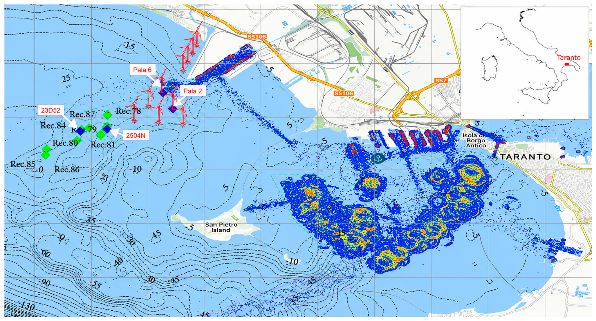
The Port of Taranto is one of the largest, oldest, and most strategic maritime hubs in Southern Italy. It serves as a major commercial and industrial port, as well as a popular cruise destination. Taranto is also the main base for the Italian Navy. A snapshot of average marine traffic, reconstructed from the Automatic Identification System (AIS) used on ships and by vessel traffic services, is shown in Figure 1. To ensure safe harbour operations, vessels strictly follow two fixed traffic lanes to enter and exit the port. The East channel (350 m wide) is used exclusively for entering, while the West channel (300 m wide) is used for exiting. The main freight traffic, therefore, passes approximately 6 Km from the wind farm and the measurement location. It is important to note that not all marine traffic uses the AIS, which is primarily installed on commercial vessels over 300 GT, passenger ships, and large cargo ships. In addition, military vessels often switch off the AIS, as under international maritime law, naval and government ships are generally exempt from tracking requirements.

Another important factor to consider is that while ships at anchor have their generators running, they do not necessarily have their main engines and propellers active. As shown in Figure 1, there is maritime traffic near the Beleolico wind farm, although this generally consists of smaller fishing boats.

From the perspective of underwater noise generated by marine traffic, it is important to note that sources such as large cargo vessels are confined to the Mar Grande area, the large natural bay that includes the city’s harbour and is enclosed by the Cheradi Islands and protected by major port breakwaters. These breakwaters partly shield the study area from the propagation of underwater noise from marine traffic in the Mar Grande. Similarly, between the Beleolico wind farm and the northern part of the port, there is also a breakwater that reduces the propagation of underwater noise from local maritime traffic and onshore port activities.

2.3. Measurement Setup and Strategy

To study the emissions of the Beleolico wind farm in terms of underwater noise, we adopted a strategy comprising three activities: (i) initial reconnaissance surveys along a transect at increasing distances from the wind farm, using high-accuracy measuring instruments, to understand the overall soundscape of the designated area and to identify suitable locations for subsequent recordings; (ii) a long-term monitoring campaign conducted from 13 June 2025 to 31 July 2025 at two locations—one positioned closer to the tip turbine of the wind farm, and one located further away from it—aiming to measure long-term variations in the soundscape of the designated area and to correlate them with several natural and anthropogenic factors contributing to the Sound Pressure Levels (SPLs) in the area; (iii) synchronous recordings taken at 1 m and 5 m from two different turbines (Pala2 and Pala6) from 30 July 2025 to 31 July 2025, for a total of 30 h, to capture turbine noise to be used in future research as source signals in modelling noise propagation in the designated area.

This approach was also determined by the available technologies. High-quality recordings were made with an acquisition system that must be operated in dry conditions from the ship deck and with hydrophone cables of limited length (see next section).

The long-term monitoring campaign and the synchronous recordings were carried out using sea-bottom recorders that operated independently on batteries, were suspended approximately 2 m above the sea floor and were recovered at the end of the recording period.

2.3.1. Initial Reconnaissance Surveys

The exploratory reconnaissance measurements were conducted during two survey campaigns: (i) a preparatory campaign and (ii) a main reconnaissance campaign.

During the first survey, it was necessary to address several logistical and administrative issues, including those arising from proximity to a military base. A test recording chain was also deployed, which enabled the identification and resolution of several problems related to the system’s power supply.

During this period, we were also able to gather information needed to determine the optimal locations for the deployment of the synchronous period survey planned for a later stage. The activity planned consisted of a series of recordings, each lasting 10 min, taken at various locations at increasing distances from the south-west-tip turbine of the wind farm.

The preliminary survey was also needed to test for potential problems that could arise during recordings due to noise generated by the boat. If noise from the vessel is present, the recordings may be unusable for the project’s objectives; therefore, all potential sources of noise on the ship should be shut down, including, of course, the engine.

This results in the boat drifting, meaning the recording location changes during acquisition and is strongly influenced by currents and winds. It is not possible to use any form of anchoring to prevent drifting, as this would also generate noise.

Since the vessel is adrift, safety concerns arise when near the turbines, necessitating the establishment of a minimum safety distance to avoid collisions. This distance is difficult to define, as it depends heavily on the meteorological conditions on the day of recording. During the preparatory phase, we measured drifts of up to approximately 300 m during the 10 min recordings.

As a reasonable compromise between safety and the ability to effectively record noise close to the turbines, a minimum distance of 500 m from the turbine was chosen for the initial reconnaissance survey’s recording activities.

Another effect of the sea current is that the reported hydrophone depths during these recordings must be considered theoretical, as they were measured from the cable length, meaning the actual depths were likely to be less.

This suggested, during subsequent activities, the use of a CTD (SonTek/YSI CastAway, 9940 Summers Ridge Road, San Diego, CA 92121-3091, USA) to determine depths and also to provide information on the thermocline.

Exploratory Reconnaissance Measurement Instrumentation

During the preparatory and main reconnaissance campaigns (

Table 1. Timing, location and depth of reconnaissance campaigns recordings.

Date	Time	Rec N°	Start Position	End Position	Sea-Bottom Depths (m)	Hydrophone Depths (m)
11/6/2025	16:41	78	40.480507 17.121273,	40.481842 17.120865,	11	5
	17:02	79	40.484085 17.121415,	40.484732 17.121518,	19	10
	17:51	80	40.479985 17.115863,	40.48066 17.117027,	20	18
	18:13	81	40.479345 17.113747,	40.47965217.114133,	20	5
12/6/2025	16:52	84	40.478247 17.111605,	40.475928 17.11227,	15	3
	17:07	85	40.475928 17.112358,	40.474048 17.112325,	21	11
	17:35	86	40.473265 17.10342,	40.47178 17.103187,	26	2
	17:48	87	40.471463 17.103123,	40.469747 17.102672,	23	11
	18:19	88	40.479482 17.120963,	40.47812717.119743,	12	2

) a high-end Hottinger Brüel & Kjær acquisition system was used which was composed of:

• Calibrated HBK 8104 hydrophones, with integral AC-0034 cable with JP-0108 BNC, and 50 m long cable.
• HBK acquisition system ranging from 0.1 Hz to over 100 KHz (

  Table 2. Specifications of the reconnaissance campaign’s recording system (HBK data sheet).

  Absolute Amplitude Precision, 1 kHz, 1 V		±0.05 dB, typ ±0.01 dB
  Maximum operating static pressure		270 dB (4 × 106 Pa)
  Frequency range		0.1 Hz to 120 kHz
  Receiving sensitivity		−205 dB re 1 V/μPa
  Absolute Maximum Input		±30Vpeak on measurement input without damage
  High-pass filters		−0.1 dB	−10%	−3 dB	Slope
  	Hz −10% analogue high-pass filter 0.7 Hz −0.1 dB digital high-pass filter	0.5 Hz 0.7 Hz	0.1 Hz 0.15 Hz	0.05 Hz 0.073 Hz	−20 dB/dec.
  	Hz −10% digital high-pass filter 7 Hz −0.1 dB digital high-pass filter	5 Hz 7 Hz	1.0 Hz 1.45 Hz	0.5 Hz 0.707 Hz	−20 dB/dec.
  	Hz −0.1 dB analogue high-pass filter	22.4 Hz	15.8 Hz	11.5 Hz	−60 dB/dec.
  	Hz −10% analogue high-pass filter 0.7 Hz −0.1 dB digital high-pass filter	−0.1 dB	−10%	−3 dB	Slope

  reports the details of the recording system).
• Dedicated HBK amplifier nexus.
• HBK software (BK Connect 2024.1 28.1.0.207) to drive and record measurements.

2.3.2. Long-Term Monitoring Campaign

Following the exploratory reconnaissance survey phase, two sea-bottom recorders were deployed at different distances from the wind farm in order to record long-term variations in the soundscape and identify the natural and anthropogenic factors contributing to the Sound Pressure Levels (SPLs) in the area.

A comprehensive modelling and study of noise propagation is planned for a later phase of the SWIM project. Here, we focus solely on the correlation between the noise and its possible sources. From this perspective, given that the wind farm comprises ten turbines, it is beyond the scope of this work to identify and track signals in the near field, as this region features complex wave interactions and interferences. Our approach considers only the far field, where waves reach a stable regime, which is easier to interpret. According to [20,29], most of the primary acoustic energy of underwater noise generated by offshore wind farms is concentrated below 1000 Hz, with energy reported down to 44 Hz. To capture these frequencies, and following a precautionary rule of thumb that places the transition zone at twice the wavelength of low-frequency signals, we identified two locations for long-term recordings that also presented seabed conditions suitable for deployment. Site 2504N is closer to the tip turbine of the wind farm (SW) with a distance of 741 m from it, while site 23D52 is located further away, with a distance of 1383 m from the tip turbine (see

Table 3. Characteristics of long-term and synchronous recording campaigns.

Sites	23D52	2504N	Pala2	Pala6
Location	40.4788833333 17.1133333333,	40.4796166667 17.1211833333,	40.4859205330 17.1404847617	40.4908869 17.1432982316
Distance from SW-tip turbine	1383 m	741 m	5 m	1 m
Deployment depth	18 m	9 m	8 m	13 m
Sensitivity	−155 dB re 1 V/μPa	−152 dB re 1 V/μPa	−176 dB re 1 V/μPa	−176 dB re 1 V/μPa
Recording duration	15 min	15 min	15 min	15 min
Recording schedule	Every hour	Every hour	Every 15 min	Every 15 min
Recording start	13 June 2025 15:14	13 June 2025 13:04	30 July 2025 09:59	30 July 2025 08:59
Recording end	3 August 2025 04:14	28 June 2025 23:05	31 July 2025 14:59	31 July 2025 13:59
Sampling frequency	192 KHz	192 KHz	96 KHz	96 KHz
File dimension	345 MB	345 MB	172 MB	172 MB
Number of recordings	1187	Not usable	116	116
Dataset dimension	399 GB		19 Gb	19 GB

).

Only after recovering the instruments did we realise that, unfortunately, site 2504N enclosure had severe leakage problems, resulting in corrupted data. This event prevented us from comparing recordings from two different locations in the designated area, but it compelled us to extend our strategy by developing an alternative approach to maximise the information we could extract from what was available.

As mentioned above, the third segment of the pipeline analysis provided data from two additional sea-bottom recorders positioned close to the turbines. Although these were intended to record a reference source for future work on wave propagation modelling, there was an overlap in the timing of these recordings with those from site 23D52, which led us to think they could be used to draw correlations and considerations.

Long-Term and Synchronous Recordings Instrumentation

The locations, timing and system settings of the two sea-bottom recorders are reported in Table 3. The data acquired during these campaigns were subject to careful quality control and underwent extensive file format checks. Site 23D52’s files exhibited a transient noise at the beginning of the recordings (200 msecs) that have been removed. The timing of the recordings was later checked in order to allow comparison and correlation with other information related to the possible sources of noise. The calibration and sensitivity of the recorders were set by the manufacturer.

3. Results

Although preliminary, the study allows us to disentangle, from the array of different sources of underwater noise, the main ones in the area. Using the wind regime as a proxy for turbine activity [30], we attempted to test for any correlation with noise at different local scales.

As a matter of fact, the power production of wind turbines is proportional to the cube of the wind speed [31], and, at the same time, turbine rotation due to the wind induces vibrations in the turbine structure that result in the generation of noise, which propagates in the designated area [30]. In a simplified approach, if there is a correlation between variations in the wind regime and the recordings, this can be interpreted as evidence of the presence of noise propagating from the turbines; if there is no correlation, this would suggest that the noise is related to other sources.

However, the situation is much more complex. Sound is generated by the wind at sea when waves break due to the interaction of air and the sea surface [32], introducing signals in the same frequency range [33] as that expected from the wind turbines. In addition, the operation of a turbine is not linear with wind speed [34]. Turbines can be idle if the wind speed does not exceed a cut-in value that depends on the design of the turbine and the wind farm. According to [35], typical values for cut-in wind speeds are lower than 5 m/s, for rated wind speeds they are between 5 and 17 m/s, and for cut-out wind speeds they are greater than or equal to 16 m/s. This complicates the possibility of correlating recorded noise with wind farm activity, since the turbines can be idle even if the wind is blowing.

During the timeframe of this study, the average recorded wind speed was 4 m/s with a standard deviation of 2.1 m/s, which means that the cut-in threshold might be an issue for our analysis. Furthermore, no data is available on turbine activity that could be used to restrict the focus to relevant data. At the same time, even when the turbine is idle, standstill vibrations or stall-induced vibrations can generate noise [36].

A recent study [37] correlates high levels of underwater noise below 50 Hz with tides, suggesting that the noise levels should peak 1.5 h before high tide or low tide. Other authors [38], on the contrary, refer to this as non-acoustic turbulent pressure fluctuations (pseudosound) around the hydrophone, which can artificially inflate low-frequency Sound Pressure Levels.

A large number of other possible sources of anthropogenic noise can be captured by the hydrophone recordings, such as ship engines (moving or stationary), airplane passages, or noises from the port such as cranes, power stations, or traffic.

Since most of these noises are not related to the wind regime, it is important to identify and exclude these events from the analysis, as they can bias the correlation with the turbine activities.

3.1. Analysis of the Exploratory Reconnaissance Survey Dataset

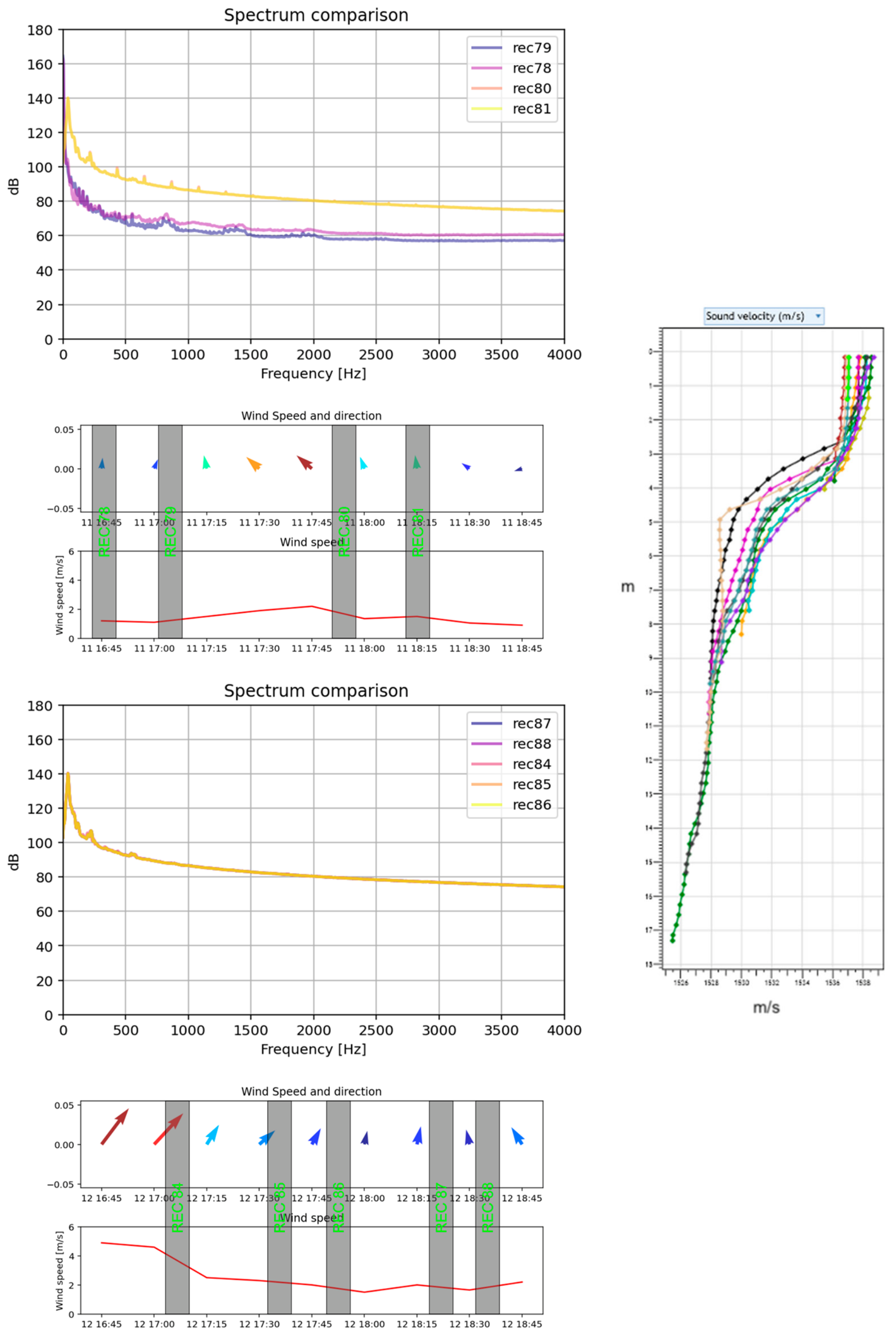
As a first step towards the analysis of the data, we considered the exploratory reconnaissance survey done on 11 and 12 July 2025. Since data were acquired in different meteorologic conditions, in order to keep possible factors separated we decided to analyse the spectra of the recordings, gathering them by date. Recordings done on 12/6 (Figure 2 lower graphs) show overall higher spectrum values with 80 dB at 2000 Hz, while recordings done on 11/6 (Figure 2 upper graphs) show values around 60 dB at 2000 Hz. Interestingly, data recorded on 12/6 show much greater coherence between recordings than those recorded on 11/6; recording 81 shows values comparable with those obtained on 12/6. Referring to the map in Figure 1, it is possible to see that recordings with lower signals (recordings 79 and 78) were made closer to the turbines than, for example, recording 81, which, in the spectra comparison of 11/6, shows the highest values. Referring to Table 2, which reports depths of the sea bottom and depths of the hydrophone deployment for each exploratory reconnaissance survey recording, it is to be noted that those done on 11/6, such as recordings 81 and 78, although both taken 5 m below the surface, express rather different spectrum values; meanwhile, recording 80, which was taken 18 m below the surface, shows spectrum values similar to recording 81, taken 5 m below the surface. Analysing the recordings done on 12/6, it is possible to see that they almost exactly overlap, although also in this case recordings were taken at different depths, ranging from 3 to 11 m.

In Figure 2 (left column) it is possible to see the wind trends recorded by the Italian Institute for Environmental Protection and Research (ISPRA) meteorologic station located at St. Eligio wharf, approximately 7 Km far from the Beleolico wind farm. Data were selected on the timing ranges of the exploratory reconnaissance survey recordings, with the specific time range of each recording highlighted with a grey box to allow easier comparison of spectra and the wind regime. Please note that, for the ease of the reader, the wind direction was plotted with the convention that the tip of the arrow shows where the wind blows towards.

In the right column of Figure 2, the sound profile obtained from CTD casts at each recording location is shown. The mixed layer depth is near the surface (approximately 3 m), and the thermocline is narrow, extending from 4 to 6 m in depth. Additionally, the density profile remains nearly constant throughout the water column. These environmental conditions are likely to promote favourable sound propagation within the water column.

On 11/6 the wind regime showed prevalent winds from S-SE, meaning mostly parallel to the coastline, with rather limited wind speed. On 12/6, higher variability in wind speed was recorded, with a prevalent direction from SW (blowing from the sea toward the land).

Unfortunately, there is no wave monitoring station near the designated site, the closest being in Crotone, which is 150 Km away from the Beleolico wind farm. Therefore, we manually took visual and qualitative notes of the sea conditions, of the depths of the thermocline, and of the movements of the turbines.

This information can be seen in

Table 4. Sea, turbine status and thermocline depth during reconnaissance survey recordings.

Date	Rec N°	Douglas Sea Scale	Turbine Status	Thermocline Depth	Notes
11/6/2025	78	2—Smooth	All moving (0.1 Hz)	4–6 m
	79	2—Smooth	Slowing down (0.05 Hz)	4–6 m
	80	2—Smooth	All stopped	4–6 m	Airplane passage
	81	2—Smooth	All stopped	4–6 m	Airplane passage
12/6/2025	84	3—Slight	All moving (0.16 Hz)	3 m
	85	2—Smooth	All moving (0.16 Hz)	3 m
	86	2—Smooth	All moving (0.16 Hz)	3 m	Large ship (far)
	87	2—Smooth	All moving (0.16 Hz)	3 m	Fishing boat (close)
	88	2—Smooth	All moving (0.09 Hz)	3 m	Fishing boat (close)

and highlights that, during all the exploratory reconnaissance surveys, the sea state, using the Douglas sea scale classification, was of class 2 (smooth) relating to wave heights between 0.1 and 0.5 m, except for recording 84 when the wave height was slightly higher.

It is very interesting to compare the spectra with the actual turbine status as reported in the field notes. On 11/6, the status of the turbines shows a decrease in rotation speed, while during recordings 80 and 81 the turbines were completely idle. Conversely, recording 81 shows the highest spectrum values, which are also very similar to those of the recordings on 12/6. The notes taken during the recordings highlight the presence of an airplane at both stations 80 and 81. On 12/6, the field notes report that all turbines were active, and that a large, distant military vessel was passing by during recording 86, while a fishing boat was passing by during recordings 87 and 88.

3.2. Analysis of the Long-Term Monitoring Campaign Dataset

The original plan for the long-term monitoring campaign was to compare recordings at two sites during a large overlapping timeframe. As mentioned above, this was unfortunately not possible, as site 2504N was flooded. Nevertheless, several observations and considerations can be made by analysing the available data. Also, since the synchronous recordings made near the turbines (Pala2 and 6), originally intended for the future project’s activity of noise propagation modelling, were conducted within the timeframe of the 23D52 recordings, we planned to compare them to the long-term recordings with caution.

In the case of the long-term and synchronous survey, it is not possible to directly correlate spectra with the possible causes of the underwater noise, as there were too many recordings. We will, instead, use the variation in the average SPL [39] among recordings. The SPL is defined in Equation 1 where the reference pressure p_r is 1 µPa.

$$L_P=10{log}_{10}{\displaystyle \frac{\overline{p^2}}{p_r^2}}dB$$

(1)

The sea-bottom recorders used for long-term monitoring stored recordings as 16-bit .wav files directly onto their disc drives. SPL analysis was performed after system recovery by processing all files, reading the values, and normalising them to obtain the actual signal voltage, using the peak-to-peak voltage and gain values provided by the acquisition system manufacturer. Conversion to pressure was carried out using the hydrophone sensitivity specified by the manufacturer during calibration. Each .wav file recorded at each site underwent this processing phase and was associated with a mean SPL value. All SPL values were then time-referenced using the internal clock of the acquisition system and saved in a text file. In subsequent phases of our work, statistics and correlation analyses were performed directly on these files.

4. Discussion

4.1. Visual Inspection of SPL Datasets and Correlation with Wind Regime

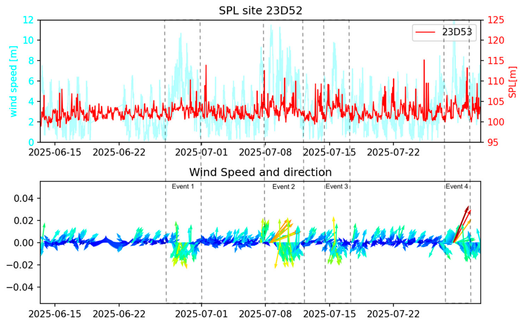
As an initial analysis of the recordings from site 23D52, we correlated the average SPL calculated from each recording with the wind speed and direction recorded by ISPRA during the same period (Figure 3). The time range of the plots cover the period from 13 June 2025 15:14 to 31 July 2025 12:14. Please note that, in the bottom graph of Figure 4, wind direction is plotted using the convention that the tip of the arrow indicates the direction towards which the wind is blowing. By analysing the wind graph, several events can be identified, each corresponding to an increase in wind speed, which on average rises from 3 m/s to 7 m/s, with peaks exceeding 10 m/s. For the reader’s convenience, these four events are highlighted with dashed boxes. Correlations between wind speed and increases in the SPL can be observed for Events 1, 2, and 3, while there is less evident correlation in Event 4.

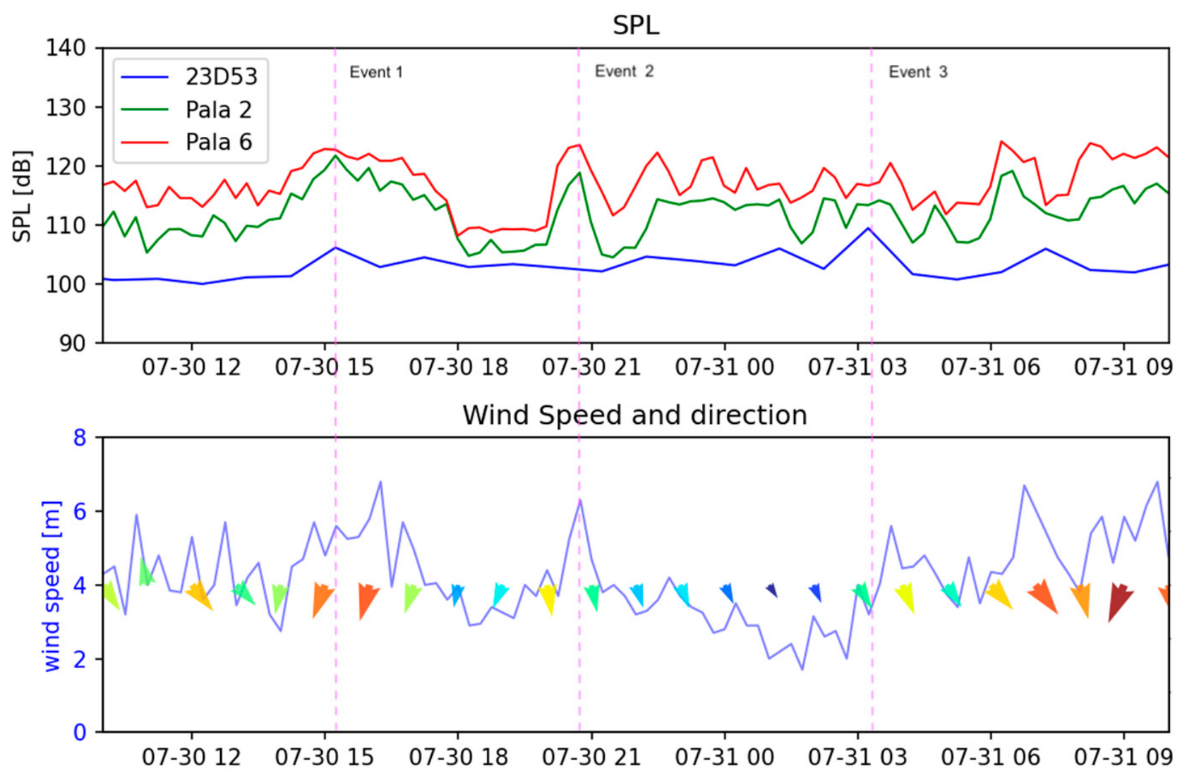
Within the timeframe when the Pala2 and Pala6 recordings were made, there was also a time overlap with data from site 23D52. It is therefore possible to gather all three recordings and compare them with the wind regime. Examining the SPL graphs of the three sites in Figure 4, several observations can be made. Pala6, located 1 metre from the turbine, shows the highest SPL values; Pala2, at a distance of 5 m from the turbine, shows a lower SPL than Pala6 but higher than site 23D52. It is interesting to also note that, in this case, there is a certain correlation between the wind regime and the SPL time series; while the SPL values at the Pala2 and Pala6 sites correspond well with variations in wind speed, site 23D52 shows a less clear pattern. In fact, although the wind speed variations during Events 1 and 3 appear to be reflected in peaks in all three SPL time series, Event 2 shows no evident change in site 23D52’s SPL time series.

4.2. Limitations in the Joint Use of SPL Time Series from Sites 23D52, Pala2 and Pala6

The visual comparison of SPL time series from sites 23D52, Pala2 and Pala6 with the wind regime highlighted inconsistent behaviours. In

Table 5. SPL statistics and expected transmission loss and recorded SPL differences within the time range where sites 23D52, Pala2 and Pala6 overlap.

Site	Min SPL	Max SPL	Average SPL	SPL Standard Deviation	Distance	Transmission Loss (Theoretical)	Δ SPL
Pala6	108.10	124.10	117.13	4.13	1 m	0	0
Pala2	94.44	121.10	111.20	5.40	5 m	6.9	5.93
23D52	99.94	109.40	102.97	1.78	2430 m	33.89	14.16

we gathered the descriptive statistics of those SPL time series. There, Pala6, located 1 m from the turbine, shows the highest values (on average 117 dB); Pala2, at a distance of 5 m from the turbine, shows an average of 111 dB; and site 23D52, within the considered time range, shows an average SPL of 102 dB.

The SPL difference between Pala2 and Pala6 is approximately 6 dB, which, considering the approximate sensor positioning, the effects of nearby turbines, and the variability in the activity of individual turbines, appears reasonable. This aligns with the expected 6.9 dB reduction due to the distance from the source in a simple cylindrical transmission loss model, appropriate for the shallow waters in the area. In contrast, given the distance of 2430 m between site 23D52 and Pala2, the actual SPL difference of only 14.16 dB indicates that a direct comparison of the SPL between recordings from Pala2 and Pala6 with those from site 23D52 is not feasible. The latter is in the far field, and too many other factors contribute to its SPL.

4.3. Spectrograms as a Tool to Identify the Origin of Signals

To understand in detail the causes of the inconsistencies in the SPL time series behaviours, we analysed each specific recording corresponding to each event at each site through their spectrograms.

Following [29,30], a very useful tool for determining whether a noise can be related to wind farm activity is the tonal component shift in the spectrogram. This is a periodic shift in the frequency peaks within the time-frequency representation of the sound signal, which depends on the speed of the turbine rotor and follows wind velocity variations.

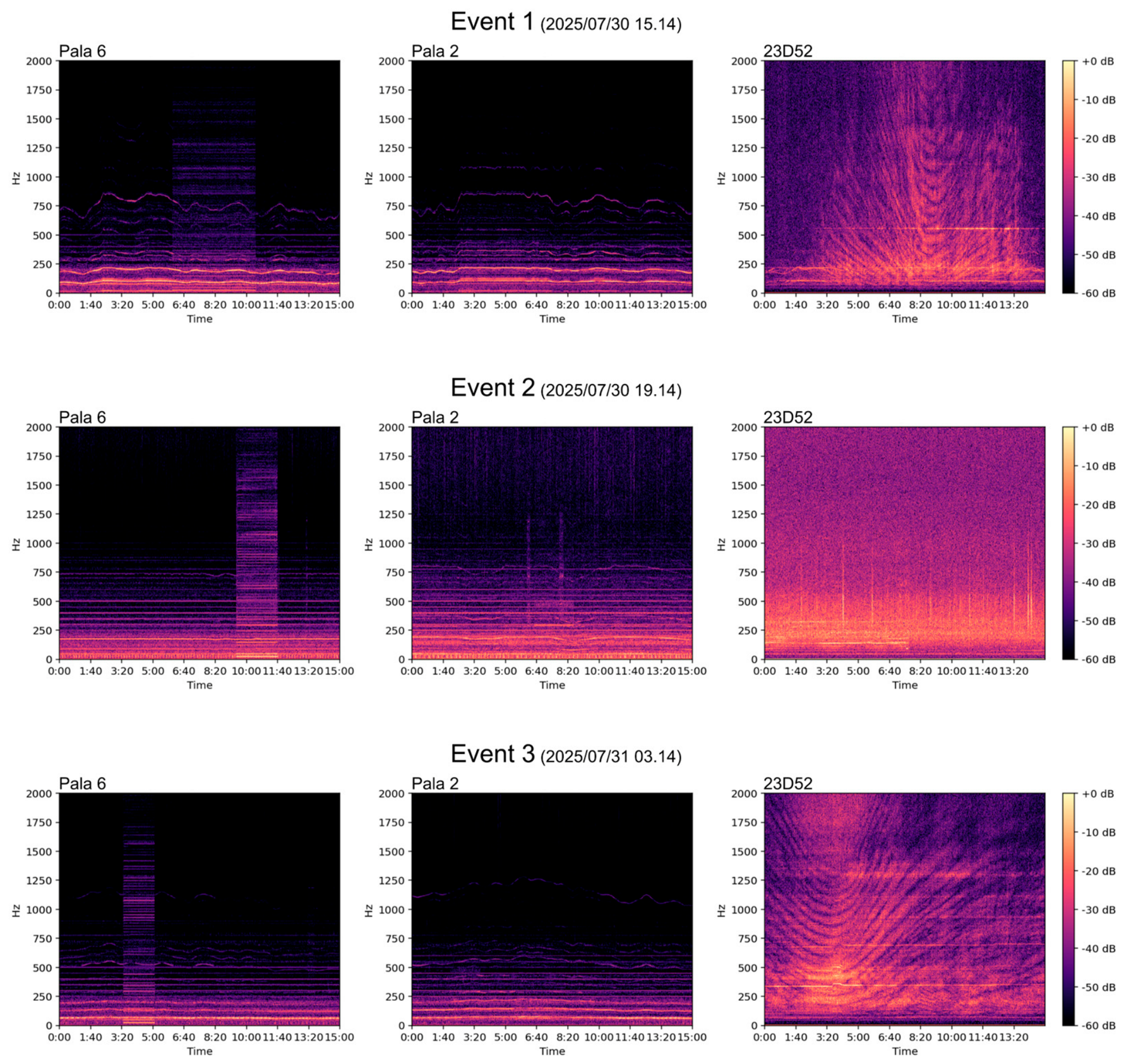
In the case of Event 1, the Pala6 and Pala2 spectrograms (Figure 5) show prominent low-frequency continuous tonal component shifts caused by the turbine activity, with harmonics extending from a few dozen Hertz up to 1000 Hz, unequivocally linking them to the turbine activities. For Event 1, the spectrogram of recordings at site 23D52 shows a prominent Lloyd’s Mirror Effect (LME) event, with the closest point of approach at the ninth minute of the recording. This event considerably increases the overall SPL energy of this recording, while lower energy tonal components can also be visually detected with caution below the stronger LME event.

In the case of Event 2, which corresponds to a short-lasting increase in wind speed, while the Pala2 and Pala6 spectrograms show relatively stable tonal components, the 23D52 site shows almost no coherent signal.

Event 3 presents a situation very similar to Event 1, with a large LME at site 23D52, while rather stable tonal components are recorded at Pala2 and Pala6.

Spectrograms of the specific events considered highlight that peaks in the SPL time series at site 23D52 were strongly influenced by other sources of noise, probably boats or airplanes passing by. In contrast, sites Pala2 and Pala6 are mostly influenced by the high-energy noise due to vibration from the nearby turbines. Although there appears to be a correlation between the SPL peaks of Events 1 and 3 at site 23D52, this analysis shows that these cannot be directly attributed to the activity of the wind farm.

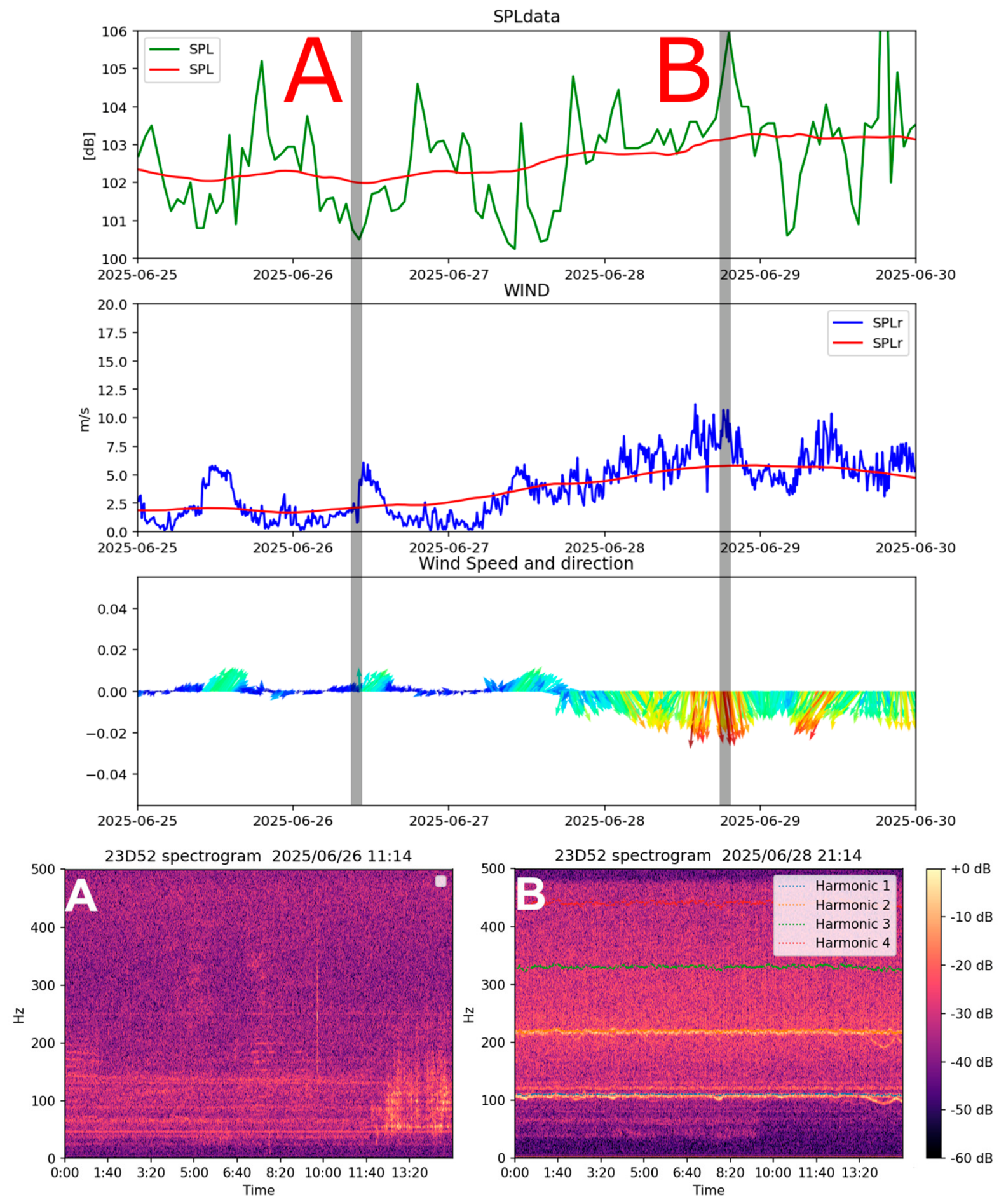
As we have seen in Section 4.1 and Figure 3, considering the full range of recordings done at site 23D52, there are four events where there is a correlation between the increase in the speed of the wind and the increase in the SPL. Figure 6 (upper) shows a zoomed-in version of Figure 3 for Event 1, highlighting the onset of the increase in the SPL corresponding to an increase in wind speed. In order to understand whether this increase in the SPL is linked to an increase in the turbine activity, we selected two recordings—namely recording A, corresponding to low SPL and wind speed values; and recording B, corresponding to a high SPL value. The spectrograms of these events (Figure 6) show that no tonal component is evident during recording A, while tonal components can be clearly identified during recording B. To quantitatively estimate the harmonics visible in the spectrogram, we used the Probabilistic YIN (PYIN) algorithm [40,41]. This algorithm is a highly robust estimator of the fundamental frequency, especially in cases of frequency variations such as the tonal tuning associated with turbine activity. The PYIN computes multiple pitch candidates and provides the probability of detection. In our case, while the algorithm was unable to provide solutions for recording A, it produced reliable results for recording B. The fundamental frequency ranged from a minimum of 106.78 Hz to a maximum of 112.48 Hz, with a mean value of 110.07 Hz and a standard deviation of 0.85. The variation in frequency of the fundamental harmonic supports the hypothesis that this noise is generated by the wind farm.

Similar observations have also been reported by [29] where strong tonal components were observed at frequencies of approximately 99 Hz along with harmonics at 198, 297 and so on, when the wind speed was higher. They also noted that the 198 harmonics had the strongest energy. Similarly, in our case, the second harmonic, at approximately 220 Hz, shows higher energy that the fundamental one.

The overall difference in the average SPL between recording A and B is approximately 5 to 6 dB.

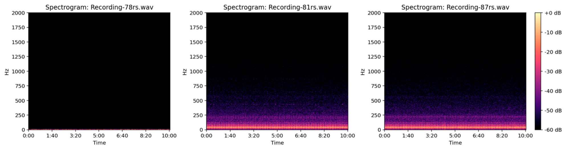
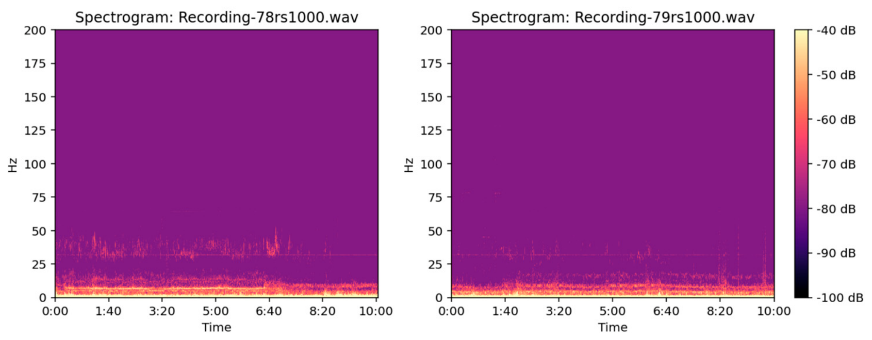
As mentioned in Section 3.1, the trends in the exploratory reconnaissance survey recording showed rather erratic behaviour. The large differences in the spectra shown in Figure 2 are not easily correlated with any possible factor affecting the energy of the signal. However, listening to the .wav files, it is evident that from recording 80 onwards a high-amplitude periodic signal is present that cannot be heard in recordings 78 and 79. This signal cannot be correlated with the turbine activity, as the wind did not change significantly, and the field notes report the turbine slowing down to idle. On 12/6, the field notes report active turbines, which at first sight could explain the higher spectra. However, referring to Figure 7 and Figure 8, which compares the spectrograms of three recordings (78, 81, and 87), the similarity between recordings 81 and 87 suggests a different source of noise. The field notes report the passage of an airplane during recording 81, but that would leave an LME, which cannot be seen in the spectrogram. A more reasonable explanation would be the presence of a large vessel that switched on its engines between recordings 78 and 80 and kept them running throughout 12/6. This would also explain why all these recordings have almost the same spectrum: it is probably the signature spectrum of the vessel’s engine.

4.4. Analysis of the SPL Time Series at Site 23D52

As mentioned above, unfortunately, we can rely only on one of the planned far-field SPL time series to understand the sources of underwater noise in the designated area, as data from site 2504N are not usable. In addition, in Section 4.2 we explained that it is not advisable to correlate the SPL time series from site 23D52 with those in the near field (Pala2 and Pala6). We therefore focused on the analysis of the 23D52 recording with the aim of identifying periodicities in the SPL time series and, where possible, linking them to potential sources of underwater noise.

4.4.1. Statistics of Available Data

As a first step towards correlating the noise dataset with its possible sources, we gathered data on wind speed and direction, as well as on tides. Regarding wave monitoring, as mentioned previously, there is no useful information available, as there is only one station monitoring the sea wave state in that region of Italy, but it is too far away to provide useful information.

Table 6. Descriptive statistics of the available datasets.

Dataset	n. Points	Mean	Std. Dev.	Min	25%	50%	75%	Max
23D52	1218	102.5 dB	1.84 dB	98.6 dB	101.2 dB	102.3 dB	103.4 dB	115.2 dB
Wind vel. 1	5042	3.35 m/s	2.13 m/s	0.1 m/s	1.7 m/s	3.0 m/s	4.7 m/s	12.3 m/s
Tide 1	5042	−0.12 m	0.07 m	−0.30 m	−0.17 m	−0.12 m	−0.07 m	0.12 m

¹ The wind and tide datasets have two gaps in the recordings, probably due to a malfunction of the station.

presents descriptive statistics of the datasets we will use. It should be noted that the different datasets have different sampling rates. The SPL for site 23D52 contains values taken every hour, while the datasets at sites Pala2 and Pala6 report the average SPL every 15 min. The wind and tide datasets sample data every 10 min and, probably due to a malfunction of the acquisition system, show two gaps in the recordings: from 18 June 2025 22:10 to 22 June 2025 10:40, and from 27 July 2025 11:50 to 28 July 2025 08:10.

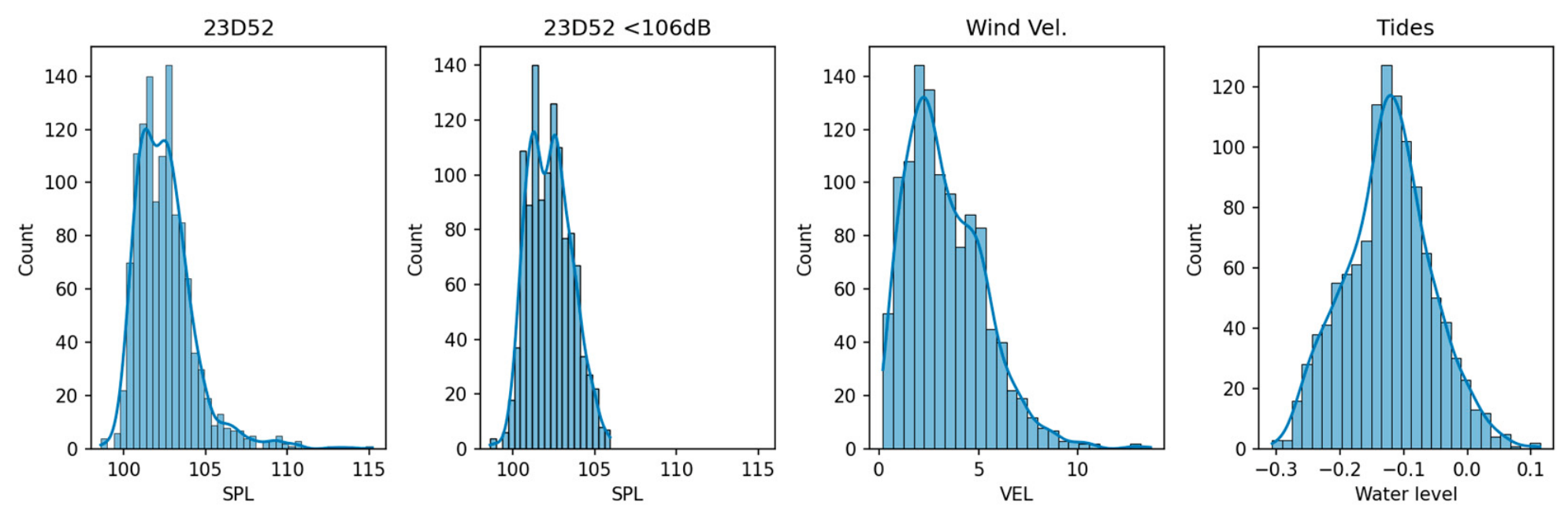
To assess whether the datasets are normally distributed, Figure 9 and

Table 7. Skewness and kurtosis of the available datasets.

Dataset	Skewness	Excess Kurtosis	Z-Score
23D52	1.83	6.39	12.98
23D52  1	0.30	−0.41	−3.67
Wind Vel.	0.86	0.53	6.18
Tides	0.086	−0.05	−0.29

¹ SPL dataset excluding events above 106 dB.

present the skewness and kurtosis of the available datasets. The site 23D52 SPL time series and the wind velocity time series display considerable asymmetry, suggesting the presence of outliers in the datasets. Both the site 23D52 SPL dataset and the wind velocity exhibit positive skewness, while the z-score using the Anscombe–Glynn transformation indicates that the kurtosis is significantly different from that of a normal distribution. As our aim is to correlate the SPL and wind velocity, excessive skewness and kurtosis in these datasets can cause disproportionality due to outliers or spurious correlation due to time series skewed in the same direction. In contrast, the tide dataset can be interpreted as normal.

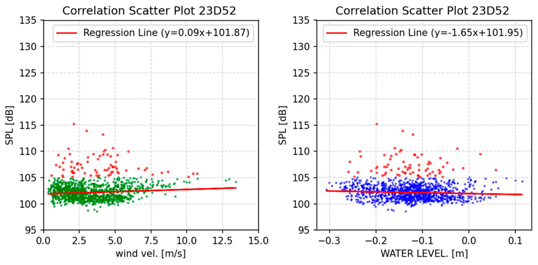
To understand how the acquired SPL datasets correlate with the wind speed and tide time series, we cross-plotted them (Figure 10). Linear regressions were derived, and the Residual Standard Error (RSE) was calculated to evaluate the goodness of fit of the linear regression model. The RSE represents the standard deviation of the residuals, measuring the average distance of the observed data points from the predicted regression line. The linear regression parameters and the RSE for all correlations are reported in

Table 8. Linear regression parameters and Residual Standard Error (RSE).

	Slope	Intercept	RSE
23D52/wind speed	0.12	102.10 dB	1.80 dB
23D52 1/wind speed	0.09	101.87 dB	1.22 dB
23D52/tide	−2.09	102.23 dB	1.81 dB
23D52 1/tide	−1.65	101.95 dB	1.23 dB

¹ SPL dataset excluding events above 106 dB.

. The regression of the raw SPL with wind speed and water level yields an RSE of 1.80 dB and 1.81 dB, respectively.

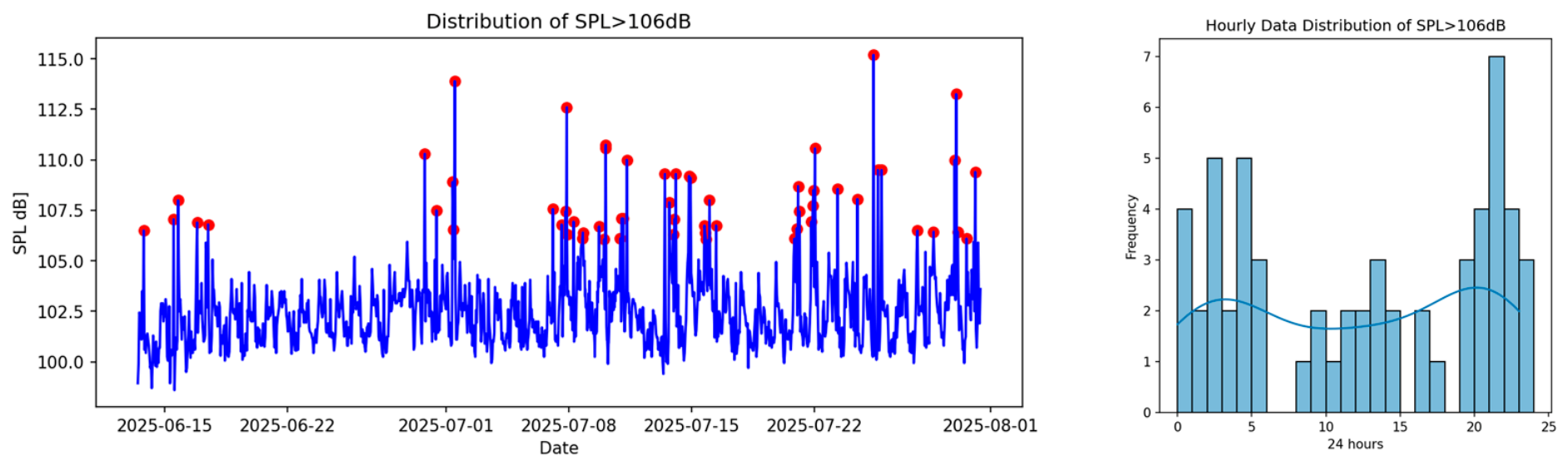
A visual examination of the graphs in Figure 10 shows strong coherence among most points, except for several outliers above approximately 106 dB. Excluding these data from the regressions reduces the RSE to 1.22 dB and 1.23 dB, which is an even better error of approximately 1%. The question of what these points correspond to is interesting.

It should be noted that these high SPL values often correspond to low wind speeds and therefore cannot be related to turbine activity. As a first step, we can plot them together with the full site 23D52 SPL dataset (Figure 11, left). At first glance, they appear to be randomly distributed. However, plotting a histogram of their distribution by hour of day reveals two peaks, one around 9 p.m. 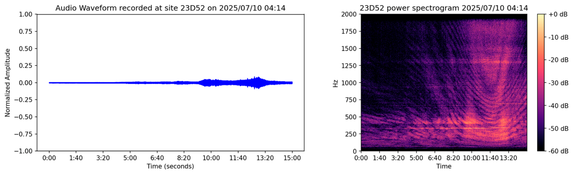and the other at the very beginning of the day (Figure 11, right). Once these points were identified, we conducted a direct examination of all 58 highlighted recordings. As an example, we present the file acquired at site 23D52 on 10 July 2025 at 04:14 a.m. This file shows a prominent increase in amplitude after five seconds, corresponding to the onset of a Lloyd’s effect visible in the spectrogram (Figure 12), which can be unequivocally identified as the passage of a boat—a conclusion also confirmed by hearing the distinct signature of the boat engine in the file. All recordings containing high SPL events are characterised by the same situation. Considering the two peaks in the distribution of these events throughout the day, it is probable that these events can be associated with fishing boats departing and returning to the port. If this interpretation is correct, and we aim to highlight the correlation between the SPL and wind as a proxy for turbine activity, we can remove these data from the SPL time series. After removal, the skewness and kurtosis of the SPL time series are significantly reduced. In fact, the skewness decreases from 1.83 to 0.30, and the excess kurtosis drops from 6.39 (z-score 12.98) to −0.41 (z-score −3.67).

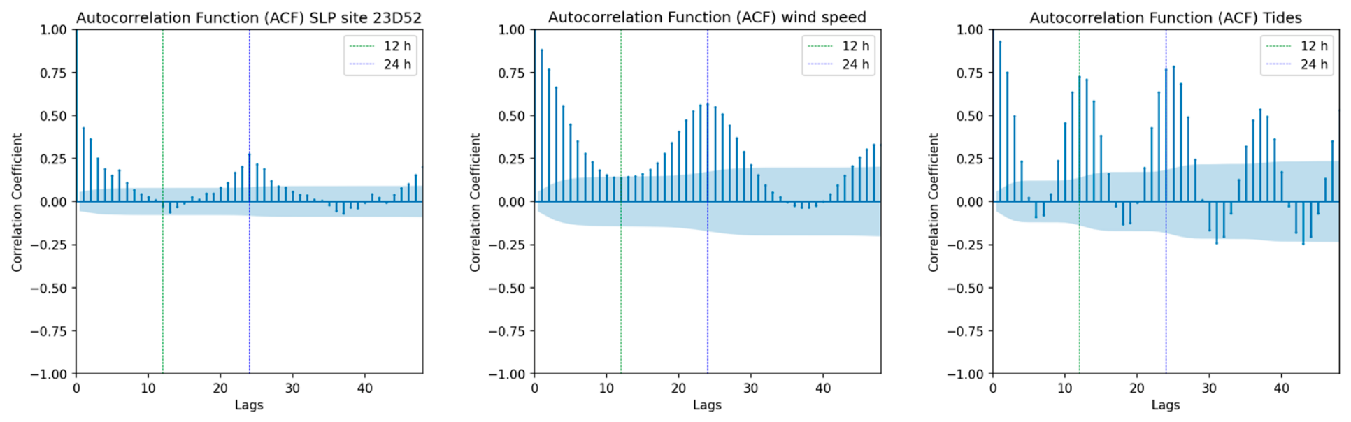
Once recordings that can be associated with fishing boat passages have been removed from the SPL dataset, we can highlight periodicities in the dataset and check whether these periodicities can also be found in the other datasets. Figure 13 shows the autocorrelation function (ACF) of the SPL dataset at site 23D52 of the wind speed and tides datasets. Tide periodicity as expected is 12 h and 25 min, while both wind speed and SPL ACFs demonstrate periodicities of 24 h.

Recent studies [37] correlate high levels of underwater noise below 50 Hz with tides, suggesting that the noise levels should peak 1.5 h before the high tide or low tide. Other authors [38], on the contrary, refer to this as non-acoustic turbulent pressure fluctuations (pseudosound) around the hydrophone, which can artificially inflate low-frequency Sound Pressure Levels. In the case of our study, the SPL autocorrelation of site 23D52 (Figure 13, left) does show a semi-diurnal periodicity as a negative peak which is nonetheless located within the 95% confidence interval (light blue area), suggesting the influence of tide flows on the SPL dataset should not be strong.

Following the studies of Isaak Van der Hoven [42], the power spectrum of horizontal wind speed is made over a wide range of frequencies with two major energy peaks, namely (i) one with a period of 4 days that represents large-scale weather systems such as the passage of high- and low-pressure fronts and (ii) another peak corresponding to the solar heating and cooling that has a 24 h periodicity. Van der Hoven also introduced the concept of a mesoscale spectral gap, with a period between 6 min and one hour, which is a region in the spectrum where wind energy is at its minimum, indicating an absence of significant atmospheric processes. The wind speed spectrum also shows a turbulent peak with a period of a few minutes. This is a range of periodicities that can be problematic for wind turbines because it can generate structural loads that can affect their lifespan. Since the sampling rate of the considered SPL is one hour, we doubt that these periodicities can be identified in the data.

4.4.2. Seasonal–Trend Decomposition

Since the SPL show a diurnal and semi-diurnal peak in the autocorrelation that can be associated with the wind and the tide, we aimed at isolating these trends in the SPL time series. To understand whether the time series are stationary we used the Augmented Dickey–Fuller algorithm which tests whether the time series has a constant mean, variation and autocorrelation. The ADF test has been performed using Schwert’s criteria for the maximum lag. Results of the test show that the SPL dataset can be considered stationary (p-value less than 0.05, ADF more negative than 5% critical value) while the wind speed dataset cannot (p-value above 0.05, ADF higher than all critical values).

To isolate the periodicities in the SPL dataset we used a seasonal and trend decomposition employing Locally Estimated Scatterplot Smoothing (LOESS) [43,44].

This is a filtering procedure for decomposing a time series into trend, seasonal and remainder components which essentially consists of a sequence of applications of the LOESS smoother, which is a non-parametric method that can fit a smooth curve through a noisy scatter plot making no assumptions about the overall shape of the data but relying on localised, weighted regression to capture non-linear trends. An important feature of the method is that it can deal with missing values such as those in the wind speed and tide datasets, and it can also deal with anomalous points (robustness).

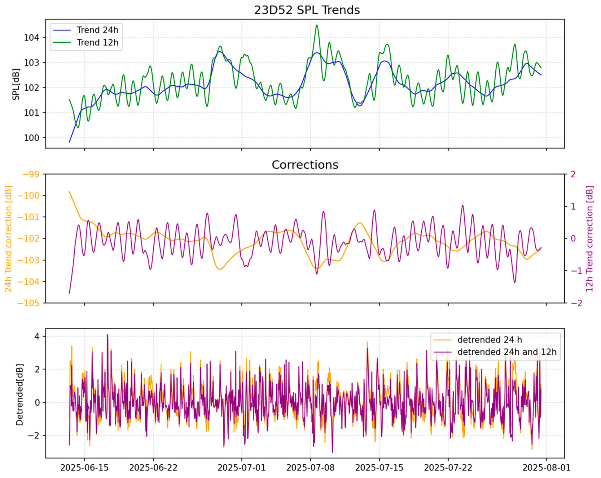
We applied the LOESS algorithm to the 23D52 SPL time series two times. The first run aimed to derive the diurnal periodicity, while a second run aimed to reconstruct the semi-diurnal periodicity. The extracted periodicities can be used both as trends to correlate with the wind and tide, and also as a correction to detrend the SPL time series. Figure 14 shows the results of the application of the LOESS algorithm, where in the upper graph the diurnal and semi-diurnal trends are plotted. The graph in the middle shows how they can be used as a correction to detrend the original SPL time series to obtain (lower graph) the progressively detrended residuals.

4.4.3. Correlation of SPL, Wind Regime and Tides

Since, in Section 4.1 and Figure 10, the correlation of the SPL at site 23D52 with wind speed and water level showed a rather high goodness of fit in the linear regression model, it is possible to use the Pearson correlation coefficient r to evaluate the strength and direction of the linear relationship between these parameters and their decomposed versions. A summary of these results is presented in

Table 9. Correlation between original and decomposed datasets.

Dataset	Dataset	r	p-Value
SPL trend 24 h	Wind vel. trend 24 h	0.6991	0.0000
SPL trend 12 h	Water level trend 12	0.6289	0.0000
Raw SPL	Raw wind vel.	0.1522	0.0000
Raw SPL	Water level	−0.0876	0.0030

. Although it is not easy to observe a direct correlation between the raw time series of the SPL and wind velocity and water level, considering the decomposed time series, the correlations increase significantly. In the case of the 24 h trend of the SPL and wind speed, the correlation coefficient rises to almost 0.7.

Table 10. Tests for stationarity of the available datasets.

Dataset	ADF	p-Value
23D52	−3.34	0.012	Stationary
Wind	−2.22	0.1967	Non-stationary
Tide	−4.29	0.0005	Stationary

also shows the p-value of the correlation, which indicates the statistical significance of the correlation. When the p-value is less than 0.05, there is strong evidence that a relationship likely exists overall. In the case of the correlation between the 24 h trend of the SPL and wind speed, the p-value is negligible, indicating that the statistic is significant. In Figure 14, the diurnal trend of the SPL can be observed, which ranges from approximately 4 to 5 dB (see

Table 11. Descriptive statistics of the raw 24 h detrended SPL time series and a possible estimate of the 12 h trend.

Dataset	Mean	Std. Dev.	Min	25%	50%	75%	Max
SPL trend 24 h	102.1 dB	0.57 dB	99.8 dB	101.7 dB	102.0 dB	102.5 dB	103.4 dB
SPL resid. 24 h	0.11 dB	1.84 dB	−2.84 dB	−0.8 dB	0.06 dB	0.8 dB	3.9 dB
SPL trend 12 h	0.11 dB	0.43 dB	−1.03 dB	−0.18 dB	0.1 dB	0.4 dB	2.51 dB

). Detrending the raw SPL time series with this 24 h component, the residuals are expected to incorporate the semi-diurnal tide components, turbulent wind peaks, and other components which are more difficult to identify. Overall, these residuals have approximately the same spread as the diurnal trend. A semi-diurnal component can be identified in these residuals, which can be linked to the tides that range approximately 3 dB.

Similarly to the case of the 24 h trend, the 12 h trend of the SPL derived from the residuals correlates significantly with the 12 h water level trend. Here, we highlight a problem arising from the fact that at site 23D52 data was acquired every hour. Since the tidal periodicity is 12 h and 25 min, this creates a progressive shift relative to the SPL sampling time that, despite the high r value, does not allow for a good match between the SPL and tide trends. In fact, while the 24 h periodicity linked to wind speed can be well isolated and its impact on the overall SPL time series evaluated, the 12 h periodicity related to tides can be problematic with the currently available SPL sampling rate. Under these conditions, it could be risky to provide definitive values for the wind component in the SPL; rather, it is safer to estimate approximately what that component can induce. From Table 10, we can say that, in the timeframe of the survey, at site 23D52, the wind speed trend can induce up to a 5 dB increase in the SPL. The detrended residuals, which have approximately the same range as the wind-linked trend with the limitation of the 1 h SPL sampling, tentatively provide a diurnal trend ranging from 2 to 3 dB, while the final residual can be associated with turbulent wind effects as well as other noise sources.

5. Conclusions

Supported by preliminary evidence, analysis of the data recorded within the SWIM project highlighted that the Beleolico wind farm may generate underwater noise that propagates from the turbines to the open sea and can be detected at least up to 1383 m from the south-west tip of the wind farm. At that location, a hydrophone was deployed which recorded the soundscape of the designated area for almost 50 days, allowing the definition of a long-term SPL time series. Anomalous events linked to the passage of boats have been identified and filtered from the dataset. Similarly, tidal effects have been removed from the time series using semi-diurnal seasonal decomposition, resulting in a residual time series that can be correlated with the wind regime. In the absence of wind and with stationary turbines, the average recorded SPL reaches approximately 100 dB. Increases in wind speed correlate well with increases in the SPL, and the direct link between SPL increases and wind farm activity has been demonstrated by the presence of tonal component shifts in the spectrograms. The presence of such features allows us to separate events linked to the turbine activity from other contributors to the SPL such as marine traffic or, for example, from breaking waves and bubbles. Following [33], the spectrum of these latter sources ranges from a few hundred Hz up to 100 kHz and, being a random process, it does not show tones in the spectrum.

Our analysis showed that, during the recording period, increases in wind speed exceeded 10 m/s. We estimated that in such cases the increase in the SPL can reach approximately 6 dB. The analysis confirms that all underwater noise produced by the turbines is confined below 1000 Hz and that, as the distance between the receiver and the turbines increases, together with a reduction in sound intensity, absorption narrows the spectra so that at the 23D52 deployment location most of the energy is confined below 300 Hz.

Limitations and Future Work

Our work was significantly affected by the malfunction of one of the two planned recording sites. As a result, we were unable to characterise underwater noise by comparing SPLs at different locations, as originally intended. Additionally, other recordings made near the turbine to capture its source signature for future research, although within the timeframe of the main recordings, proved not to be suitable for direct comparison with the long-term recordings. Nevertheless, preliminary evidence seems to support the strategy behind the SWIM survey and corroborates the thesis on the presence of underwater noise originating from the Beleolico wind farm at the 23D52 recording site. From this perspective, we are confident that a future round of recordings based on the same strategy and employing the methods developed in this work could address the difficulties we encountered so far. Future surveys will also be supported by the wave propagation modelling activity planned during the next phase of the project. In that phase, the recorded turbine signature, together with all the information on turbine hardware and geophysical information acquired during this stage, will be used to build an acoustic model of the designated area, which will be validated by the future recordings.