Research of Sound Speed Field Spatiotemporal Variations in the Central Philippine Basin

Abstract

The Philippine Sea Basin is one of the world’s largest marginal sea basins, and the spatiotemporal variation characteristics of its sound speed field hold significant importance for deep-sea navigation and positioning as well as underwater acoustic detection. This study investigates the sound speed field in the central Philippine Basin (130.0–134.0° E, 17.5–20.5° N) using the Global Ocean Physics Analysis and Forecast product from the European Union’s Copernicus Marine Environment Monitoring Service (CMEMS), cross-validated with the U.S. HYCOM (Hybrid Coordinate Ocean Model), and independent verified against 69 Argo profiles. We systematically investigate the spatiotemporal variation characteristics of the sound speed field in this region. Temperature and salinity consistency between the two products is established (deviations of <0.5 °C and <0.05 ppt below 400 m), with CMEMS selected as the primary data source for its higher accuracy and greater temporal stability. Three sound speed formulae—Del Grosso, Chen–Millero, and TEOS-10—are intercompared, with TEOS-10 yielding the highest accuracy in cross-validation; it is therefore recommended for its rigorous thermodynamic consistency. Vertical sound speed profiles are evaluated using bi-exponential, Munk canonical, and fourth-order polynomial models. Among them, the bi-exponential model achieves the optimal balance between physical interpretability and fitting accuracy (RMSE = 2.77 m/s, inter-monthly correlation coefficient = 0.857). Its two exponential decay scales characterize the upper-ocean thermocline and the deep stratification, respectively, avoiding the physically unrealistic deep-water fluctuations exhibited by the polynomial model (RMSE = 2.68 m/s) and the poorer generalization of the Munk model (RMSE = 2.97 m/s). Horizontal gradient analysis reveals a cross-directional correlation of approximately 0.5 between sound speed gradients and ocean currents, reflecting the combined modulation of sound speed gradients by Kuroshio advection and thermodynamic stratification. The general gradient control scale is estimated at approximately 100 km × 100 km, confirmed by cross-method consistency between K-means and Gaussian mixture model clustering. Temporal analysis demonstrates that sound speed peak-to-peak variation attenuates rapidly with depth (from ~8.9 m/s at 50 m to <0.1 m/s at 4000 m), and EOF (empirical orthogonal function) analysis reveals that the first four modes explain over 99% of the total variance, with harmonic fitting identifying annual and semi-annual cycles as the dominant periodic components. Sound channel axis depth varies seasonally between 900 and 1125 m (deeper in winter, shallower in spring), with axis sound speed stable at 1480–1484 m/s (slightly higher in winter, slightly lower in spring) and axis thickness ranging from 225 to 450 m (wider in winter, narrower in spring). These results provide prior critical constraints for underwater acoustic positioning, AUV navigation, and long-range sound channel communication and navigation in the central Philippine Sea region.

1. Introduction

The ocean sound speed field describes the spatial and temporal distribution of the speed of sound in seawater and constitutes a fundamental physical property governing underwater acoustic propagation. Sound speed in the ocean is primarily determined by temperature, salinity, and hydrostatic pressure (depth); its spatial and temporal variations directly control the refraction, reflection, and transmission loss of acoustic waves, thereby influencing sonar detection performance, underwater acoustic communication link budgets, and the accuracy of marine acoustic positioning and navigation [1,2,3]. In marine science and engineering applications, a quantitative understanding of the spatiotemporal characteristics of the sound speed field is essential for deep-sea navigation and positioning, ocean acoustic forecasting, underwater communication system design, and autonomous underwater vehicle (AUV) operations [4].

The Philippine Sea, located at the western margin of the Pacific Ocean, is the largest marginal sea basin in the western Pacific, surrounded by island arcs and trenches. Its oceanographic environment is highly dynamic, influenced by the Kuroshio Current, the North Equatorial Current, and mesoscale eddy activity, which together produce complex and strongly varying sound speed fields [5]. Systematic investigation of the sound speed field in this region carries both scientific significance—advancing the understanding of western Pacific marginal sea acoustics—and practical importance for improving underwater navigation and positioning capabilities in a strategically important maritime area.

The Philippine Basin, as part of the western Pacific warm pool (WPWP), is characterized by the highest sea surface temperatures in the global ocean (>28 °C), which drive intense air–sea heat flux and deep atmospheric convection [6]. The upper-ocean circulation in this region is dominated by the westward-flowing North Equatorial Current (NEC), which bifurcates upon approaching the Philippine coast (~13–14° N) into the northward Kuroshio and the southward Mindanao Current [7]. This bifurcation latitude varies seasonally and interannually, modulating the transport partition between the two boundary currents. To the east of Mindanao, the Mindanao Eddy (ME; a semi-permanent cyclonic eddy centered near 8° N, 128° E) and the Halmahera Eddy (HE) form a persistent eddy pair that traps and recirculates thermocline water masses [6]. Furthermore, the Philippine Sea is one of the regions with the highest eddy kinetic energy (EKE) in the western Pacific, second only to the Kuroshio Extension, owing to strong baroclinic and barotropic instabilities of the mean flow [8]. Mesoscale eddies with radii of 100–200 km generate pronounced thermohaline anomalies in the upper 800 m, significantly modulating the vertical and horizontal structure of the sound speed field [5]. These dynamic processes—NEC bifurcation, the Mindanao Eddy system, WPWP thermal forcing, and vigorous mesoscale eddy activity—collectively create a complex and highly variable sound speed environment that requires systematic characterization.

Since the 1950s, several empirical sound speed formulae have been developed, including those of Wilson [9], Del Grosso [10], Mackenzie [11], and Chen and Millero [12]. Each formula has specific applicability ranges in terms of temperature, salinity, and depth. In addition, the Thermodynamic Equation of Seawater—2010 (TEOS-10) [13] has provided a rigorous thermodynamic framework for computing sound speed from absolute salinity, conservative temperature, and pressure, offering superior physical consistency over empirical formulae. Several comparative studies have evaluated these formulae in different ocean basins [14,15], but systematic validation for the Philippine Sea region remains limited.

Empirical orthogonal function (EOF) analysis has been widely employed to characterize the spatiotemporal variability of sound speed profiles [16]. Leblanc and Middleton [17] demonstrated that the first five EOF modes can reconstruct individual sound speed profiles with over 95% accuracy. Hjelmervik et al. [18] utilized empirical orthogonal functions (EOFs) to construct a spatiotemporal model of the sound speed field (SSF) within the upper 500 m, based on approximately 90,000 sound speed profiles (SSPs) collected in the Atlantic Ocean over the past decade, and analyzed variations in ocean physical characteristics. More recent studies have applied EOF-based methods to global sound speed profile inversion and sound field prediction, showing that single-EOF regression methods achieve robust performance across diverse oceanographic regimes [19]. In the western Pacific, EOF analysis of Argo-derived sound speed profiles has revealed the dominant modal structures and their seasonal evolution east of Taiwan [20], while in the South China Sea, EOF-based classification has been used to characterize sound speed profile variability and its influence on acoustic propagation [21].

The sound channel axis (SOFAR axis) in the deep ocean acts as a natural waveguide for long-range acoustic propagation. Early work by Munk [22] provided a preliminary characterization of the mixed layer, thermocline, and deep sound channel parameters. More recent studies have analyzed the sound speed structure and its seasonal variation in the central Philippine Sea using Argo float data [23], reporting that the sound channel axis depth varies between 900 and 1100 m, shallower in the south and deeper in the north, with an axis sound speed of approximately 1482 m/s. However, these studies were based on limited Argo float observations with short temporal coverage and uneven spatial distribution, making it difficult to resolve the fine-scale spatiotemporal structure of the sound speed field in the central basin. Additionally, acoustic observations can be used to invert the spatiotemporal variations of ocean sound speed with high precision [24], which in turn can improve the accuracy of seafloor geodesy based on GNSS-Acoustic positioning [25,26,27].

Although substantial research achievements have been made using in situ observational data [28], the limited volume of such data makes it impossible to achieve continuous observations without spatiotemporal gaps. Consequently, ocean reanalysis and forecast products have emerged as powerful tools for high-resolution sound speed field studies [29]. The Copernicus Marine Environment Monitoring Service (CMEMS) Global Ocean Physics Analysis and Forecast dataset [30] can deliver global ocean physical fields at approximately 9 km horizontal resolution with 50 vertical levels. The U.S. HYCOM (Hybrid Coordinate Ocean Model) numerical model [31] employs a hybrid vertical coordinate system that adaptively resolves mesoscale eddies and has been applied to GNSS-Acoustic seafloor positioning, demonstrating that model-derived sound speed profiles achieve horizontal positioning accuracy on the order of centimeters [32]. The complementary strengths of these products—CMEMS for high temporal resolution and HYCOM for deep-ocean vertical structure—offer new opportunities for systematic sound speed field analysis in the Philippine Sea.

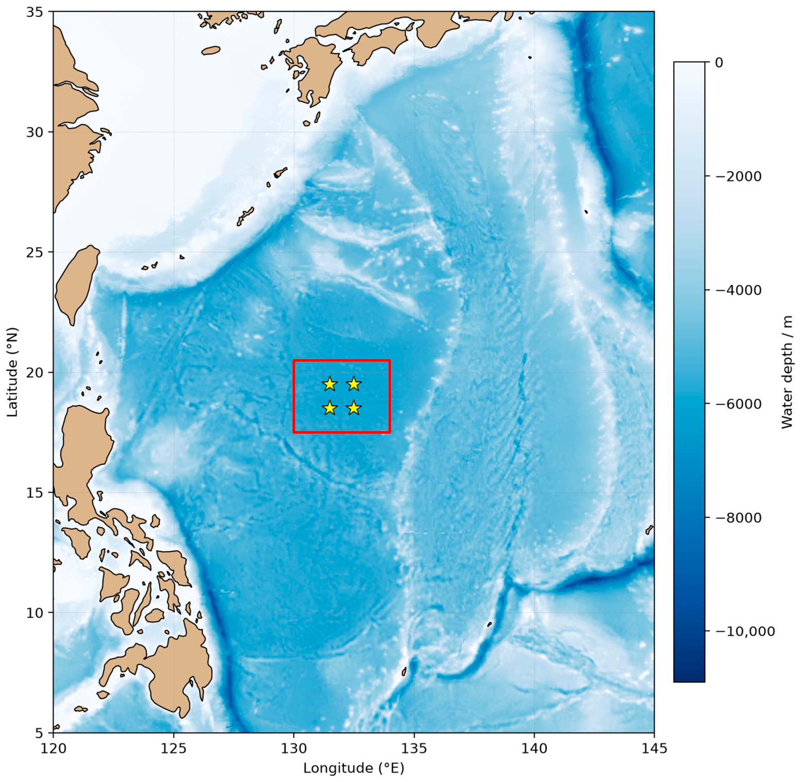
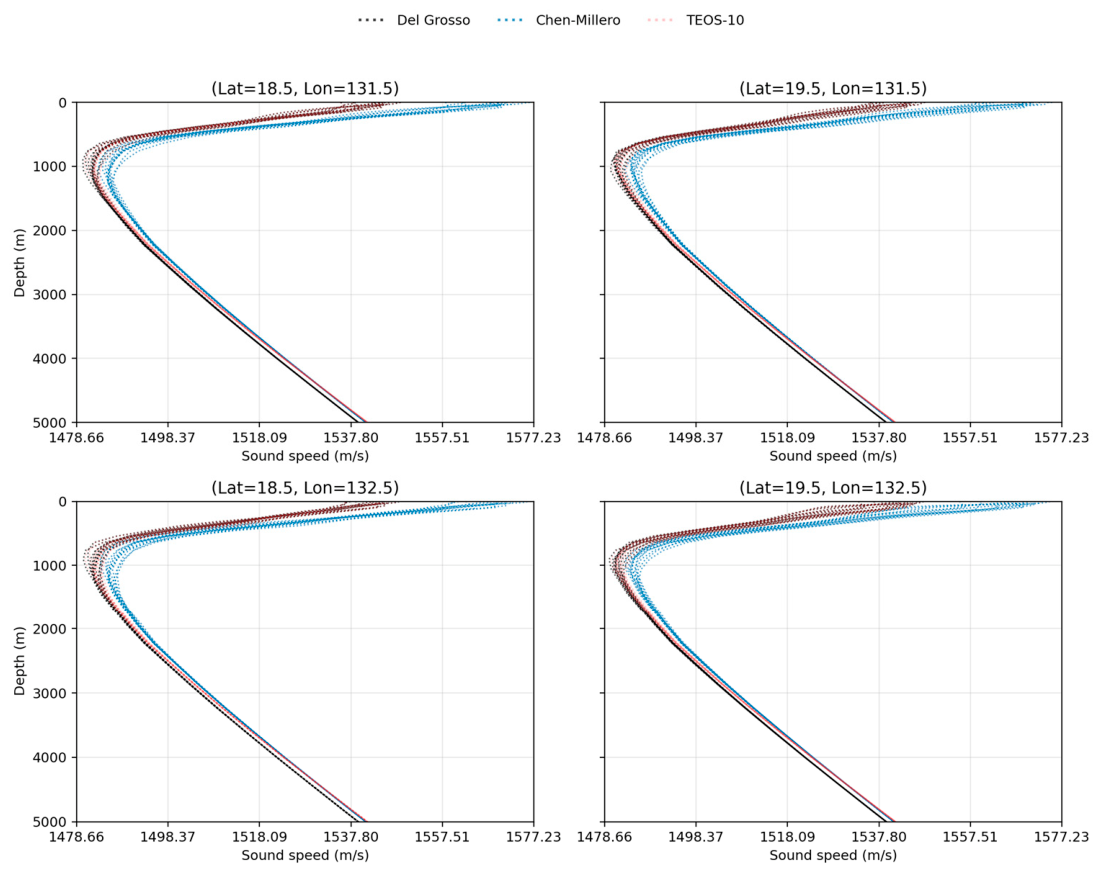
Building on these developments, this study focuses on the central Philippine Basin (130.0–134.0° E, 17.5–20.5° N) and leverages the CMEMS Global Ocean Physics Analysis and Forecast dataset, cross-validated with HYCOM reanalysis data, to systematically investigate the spatiotemporal variations of the sound speed field. The specific objectives are to (1) evaluate the consistency and applicability of CMEMS and HYCOM products in the study region; (2) compare three widely used sound speed formulae (Del Grosso, Chen–Millero, and TEOS-10) and identify the optimal approach for the Philippine Sea; (3) characterize the vertical, horizontal, and temporal variability of the sound speed field through model fitting, gradient analysis, and EOF decomposition; and (4) quantify the seasonal variations of sound channel axis parameters. The results are intended to provide engineering-relevant constraints for underwater acoustic positioning error modeling, AUV mission planning, and deep-sea communication link design in the Philippine Sea region.

2. Data Sources and Processing

2.1. Data Sources

2.1.1. CMEMS Dataset

With the continuous improvement in ocean numerical model resolution, the use of reanalysis and forecast products to study the sound speed field has become an important technical approach. The Global Ocean Physics Analysis and Forecast dataset from the EU Copernicus Marine Environment Monitoring Service (CMEMS) [30] is generated by the Mercator Ocean International operational system. It assimilates multi-source observational data and numerical model outputs, offering high spatiotemporal resolution and accuracy, and has been widely applied in marine acoustics research. This product integrates satellite observations, Argo float profiles, and in situ CTD measurements, containing variables such as temperature, salinity, ocean current, sea surface height, mixed layer depth, and sea ice parameters. Through advanced numerical modeling and data assimilation techniques, high-precision global ocean physical fields are produced. The product has a horizontal grid spacing of 0.083° × 0.083° (approximately 9 km), 50 vertical levels covering 0–5500 m depth, and temporal resolutions supporting hourly, daily, and monthly averages. It has been continuously updated since November 2020.

2.1.2. HYCOM Dataset

HYCOM (Hybrid Coordinate Ocean Model) is a global ocean forecasting system operated by the U.S. Navy. The ESPC-D-V02 dataset employs a hybrid vertical coordinate system that adaptively selects the vertical coordinate, enabling effective resolution of mesoscale eddies and other ocean dynamic processes [31]. This product achieves a horizontal resolution of 1/12° (approximately 9.2 km), with 40 vertical levels covering 0–5000 m depth, containing salinity, temperature, velocity, and elevation information. Developed by the HYCOM consortium with support from the U.S. NOPP, ONR, and Department of Defense, it has a strong scientific research backing. Liu et al. [32] utilized HYCOM data to replace measured sound speed profiles for GNSS-Acoustic seafloor positioning research, demonstrating that HYCOM-derived sound speed profiles achieve horizontal positioning accuracy with an RMS of 0.002 m and vertical positioning accuracy with an RMS of 0.029 m, proving the application value of model data in deep-sea precision positioning.

Based on the above two numerical models, temperature and salinity field data for the central Philippine Sea Basin (130.0–134.0° E, 17.5–20.5° N) from January to December 2025 were extracted. The study area is outlined by the red box in Figure 1, and four evenly spaced points within the domain (18.5° N, 131.5° E; 19.5° N, 131.5° E; 18.5° N, 132.5° E; 19.5° N, 132.5° E) were chosen as target sites for subsequent time-domain analysis (star symbols in Figure 1). The nearest complete year of data was used to analyze the spatiotemporal variation patterns of ocean sound speed in this region. The high spatiotemporal resolution of CMEMS data can accurately capture short-term fluctuations (such as tidal modulation) and seasonal variations, while the hybrid coordinate system of HYCOM data offers outstanding advantages in simulating the vertical thermohaline structure in deep-ocean regions (within 5500 m). Therefore, the two numerical model datasets can complement each other in terms of features, and their results can be cross-validated.

2.2. Validation of Numerical Model Accuracy

As no ground truth is available to evaluate the accuracy of the numerical models, the two datasets were inter-compared. Temperature and salinity information at different depth intervals were compared at each time point, and the daily RMS of data deviations was calculated and plotted as a time series (Figure 2). The statistics of temperature and salinity data deviations by depth interval are presented in

Table 1. Statistics of temperature and salinity data deviations.

Depth Interval	Temperature Deviations (°C)		Salinity Deviations (ppt)
	Mean	Std. Dev.	Mean	Std. Dev.
Full-ocean-depth	0.616	0.087	0.115	0.053
0–50 m	0.510	0.157	0.174	0.094
50–200 m	1.041	0.176	0.085	0.032
200–400 m	0.668	0.161	0.069	0.013
400–1000 m	0.415	0.076	0.052	0.009
1000–2000 m	0.141	0.037	0.016	0.004
2000–5000 m	0.355	0.010	0.008	0.001

. It can be seen that the deviations between the two datasets are mainly concentrated above 400 m, while in the deeper intervals below 400 m, the temperature deviation statistics are within 0.5 °C, with salinity deviation statistics below 0.05 ppt below 400 m.

Based on the four selected points shown in Figure 1, temperature time series at depths of 50 m, 200 m, 400 m, 1000 m, and 2000 m were extracted from the CMEMS and HYCOM datasets, and the results are plotted in Figure 3. The time series comparison shows that the fluctuation trends of the two datasets are consistent, but the fluctuation amplitude of HYCOM data is significantly larger than that of CMEMS data. Due to the absence of systematic variational assimilation of historical observations in HYCOM, high-frequency fluctuations in the Philippine Sea Basin—a region of active mesoscale eddies—are likely dominated by mesoscale eddy signals (spatial scales of 50–200 km, temporal scales of 10–30 days). Fluctuation amplitudes of high-frequency information in temperature time series at different depths were statistically analyzed (

Table 2. Fluctuation amplitude of high-frequency information in temperature time series at different depths (unit: °C).

Depth	CMEMS	HYCOM	HYCOM-CMEMS
50	0.227	0.323	0.096
200	0.186	0.391	0.206
400	0.103	0.398	0.296
1000	0.019	0.069	0.050
2000	0.005	0.015	0.010

). The fluctuation amplitude decreases with increasing depth: the surface fluctuation of CMEMS is approximately 0.2 °C, while that of HYCOM is approximately 0.4 °C; the deep-ocean fluctuations of both are less than 0.1 °C. The mutual difference in fluctuations is largest at 400 m (approximately 0.3 °C), while the differences at 50 m and 2000 m are both less than 0.1 °C. The above results indicate that CMEMS data are more stable than HYCOM data.

CMEMS is a Copernicus Marine Environment Monitoring Service product based on the NEMO ocean model, whereas HYCOM is an operational U.S. Navy system. Both assimilate along-track altimeter sea-level anomalies, satellite-derived sea surface temperature, sea ice concentration, and in situ hydrographic profiles (Argo, XBT, CTD, and moorings). Validation by Jean-Michel et al. [33] indicates that GLORYS12 exhibits root-mean-square deviations (RMSDs) of 0.45 °C for temperature and 0.10 ppt for salinity during the Argo era (2004–2016). Metzger et al. [34] assessed the global accuracy of HYCOM data, reporting a depth-averaged RMSE of <0.5 °C for temperature in the upper 500 m. Hernandez [35] evaluated HYCOM against CTD observations in the Gulf of Mexico (0–300 m), obtaining depth-averaged RMSEs of 0.465 °C and 0.3 ppt for temperature and salinity, respectively.

To ensure that the CMEMS and HYCOM outputs are representative of the Philippine Sea Basin sound speed field and to independently verify their accuracy, 69 Argo temperature and salinity profiles collected in the study area during 2025 were assembled for validation (Figure 4). The distribution of profile maximum depths is as follows: one profile shallower than 300 m, four profiles between 900 m and 1100 m, sixty-three profiles between 1600 m and 2100 m, and one profile deeper than 5500 m. These Argo profiles were quality-controlled and used as reference values for comparison. The intercomparison procedure comprised three steps: Firstly, the CMEMS and HYCOM fields were temporally interpolated to the exact timestamp of each Argo profile to obtain three-dimensional temperature and salinity fields. Secondly, at the horizontal location of each Argo profile, the corresponding model profiles were extracted by horizontal interpolation from these three-dimensional fields. Thirdly, the high-vertical-resolution Argo data were used to interpolate temperature and salinity values at the standard depth levels of the CMEMS and HYCOM grids, enabling a direct comparison at matching depths.

The resulting deviations in CMEMS and HYCOM temperature and salinity from the Argo reference are shown in Figure 5 and Figure 6. Both models exhibit a consistent bias pattern—larger deviations in the upper layers and smaller deviations at greater depths—though, because the two products employ different vertical level discretization, the comparison depths are not identical between datasets. Quantitatively, the full-depth RMS deviations relative to Argo are 0.443 °C (temperature) and 0.084 ppt (salinity) for CMEMS, and 0.737 °C and 0.148 ppt for HYCOM. These results demonstrate that both CMEMS and HYCOM credibly capture the climatological hydrography of the Philippine Sea Basin, with CMEMS exhibiting superior temperature and salinity accuracy relative to HYCOM. Because of the higher accuracy and greater stability, CMEMS data were adopted as the primary data source for sound speed field analysis in this study.

3. Sound Speed Calculation Methods and Comparison

3.1. Traditional Empirical Sound Speed Formulae

In marine acoustics research, traditional empirical sound speed formulae are widely used. They represent statistical summaries of the relationships among temperature, salinity, depth, and sound speed in the ocean. By collecting in situ measurements of seawater temperature, salinity, and sound speed from different ocean regions and depths, the coefficients in these formulae are fitted using multiple regression analysis. In practical applications, ocean temperature and salinity field data are simply substituted into the formula, combined with the corresponding depth information, to rapidly calculate seawater sound speed. This method is computationally simple and fast, offering high practical value for research scenarios where computational efficiency is prioritized and extreme sound speed accuracy is not critical. Currently, the main empirical sound speed formulae fall into two categories: the Del Grosso formula and its derivatives, and the Chen–Millero formula and its derivatives. In addition, the Wilson empirical formula, once mainstream, has been abandoned due to errors in its reference temperature and pressure data.

In 1974, Del Grosso derived the following empirical sound speed formula based on highly reliable experimental data [10]:

$$C=C_{000}+\Delta C_T+\Delta C_S+\Delta C_P+\Delta C_{STP}$$

(1)

where $C_{000}$ is the reference sound speed; $\Delta C_T$, $\Delta C_S$ and $\Delta C_P$ are the correction terms for sound speed changes due to temperature, salinity, and pressure, respectively; and $\Delta C_{STP}$ is the temperature–salinity–pressure coupling correction term. Here, the units of temperature, salinity, and pressure are degrees Celsius (IPTS-68), ppt, and kg/cm², respectively. The Del Grosso formula is relatively accurate among empirical sound speed formulae, but it has strict requirements on the applicable temperature and salinity ranges: temperature 0–30 °C, salinity 30–40 ppt, and pressure 0–1000 kg/cm².

In 1977, Chen and Millero proposed an empirical sound speed formula with a wider applicable range [12]. It is also the UNESCO-recommended UNESCO formula [36]:

$$C=\left(AS+B{S}^{3/2}+C{S}^2\right)+\left(C^0-C_{H_{2}O}^0\right)+C_{H_{2}O}^P$$

(2)

where $A,B,C$ is temperature–pressure-dependent coefficient; $S$ is salinity in ppt; $C^0$ is seawater sound speed at reference pressure (typically one standard atmosphere, i.e., the sea surface); $C_{H_{2}O}^0$ is sound speed of pure water at reference pressure (1 standard atmosphere); $C_{H_{2}O}^P$ is sound speed of pure water at pressure P. The Chen–Millero formula has a wider applicable range than the Del Grosso formula: temperature 0–40 °C, salinity 5–40 ppt, and pressure 0–1000 kg/cm².

3.2. TEOS-10-Based Sound Speed Calculation

The Thermodynamic Equation of Seawater—2010 (TEOS-10) provides a more scientifically rigorous and precise theoretical framework for calculating seawater sound speed [13]. Its core is the use of the Gibbs function as a unified theoretical foundation. Through three independent variables—absolute salinity, conservative temperature, and pressure —it describes all thermodynamic properties of seawater, including density, entropy, and sound speed, avoiding potential inconsistencies among properties that may exist in traditional empirical formulae. The Gibbs function is expressed as

$$g(S_A,\Theta ,p)=g^0(\Theta ,p)+g^{\mathrm{ex}}(S_A,\Theta ,p)$$

(3)

where $g^0$ is the Gibbs function for pure water, calculated accurately through international fluid equations (such as IAPWS-95), and $g^{\mathrm{ex}}$ is the excess Gibbs function for salts, fitted from experimental data to describe the deviation of actual seawater from the ideal state.

Sound speed is the velocity at which acoustic waves propagate in seawater. Its physical essence is directly related to the adiabatic compressibility of seawater and can be determined jointly by seawater density and the adiabatic compressibility coefficient $K_a$. Here, $\rho$ can be obtained from the first-order partial derivative of the Gibbs function with respect to pressure, and $K_a$ from the second-order partial derivative. Consequently, the final explicit sound speed formula is

$$c=\sqrt{{\displaystyle \frac{1}{\rho K_a}}}=\sqrt{{\displaystyle \frac{1}{{\left(\frac{{\partial }^{2}g}{\partial p^2}\right)}_{S_A,\Theta }}}}=\sqrt{{\left({\displaystyle \frac{\partial p}{\partial \rho }}\right)}_s}$$

(4)

where $\rho$ is seawater density, and $s$ represents salinity (absolute salinity $s_A$ in TEOS-10). Through complex mathematical operations on the Gibbs function $g(S_A,\Theta ,p)$, the relationship between density $\rho$ and absolute salinity $s$, conservative temperature $\Theta$, and pressure $p$ is obtained, from which ${\left({\displaystyle \frac{\partial p}{\partial \rho }}\right)}_s$ is derived, ultimately yielding the sound speed.

The calculation principle of TEOS-10 is based on rigorous thermodynamic theory, accounting for the complexity of seawater composition and the nonlinear relationships among thermophysical quantities. Through unified physical quantities and equations of state, it ensures consistency among different thermodynamic properties, avoiding contradictions and errors that may exist in traditional empirical formulae. When calculating seawater sound speed, it can more accurately reflect the combined effects of temperature, salinity, and pressure on sound speed, making it particularly suitable for scientific research requiring high sound speed accuracy.

3.3. Comparison of Sound Speed Calculation Methods

Sound speed profiles at four typical locations were calculated using the mid-month data from the CMEMS dataset for comparison (Figure 7). In the upper layer (0–1000 m), the Chen–Millero (CM) formula yields overall higher sound speed values, with obvious systematic deviations from both the Del Grosso (DG) formula and TEOS-10. In the deep layer below 2000 m, the three methods gradually converge, with TEOS-10 and CM fitting more closely, while systematic deviations between TEOS-10 and DG remain evident. TEOS-10 generally lies between DG and CM in most months, with smoother curves and more natural seasonal variation attenuation with depth. As TEOS-10 is based on the thermodynamic equation of state for seawater, its calculation process more closely approximates the true state of seawater. In contrast, DG and CM are empirical polynomials with more limited applicable ranges and state variable definitions, making them prone to systematic biases. Therefore, this study recommends using the TEOS-10 method for sound speed field calculation in subsequent analyses.

To quantify the systematic deviations among the three methods, we computed the RMS differences among the three sound speed equations at each of the four representative locations across all 12 months (

Table 3. RMS Differences among three sound speed equations at different depths (m/s).

Depth	TEOS vs. Del Grosso	TEOS vs. Chen–Millero	Del Grosso vs. Chen–Millero
50 m	0.075	24.207	24.132
200 m	0.057	17.953	18.010
1000 m	0.386	3.338	3.724
2000 m	0.688	1.530	2.217
3000 m	1.044	0.777	1.821
4000 m	1.467	0.217	1.684

). Del Grosso agrees closely with TEOS-10, with RMSD values of 0.075 m/s at 50 m, 0.057 m/s at 200 m, and 0.386 m/s at 1000 m; even at 4000 m the RMSD is only 1.467 m/s. By contrast, Chen–Millero exhibits much larger deviations from TEOS-10: RMSD reaches 24.207 m/s at 50 m, 17.953 m/s at 200 m, and 3.338 m/s at 1000 m, then decreases to 0.777 m/s at 3000 m and 0.217 m/s at 4000 m. Assuming comparable uncertainties in the two variables used to compute each RMSD, the error magnitude of each variable can be estimated via error propagation as RMSD/√2. Because each method participates in two pairwise comparisons, we averaged the two independent uncertainty estimates for each method to obtain its precision metric, thereby enabling cross-method comparison. TEOS-10 achieves the highest precision at all depths: 8.585 m/s at 50 m, 6.368 m/s at 200 m, 1.317 m/s at 1000 m, 0.784 m/s at 2000 m, 0.644 m/s at 3000 m, and 0.595 m/s at 4000 m. Del Grosso shows significantly better precision than Chen–Millero at 50 m (8.558 vs. 17.090 m/s), 200 m (6.388 vs. 12.715 m/s), and 1000 m (1.453 vs. 2.497 m/s). At 2000 m, the two methods converge to comparable precision (1.027 vs. 1.325 m/s). Conversely, Chen–Millero surpasses Del Grosso at greater depths: 0.919 vs. 1.013 m/s at 3000 m, and 0.672 vs. 1.114 m/s at 4000 m. This superior performance of TEOS-10 is attributable to its Gibbs-function formulation, which inherently satisfies the Maxwell relations among thermodynamic properties [13], thereby eliminating the systematic biases that arise from independently fitted polynomials in the Del Grosso and Chen–Millero approaches. For the Philippine Basin, where the water column spans 0–5500 m and temperature ranges from 28 °C at the surface to 1.5 °C at the seafloor, TEOS-10’s self-consistent thermodynamic framework minimizes extrapolation errors and is therefore adopted as the reference method for all subsequent analyses.

4. Analysis of Sound Speed Field Variations

4.1. Vertical Variation of Sound Speed

To analyze the vertical variation patterns of sound speed in the study area, the sound speed field data generated from the CMEMS dataset were first read. For January–December 2025, all temporal samples within each month were extracted, and spatial and temporal averaging was performed over the full horizontal range (all longitude–latitude grid points) at each depth level to obtain a representative monthly mean sound speed profile for that month. To reduce the influence of area differences among latitude grid cells on the spherical coordinate system, the horizontal averaging employed area-weighting (using the cosine of latitude as the weight), yielding a more physically representative domain-averaged profile. The profile depth range was standardized to 0–5000 m. After obtaining the monthly mean profiles, each month’s sound speed profile was fitted using three vertical structure models: the bi-exponential model [37], the Munk canonical sound speed profile model [22], and the polynomial model.

(1)

Bi-exponential model: A constrained nonlinear least-squares fitting of a bi-exponential vertical model was performed to obtain parameters and compute the fitted sound speed:

$$c(z)=c_{\infty }+a_1{e}^{-z/h_1}+a_2{e}^{-z/h_2}$$

(5)

where $c_{\infty }$ is the deep-ocean asymptotic sound speed, representing the intrinsic sound speed level of deep-water masses, independent of surface-layer thermal variations. $a_1$ and $a_2$ are amplitude coefficients; $h_1$ and $h_2$ are decay scale parameters. The two exponential terms describe the deviations from this baseline in the upper water column. The first term captures the upper-water-column (50–600 m) deviations, reflecting the thermally dominated stratification of the upper ocean, while the second term describes the intermediate and deep stratification (600–2000 m), corresponding to water-mass formation and interior boundary mixing processes in the lower ocean. Zhu et al. [37] independently validated the bi-exponential parameterization using GNSS-Acoustic observations, demonstrating that the model accurately captures the two-layer thermocline structure.

(2)

Munk canonical sound speed profile model: The classical Munk profile model parameters were fitted through nonlinear least squares to obtain parameters and compute the fitted sound speed:

$$c(z)=c_0\left[1+\epsilon \left(\eta +e^{-\eta }-1\right)\right],\eta ={\displaystyle \frac{z-z_0}{B}}$$

(6)

where $z_0$ is the sound channel axis depth; $c_0$ is the sound speed at the channel axis; $B$ is the sound channel thickness scale parameter; and $\epsilon$ is the perturbation parameter. Chen et al. [38] proposed that Munk canonical sound speed profile model could be used to invert the time-varying ocean sound velocity profile model, thereby providing positioning services for underwater vehicles.

(3)

Polynomial model: A least-squares polynomial regression between depth and sound speed was performed for each profile. In alignment with the parameter count of the bi-exponential model, a polynomial of order 4 was specified. The coefficients thus obtained were employed to compute the fitted sound speed:

$$c(z)={\displaystyle \sum _{k=0}^n{a}_k}{z}^k$$

(7)

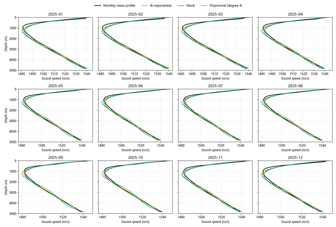
The “monthly mean sound speed profile vs. model-fitted curve” results for the 12 months were compared and analyzed (Figure 8). Each subplot corresponds to one month, with the black solid line representing the monthly mean sound speed profile and the fitted curves of the three models superimposed. The fitting results show that all three fitting methods yield overall structures consistent with the mean sound speed profile. However, the polynomial fitting exhibits physically unrealistic fluctuations in the deep-ocean region, while the bi-exponential model follows the reference profile more closely. 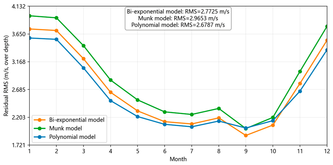The RMS fitting error statistics for each model were computed (Figure 9): the polynomial method has the smallest residual (2.68 m/s), the bi-exponential model ranks second (2.77 m/s), and the Munk model has the largest residual (2.97 m/s). The RMS difference between the polynomial method and the bi-exponential model is only 0.09 m/s (approximately 3% of the polynomial residual), which means the polynomial model does not offer statistically superior performance comparing to the bi-exponential model. The correlation coefficients of parameters within the same model and between different months were also statistically analyzed (

Table 4. Correlation statistics of model parameters.

Model Type	Intra-Model	Inter-Month
Bi-exponential Model	0.878	0.857
Munk Model	0.782	0.696
Polynomial Model	0.887	0.898

). The inter-month correlation of bi-exponential parameters (0.857) is comparable to that of the polynomial model (0.898), and the intra-model correlation (0.878) is also close to the polynomial model (0.887). These correlations are markedly stronger than those computed from the Munk model.

The bi-exponential model decomposes the vertical sound speed profile into two physically distinct layers that map explicitly onto the stratification structure of the Philippine Sea basin. The first exponential term corresponds to the main thermocline (50–400 m) and upper pycnocline (400–600 m), where the characteristic scale reflects the e-folding depth of temperature gradient decay within this layer. In the tropical–subtropical northwestern Pacific, this permanent thermocline is controlled by wind-driven Ekman pumping and eddy–mean flow interaction; the second exponential term corresponds to the intermediate and deep stratification (600–2000 m), with its larger characteristic scale (slower decay) reflecting the weak temperature gradient structure of deep-water masses such as North Pacific Intermediate Water (NPIW) and Deep Water (NPDW). Meanwhile, it naturally converges to a constant asymptotic sound speed (c∞) at depth, which is physically consistent with the oceanographic reality. In contrast, the polynomial coefficients (a₀ through a₄) have no direct physical meaning—they are purely mathematical fitting parameters that cannot be linked to ocean dynamic processes. Additionally, the polynomial model exhibits physically unrealistic oscillations in the deep ocean (below 2000 m), where the fitted curve deviates from the monotonic sound speed increase expected from adiabatic compression. This is a well-known artifact of high-order polynomial extrapolation beyond the fitted domain.

Although the polynomial model performs marginally better across the metrics, its lack of physical interpretability and poor performance in deep-ocean regions limit its practical applicability. The Munk model has certain physical meaning that describes the canonical sound speed profile, but its relative metrics in this area show the poorest performance, which means the poorest generalizability. The bi-exponential model exhibits comparable performance to the polynomial model, and its parameters (c∞, A₁, A₂, k₁, k₂) can be directly used to construct empirical sound speed profile templates for GNSS-Acoustic positioning and AUV navigation. Therefore, considering the balance between statistical fitting accuracy and physical interpretability, the bi-exponential model is recommended as the choice for characterizing vertical sound speed variations in this region.

4.2. Horizontal Variation of Sound Speed

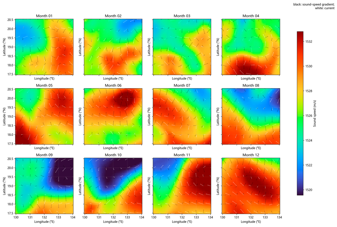
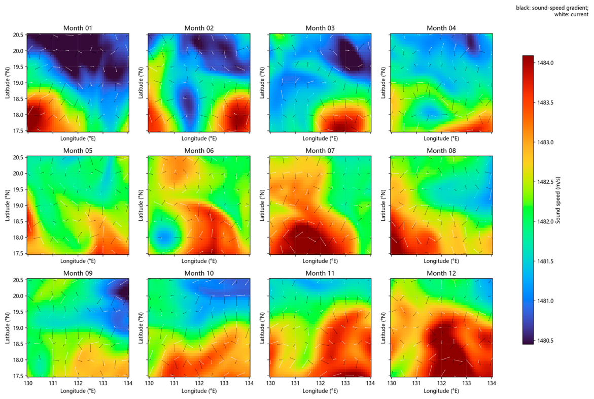
To analyze the horizontal variation patterns of sound speed in the study area, the sound speed field data and ocean current data generated from the CMEMS dataset were retrieved. Sound speed sections and ocean current sections at depths of 200 m and 1000 m were extracted. At 200 m—near the upper boundary of the permanent thermocline where the vertical temperature gradient is steep—mesoscale eddy-induced isopycnal displacements generate large thermohaline anomalies through gradient amplification. Consequently, this depth exhibits the most pronounced horizontal sound speed variability associated with eddy-induced thermohaline perturbations. Additionally, 1000 m corresponds to the typical sound channel axis depth range in the central Philippine Basin (as confirmed in Section 4.4), representing the region of minimum sound speed where long-range acoustic propagation is most sensitive to horizontal gradients. Together, these levels bracket the thermocline-to-SOFAR transition, enabling a comprehensive characterization of the mechanisms controlling lateral sound speed variability from the upper thermocline to the sound channel.

For January–December 2025, temporal averaging was performed on the sound speed and ocean current sections for each month to obtain representative monthly mean sound speed sections and monthly mean ocean current sections. To analyze the horizontal variation patterns, horizontal gradients were computed and compared with ocean current data (Figure 10 and Figure 11). The results reveal a weak direct correlation between the two vectors, yet their directions display a cross-directional pattern. In addition, their magnitudes exhibit concerted variations. Therefore, correlations between the northward sound speed gradient and northward ocean current, and between the eastward sound speed gradient and eastward ocean current, were separately computed (

Table 5. Correlation between sound speed horizontal gradients and ocean current data (same direction).

Month	Depth 200 m		Depth 1000 m
	E. SS Gradient & E. Current	N. SS Gradient & N. Current	E. SS Gradient & E. Current	N. SS Gradient & N. Current
1	0.330	−0.128	−0.250	0.037
2	0.001	0.003	−0.045	−0.027
3	−0.243	0.314	−0.084	0.219
4	−0.040	−0.039	0.040	0.112
5	−0.052	0.187	−0.236	−0.027
6	0.237	−0.193	−0.185	0.184
7	−0.486	0.428	0.080	0.067
8	−0.132	−0.040	0.029	−0.079
9	0.327	−0.400	0.006	−0.214
10	0.432	−0.348	0.278	−0.213
11	0.292	−0.194	−0.116	−0.128
12	−0.345	0.41	−0.024	0.001
Mean Absolute Value	0.243	0.224	0.114	0.109

); correlations between the northward sound speed gradient and eastward ocean current, and between the eastward sound speed gradient and northward ocean current, were also separately computed (

Table 6. Correlation between sound speed horizontal gradients and ocean current data (cross direction).

Month	Depth 200 m		Depth 1000 m
	E. SS Gradient & N. Current	N. SS Gradient & E. Current	E. SS Gradient & N. Current	N. SS Gradient & E. Current
1	−0.462	−0.238	0.529	−0.612
2	−0.109	−0.073	0.747	−0.646
3	0.336	−0.409	0.554	−0.741
4	0.550	−0.692	0.078	−0.442
5	0.571	−0.803	0.497	−0.438
6	0.695	−0.850	0.738	−0.657
7	0.772	−0.784	0.503	−0.492
8	0.838	−0.922	0.440	−0.175
9	0.745	−0.867	0.539	−0.322
10	0.774	−0.634	0.423	−0.415
11	0.783	−0.852	0.145	−0.348
12	0.598	−0.775	0.462	−0.268
Mean Absolute Value	0.603	0.658	0.471	0.463

). The full monthly correlation matrices are provided in Table 5 and Table 6 for reference; the key conclusion is that the cross-directional correlation is significantly stronger than the same-directional correlation. The correlation between sound speed gradients and ocean currents in the same direction is weak, with mean absolute values of 0.114 and 0.109 in the two directions, and maximum values of 0.278 and 0.219, respectively. In contrast, the cross-directional correlation between sound speed gradients and ocean currents is relatively strong, with mean absolute values of 0.471 and 0.463, and maximum values of 0.747 and 0.741, respectively. Considering that horizontal sound speed distribution is governed by thermohaline structure, these results indicate that horizontal flow field-driven changes in thermohaline structure are an important driver of the horizontal sound speed distribution.

The study region (130.0–134.0° E, 17.5–20.5° N) lies on the northern edge of the North Equatorial Current (NEC) bifurcation zone. The NEC transports warm water westward across the Pacific and bifurcates at the Philippine coast into the northward-flowing Kuroshio Current (KC) and the southward-flowing Mindanao Current (MC), with the bifurcation latitude exhibiting strong seasonal variation and depth dependence. Qu and Lukas [39] analyzed historical hydrographic data and showed that the near-surface bifurcation latitude reaches its southernmost position at 14.8° N in July and its northernmost position at about 17.2° N in December. The bifurcation shifts northward with depth, reaching north of 20° N at depths around 1000 m and as far north as 22° N below 700 m during the northeast monsoon (November–January). The northward shift of the deep bifurcation is manifested as the Luzon Undercurrent (LUC)—a southward-flowing intermediate water along the eastern Philippine coast [39]. Observations by Wang et al. [40] indicate that the main body of the NEC is concentrated south of 14° N, and at 18° N along 130° E the mean velocity is only −0.02 m/s with highly variable direction, confirming that 18°N is the northern boundary of the NEC. Therefore, the study region (17.5–20.5° N) is primarily influenced by Kuroshio-origin water rather than by direct NEC advection.

During summer, when stratification intensifies, warm and high-salinity Kuroshio water intrudes into the region, enhancing the thermocline strength and increasing sound speed gradients. During winter, the mixed layer deepens and thermodynamic stratification weakens, causing sound speed gradients to decrease. The correlation coefficient of ~0.5 reflects the combined modulation of sound speed gradients by Kuroshio advection and thermodynamic stratification: the cross-directional correlation between sound speed gradients and horizontal ocean currents captures the advective effect of the Kuroshio and its associated eddy field on the thermohaline structure. In addition to the Kuroshio, mesoscale eddy advection, wind-driven Ekman pumping that modulates thermocline depth, and high-frequency variability generated by baroclinic instability also contribute to sound speed gradient variability in this region. This explains why the correlation is only ~0.5 rather than higher: the Kuroshio provides the background mean advection that sets the seasonal envelope, while eddies and local wind forcing provide the intra-seasonal perturbations. The 1-month lag corresponds to a westward displacement of approximately 80–130 km, consistent with the mesoscale eddy propagation time scale in the subtropical northwestern Pacific.

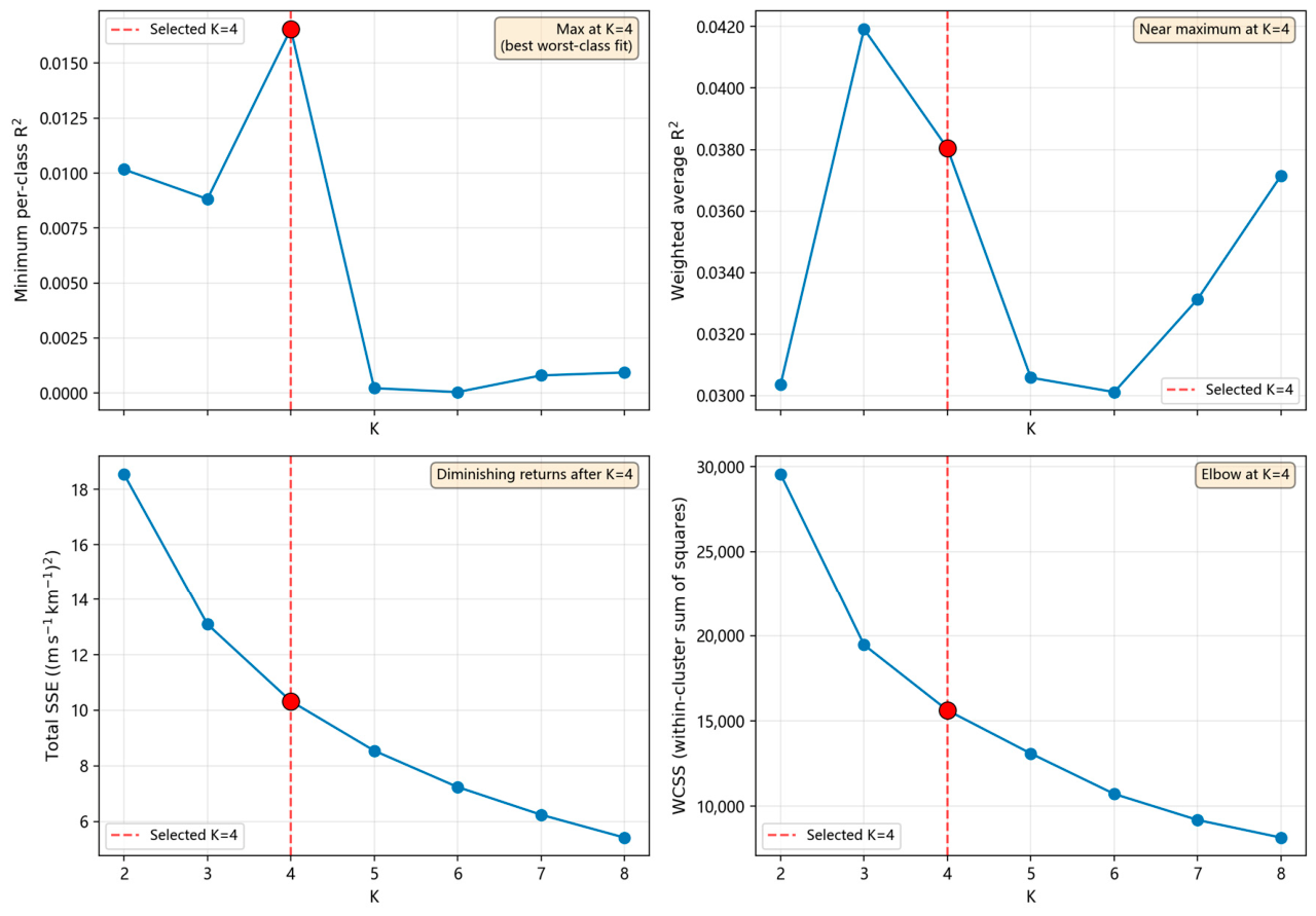
Given that sound speed horizontal gradient values are small and vary slowly, a linear model was considered for approximation within a certain range. Unsupervised classification of horizontal gradients of the sound speed section at 200 m depth was performed, using the linear approximability of north–south and east–west gradients in each class as a constraint condition to determine the number of classes. To determine the optimal number of clusters, K-means clustering was performed for K = 2, 3, …, 8, with both linear approximation capability and clustering structure examined, as shown in Figure 12. When K = 4, the minimum intra-class coefficient of determination (minimum per-class R²) reached its maximum value of 0.0166; that is, the class “most difficult to approximate linearly” exhibited the best goodness of fit under the latitude–longitude linear function. Its overall linear approximation quality (weighted average R²) was 0.0380, second only to the value for K = 3. 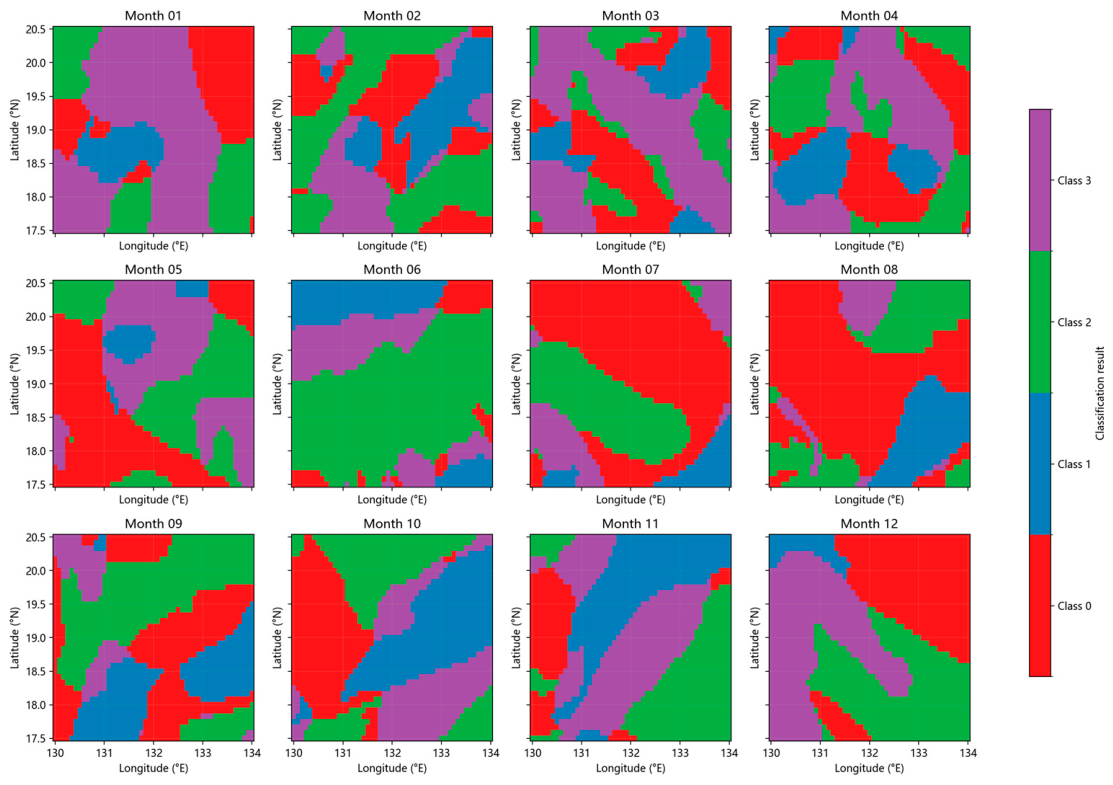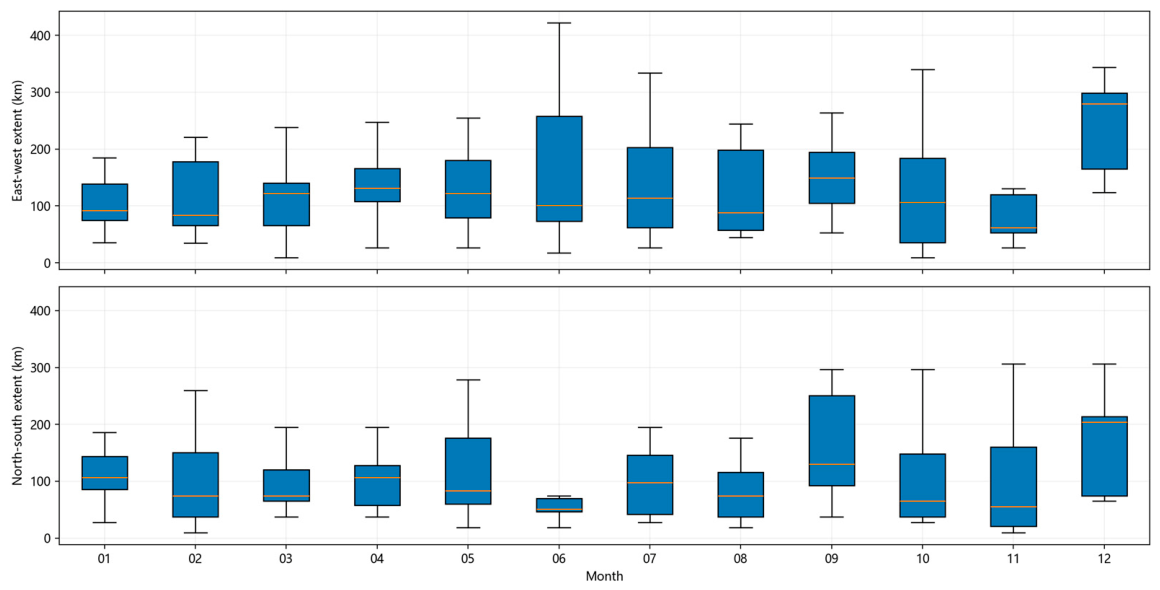In addition, the marginal decrease in the total sum of squared errors (SSE) for line fitting (10.33 m·s⁻¹·km⁻¹) also began to slow markedly from K = 4 onward, and the within-cluster sum of squares (WCSS) showed a distinct elbow point after K = 4. Therefore, considering linear constraints, clustering compactness, and diminishing error returns comprehensively, this study divides the horizontal sound speed gradients in the study area into four classes. Using the K-means method, which minimizes the sum of squared distances from samples to their cluster centers, the unsupervised classification of horizontal gradients at 200 m depth was implemented (Figure 13). Based on the monthly median extent across all connected regions, the control ranges of each region in the classification results were statistically analyzed (Figure 14 and

Table 7. Overall statistical results of unsupervised classification (unit: km).

Statistic	East–West Direction	North–South Direction
Median	120.821	93.540
Maximum	370.030	299.946
Minimum	35.901	27.830
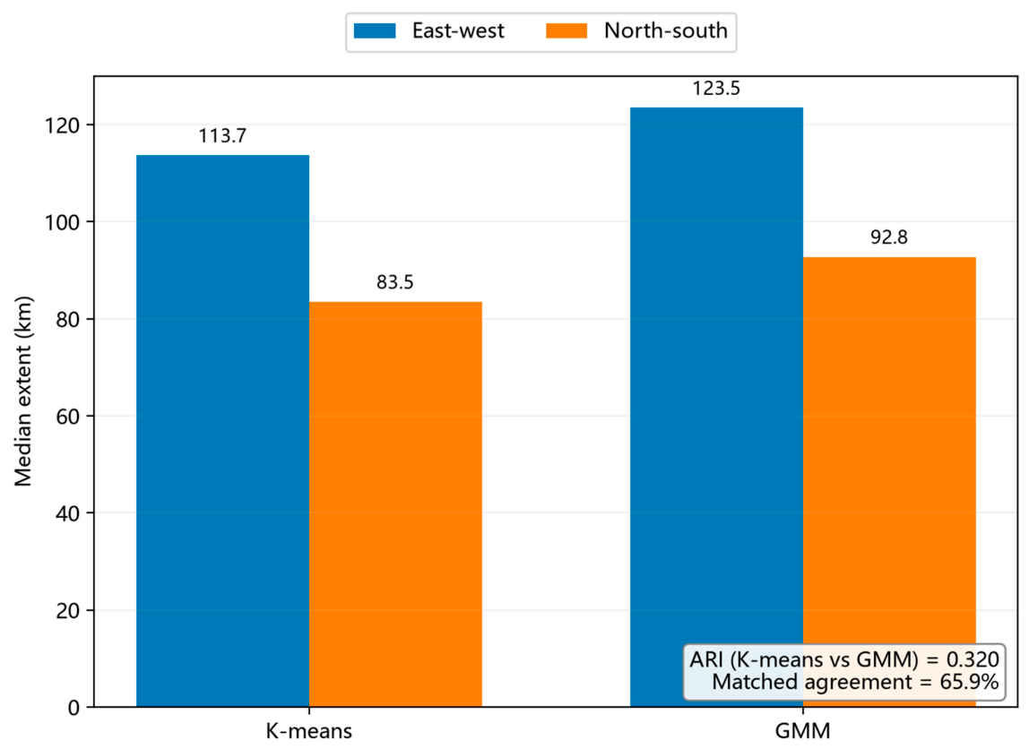
Standard Deviation	99.458	83.1421

). The median coverage ranges of each region in the unsupervised classification results are similar across different months, with the mean east–west coverage range being 120.821 km (minimum 35.901 km) and the mean north–south coverage range being 93.540 km (minimum 27.830 km). To further validate the robustness, based on the median extent across all connected regions throughout the year, we compared K-means results with Gaussian mixture model (GMM) clustering (Figure 15). The GMM produced nearly identical control ranges, and the difference is <1% for both directions. The matched agreement between the K-means and GMM results is 65.9%, indicating that approximately two-thirds of the samples are classified into the same category by both methods. As K-means employs spherical clusters to fit the gradient distribution, whereas GMM adopts elliptical clusters for partitioning, the gradient boundaries delineated by the two methods differ. Accordingly, the adjusted Rand index (ARI) between the two classification results is 0.320, reflecting a moderate similarity in the overall structure. This cross-method consistency confirms that the control range estimate is robust to the choice of clustering algorithm. Therefore, the conservative control range of horizontal gradients within continuous zones can be considered as 30 km × 30 km, and the general control range as 100 km × 100 km. As the horizontal sound speed gradient is estimated in a linear manner in GNSS-Acoustic positioning [41], and its implementation range is less than 10 km × 10 km, the above conclusion indicates that the GNSS-Acoustic method for estimating the horizontal sound speed gradient is appropriate.

4.3. Temporal Variation of Sound Speed

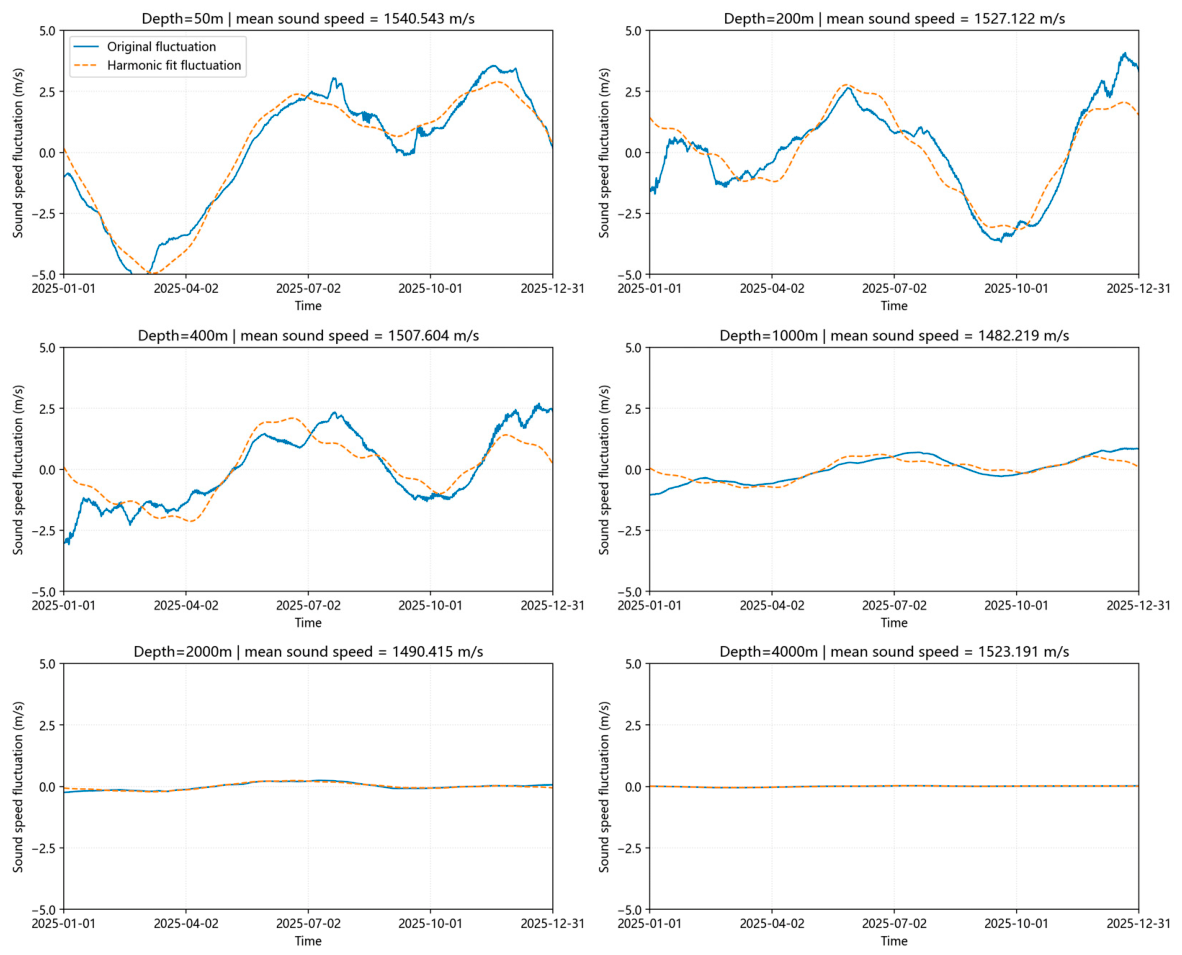
Based on the four-dimensional original sound speed field, for each time step and depth, weighted averaging was performed in the horizontal direction over longitude and latitude (with the cosine of latitude as the weight), compressing the four-dimensional field into two dimensions to obtain a regionally averaged sound speed profile sequence varying with time. From this two-dimensional sequence, sound speed time series at depths of 50 m, 200 m, 400 m, 1000 m, 2000 m, and 4000 m were extracted for temporal modeling and analysis. The original sound speed fluctuations relative to the mean sound speed at different depths are shown in Figure 16, indicating that the peak-to-peak variation of sound speed decreases significantly with increasing depth, from approximately 8.9 m/s fluctuation at 50 m depth to less than 0.1 m/s at 4000 m depth. To quantitatively characterize this multi-scale temporal structure, a harmonic function comprising five frequency components was used to fit the sound speed time series at each depth (Equation (8)). These five components were selected to represent distinct physical forcing mechanisms operating at well-separated time scales:

(1)

The annual cycle (tropical year, 365.2425 days) captures the dominant solar radiative forcing: seasonal insolation variations drive basin-scale changes in sea surface temperature (amplitude ~4 °C) and mixed-layer depth in the Philippine Sea, yielding annual sound speed fluctuations of up to 2.8 m/s at 50 m depth.

(2)

The semi-annual cycle (~180 days) is linked to the biannual equinoxial solar forcing and monsoon transitions in the western Pacific, which generate distinct spring and autumn warming phases in the southern Philippine Sea; additionally, seasonal-to-intra-annual modulation of the NEC bifurcation latitude and Mindanao Current transport may contribute to weaker semi-annual variability in the subsurface thermohaline structure.

(3)

The third harmonic of the annual cycle (~122 days) arises from the asymmetric response of the upper ocean to seasonal forcing: differences in the onset timing of stratification and mixing between the warming and cooling phases produce deviations from a pure sinusoidal annual cycle that are captured by this higher harmonic.

(4)

The quasi-monthly component (~27 days, representative of the tropical month, 27.3 days) is associated with the modulation of mesoscale eddy kinetic energy, possibly linked to baroclinic instability growth rates, as well as to subseasonal atmospheric forcing (e.g., 30–60 day Madden–Julian oscillation and 10–20 day quasi-biweekly variability).

(5)

The daily cycle (1.0 day) resolves the diurnal solar heating and nocturnal cooling effects on the upper-ocean stratification, which are most pronounced in the upper 50 m where the diurnal temperature cycle modulates near-surface sound speed by ~0.01 m/s.

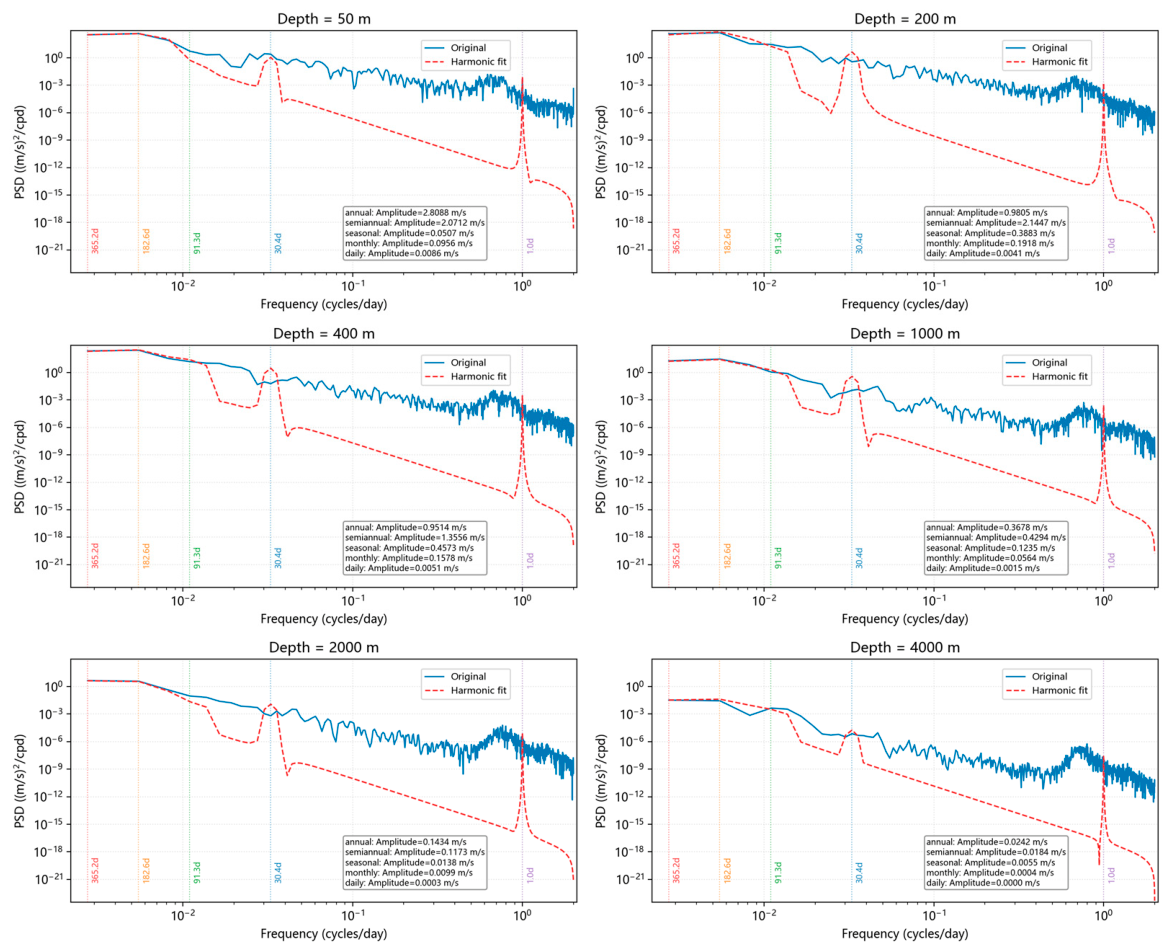
The fitting results in Figure 16 show high agreement between the multi-harmonic model and the original sound speed time series. The power spectral density of the original sound speed data and the harmonic fitting results in Figure 17 consistently exhibit pronounced peaks at the annual and semi-annual periods. The amplitudes of different periodic components shown in Figure 17 were statistically computed using Equation (9). Those results demonstrate that the annual and semi-annual cycles are the dominant components. The annual cycle reaches its maximum amplitude at 50 m (2.81 m/s), accounting for 61.97% of the variance there, while the semi-annual cycle peaks at 200 m (2.14 m/s) and explains 65.08% of the variance at that depth. The combined annual plus semi-annual contribution exceeds 95% at 50 m, is about 78.7% at 200 m, is 63–64% between 400 and 1000 m, and rises back to approximately 90% below 1000 m because the residual variance becomes very small. This vertical pattern is consistent with the physical expectation that solar radiation and monsoon forcing primarily affect the upper ocean, while the deep layer retains a strong large-period signal with small absolute amplitudes.

$$\begin{array}{l}y(t)=a_0+a_{\mathrm{yr}}\cos \left(2\pi t/365.2425\right)+b_{\mathrm{yr}}\sin \left(2\pi t/365.2425\right)+\\ a_{\mathrm{hy}}\cos \left(2\pi t/182.62125\right)+b_{\mathrm{hy}}\sin \left(2\pi t/182.62125\right)+\\ a_{\mathrm{se}}\cos \left(2\pi t/91.310625\right)+b_{\mathrm{se}}\sin \left(2\pi t/91.310625\right)+\\ a_{\mathrm{mo}}\cos \left(2\pi t/30.436875\right)+b_{\mathrm{mo}}\sin \left(2\pi t/30.436875\right)+\\ a_{\mathrm{dy}}\cos \left(2\pi t/1.0\right)+b_{\mathrm{dy}}\sin \left(2\pi t/1.0\right)\end{array}$$

(8)

$$A_k=sqrt(a_k^2+b_k^2)$$

(9)

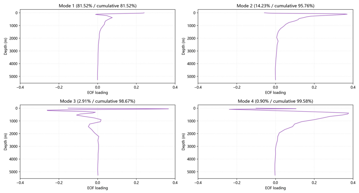
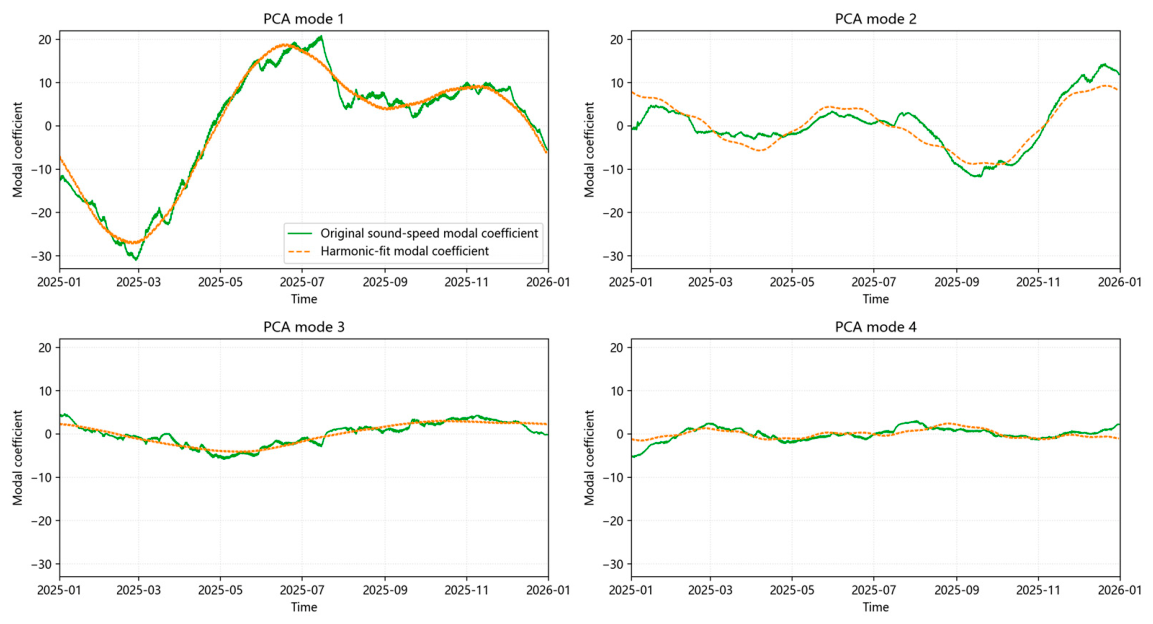
Sound speed at different depths exhibits completely different temporal variation patterns. To facilitate temporal modeling of sound speed, empirical orthogonal function (EOF) analysis was performed on the sound speed profile time series. Modes with cumulative variance contribution exceeding 99% were retained, and mode profiles (Figure 18) and modal coefficient time series (Figure 19) were output. The mode profiles express the vertical structural shapes corresponding to the dominant modes, while the modal coefficient time series indicate the temporal intensity variations of the primary profile changes. EOF analysis results show that the first four modes already achieve an information contribution rate of 99.58%, with the first two modes alone reaching 95.76%. Harmonic functions were used to temporally fit the modal coefficient time series. The harmonic amplitudes of annual, semi-annual, seasonal, monthly, and daily cycles are presented in

Table 8. Amplitudes of periodic signals in harmonic fitting of modal coefficients (unit: m/s).

Mode	Annual Periodicity	Semi-Annual Periodicity	Seasonal Periodicity	Monthly Periodicity	Daily Periodicity
1	16.094	11.079	0.429	0.203	0.346
2	3.521	6.450	1.212	0.523	0.078
3	3.429	0.558	0.187	0.029	0.148
4	0.599	0.899	0.813	0.250	0.113

. The harmonic fitting results show that annual and semi-annual cycles are the dominant signals in the first three modes, while semi-annual and seasonal cycles are the main components in the fourth mode. These results can effectively fit the temporal variation patterns of sound speed in this sea area.

4.4. Variation of Sound Channel Axis Parameters

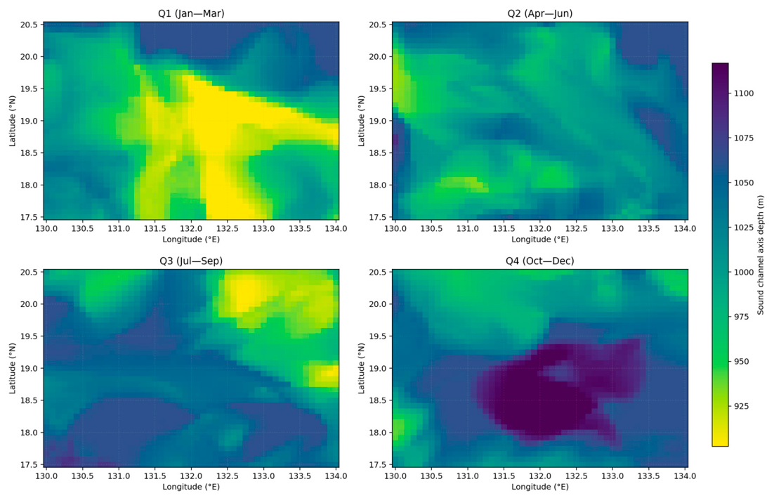
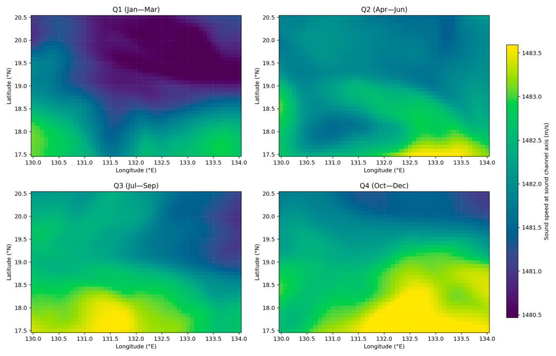
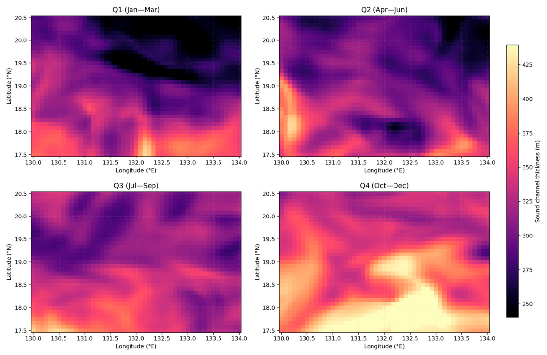
Based on the four-dimensional sound speed field, vertical sound speed profiles were extracted at each time step and horizontal grid point, and sound channel axis parameters were computed. First, piecewise polynomial fitting was applied to the discrete sound speed profiles for densification. Then, the minimum points on the fitted curve were found, corresponding to the sound channel axis depth. Finally, using a threshold of 0.5 m/s, the upper and lower boundary depths of the sound channel axis were found on the fitted curve, with their difference representing the sound channel axis thickness. To better illustrate the intra-annual variation of the sound channel axis, the time series was divided into four quarters by month (Q1: January–March, Q2: April–June, Q3: July–September, Q4: October–December). Temporal averaging of the sound channel axis depth, sound channel axis sound speed, and sound channel axis thickness at all horizontal positions and time steps within each quarter was performed to obtain quarterly two-dimensional spatial distribution fields (Figure 20, Figure 21 and Figure 22). The statistical results show that the sound channel axis depth varies within the range of 900–1125 m, being deeper in winter and shallower in spring; 1000 m can be used as the prior constraint for the sound channel axis depth in this region. The sound speed at the sound channel axis is relatively stable, varying between 1480 and 1484 m/s (slightly higher in winter and slightly lower in spring). The sound channel axis thickness fluctuates between 225 and 450 m, with a variation range similar to that of the axis depth, being wider in winter and narrower in spring.

Seasonal variations in the depth of the sound channel axis (shallower in summer, deeper in winter, with an amplitude of approximately 40–80 m) are fundamentally driven by the seasonal thermodynamic cycle of the mixed layer depth, and are transmitted downward through the coupling between the thermocline and the sound channel axis. In the study area (the central Philippine Sea Basin), strong wind-driven mixing and surface heat loss in winter deepen the mixed layer, whereas enhanced stratification in summer shallows it. Changes in the mixed layer directly alter the heat capacity distribution in the upper ocean, which in turn modifies the depth of the thermocline, and ultimately changes the depth of the sound speed minimum below the main thermocline—that is, the depth of the sound channel axis.

According to the characteristics of the sound channel axis, the propagation distance of acoustic signals at the sound channel axis depth is much longer than that at depths outside the sound channel axis. However, variations in the depth of the sound channel axis can increase acoustic transmission loss, thereby imposing higher requirements on the transmitted signal intensity of sonar systems. By presetting the source depth, this problem can be circumvented to improve energy efficiency; otherwise, underwater acoustic communication link failures may occur.

Meanwhile, in the process of long-range navigation and positioning, in order to extract high-precision geometric information from the acoustic signal transmission trajectory, it is necessary to estimate the reversal characteristics of the acoustic signals based on the waveguide features. This process is affected by the depth, thickness, and sound speed variations of the sound channel axis. Consequently, the above conclusions can provide a priori constraints for long-range sound channel axis navigation in this sea area, supporting AUV navigation, optimal deployment depths of underwater acoustic nodes, and sonar scientific detection applications.

5. Conclusions

This study investigates the spatiotemporal variability of the three-dimensional sound speed field in the central Philippine Sea (130.0–134.0° E, 17.5–20.5° N) based on one year (2025) of CMEMS and HYCOM ocean reanalysis data, validated against independent Argo profiles. We establish appropriate models to characterize the sound speed calculation formula, vertical structure, horizontal distribution, temporal evolution, and deep-sea sound channel axis variation, and analyze their relationships with regional ocean dynamics. These findings provide a priori marine environmental background constraints for future underwater acoustic navigation and positioning in this region. The main conclusions are as follows:

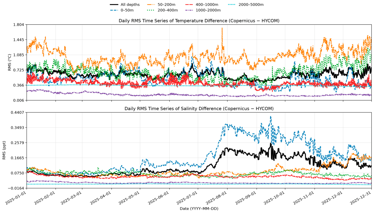
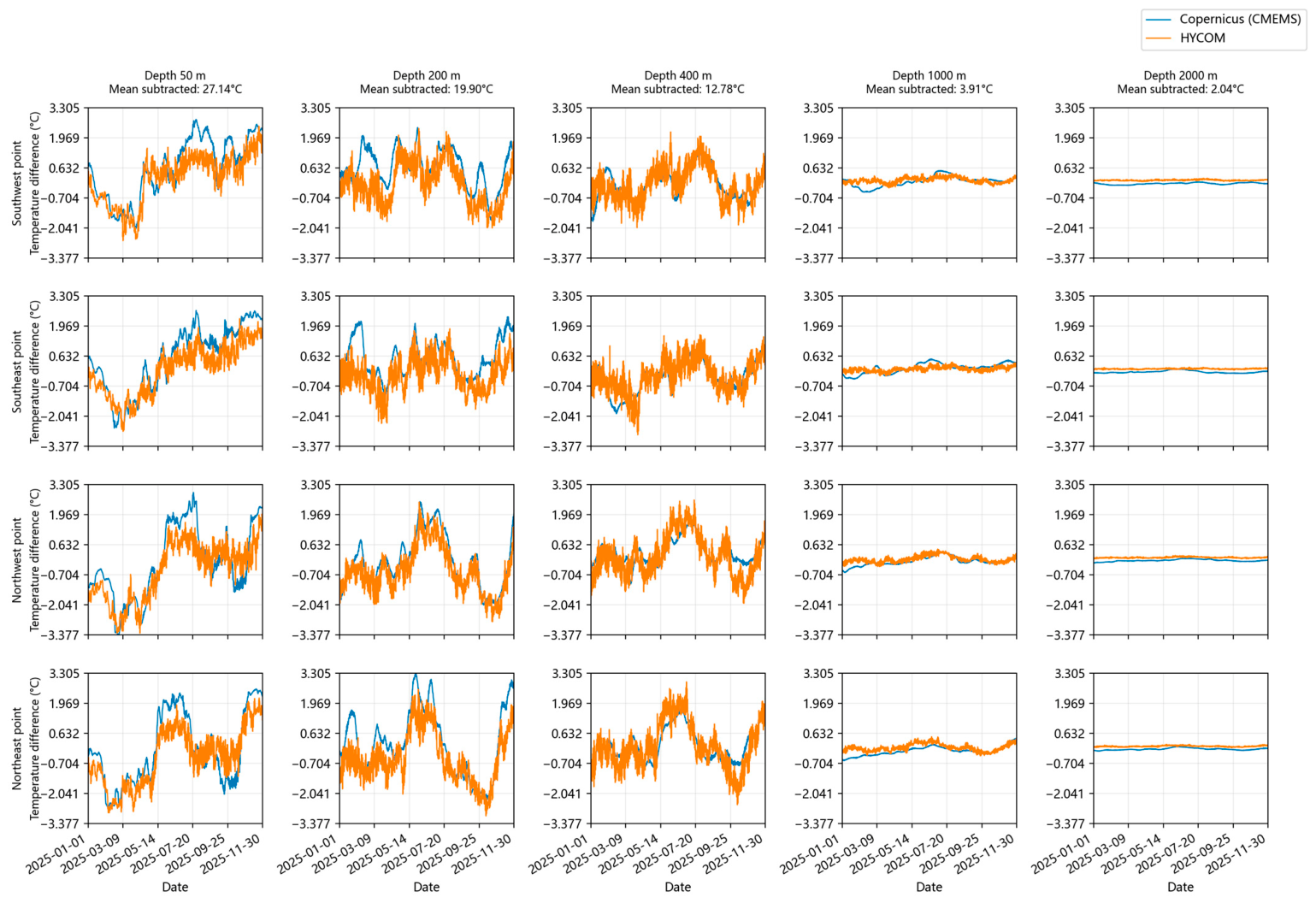
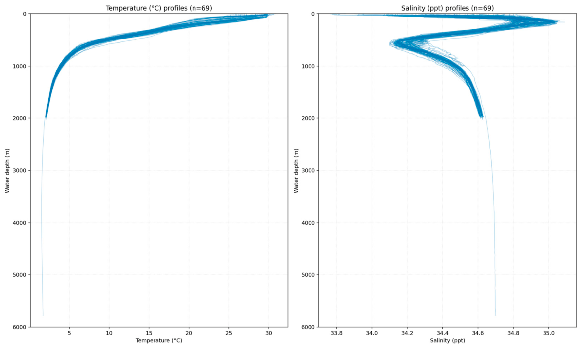
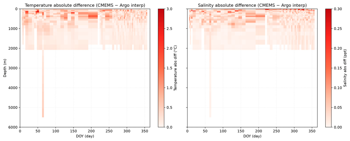
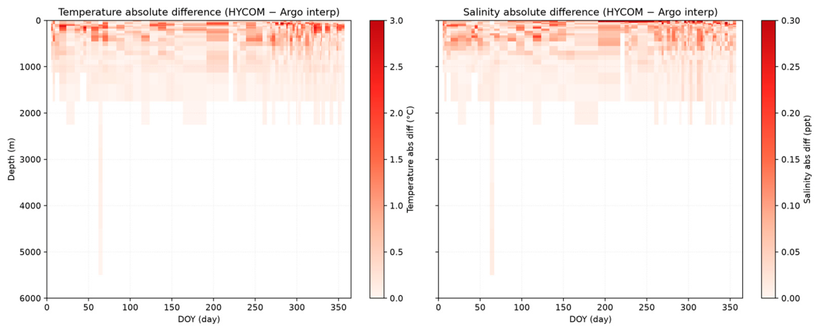
In the study area, the CMEMS and HYCOM datasets exhibit reasonable consistency below 400 m depth, with temperature deviations within 0.5 °C and salinity deviations within 0.05 ppt. However, HYCOM displays significantly greater high-frequency variability than CMEMS. The reliability of the CMEMS representation was independently verified against 69 Argo profiles collected in the study area during 2025, yielding full-depth RMS deviations of 0.443 °C for temperature and 0.084 ppt for salinity—significantly smaller than the corresponding HYCOM deviations (0.737 °C and 0.148 ppt). Considering both stability and accuracy, CMEMS was adopted as the primary data source for subsequent sound speed field analysis. For sound speed computation, the TEOS-10 equation—derived from rigorous thermodynamic principles—outperforms the traditional Del Grosso and Chen–Millero empirical formulae in both physical consistency and computational accuracy of the studied Philippine Basin. These validation steps confirm that the statistical patterns identified in the reanalysis are representative of the actual ocean state and not artifacts of the model formulation.

The vertical structure is best characterized by a bi-exponential parametric model that decomposes the sound speed profile into two physically distinct layers: a fast-decaying term representing the upper-ocean thermocline (50–600 m), controlled by wind-driven Ekman pumping and eddy–mean flow interaction, and a slow-decaying term representing the intermediate and deep stratification (600–2000 m), associated with North Pacific Intermediate Water and Deep Water formation. The model achieves fitting residuals of 2.77 m/s, only 0.09 m/s (approximately 3%) larger than the polynomial model, with comparable parameter stability across months (inter-month correlation 0.857). This marginal difference in statistical performance is outweighed by the physical interpretability of the bi-exponential parameters, which map directly onto the regional stratification structure and naturally converge to a constant asymptotic sound speed at depth.

Regarding horizontal variation, the cross-directional correlation between horizontal sound speed gradients and ocean currents reaches approximately 0.5 in the upper 300 m, reflecting the advective effect of mesoscale eddy stirring in the NEC–Kuroshio bifurcation zone. Anticyclonic eddies elevate isotherms by 50–150 m, producing coherent sound speed increases of 2–6 m/s that propagate westward at typical eddy propagation speeds of 3–5 cm/s. The Kuroshio provides the background mean advection that sets the seasonal envelope of gradient variability, while eddies and local wind forcing supply the intra-seasonal perturbations, explaining why the correlation is approximately 0.5 rather than higher. The spatial control range of horizontal sound speed gradients at 200 m depth is approximately 100 km × 100 km on average, confirmed by cross-validation between K-means and Gaussian mixture model clustering (difference < 1% in both directions).

The temporal sound speed variability decreases significantly with increasing depth, with its peak-to-peak variation decreasing from approximately 8.9 m/s fluctuation at 50 m depth to less than 0.1 m/s at 4000 m depth. The variability can be decomposed into five harmonic components, each corresponding to distinct physical forcing mechanisms: the annual solar radiative cycle (dominant at 50 m depth, explaining 61.97% of the variance), the semi-annual equinoxial and monsoon transition cycle (peaking at 200 m, 65.08%), the asymmetric stratification response to seasonal warming and cooling (~122 days), the quasi-monthly mesoscale eddy kinetic energy modulation (~27 days), and the diurnal solar heating and nocturnal cooling cycle. The combined annual plus semi-annual contribution exceeds 95% at 50 m and approximately 90% below 1000 m, indicating that the deep layer retains a strong large-period signal with small absolute amplitudes. Empirical orthogonal function analysis shows that the first four modes capture 99.58% of the total variance, with the first two modes alone accounting for 95.76%, confirming that the dominant temporal structures are low-dimensional and physically coherent.

The sound channel axis depth undergoes seasonal oscillation between 900 m in summer and 1125 m in winter, with an amplitude of 40–80 m. This variation is fundamentally driven by the mixed layer depth thermodynamic cycle: winter convection entrains cooler subsurface water, weakening the upper thermocline gradient and displacing the sound speed minimum downward, while summer restratification allows the axis to shoal. Concurrently, the sound speed at the channel axis remains stable at 1480–1484 m/s, registering slightly higher values in winter and lower values during the warm season, while the channel axis thickness fluctuates between 225 and 450 m in a “wider in winter, narrower in warm season” pattern. These parameters provide prior oceanographic environment constraints for long-range AUV navigation depth planning, optimal deployment depths of underwater acoustic nodes, and underwater acoustic detection via the sound channel in the study region.

Several limitations point toward future research directions. The CMEMS reanalysis smooths submesoscale and fine-scale thermohaline variability below its effective resolution (~1/12°), which may influence acoustic propagation at higher frequencies and in regions of strong frontal activity. The bi-exponential model parameters, while statistically robust, have not yet been quantitatively linked to specific dynamical scales through process-oriented experiments. The mixed-layer-depth–sound-channel-axis coupling, while physically plausible and consistent with the observed seasonal cycle, should be further tested using one-dimensional mixed-layer models (e.g., the K-profile parameterization) forced with observed surface fluxes to isolate the thermodynamic drivers from advective contributions. Additionally, although the four gradient classes correspond to distinct dynamical regimes in the NEC–Kuroshio bifurcation zone, quantitative attribution of individual classes to specific physical processes remains an unresolved question that warrants dedicated investigation in future work. The harmonic decomposition was focused on seasonal-to-intraseasonal bands; the role of interannual variability associated with ENSO and the Pacific Decadal Oscillation merits dedicated investigation with longer observational records and coupled model output. Nevertheless, the present results establish a systematic, physically grounded framework for understanding sound speed variability in the central Philippine Sea, providing critical constraints for underwater acoustic positioning, AUV navigation, and long-range sound channel communication and navigation in this strategically important region.