Article

Risk-Aware Cooperative Path Planning for Multi-UAV Maritime Offshore Emergency Missions Using a Modified Traffic Jam Optimizer

1
College of Information Engineering, Shanghai Maritime University, Shanghai 201306, China
2
College of Transport & Communications, Shanghai Maritime University, Shanghai 201306, China
3
Engineering Research Center of Integration and Application of Digital Learning Technology, Ministry of Education, Beijing 100039, China
*
Author to whom correspondence should be addressed.
J. Mar. Sci. Eng. 2026, 14(13), 1187; https://doi.org/10.3390/jmse14131187
Submission received: 23 May 2026 / Revised: 23 June 2026 / Accepted: 26 June 2026 / Published: 28 June 2026
(This article belongs to the Section Ocean Engineering)

Abstract

Multi-UAV cooperative path planning is an important technical basis for improving offshore emergency response efficiency in complex maritime environments. However, in complex offshore environments, cooperative trajectory planning is affected not only by geometric obstacles but also by wind disturbances, island terrain, restricted flight zones, and inter-UAV safety and communication constraints. These coupled factors make it difficult for conventional swarm intelligence optimizers to maintain risk awareness, local correction capability, and stable late-stage refinement. To address this problem, this paper proposes a risk-aware Modified Traffic Jam Optimizer for cooperative multi-UAV path planning in complex offshore missions. Unlike the original Traffic Jam Optimizer, the proposed method explicitly incorporates risk information into the population update process. A risk-opposition collaborative guidance strategy is designed to adjust the global search direction away from high-risk regions; a risk-based geometric multiscale adaptive mutation strategy is developed to identify and correct high-risk local control blocks; and a generalized quadratic interpolation decision-vector reconfiguration mechanism is introduced to refine the current best solution during stagnation or late-stage search. Two-UAV and three-UAV simulations are conducted using the constructed offshore environment and cooperative constraint models. The results show that the proposed method can generate feasible cooperative trajectories and achieve better performance than the comparison algorithms in path cost, path length, synchronized flight time, and convergence behavior. These results verify the feasibility and effectiveness of the proposed method for risk-aware multi-UAV cooperative path planning in complex offshore environments.

1. Introduction

Multi-UAV systems have become an important airborne platform for offshore emergency response, marine target monitoring, island-area inspection, and maritime security missions [1,2,3,4]. Compared with a single UAV, multiple UAVs can improve mission efficiency and spatial coverage through task sharing, information exchange, and cooperative flight [2,3,4]. In complex offshore mission scenarios, however, trajectory planning is not only a geometric path-searching problem. It is also a constrained cooperative decision-making problem, in which flight safety, mission execution, and trajectory quality are jointly affected by environmental risks, UAV performance limits, and inter-UAV cooperative constraints [5,6,7,8]. Therefore, generating safe, smooth, and cooperative trajectories under complex offshore constraints is essential for the reliable deployment of multi-UAV systems in maritime missions.
Offshore emergency and maritime monitoring missions often involve UAV trajectory planning under multiple environmental and operational constraints, including marine wind disturbances, island terrain, restricted flight zones, and inter-UAV cooperation requirements [9,10,11]. Compared with general open airspace, offshore mission spaces involve multiple types of constraints, including continuous disturbances, spatial risks, and terrain obstacles. Marine wind fields continuously affect trajectory tracking, flight stability, and energy consumption [12,13]; island terrain restricts the spatial accessibility of candidate trajectories and may introduce terrain-collision risks during low-altitude flight [14,15], restricted fly zones increase mission risks during trajectory traversal, requiring a trade-off between safety and mission efficiency [16,17]. In addition, multi-UAV cooperative flight requires UAVs to maintain appropriate safety and communication distances while coordinating their arrival at the target mission area under speed constraints [7,8]. These coupled factors make offshore multi-UAV path planning not only a practical application problem, but also a representative task for studying risk-aware cooperative path planning in complex marine environments. In this study, “risk-aware” does not refer to a probabilistic risk assessment based on the probability and consequences of an accident. Instead, it means that the planning algorithm explicitly identifies and utilizes deterministic information related to trajectory safety and feasibility. Specifically, terrain clearance, inter-UAV cooperative distance, local trajectory smoothness, and path-structure deviation are transformed into normalized risk-surrogate indicators. These indicators are used to compare the relative risk of local trajectory segments and guide the optimizer toward correcting higher-risk segments. Therefore, the proposed risk indicators support relative risk evaluation and search guidance rather than predicting the actual probability of an accident.
Existing studies on UAV path planning can be broadly categorized into graph-search methods, sampling-based planning methods, mathematical programming methods, and intelligent optimization methods [1,5]. Graph-search methods, such as Dijkstra and A*, can generate interpretable paths in discretized spaces, but their performance strongly depends on grid resolution and may suffer from rapidly increasing search complexity in high-dimensional continuous environments [18,19]. Sampling-based methods, such as RRT and its variants, are effective in finding feasible paths in complex spaces; however, the generated paths often contain redundant turns and require further smoothing and optimization [20,21]. Mathematical programming methods can explicitly formulate constraints, but they may face high computational complexity and limited real-time performance when dealing with nonconvex environments, multiple risk sources, and multi-UAV collaborative constraints [1,5]. In contrast, swarm intelligence optimization algorithms are gradient-free and exhibit strong global search ability and adaptability, making them widely used in complex UAV path planning and engineering optimization problems [22,23].
In recent years, UAV path planning has increasingly been addressed using swarm-intelligence-based optimizers, such as particle swarm optimization, grey wolf optimization, whale optimization, sparrow search algorithms, and other newly developed metaheuristic methods [24,25,26,27]. These methods exhibit promising global search capability in complex nonlinear spaces through population cooperation, stochastic search, and best-solution guidance. However, directly applying general-purpose swarm intelligence algorithms to offshore multi-UAV path planning remains challenging. First, the search directions of many algorithms are mainly driven by individual fitness or global best solutions, without explicit awareness of high-risk regions; this may lead to ineffective searches near terrain obstacles, restricted fly zones, or collaboration-violation regions. Second, path quality is often determined by a small number of local control points, whereas conventional full-vector updates are insufficient for targeted correction of high-risk local segments. Third, in later iterations, the population may prematurely concentrate in local regions, making further refinement of the current best path difficult [23,28]. In addition, existing improved swarm intelligence methods for offshore multi-UAV cooperative path planning have achieved promising results in complex sea-wind environments and collaborative constraint handling [7]; however, their search processes still mainly rely on predefined collaborative control frameworks and population update mechanisms, leaving room for more explicit exploitation of high-risk region distributions and local control-block risks. Therefore, path planning under complex constraints requires an optimization mechanism that can jointly support global risk avoidance, local feasibility correction, and late-stage exploitation.
Traffic Jam Optimizer (TJO) is a recent metaheuristic method whose search behavior is modeled on the process of regulating congested traffic, where candidate solutions are updated through autonomous driving, self-regulation, and traffic-police enforcement phases [29]. Existing studies have shown that TJO has promising search potential in continuous and engineering optimization problems [29]. However, the original TJO is mainly designed for general continuous optimization tasks, and its update mechanism is not explicitly coupled with the risk structure of path planning. When directly applied to offshore multi-UAV path planning, it is difficult for TJO to fully exploit trajectory-related information such as environmental risks, collaborative distances, and path smoothness. In addition, generalized quadratic interpolation (GQI) has been shown to estimate potentially better positions using multiple reference solutions, providing an effective exploitation mechanism for later-stage optimization [30]. Therefore, combining the population search framework of TJO with risk-aware guidance, local geometric correction, and GQI-based refinement is expected to improve its adaptability to path planning under complex constraints. It should be noted that TJO was selected as the baseline optimizer not because it is universally superior to other metaheuristic algorithms, but because its search structure is well suited to the path representation adopted in this study. The control points of multiple UAV trajectories can be directly encoded as high-dimensional continuous decision vectors, which are compatible with the population-based position-update mechanism of TJO. Moreover, its autonomous driving, self-regulation, and enforcement phases provide a gradual transition from global exploration to local exploitation, allowing environmental risks, local path structures, and multi-UAV cooperative constraints to be incorporated into different search stages. Therefore, TJO provides a structurally clear and extensible framework for introducing problem-specific risk guidance, local trajectory correction, and late-stage refinement mechanisms.
Motivated by these challenges, this study introduces a risk-aware Modified Traffic Jam Optimizer (MTJO) to solve cooperative path-planning problems for multiple UAVs in complex offshore environments. Unlike general update mechanisms that mainly rely on historical best information, MTJO explicitly embeds risk information into the population update process, forming a continuous optimization chain involving high-risk region identification, local control-block correction, and late-stage exploitation. Specifically, a risk-opposition collaborative guidance strategy is first designed to correct the global guidance direction using high-risk search regions represented by poorly performing individuals. Then, a risk-based geometric multiscale adaptive mutation strategy is proposed, where path control points are divided into local decision blocks and corrected according to terrain risk, collaborative risk, smoothness risk, and stagnation state. Finally, a GQI decision-vector reconfiguration strategy is introduced to refine the current best solution dimension by dimension using elite reference individuals during stagnation or late-stage search. Through these designs, MTJO improves path-planning performance under complex constraints from the perspectives of global risk avoidance, local feasibility correction, and late-stage exploitation.
The three proposed mechanisms are also fundamentally different from commonly used generic improvement techniques. Conventional opposition-based learning generally generates opposite solutions according to the variable bounds or a reference point without explicitly considering environmental risk distributions or multi-UAV cooperative constraints [31,32]. In contrast, the proposed risk-opposition collaborative guidance strategy identifies high-risk search regions and corrects the overall search direction of TJO. Conventional adaptive mutation mainly adjusts the mutation probability or amplitude according to the iteration number or fitness value, whereas the proposed geometric multiscale adaptive mutation operates on local path-control blocks and simultaneously considers local risk, path geometry, and search stagnation [33,34]. Furthermore, conventional elite learning or local search usually perturbs the current best solution within a predefined neighborhood, whereas the proposed GQI strategy reconstructs the decision vector using multiple high-quality reference solutions and is activated only during stagnation or the late search stage. Therefore, MTJO is not a simple combination of existing opposition-based learning, mutation, and local-search operators. Instead, its three complementary mechanisms are specifically designed for global risk avoidance, local trajectory correction, and late-stage refinement.
The major contributions of this work can be summarized as follows:
  • A risk-aware cooperative path planning problem is formulated for multi-UAV maritime offshore emergency missions, considering wind disturbance, island terrain, restricted flight zones, and inter-UAV safety and communication constraints.
  • A modified Traffic Jam Optimizer is developed for this problem, in which a risk-opposition collaborative guidance strategy is proposed to adjust the population search direction according to high-risk regions.
  • A risk-based geometric multiscale adaptive mutation strategy is designed to improve local trajectory correction by integrating block-level risk evaluation, geometric search directions, and multiscale candidate generation.
  • A GQI-based decision-vector reconfiguration scheme is introduced to enhance late-stage refinement, and the proposed method is evaluated in two-UAV and three-UAV offshore emergency scenarios.
The rest of this paper is arranged as follows. Section 2 describes the offshore environment model, which includes the marine wind field, restricted fly zones, and island terrain. Section 3 introduces the original TJO and the proposed improvement mechanisms of MTJO. Section 4 establishes the flight and cooperative constraints, defines the overall cost evaluation model, and describes the proposed cooperative planning workflow. Section 5 analyzes the simulation results obtained under different offshore scenarios. Section 6 concludes the study and discusses possible directions for future work.

2. Offshore Environment Model

Offshore UAV trajectory generation represents a typical constrained optimization task in complex maritime environments, where trajectory feasibility is jointly affected by external disturbances, spatial risks, and terrain obstacles. Marine wind fields continuously influence flight stability and energy consumption, restricted fly zones determine the risk distribution along candidate trajectories, and island terrain directly constrains the accessible space for safe flight. Therefore, to make the planned paths consistent with offshore mission environments, these factors should be modeled within a unified three-dimensional space. In this paper, the offshore mission space is modeled in three dimensions using a Cartesian coordinate framework, incorporating the wind field, restricted flight regions, and island terrain. Figure 1 illustrates the constructed environment, and the detailed models are described as follows.

2.1. Wind Field

In offshore environments, wind is an important external disturbance affecting UAV path planning. It influences trajectory tracking, flight stability, and energy consumption, and should therefore be considered during planning [12,13]. The Lamb-Oseen function is used to model the local vortex wind field [14], as shown in Equation (1):
V x r d = λ · y y 0 2 π r d r d ¯ · 1 e r d r d ¯ / ζ 2 V y r d = λ · x x 0 2 π r d r d ¯ · 1 e r d r d ¯ / ζ 2 V z r d = λ π ζ 2 · e r d r d ¯ / ζ 2
The local wind-field distribution is controlled through the vortex position and intensity settings, from which the velocity components in the x, y, and z directions are calculated. In Equation (1), λ is used to describe the wind intensity, r d ¯ characterizes the vortex radius, r d measures the separation between the evaluated spatial point and the vortex center, and ζ represents the core length parameter of the vortex. The obtained wind information is used in subsequent path cost evaluation.

2.2. Flight-Restricted Region

In addition to wind disturbances, offshore mission spaces may contain multiple restricted fly zones with different risk levels. Areas such as tourist zones and marine protected areas should be avoided as much as possible, while highly sensitive regions, such as coastal defense facilities, communication infrastructure, and designated offshore training areas, must be strictly avoided. Previous studies have shown that incorporating no-fly zones or high-risk regions into path planning costs can reduce UAV flight risks [16,17]. Therefore, restricted fly zones are modeled as spherical regions and assigned risk levels according to their restriction attributes [7], as formulated in Equation (2). The corresponding simulated region is shown in Figure 1c.
( x x 0 ) 2 + ( y y 0 ) 2 + ( z z 0 ) 2 = R 2
Here, x ,   y ,   z is defined as the boundary of the restricted flight zone, while x 0 ,   y 0 ,   z 0 and R represent the zone center and radius, respectively. This model provides a basis for subsequent path risk evaluation.

2.3. Island Terrain

Island terrain is a major spatial obstacle in offshore path planning, and its height variation directly affects trajectory feasibility. If terrain undulations are not considered, the planned path may lead to collision risks. Accordingly, the island topography is represented using a mixed Gaussian surface model [14], as formulated in Equation (3). The simulated terrain distribution is presented in Figure 1d:
Z ( x , y ) = i = 1 n h i exp [ ( x x i x s i ) 2 ( y y i y s i ) 2 ]
In Equation (3), h i denotes the height of the i-th peak, x i and y i denote the center coordinates of the i-th peak, x s i and y s i denote the slope parameters along the x- and y-directions, respectively, and n is the total number of peaks. By superimposing multiple Gaussian peaks, the spatial distribution and continuous elevation variations of offshore island terrain can be represented, providing an environmental basis for trajectory obstacle avoidance.

3. The Proposed Risk-Aware Modified Traffic Jam Optimizer

3.1. Original TJO Algorithm

The Traffic Jam Optimizer (TJO) is a traffic-regulation-inspired swarm intelligence method for population-based optimization [29]. In TJO, candidate solutions are regarded as driver positions, and the population is updated through autonomous driving, self-regulation, and enforcement phases. By combining the historical best position of each individual with the global best position of the population, TJO gradually shifts from global exploration to local exploitation during iterations.
(1)
Initialization
For TJO, each candidate solution is represented by decision variables within predefined bounds and evaluated through an objective function. Let d be the search dimension, l j and u j be the lower and upper bounds of the j-th variable, n be the population size, and T be the maximum number of iterations. The algorithm starts by sampling n driver positions from the feasible search space, where each sampled position denotes a candidate solution. The initial coordinate of individual i in dimension j is given as:
x i , j = r 1 u j l j + l j , i = 1 , 2 , , n , j = 1 , 2 , , d .
In Equation (4), r 1 is a random number in [0, 1], and x i , j denotes the position of the i-th individual in the j-th dimension.
x i , j = x 1 x 2 x n = x 1 , 1 x 1 , 2 x 1 , d x 2 , 1 x 2 , 2 x 2 , d x n , 1 x n , 2 x n , d , i = 1 , 2 , , n , j = 1 , 2 , , d .
After initialization, each individual is evaluated by the objective function:
f i = F ( x i ) , i = 1 , 2 , , n
In Equation (6), f i represents the fitness value of the i-th individual, and F ( · ) denotes the objective function of the optimization problem. After fitness evaluation, the personal historical best position of each individual and the global best position of the current population are stored to guide the following position updates.
(2)
Optimal Driving Direction and Autonomous Driving Phase
After population initialization, TJO determines the optimal driving direction for each driver in the current iteration. The driving direction is guided by two reference positions: the best position previously found by the individual and the best position discovered by the entire population. Let s represent the historical best position of the i-th driver, and let o be the global historical best position. The optimal driving direction for driver i at iteration t can be written as:
x i t , * = ( 1 η ) s + η o , i = 1 , 2 , , n , t = 1 , 2 , , T .
In Equation (7), η is a regulation factor defined as:
η = t T , t = 1 , 2 , , T
In Equation (8), t indicates the current iteration index, while T is the preset maximum iteration number. As the iteration proceeds, η gradually increases, allowing the search process to shift from individual historical experience to global best guidance.
In the autonomous driving phase, drivers move according to their own intentions without external traffic control, and random deviations may lead to traffic congestion. In the optimization process, this phase introduces stochastic perturbations around the optimal driving direction to enhance global exploration. The update equation is given by:
x i I = x i t , * + ω r 2 · ( u l ) + l , i = 1 , 2 , , n , t = 1 , 2 , , T .
In Equation (9), x i I is the position obtained by the i-th individual after autonomous driving, x i t , * denotes the optimal driving direction of driver i in iteration t, r 2 is a random vector sampled from [0, 1], and u and l represent the upper and lower bounds of the decision variables, respectively. The traffic-rule violation degree of the driver is measured by ω , which is given by:
ω = γ ( 1 η ) exp ( η ) sin ( r 3 ) cos ( r 4 )
In Equation (10), r 3 and r 4 are random numbers in [ 0 ,   2 π ] , and γ is a linear regulation factor defined in Equation (12). This phase introduces random perturbations into the population, which helps keep the population diverse and mitigates premature convergence during the search process.
(3)
Self-adjustment Phase
After the autonomous driving phase, TJO further updates individual positions through self-regulation. This phase introduces information from a randomly selected Phase-I individual and a randomly selected optimal driving direction to enhance information exchange within the population. The update equation is given by Equation (11).
x i II = x i I + γ sin ( r 5 ) x r I x i I , R > 0.5 , x i I + γ sin ( r 6 ) x r t , * x i I , R 0.5 , i = 1 , 2 , , n , t = 1 , 2 , , T .
In Equation (11), x i II denotes the intermediate position of the i-th individual after self-adjustment, x r I denotes a randomly selected Phase-I individual position, x r t , * denotes a randomly selected optimal driving direction, r 5 and r 6 are random numbers in [ 0 ,   π ] , and R is a random number in [0, 1]. The parameter γ is a linearly decreasing factor:
γ = 1.5 t 1 T 1 , t = 1 , 2 , , T
As the iteration proceeds, γ decreases from 1.5 to 0.5, allowing the algorithm to perform broader exploration in the early iterations and more intensive local exploitation in the later iterations.
(4)
Enforcement Phase and Population Update
In the enforcement phase, TJO further adjusts the self-adjustment individual positions using the optimal driving direction, guiding individuals toward more promising regions and enhancing exploitation. The position update rule is given by Equation (13):
x i III = x i t , * + α sin ( r 7 ) x i t , * x i II , i = 1 , 2 , , n , t = 1 , 2 , , T .
In Equation (13), x i III is the position of individual i after the enforcement phase, x i t , * indicates the optimal driving direction of i-th driver at iteration t, x i II represents the self-regulated intermediate position, and r 7 is randomly generated within [ 0 ,   2 π ] . The coefficient α increases linearly during the iteration process and is expressed as:
α = 0.5 + t 1 T 1 , t = 1 , 2 , , T
As the iteration proceeds, α increases from 0.5 to 1.5, strengthening the guidance effect of the optimal driving direction in the later stage.
After the three update phases, boundary handling is applied to keep individuals within the feasible search space:
x i , j n e w = u j , x i , j III > u j , l j , x i , j III < l j , x i , j III , l j x i , j III u j , i = 1 , 2 , , n , j = 1 , 2 , , d .
In Equation (15), x i , j n e w denotes the bounded variable, x i , j III denotes the variable after the enforcement phase, and u j and l j denote the upper and lower limits of dimension j, respectively. After boundary handling, the new individual is evaluated again, and greedy selection is applied to determine whether it replaces the current one:
x i t + 1 = x i n e w , F ( x i n e w ) < F ( x i t ) , x i t , F ( x i n e w ) F ( x i t ) , i = 1 , 2 , , n , t = 1 , 2 , , T 1 .
where x i t + 1 denotes the position of the i-th individual in the next iteration, x i n e w denotes the bounded new position, x i t denotes the current position, and F ( · ) is the objective function. After the population is updated, the personal best positions and the global best position are refreshed iteratively until the maximum number of iterations is reached.

3.2. Improved Strategy

The original TJO updates candidate solutions through autonomous driving, self-regulation, and enforcement phases, showing good search capability in continuous optimization problems. However, offshore multi-UAV path planning is affected by island terrain, restricted fly zones, wind disturbances, and inter-UAV collaborative distance constraints. If directly applied, the original TJO mainly relies on historical best information to determine search directions, lacking feedback from local path risks and collaborative constraints. This may cause ineffective perturbations near high-risk regions or local stagnation.
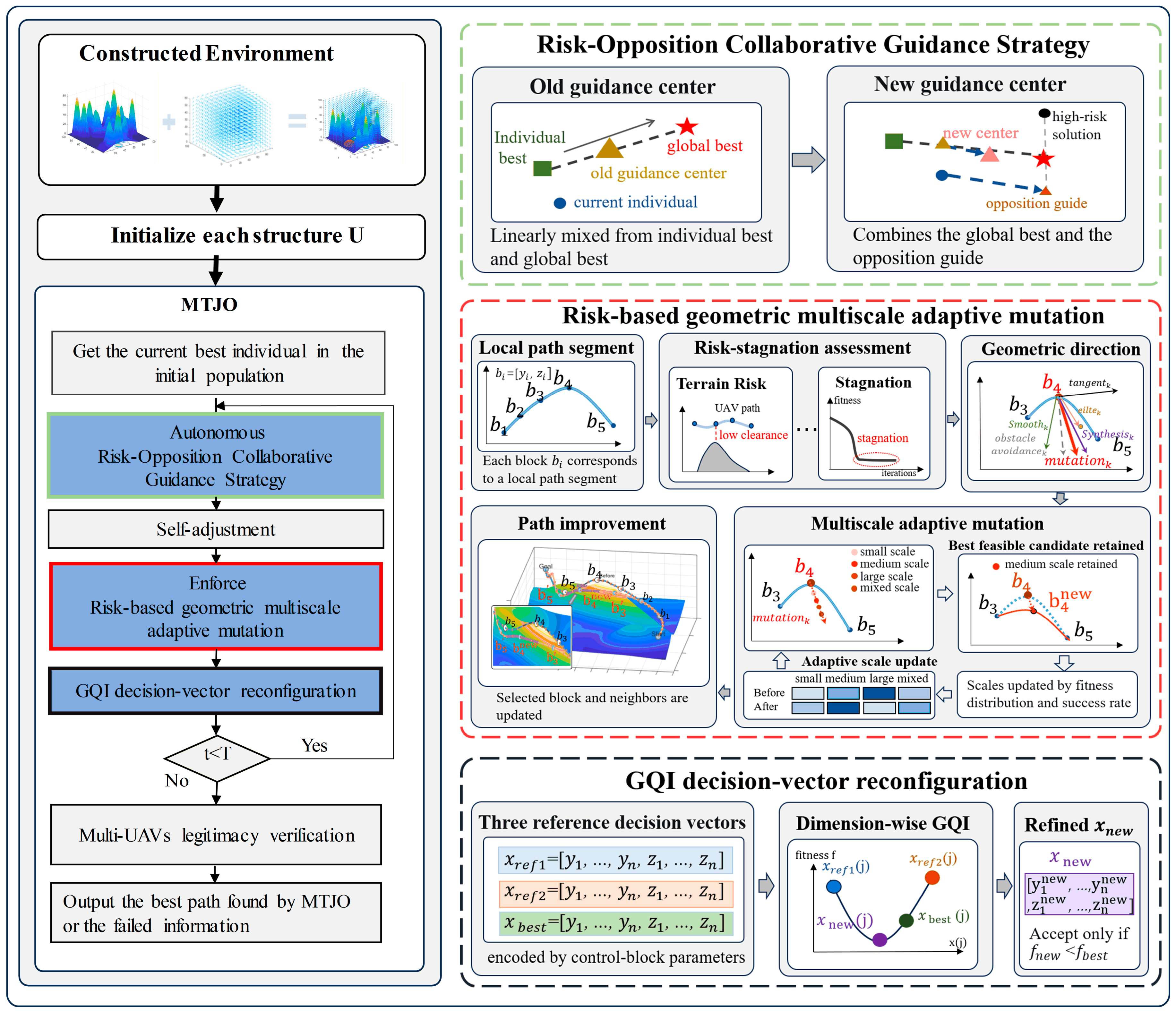
Therefore, MTJO is proposed based on the original TJO. First, a risk-opposition collaborative guidance strategy is used to correct the original guidance center, enabling the search direction to consider both global best information and risk avoidance. Second, a risk-based geometric multiscale adaptive mutation strategy is adopted to correct high-risk or stagnant local path control blocks. Finally, a GQI decision-vector reconfiguration strategy is introduced to refine the current best solution dimension by dimension during stagnation or late-stage search. These strategies enhance the algorithm from global guidance, local correction, and late-stage exploitation, respectively, as shown in Figure 2.

3.2.1. Risk-Opposition Collaborative Guidance Strategy

In the autonomous driving phase of the original TJO, individuals are mainly updated around a guidance center determined by historical best positions and the global-best position. This mechanism improves convergence by using elite solution information, but it lacks explicit feedback from path risk distributions. In offshore multi-UAV path planning, candidate trajectories are affected by island terrain, restricted fly zones, wind disturbances, and collaborative distance constraints. When some individuals are concentrated near high-risk regions, the original guidance mechanism may cause ineffective perturbations.
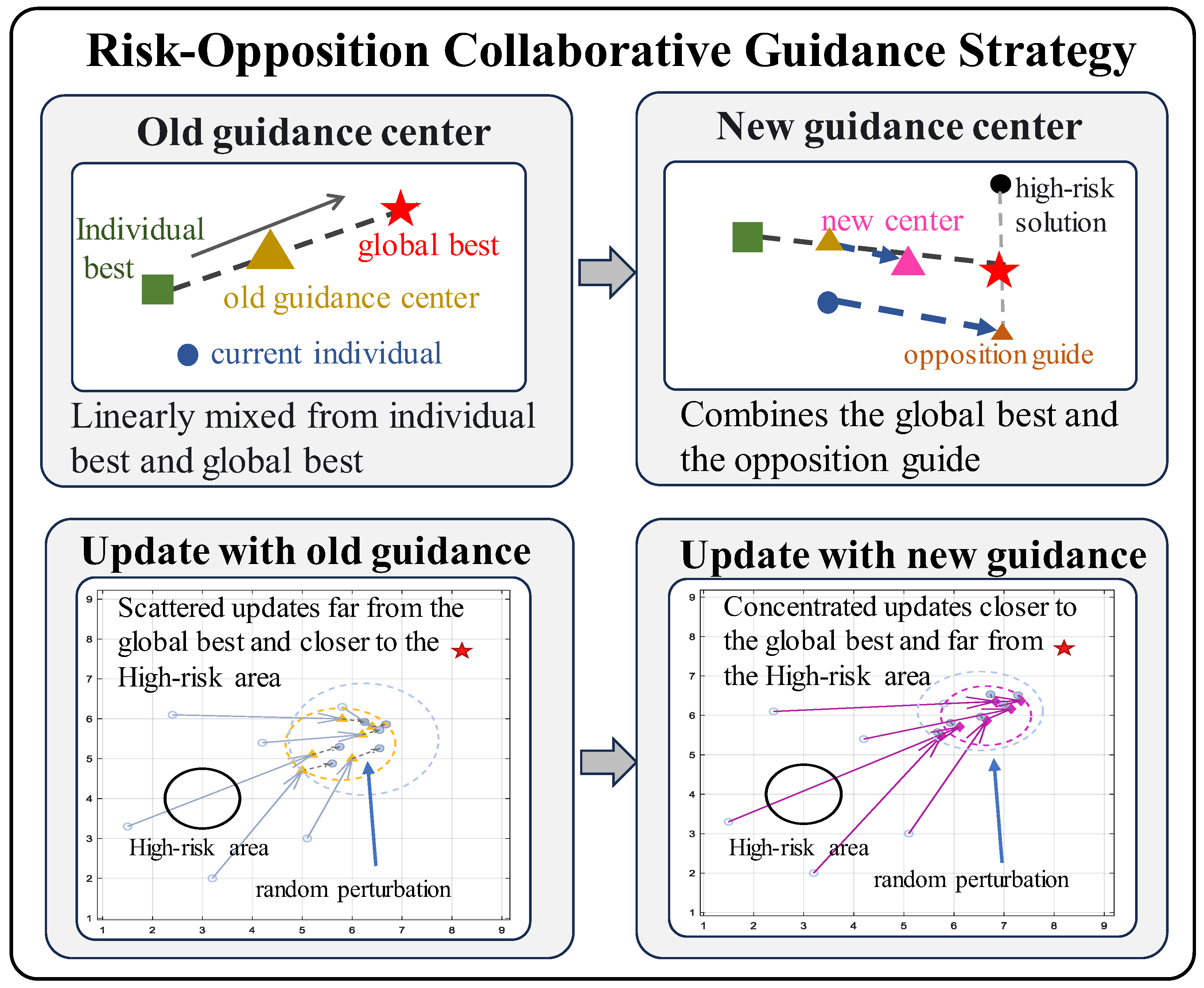
To enhance the risk awareness of the search direction, a risk-opposition collaborative guidance strategy is proposed [2,31], as shown in Figure 3. First, individuals with poor fitness values are selected to form a high-risk set H , and its center is calculated as:
x h = 1 N h x i H x i
where x h denotes the high-risk center, and N h is the number of individuals in the high-risk set. Since this paper considers a minimization problem, individuals with larger fitness values usually correspond to lower-quality trajectories or stronger constraint violations. Therefore, x h can represent the high-risk search region of the current population.
Then, taking the current best solution x b e s t as the reference, a risk-opposition direction is constructed away from the high-risk center [29]:
d o = x b e s t x h x b e s t x h
where d o denotes the unit direction from the high-risk center toward the current best solution. If the distance between x b e s t and x h is too small, the original guidance direction is retained to avoid unstable correction.
After obtaining the risk-opposition direction, an opposition guidance point is generated along this direction:
x o = x b e s t + L o d o
where x o denotes the risk-opposition guidance point, and L o is the opposition guidance step length. This step is determined by the search-space scale, iteration stage, and stagnation state so as to enhance risk avoidance in the middle-late stage or under stagnation. If x o exceeds the search boundary, it is clipped into the feasible range.
To avoid excessive disturbance to the convergence direction of the original TJO, the risk-opposition guidance point is fused with the current best solution:
x g = ( 1 μ ) x b e s t + μ x o
where x g denotes the risk-opposition guidance center, and μ is the fusion coefficient. This coefficient is adaptively adjusted with an upper bound, enabling the new guidance center to retain global-best guidance while introducing moderate risk-avoidance information.
Finally, the risk-opposition guidance center is embedded into the autonomous driving phase to correct the original basic guidance position:
B i = B 0 , i + χ D ¯ e i
where B 0 , i denotes the basic guidance position of the i-th individual in the original TJO, e i is the unit direction from the current individual to the risk-opposition guidance center, D ¯ denotes the average span of the search space, and χ is the direction correction weight. As iterations proceed, χ gradually decreases, providing stronger risk-avoidance exploration in the early stage and weaker additional perturbation in the later stage for convergence stability.
In summary, this strategy embeds risk-avoidance information into the autonomous driving phase through high-risk center identification, opposition direction construction, guidance point fusion, and directional correction. Compared with the original guidance center, the new guidance center combines the global-best position with the opposite direction of high-risk regions, guiding individuals away from high-risk areas and toward promising regions, as shown in Figure 3, thereby improving the search directionality and trajectory feasibility of MTJO in complex offshore environments.

3.2.2. Risk-Based Geometric Multiscale Adaptive Mutation Strategy

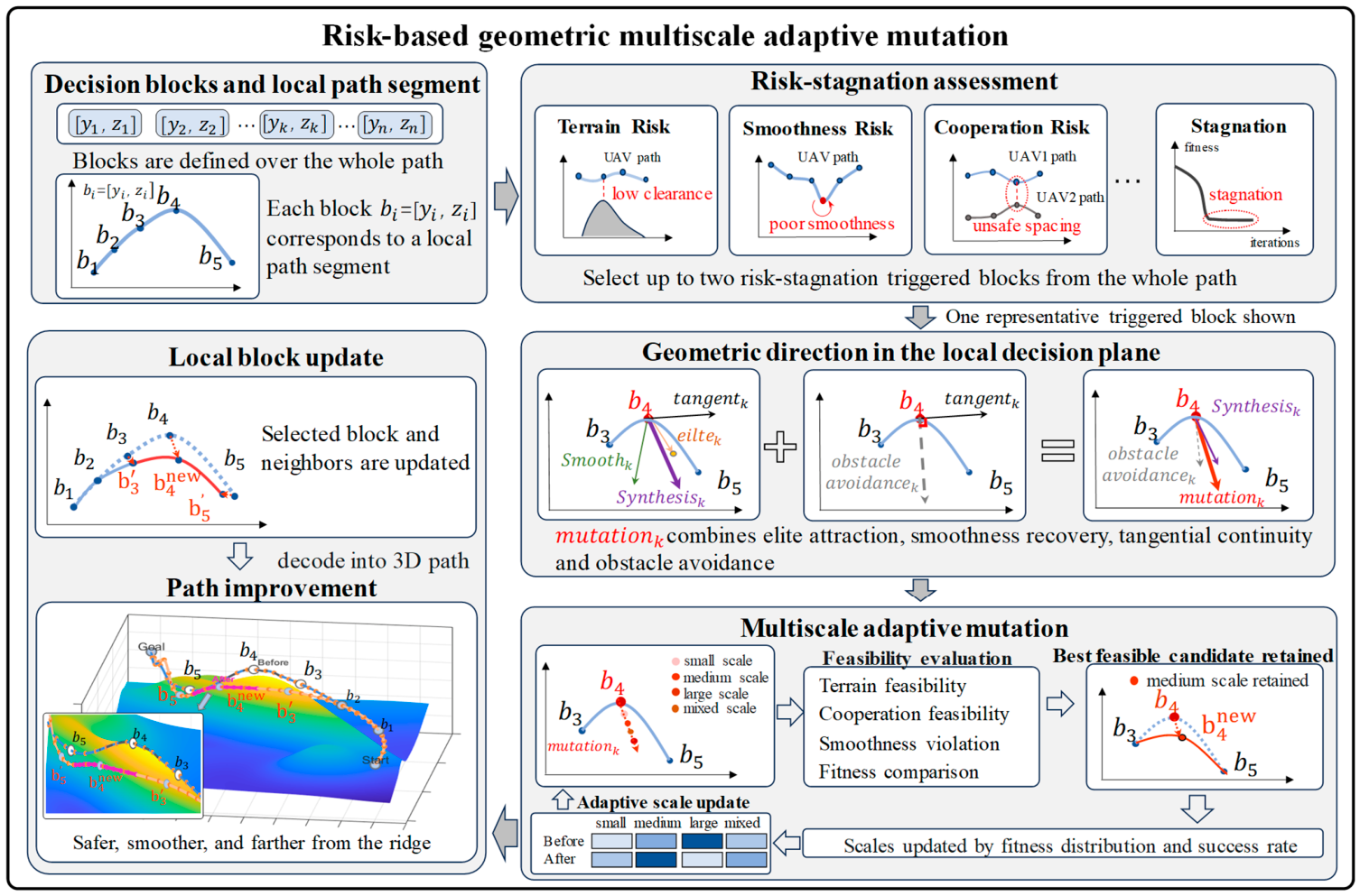
The risk-opposition collaborative guidance strategy improves population search from a global perspective, but constraint violations in offshore multi-UAV path planning often occur in local path segments. For example, low control-point altitude may cause terrain collision, large changes between adjacent control points may reduce path smoothness, and abnormal local inter-UAV distances may violate collaborative constraints. If the whole decision vector is perturbed uniformly, these local risks are difficult to correct effectively. Therefore, a risk-based geometric multiscale adaptive mutation strategy is proposed to identify high-risk or stagnant local control blocks and perform multiscale geometric correction in the local decision plane [33].
In the path-encoding scheme, each individual consists of several control points. The first half of the decision variables represents lateral offsets, while the second half represents altitudes. Thus, the lateral offset and altitude corresponding to the same control point are combined into a local decision block:
b k = [ y k , z k ] , k = 1 , 2 , , n
where b k denotes the k-th control block, and n is the number of control points. Since each block corresponds to a local path segment, block-level mutation can directly adjust local trajectory shapes.
To determine whether a control block should be mutated, both local risk and search stagnation are considered. Here, local risk does not denote a probabilistic accident risk but is defined as a deterministic surrogate indicator of the safety, feasibility, and structural quality of a local trajectory segment. For the k-th control block, the obstacle risk R k o b s describes the safety clearance between the local trajectory point and the terrain; the cooperative risk R k c o o p measures the violation of the inter-UAV safety-distance and communication-distance constraints; the smoothness risk R k s m o o t h characterizes abrupt local trajectory variations through the normalized second-order differences of adjacent control points; and the elite-deviation risk R k e l i t e represents the normalized distance between the current control block and the corresponding block of the current best solution. All four components are normalized and clipped to the interval [0, 1] to eliminate the effects of different physical units and numerical scales. The local composite risk indicator of the k-th control block is defined as follows:
R k = w o R k o b s + w c R k c o o p + w s R k s m o o t h + w e R k e l i t e
where R k denotes the local composite risk-surrogate indicator of the k-th control block; R k c o o p , R k s m o o t h and R k e l i t e denote the obstacle, cooperative, smoothness, and elite-deviation risk components, respectively; and w o ,   w c ,   w s and w o are the corresponding nonnegative weights, whose sum equals one. In this study, these weights are set to 0.35, 0.25, 0.20, and 0.20, respectively. Obstacle and cooperative risks are assigned relatively higher weights because they directly affect trajectory safety and cooperative feasibility, whereas smoothness and elite-deviation risks mainly contribute to local trajectory quality and search efficiency.
Because all four components are normalized to [0, 1]; the composite indicator R k is also bounded within [0, 1]. A larger R k indicates lower terrain clearance, more severe cooperative-distance constraint violations, greater local trajectory variation, or a larger deviation from the elite path structure. Therefore, the corresponding control block should receive a higher priority for local correction. Equation (23) is not intended to estimate the probability of an accident; instead, it provides a unified and monotonic surrogate indicator for ranking the relative risks of different control blocks and supporting mutation triggering and block selection.
The above weights were fixed a priori and remained unchanged across all two-UAV and three-UAV scenarios; they were not adjusted for any specific experimental scenario. Based on this, the mutation trigger score of each control block is defined as:
G k = β 1 Q k + β 2 R k + β 3 P
where G k is the trigger score of the k-th control block, Q k is the local stagnation score, R k is the local risk score, P is the individual stagnation flag, β 1 , β 2 and β 3 are weight coefficients. When G k exceeds a predefined threshold, the corresponding block is selected for mutation. To avoid excessive disturbance to the path structure, only a few blocks with high trigger scores are updated in each iteration.
For each selected block, a geometric mutation direction is constructed in the local decision plane. This direction combines elite attraction, smoothness recovery, and obstacle-avoidance components, which guide the block toward the current best structure, maintain continuity with neighboring control points, and move away from terrain or cooperative risk regions:
m k = a e d k e l i t e + a s d k s m o o t h + a o d k a v o i d
where m k denotes the comprehensive mutation direction of the k-th block, d k e l i t e , d k s m o o t h and d k a v o i d denote the elite attraction direction, smoothness recovery direction, and obstacle-avoidance direction, respectively, and a e , a s and a o are the corresponding weights. Compared with random perturbation, this geometric direction introduces path feasibility and local continuity information into the search process.
To handle different levels of local risk, a multiscale candidate generation mechanism is adopted. Let S denote the scale set. The candidate block generated under the q-th scale is defined as:
b k ( q ) = b k + δ q m k , q S
where δ q is the step coefficient of the q-th scale. Small-scale mutation is used for local refinement, medium-scale mutation for regular correction, large-scale mutation for escaping local stagnation, and mixed-scale mutation for improving search flexibility.
To adapt mutation scales to the search state, the scale coefficients are updated according to the current fitness distribution and the historical success rate of each scale [34]:
δ q t + 1 = clip δ q t exp ξ 1 Δ q f i t + ξ 2 Δ q s u c , δ q m i n , δ q m a x
where Δ q f i t is the scale adjustment term derived from the current fitness distribution, Δ q s u c is the adjustment term derived from the historical success rate of the q-th scale, ξ 1 and ξ 2 are control coefficients, and clip ( · ) limits the scale coefficient within a predefined range. This mechanism strengthens effective scales and weakens ineffective ones.
Since mutating a single control block may break the continuity of adjacent path segments, the triggered block and its neighboring blocks are updated collaboratively with attenuation:
b k + r n e w = b k + r + ζ r δ q m k , r { 1 , 0 , 1 }
where ζ r is the neighborhood attenuation coefficient. r = 0 denotes the triggered core block, while r = 1 and r = 1 denote its neighboring blocks. This update reduces sharp turns caused by single-point mutation and improves local trajectory smoothness.
After candidate solutions are generated, a feasibility-first and fitness-second selection rule is adopted. Let C be the candidate set, V ( x ) denote the constraint violation degree, and F ( x ) denote the overall fitness. The candidate selection process is expressed as:
x n e w = arg min x C V ( x ) , F ( x )
This rule first retains candidates with smaller constraint violations. When feasibility is identical or similar, the overall fitness is compared. Thus, paths with severe terrain collision or cooperative distance violations are avoided even if they provide lower fitness values.
In summary, this strategy uses path control blocks as basic units and integrates local risk identification, stagnation detection, geometric directional correction, and multiscale adaptive search, as shown in Figure 4. It can correct high-risk local path segments directionally, improve path feasibility, and preserve trajectory smoothness, thereby enhancing the local refinement ability of the original TJO.

3.2.3. GQI Decision-Vector Reconfiguration Strategy

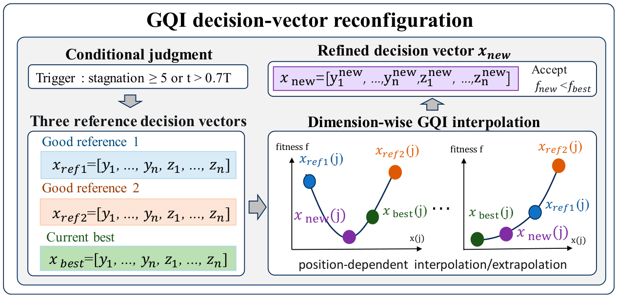
After risk-opposition guidance and multiscale local mutation, MTJO obtains strong global risk-avoidance ability and local trajectory correction ability. However, in the later search stage or when the current best solution remains unchanged for several iterations, the population may still concentrate in a local region, making further improvement difficult. To enhance late-stage exploitation, a GQI decision-vector reconfiguration strategy is introduced to refine the current best individual through dimension-wise interpolation or extrapolation [30], as shown in Figure 5.
In MTJO, the GQI refinement operation is triggered when the current best solution stagnates for a predefined number of iterations or when the algorithm enters the late search stage. Let the current best individual be x b e s t , with fitness f b e s t . Two high-quality reference individuals different from x b e s t are selected from the current population and denoted as x r e f 1 and x r e f 2 , with fitness values f r e f 1 and f r e f 2 , respectively. These three decision vectors form the reference set for GQI reconfiguration:
R = x r e f 1 , f r e f 1 , x r e f 2 , f r e f 2 , x b e s t , f b e s t
For the j-th decision variable, the three reference points are reordered according to fitness and denoted as x r e f 1 , f r e f 1 ,   x r e f 2 , f r e f 2 ,   x b e s t , f b e s t . GQI estimates a potentially better position in this dimension using three-point quadratic interpolation [30]:
x n e w ( j ) = ( x j 2 x k 2 ) f i + ( x k 2 x i 2 ) f j + ( x i 2 x j 2 ) f k 2 ( x j x k ) f i + ( x k x i ) f j + ( x i x j ) f k + ε
where x n e w ( j ) denotes the j-th variable of the reconfigured decision vector and is a small constant used to avoid division by zero. Equation (31) gives the basic quadratic interpolation kernel used in GQI. Unlike ordinary quadratic interpolation, GQI adaptively selects direct interpolation or constructs extrapolated reference points according to the relative positions of the three reference points in the current dimension, thereby improving adaptability under different local distributions. If the interpolation result is invalid or exceeds the boundary, the variable is remapped into the feasible range, followed by boundary repair after the complete vector is generated.
After GQI reconstruction is completed for all dimensions, a new candidate decision vector is obtained:
x n e w = [ x n e w ( 1 ) , x n e w ( 2 ) , , x n e w ( d ) ]
Then, x b e s t is decoded into a three-dimensional path, and its overall fitness f n e w is recalculated. To prevent ineffective refinement from damaging the current best solution, a strict acceptance rule is adopted:
x b e s t = x n e w , f n e w < f b e s t , x b e s t , f n e w f b e s t .
Thus, the GQI decision-vector reconfiguration strategy updates the current best individual only when a better solution is generated, ensuring that the existing best path quality is not degraded. This strategy exploits high-quality information in the current population during stagnation or late-stage search, thereby improving the local exploitation ability and final path quality of MTJO.

3.3. The Framework of MTJO

Based on the three-phase search structure of the original TJO, the proposed MTJO introduces three improvement strategies: risk-opposition collaborative guidance, risk-based geometric multiscale adaptive mutation, and GQI decision-vector reconfiguration. The overall framework is shown in Figure 2. MTJO retains the main update mechanism of TJO, while embedding risk-aware guidance, local control-block correction, and late-stage refinement into the iterative process.
At the beginning, the population of each UAV is initialized using Equation (4) and Equation (5). Each individual is decoded into a three-dimensional path, and its fitness is calculated using Equation (6). Then, the personal memory, global best solution, and current best path of each UAV are initialized.
In each iteration, MTJO first constructs the risk-opposition guidance center using Equations (17)–(20), and corrects the original TJO guidance position using Equation (21) Based on the corrected guidance position, the autonomous driving, self-regulation, and enforcement phases are performed according to Equation (9), Equation (11), and Equation (13), respectively, followed by boundary handling using Equation (15). The updated individuals are then decoded into paths, and their temporary fitness values are calculated.
After the main TJO update, MTJO evaluates the risk and stagnation states of local path control blocks using Equations (22)–(24). For the triggered blocks, geometric multiscale mutation candidates are generated using Equations (25)–(28), and the best feasible candidate is selected according to Equation (29). After mutation, boundary handling is performed again, and the mutated individuals are decoded and re-evaluated. Then, the personal memory, global best solution, and current best path are updated according to the new fitness values.
When the current best solution stagnates or the iteration enters the late search stage, GQI decision-vector reconfiguration is triggered. Reference vectors are selected using Equation (30), and the current best individual is refined dimension by dimension using Equations (31) and (32). The refined solution is accepted only if it satisfies Equation (33). Finally, MTJO outputs the best path of each UAV and the corresponding convergence curve.
The complete optimization procedure of MTJO is summarized in Algorithm 1.
Algorithm 1: The Pseudocode for MTJO
  • for each UAV do
  •  Initialize population positions using Equations (4) and (5).
  •  Decode each individual into a 3D path.
  •  Calculate fitness values using Equation (6).
  •  Initialize personal memory, global best solution, and BestPath of UAV.
  •  Set stagnation counter and mutation state.
  • end for
  • for t = 1 to T do
  •  for each UAV do
  •   Obtain current population, personal memory, and global best solution.
  •   Construct the risk-opposition guidance center using Equations (17)–(20).
  •   Generate the original TJO guidance position and correct it using Equation (21)
  •   Perform autonomous driving update using Equation (9).
  •   Perform self-regulation update using Equation (11).
  •   Perform enforcement update using Equation (13).
  •   Apply boundary handling using Equation (15).
  •   Decode updated individuals into 3D paths.
  •   Calculate temporary fitness values using the comprehensive cost function.
  •   Evaluate local control blocks using Equations (22)–(24).
  •   Generate geometric multiscale mutation candidates using Equations (25)–(28).
  •   Select the best feasible candidate using Equation (29).
  •   Apply boundary handling again.
  •   Decode the mutated individuals into 3D paths.
  •   Recalculate fitness values.
  •   Update personal memory according to fitness comparison.
  •   Update the global best solution and BestPath of UAV.
  •   Update the stagnation counter.
  •   if stagnation condition is satisfied or t enters the late search stage then.
  •    Select reference vectors using Equation (30).
  •    Perform GQI decision-vector reconfiguration using Equations (31) and (32).
  •    Accept the refined solution according to Equation (33).
  •    Update BestPath of UAV if refinement succeeds.
  •   end if
  •   Record the best fitness of UAV.
  •  end for
  •  Record cost components of the current best paths.
  • end for
  • return the best path of each UAV and convergence curve.

3.4. Time Complexity Analysis

Let N denote the population size, T the maximum number of iterations, d the decision-variable dimension, n the number of path control points, and S the multiscale set. In the initialization stage, MTJO generates N individuals with d dimensions and evaluates their initial fitness values, resulting in a time complexity of O N d .
In each iteration, the autonomous driving, self-regulation, enforcement, boundary handling, and fitness update operations of the original TJO are performed on data with size N × d , so the main update complexity is O N d . The risk-opposition collaborative guidance strategy selects high-risk individuals and calculates the risk-aware guidance center. If sorting is used to obtain the high-risk set, its complexity is O ( N log N + N d ) , with limited additional cost.
The risk-based geometric multiscale adaptive mutation strategy evaluates the risk state of path control blocks and generates multiscale candidates for a small number of triggered blocks. Since n = d / 2 , and both the number of triggered blocks and | S | are small constants, this part can still be regarded as O N d . The GQI decision-vector reconfiguration strategy is triggered only during stagnation or the late search stage and acts only on the current best individual. Its single-trigger complexity is O d plus one fitness evaluation, which does not change the overall complexity order.
Therefore, the main computational cost of MTJO comes from population position updating and fitness evaluation. When the number of triggered blocks, the size of the multiscale set, and the number of GQI triggers are regarded as bounded constants, the overall time complexity of MTJO is O N d T .
This result suggests that the proposed strategies enhance the original TJO without introducing substantial computational overhead. They enhance risk-aware search and local refinement without changing the overall time complexity order.

4. MTJO-Based Cooperative Path Planning for Marine Multi-UAV Missions

This section applies MTJO to the marine multi-UAV cooperative path planning problem. It first defines the UAV performance constraints and the collaborative constraints among UAVs. Then, the comprehensive cost function and the encoding relationship between three-dimensional trajectories and algorithm individuals are described. Finally, the MTJO-based procedure for generating cooperative UAV trajectories is presented.

4.1. UAV Performance Constraints

Actual UAV flight is limited by propulsion systems, maneuverability, and communication performance. Therefore, the planned trajectories should satisfy basic performance constraints. This study mainly accounts for flight speed, maximum yaw angle, communication-range limitation, and minimum separation requirement, which provide the basis for path feasibility checking and cost function design [15,35].

4.1.1. Speed Range Limitation

The allowable speed range specifies the feasible velocity interval for a UAV during mission execution [35]. Due to limitations of the propulsion system and aerodynamic characteristics, the UAV speed should satisfy both minimum and maximum speed requirements to ensure flight stability and mission feasibility. In this paper, the speed range is set according to different experimental scenarios, with the specific values provided in the experimental setup.

4.1.2. Yaw-Angle Limitation

Limited by aerodynamic characteristics, propulsion systems, and flight control capability, UAVs cannot perform excessive direction changes. If the deflection angle or climb angle between adjacent path segments exceeds the allowable range, the planned path may be difficult to track in practice. Accordingly, constraints are imposed on horizontal heading changes and vertical ascent/descent inclination, and both angular limits are specified as 45° [7].

4.1.3. Communication Range and Safety Separation Limits

In multi-UAV cooperative missions, the distance between UAVs directly affects communication connectivity and flight safety. Excessive distance may cause communication interruption, while overly short distance may increase collision risk. To support feasible cooperation among UAVs, the model incorporates an upper limit on communication range and a lower limit on inter-UAV separation. In the experiments, these two thresholds are specified as 40 km for communication connectivity and 3 km for collision avoidance, respectively [7,8].

4.2. Multi-UAVs Collaborative Constraint

Unlike single-UAV path planning, multi-UAV path planning should also consider inter-UAV cooperation. In this paper, collaborative constraints are established from two aspects: distance cooperation and time cooperation. The former ensures communication connectivity and flight safety, while the latter coordinates UAVs to arrive at the target area as synchronously as possible under speed constraints.

4.2.1. Distance Constraints

Due to communication and safety requirements, UAVs should maintain appropriate distances during cooperative flights. Excessive distance may cause communication interruption, while overly short distance may increase collision risk. Accordingly, each pair of UAVs must maintain an inter-UAV distance that is no smaller than the safety threshold and no larger than the communication threshold. The distance between corresponding trajectory points is calculated as:
d j , k = ( x j ( e ) x k ( f ) ) 2 + ( y j ( e ) y k ( f ) ) 2 + ( z j ( e ) z k ( f ) ) 2
where d j , k denotes the distance between the trajectories of the j-th and k-th UAVs, x j e ,   y j e ,   z j e and x k f ,   y k f ,   z k f denote the corresponding path points of the j-th and k-th UAVs, respectively, and j k . After introducing the time constraint, e = f can be used to compare path points under the same time sequence.

4.2.2. Time Constraints

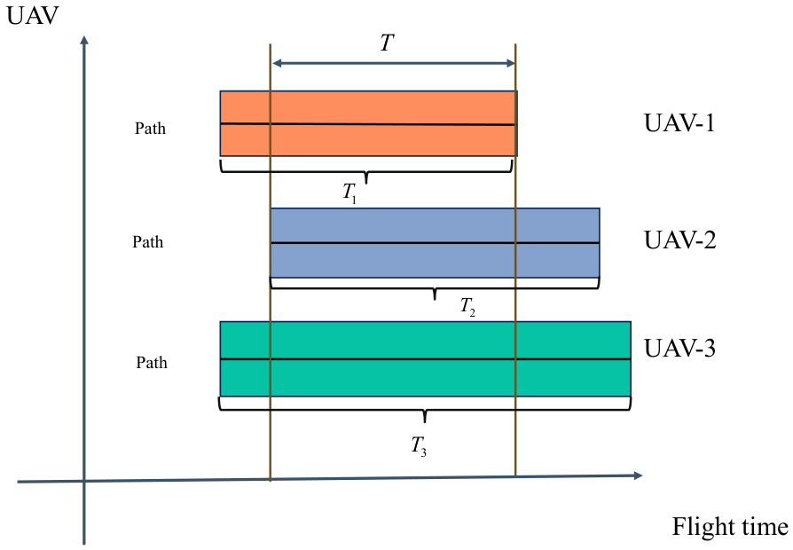
In offshore emergency cooperative missions, simultaneous arrival of multiple UAVs at the target area can improve response efficiency and cooperative coverage. Therefore, the feasible flight time interval of each UAV is calculated according to its speed range and path length, and the intersection of these intervals is used to determine whether synchronous arrival is feasible [7,8].
For the i-th UAV, let D i be its path length, and v i , max and v i , min be its maximum and minimum speeds, respectively. The feasible flight time interval is:
T i D i v i , m a x , D i v i , m i n
Once the feasible time ranges of all UAVs are calculated, their overlap is used to identify the shared arrival-time interval:
T = T 1 T 2 T p
If T is non-empty, the current path combination satisfies the time coordination requirement. When a common interval exists, the velocity of each UAV can be adjusted within this interval to enable simultaneous arrival at the target area. For time-critical offshore emergency operations, the earliest feasible coordinated arrival is obtained from the lower endpoint of T. The time-feasibility judgment procedure is illustrated Figure 6 [7].
This constraint enforces synchronized arrival among UAVs; therefore, the reported flight times of different UAVs under the same algorithm may be identical or very close when the constraint is satisfied.

4.3. Cost Function

In complex offshore environments, multi-UAV path planning should consider path length, smoothness, environmental risks, and collaborative constraints. Therefore, a comprehensive cost function is constructed to evaluate candidate trajectories, as shown in Equation (37):
C = w 1 C l + w 2 ( C l C r ) + w 3 C s + w 4 C v + w 5 C t + w 6 C d
In Equation (37), the weight coefficients w 1 ,   w 2 ,   w 3 ,   w 4 ,   w 5 and w 6 adjust the contribution of each sub-cost term. C l denotes the path length cost, C s denotes the path smoothness cost, C r denotes the restricted flying area cost, C v denotes the wind field cost, C t denotes the terrain threat cost, and C d denotes the multi-UAV distance constraint cost. The sub-cost functions are defined as follows [7].

4.3.1. Path Length

The path-length term reflects the spatial efficiency of a trajectory. Reducing this term can lower energy demand and shorten the arrival time. It is computed as the cumulative Euclidean distance of adjacent path points, as given in Equation (38):
C l = j = 1 n 1 R j R j + 1
In Equation (38), R j R j + 1 is the adjacent-point distance vector, R j R j + 1 denotes its Euclidean norm, where n denotes the total count of trajectory points.

4.3.2. Trajectory Smoothness Cost

Path smoothness evaluates trajectory continuity and trackability. Due to UAV maneuverability limits, excessive deflection and climb angles should be avoided. The trajectory smoothness cost is defined in Equation (39) [15,35]:
C s = j = 1 n 1 θ j + j = 1 n 1 φ j
where n is the number of sampled points along the trajectory, θ j and φ j correspond to the horizontal turning component and vertical climbing component at the j-th path point, respectively.
(1)
Horizontal Deflection Components
Heading variation in the Oxy plane is used to quantify horizontal turning behavior, and its value is computed according to Equation (40):
θ j = a r c t a n R j R j + 1 × R j + 1 R j + 2 R j R j + 1 · R j + 1 R j + 2 θ j = | θ j | , i f   | θ j | > θ m a x 0 , o t h e r w i s e
In Equation (40), R j R j + 1 represents the forward-vector projection on the Oxy plane, while θ m a x is the prescribed upper limit of the deflection angle.
(2)
Climbing-Angle Components
The climb angle measures the vertical inclination between a path segment and the horizontal plane, and it is computed by Equation (41):
φ j = a r c t a n z j + 1 z j R j R j + 1 φ j = φ j φ j 1 , i f   φ j φ j 1 > φ m a x 0 , o t h e r w i s e
In Equation (41), R j R j + 1 corresponds to the vector between adjacent trajectory points, z j gives the z-axis coordinate at the j-th point and φ m a x defines the maximum permitted climbing inclination.

4.3.3. Wind Disturbance Cost

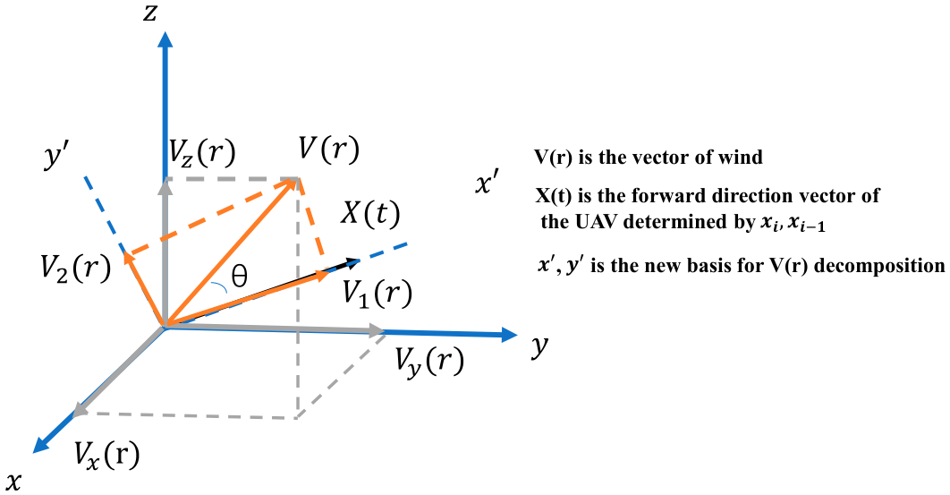
The wind disturbance cost is used to quantify the influence of marine wind on UAV trajectory execution. The known wind vector is projected onto the tangential and normal directions of the trajectory to evaluate the assisting/resisting effect and lateral yaw disturbance, respectively [7,13]. First, the wind intensity at each path point is calculated using Equation (42) and then decomposed into tangential and normal components using Equation (43). Since the decomposed value may be negative, Equation (44) is used to map it into a unified interval:
V k r = V x ( r ) 2 + V y ( r ) 2 + V z ( r ) 2
C ˜ v = k = 1 p ( V k ( r ) · cos θ V k ( r ) · sin θ )
C v = a a 1 + e C ˜ v b
In Equation (42), V k ( r ) denotes the wind intensity at path point k, θ is defined as the direction gap between UAV motion and the sea-wind vector, and p indicates how many discrete points are used along the trajectory. V k ( r ) c o s ( θ ) and V k ( r ) sin ( θ ) correspond to the tangential and normal wind-effect terms, respectively. The tangential term reflects whether the wind assists or opposes UAV motion, while the normal component is used to capture crosswind-induced lateral deviation. The corresponding sea wind cost calculation is shown in Figure 7 [7].

4.3.4. Restricted Flying Area

The restricted flying area cost penalizes trajectories entering high-risk regions. This cost term is formulated using the separation between trajectory points and restricted-area centers, together with the assigned risk levels, as expressed in Equation (45) [16,17]
C r = j = 1 T r l j m e a n ( i = 1 n ( ε ( 1 d i , 0.0 j R j ) + ε ( 1 d i , 0.1 j R j ) + + ε ( 1 d i , 0.9 j R j ) ) )
In Equation (45), n is the trajectory-point count, T r represents the number of flight-restricted regions, l j is the risk coefficient associated with region j, and ε denotes a step activation function. This activation function prevents the restricted-region penalty from being included when the UAV is outside the corresponding region. For numerical implementation, 10 intermediate samples are added between every two neighboring trajectory points. The distance term for the j-th restricted region is then evaluated using the mean separation over all sampled points.

4.3.5. Terrain Area

The terrain cost determines whether the trajectory collides with island terrain. If the flight altitude is lower than the terrain height at the corresponding position, the path is regarded as infeasible and this cost is set to infinity [14]:
C t = 0 , i f   z k H t e r r a i n ( x k , y k ) > 0 , o t h e r w i s e
In this formula, H t e r r a i n ( x k , y k ) is the terrain elevation sampled at point k, while z k denotes the UAV flight height at the same spatial location.

4.3.6. Multi-UAVs Distance Constraints

To evaluate violations of safety separation and communication-range requirements among UAVs, an inter-UAV distance penalty is defined as follows [7,8]:
C d = i = 1 n u m 1 k = 1 n d i , k , i f   d i , k > d l o n g i = 1 n u m 1 k = 1 n 10000 / d i , k , e l s e i f   d i , k < d s h o r t 0 , o t h e r w i s e
In Equation (47), d s h o r t and d l o n g are the lower safety threshold and upper communication threshold for inter-UAV distance, respectively. d i , k is used to measure the distance from the UAV under evaluation to trajectory point k of U A V i , and num denotes the number of UAVs involved in the mission.

4.4. Path-Planning Method

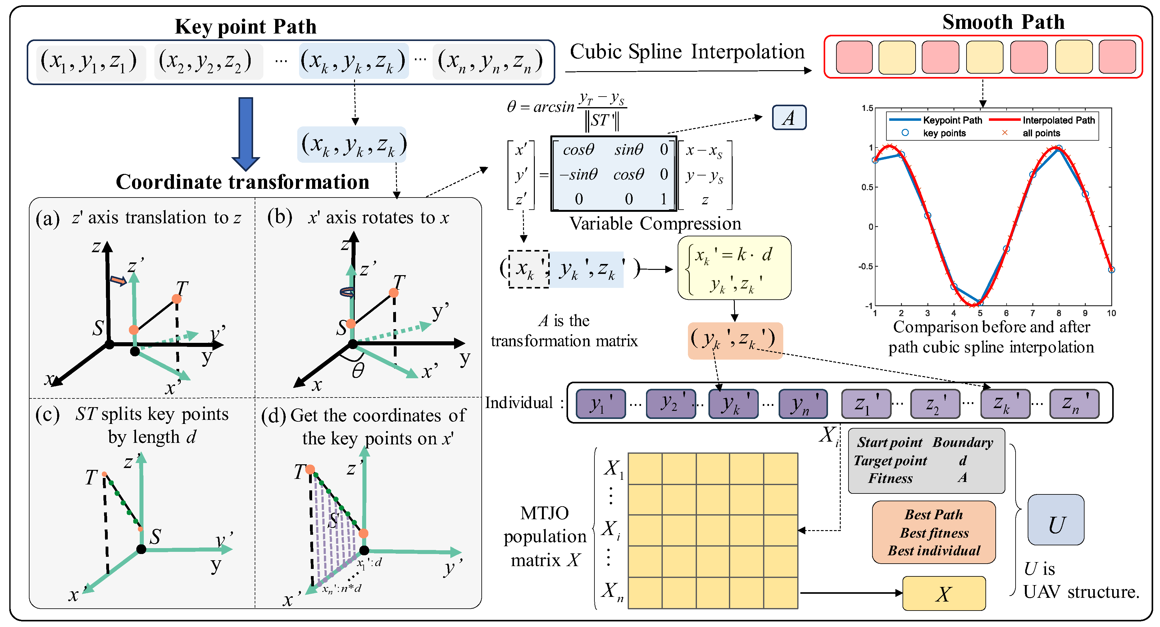
Figure 8 [7] shows how the MTJO search variables are mapped to UAV trajectory generation. A single-UAV route is encoded by several spatial control points, whose coordinates are optimized by MTJO during iteration. After the key points are obtained, cubic spline interpolation is adopted to construct a smooth trajectory-point sequence, which forms the continuous flight route.
To reduce the dimension of individuals, coordinate transformation is adopted to reduce the search space. In the transformed coordinate system, the x′-coordinates of key points are determined by the start point, target point, and the number of key points. Let ST denote the line segment connecting the start point S and the target point T. By evenly dividing the projection of ST on the x′-axis, the spacing d between key points can be obtained, and the x′-coordinates are determined accordingly. As a result, MTJO performs optimization only on the y′- and z′-coordinate components of the key points.
For each individual, the y′- and z′-coordinate components of all key points are encoded as its decision vector, and multiple individuals constitute the population of the corresponding UAV. During iteration, each individual represents a candidate trajectory. To facilitate computation and information storage, a dedicated data structure U is created for every UAV to manage the variables involved in trajectory encoding, evaluation, and optimization.

4.4.1. Path Solution Framework

From an optimization perspective, path planning aims to search for an optimal solution among multiple feasible trajectory candidates. For multi-UAV path planning, each candidate trajectory satisfying the basic constraints corresponds to a feasible solution, and the objective is to search for the path combination with the minimum comprehensive cost.
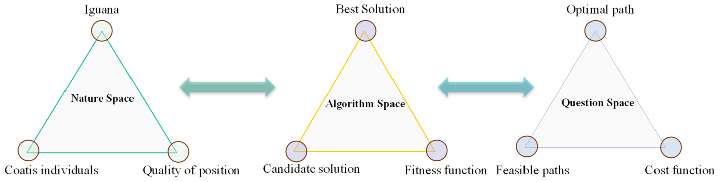
The MTJO iteration process is driven by three key components: population individuals, elite solutions, and objective-function evaluation. In the context of trajectory optimization, candidate solutions correspond to UAV candidate trajectories, the best individual in the population corresponds to the current best path, and the comprehensive path cost function serves as the fitness function to evaluate trajectory quality. By continuously updating population individuals, MTJO gradually guides the search process toward better paths. The correspondence among the natural inspiration mechanism, algorithm elements, and path planning components is shown in Figure 9.

4.4.2. Coordinate Transformation

To simplify the optimization dimension of the path-planning problem, this paper adopts a coordinate transformation method to simplify the path search space. For each UAV, the known start point S and target point T are used to construct a reference segment ST. In the transformed coordinate frame, S is aligned with the z′-axis, while ST is constrained to lie on the Oxz′-plane, so that the x′-coordinates of the path key points can be predetermined by the start point, target point, and number of key points. Therefore, the algorithm only needs to optimize the y′- and z′-coordinates [7].
The coordinate transformation consists of two steps: translation and rotation. First, the original coordinate system is translated so that the start point S is aligned with the z′-axis in the target coordinate system. Then, the coordinate system is rotated around the z-axis by an angle θ , thereby placing segment ST on the Oxz′-plane. The rotation angle θ is determined from the projection of ST on the Oxy-plane relative to the x-axis. Let the coordinates of the key point in the target coordinate system be (x′, y′, z′) and the coordinates in the original coordinate system be (x, y, z). The relationship between them is shown in Equation (48):
θ = a r c s i n y T y S S T x y z = c o s θ s i n θ 0 s i n θ c o s θ 0 0 0 1 x x S y y S z
In Equation (48), θ denotes the rotation angle around the z-axis, y S and y T are the coordinate values associated with the departure and destination points, respectively, and ST′ denotes the vector obtained by projecting segment ST onto the Oxy-plane. This coordinate transformation can reduce the number of optimization variables and provide a concise path encoding method for MTJO to search feasible 3D trajectories.

4.4.3. Multi-UAV Information Storage

For unified management of the multi-UAV path planning process, each UAV is assigned a data structure U, which records the start point, target point, population information, variable bounds, fitness values, the key-point spacing d in the x′-axis direction, and the coordinate transformation matrix. In the cost-calculation stage, the optimized key points are transformed back to the original coordinate frame through inverse mapping, thereby recovering the actual three-dimensional trajectory. The best path in the population is stored as the current optimal trajectory of the UAV.

4.4.4. Trajectory Smoothing via Cubic Splines

Since only a small set of key points is generated during MTJO optimization, directly connecting them may lead to insufficient smoothness. Therefore, cubic spline interpolation is used to generate continuous path points, and the path cost is calculated based on the interpolated trajectory [7]. The interpolated path segment is expressed as:
L j = A j u 3 + B j u 2 + C j u + D j
In this expression, j = 1, 2, …, n, with u constrained to [0, 1]. Here, n gives the number of sampled trajectory points, whereas A, B, C, and D correspond to the cubic-spline coefficients within the considered interval.

4.5. Improved MTJO Procedure for Coordinated Multi-UAV Trajectories

To apply the improved MTJO to offshore multi-UAV cooperative path planning, path encoding, collaborative constraint evaluation, and swarm optimization are organized in a unified framework. Each UAV corresponds to an independent population, and each individual in the population represents a candidate trajectory of that UAV. During iteration, the algorithm evaluates candidate paths using the comprehensive cost function and calculates collaborative constraint costs based on the current best trajectories of other UAVs, thereby considering both single-UAV path performance and multi-UAV cooperation.

4.5.1. Guidance-Based Cooperative Evaluation

During multi-UAV path planning, candidate trajectories of different UAVs are continuously updated. Since safety distance and communication distance constraints exist among UAVs, the evaluation of one UAV trajectory depends not only on its own path quality, but also on the current trajectory states of other UAVs. Therefore, a collaborative evaluation mechanism based on current best trajectories is adopted.
In each iteration, the current best path of each UAV population is used to represent its temporary trajectory state. When evaluating a candidate path of the i-th UAV, the algorithm reads the current best paths of other UAVs and calculates the distances between corresponding path points. When the inter-UAV distance violates either the safety threshold or the communication threshold, the corresponding penalty is included in the comprehensive cost function. Once all UAV populations have been updated in the current iteration, the search enters the next iteration. This mechanism allows inter-UAV collaborative constraints to be embedded throughout the MTJO optimization process.

4.5.2. Overall Procedure for Coordinated UAV Trajectory Generation

Figure 2 summarizes the main steps involved in the proposed multi-UAV cooperative path planning method, whose main steps are summarized below.
First, a three-dimensional offshore environment model is constructed. According to the simulation parameters, the positions, numbers, and risk levels of restricted flying areas are determined. The Lamb-Oseen function is adopted to represent the marine wind field, and the island terrain is produced based on a mixed Gaussian function.
Second, a local trajectory coordinate frame is built for each UAV using its departure and destination points. The corresponding transformation matrix and fixed key-point spacing d are then calculated, and the UAV trajectory data structure U is initialized. During initialization, each UAV population randomly generates initial individuals within the corresponding search boundaries, and initial candidate trajectories are obtained through path decoding.
Then, the improved MTJO is used to iteratively update each UAV population. Each individual is transformed back to the original coordinate system and smoothed by cubic spline interpolation to generate a three-dimensional trajectory, whose fitness is calculated using the comprehensive cost function. During fitness evaluation, the current best trajectories of other UAVs are used as collaborative references to calculate inter-UAV distance constraint costs, guiding the algorithm to search for path combinations satisfying multi-UAV cooperation requirements.
Finally, after the iteration limit is met, the best solution from each UAV population is decoded into its corresponding trajectory. The resulting multi-UAV path set is further checked using the distance-related and timing-related coordination requirements. If these requirements are met, the path set is output as the final cooperative solution; otherwise, it is identified as infeasible and a failure message is returned.

5. Experimental Evaluation and Analysis

To examine the optimization capability of the proposed MTJO, two offshore simulation scenarios are designed, and cooperative path planning experiments are conducted for two UAVs and three UAVs, respectively. The experimental environment includes marine wind fields, island terrain, and restricted fly zones, which are used to simulate multiple constraints in complex offshore mission spaces. Path planning results in different scenarios are used to evaluate the path search ability, constraint handling ability, and multi-UAV cooperative performance of MTJO.
In the experiments, the parameters r d ¯ and ζ of the Lamb-Oseen model are set to 3 and 5, respectively. The population contains 100 individuals, and each path is represented by 10 key points. Accordingly, the dimension of each individual is 20, and the iteration limit is set to 100. The cost–function parameters are set as follows: w 1 = 2, w 2 = 20, w 3 = 2, w 4 = 300, w 5 = 1, and w 6 = 1. After cubic spline interpolation, each trajectory contains 50 path points. HHO WOA, ISSA, TJO, and FTO are selected as comparison algorithms. In each scenario, every algorithm is run independently 10 times. For each run, the comprehensive cost of the best path is recorded, including the minimum, maximum, average, and variance, are calculated from the 10 independent runs. For the multi-UAV system, the collaborative cost is evaluated by averaging the mean costs obtained for all UAVs.
The experiments were carried out in MATLAB R2024b (24.2.0.2712019) on a 64-bit Windows PC with an Intel(R) Core (TM) i7-14650HX CPU at 2.20 GHz, 16.0 GB of RAM, and an NVIDIA GeForce RTX 4050 Laptop GPU with 6 GB of memory.

5.1. Experimental Setup

To evaluate the optimization performance of the proposed MTJO, five algorithms are selected for comparison, including Harris Hawks Optimization (HHO) [36], the classical swarm intelligence algorithm WOA [26], the Improved Salp Swarm Algorithm ISSA [37,38], the original TJO [29], and the recently proposed physics-inspired FTO [39]. All algorithms use the same path encoding method, environment model, constraints, and comprehensive cost function to ensure fair comparison. The main parameter settings of each algorithm are summarized in Table 1. Table 2 and Table 3 present the initial and terminal positions, speed ranges, and inter-UAV distance settings used in the two-UAV and three-UAV experiments, respectively. The environmental parameters are listed in Table 4.
In MTJO, w d i r = 0.18(1 − t/T) is used as a decreasing directional-guidance weight, where t and T denote the current and maximum iteration numbers, respectively. A relatively larger value in the early stage helps strengthen risk-opposition guidance, while the decreasing form reduces excessive perturbation in the later stage. The high-risk ratio of 0.25 determines the proportion of poorly performing or high-risk individuals used for high-risk region identification. The fusion upper bound of 0.10 limits the maximum influence of the guidance term on the position update, thereby preventing excessive directional deviation. The scale coefficients {0.02, 0.06, 0.14} define the small, medium, and large mutation amplitudes used in the geometric multiscale adaptive mutation strategy.

5.2. Experimental Analysis

5.2.1. Two UAVs Case

(1)
Scenarios 1
Scenario 1 contains four flight-restricted regions assigned with different risk coefficients. In this scenario, the Lamb-Oseen model is adopted to describe the marine wind field, while a mixed Gaussian surface is used to represent the island terrain.
Table 5 reports the statistical results of 10 independent runs, while Table 6 presents the corresponding path lengths and synchronized flight time.
As shown in Table 5, MTJO achieves the lowest mean cost for both UAVs. For UAV-1, the mean cost of MTJO is 202.2907, which is reduced by 55.23%, 6.96%, 14.32%, 36.09%, and 23.00% compared with HHO, FTO, WOA, ISSA, and TJO, respectively. For UAV-2, MTJO obtains a mean cost of 189.7514, reducing the cost by 71.93%, 12.59%, 35.42%, 44.55%, and 28.57%, respectively. In addition, the standard deviations of MTJO are 9.9122 and 10.6126, which are much lower than those of HHO, WOA, ISSA, and TJO, indicating good stability over repeated runs.
Table 6 shows that MTJO generates compact paths. The path length of UAV-1 is 97.2696 km, which is the shortest among all algorithms. For UAV-2, the path length obtained by MTJO is 87.1438 km, which is slightly longer than that of ISSA but shorter than those of HHO, FTO, WOA, and TJO. The synchronized flight time of MTJO is 1.6212 h, the shortest among all compared algorithms, indicating that MTJO can improve task efficiency while satisfying multi-UAV cooperative constraints.
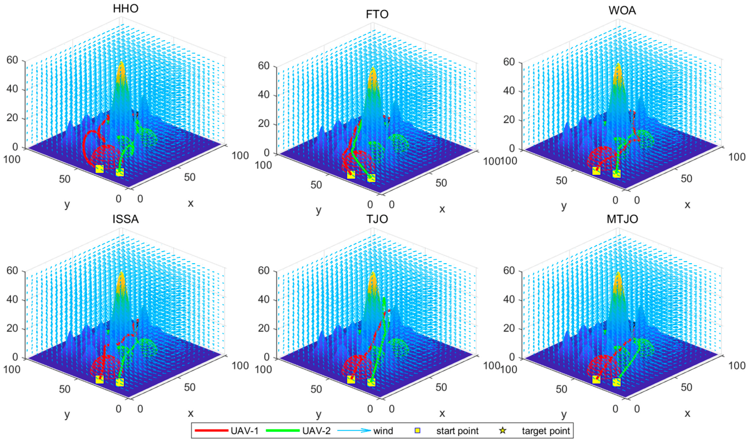
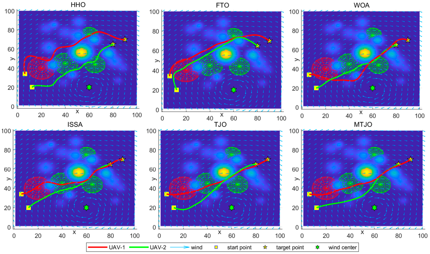
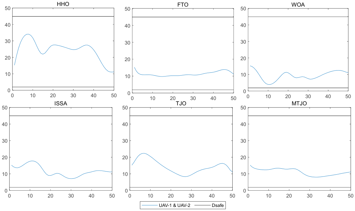
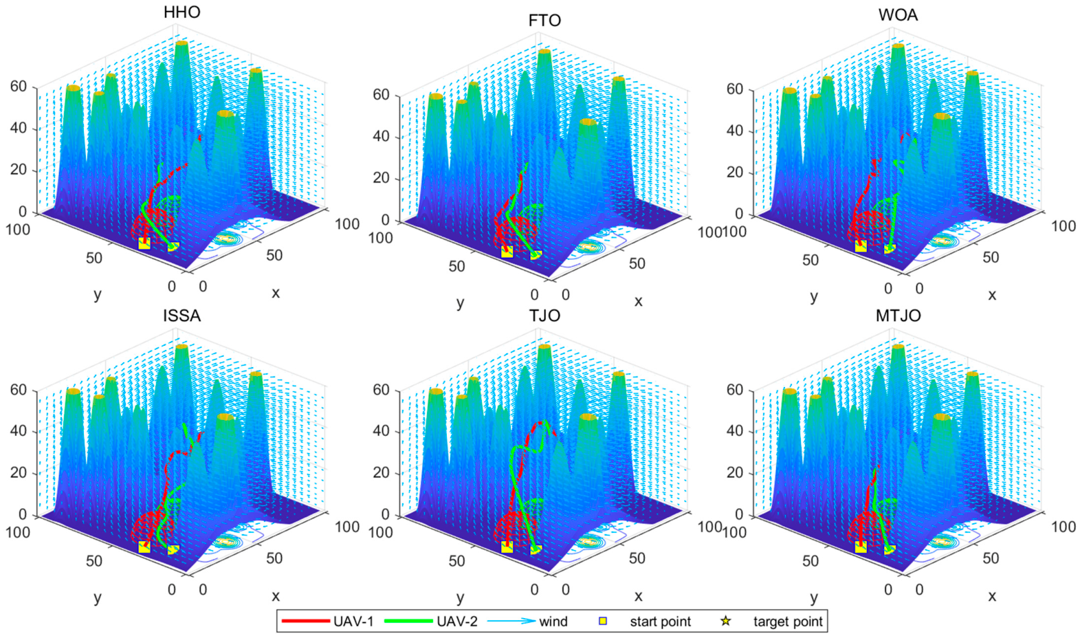
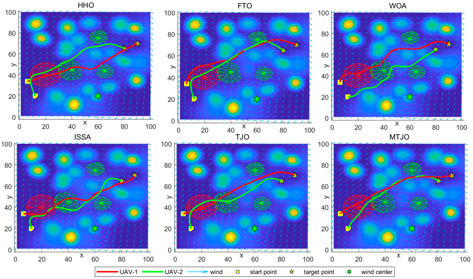
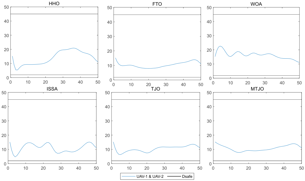
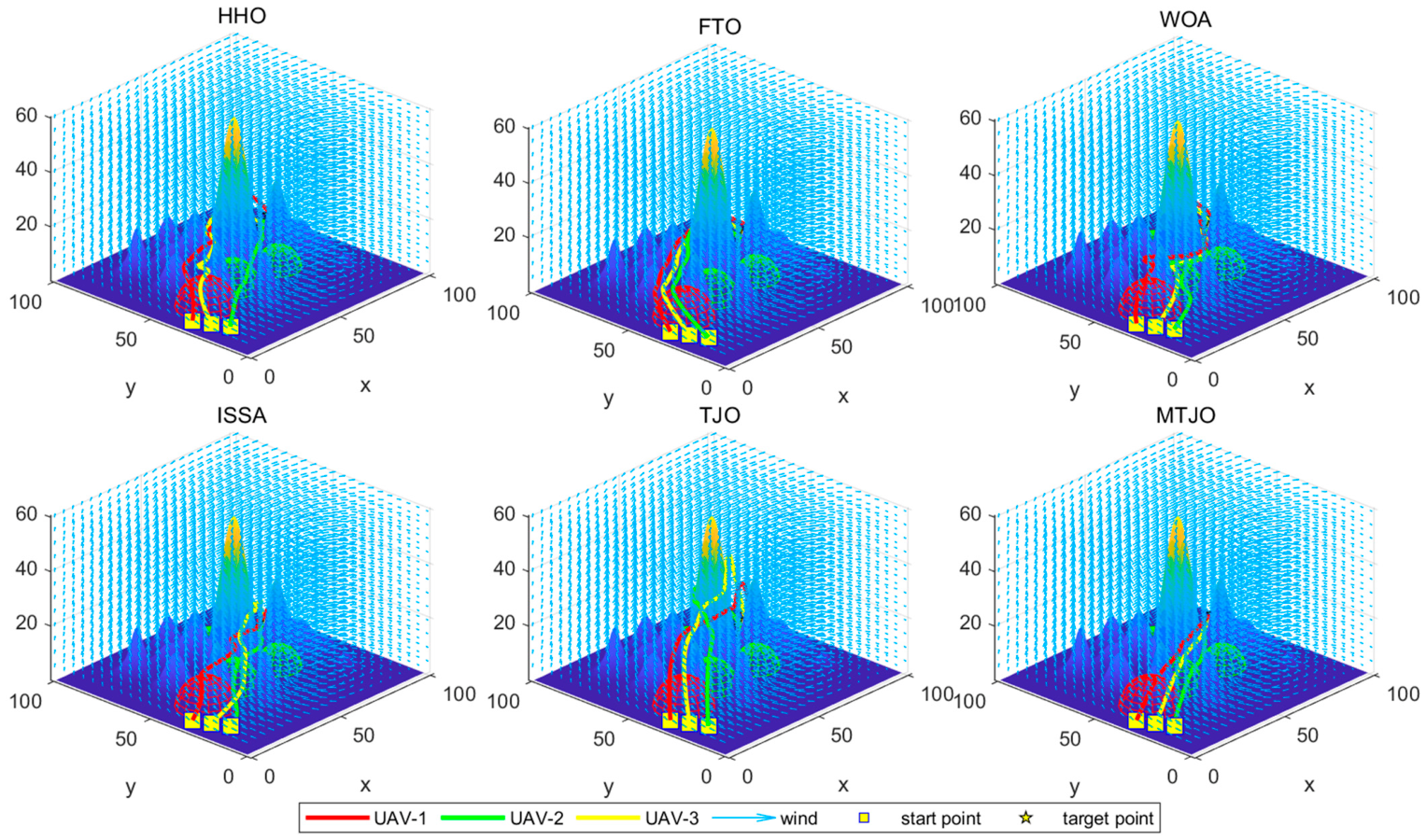
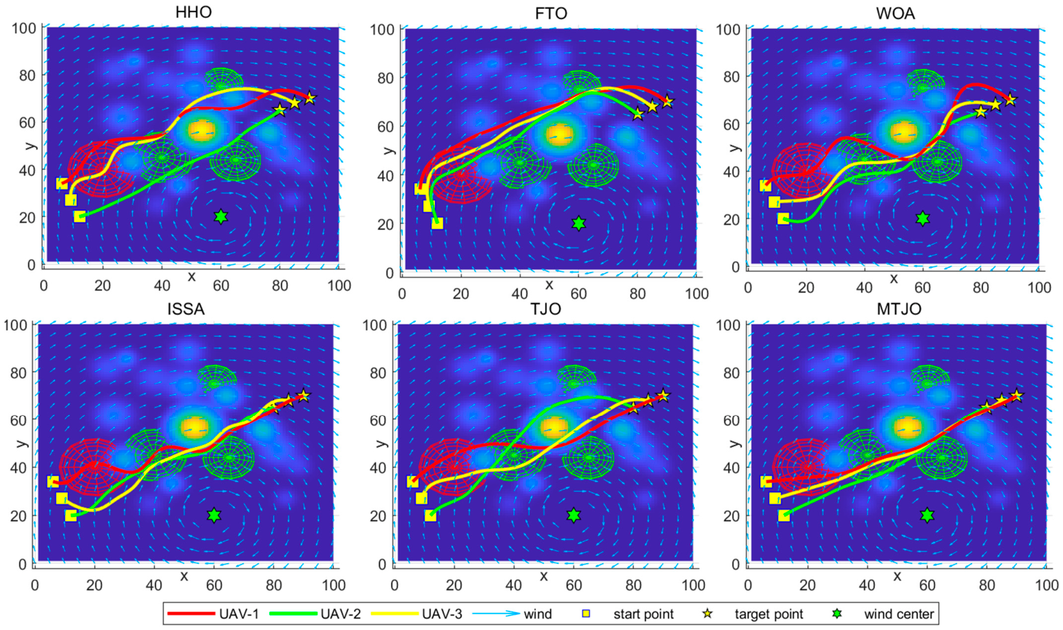
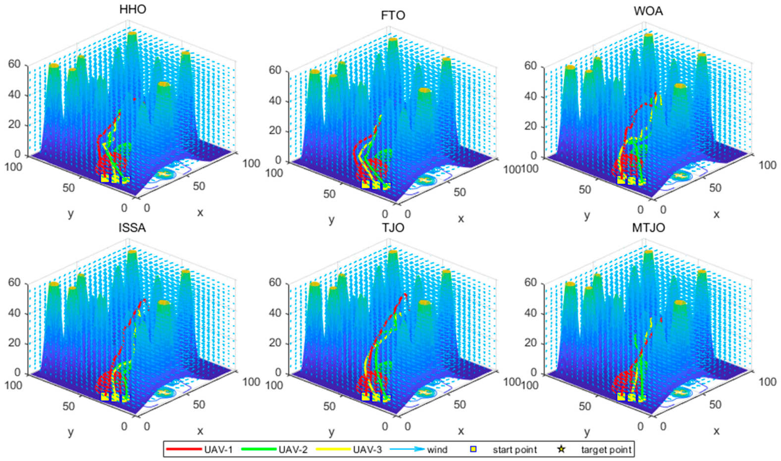
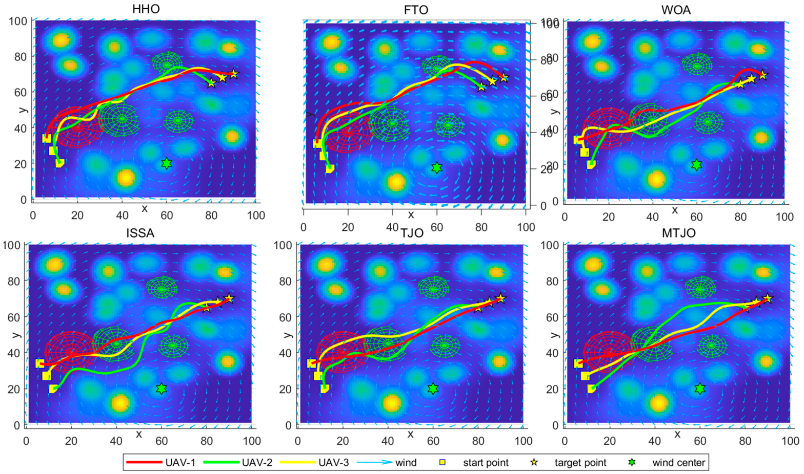
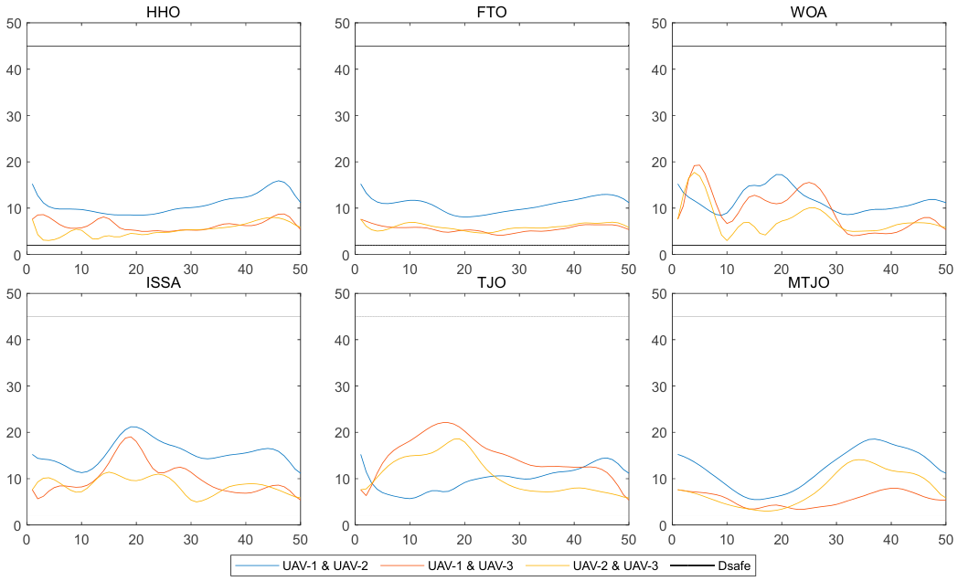
The 3D path results Figure 10 and top-view trajectories. Figure 11 show that the paths generated by MTJO can effectively avoid island terrain and restricted fly zones while maintaining smooth and compact shapes. Compared with several comparison algorithms, MTJO produces paths with smaller detours and more reasonable passages between complex terrain and risk regions. The inter-UAV distance curves further confirm that the distance between the two UAVs remains within the predefined safety and communication range during flight.
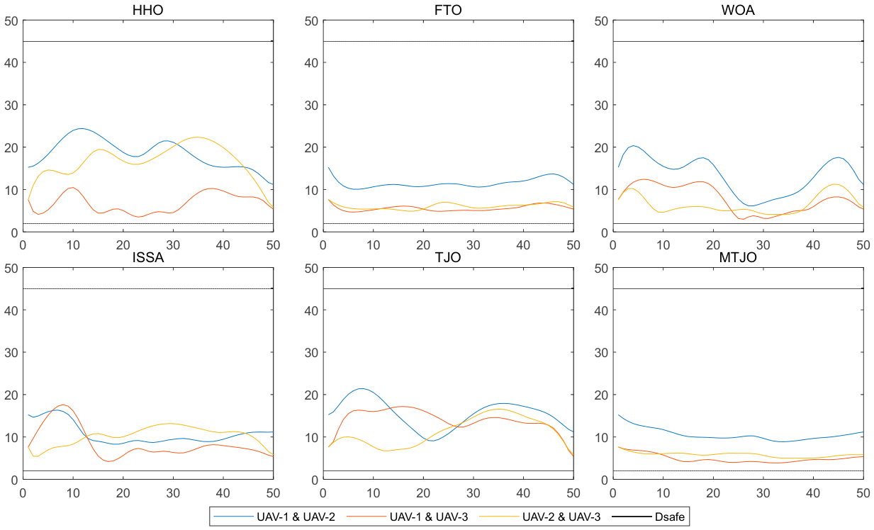
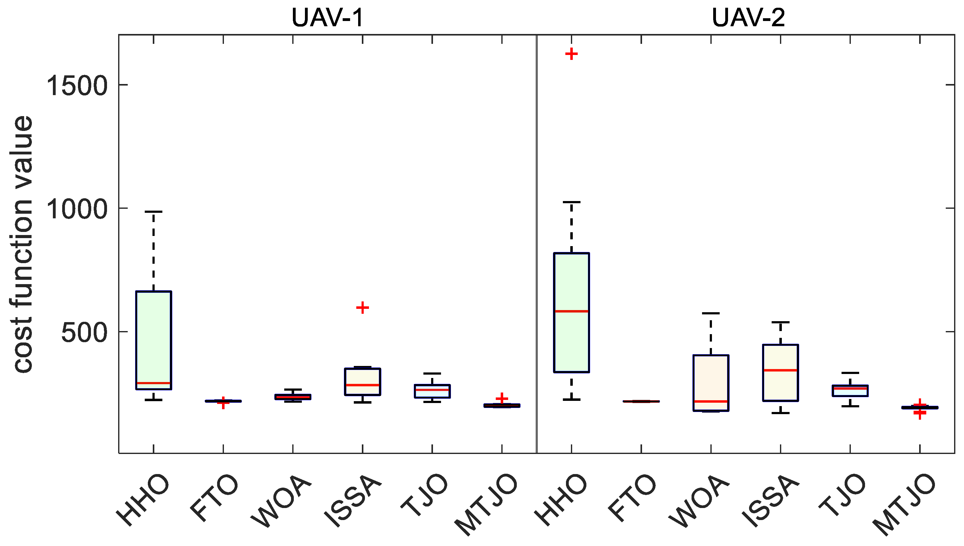
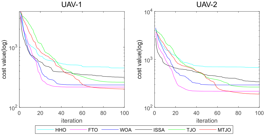
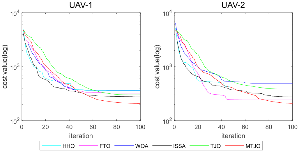
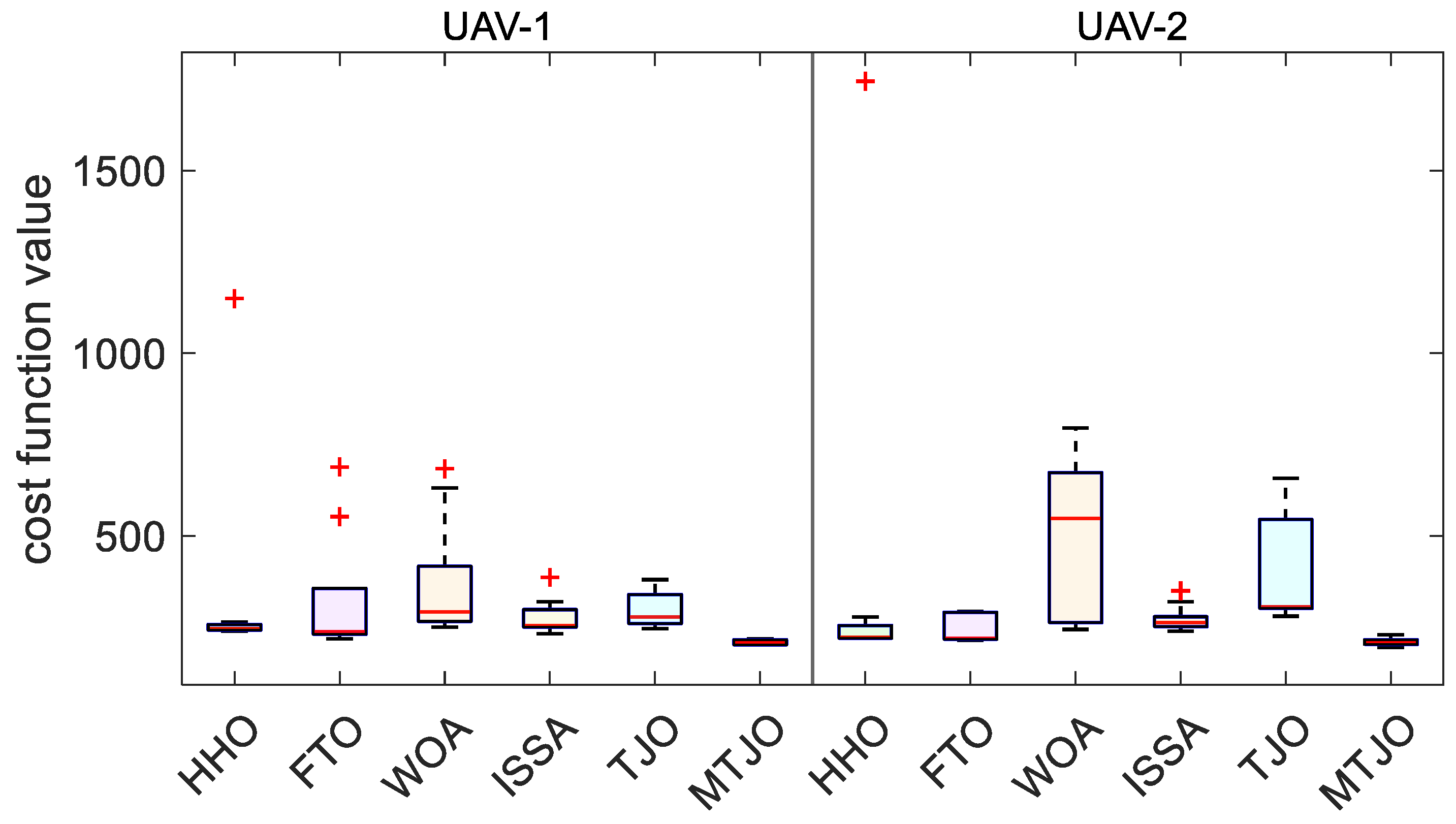
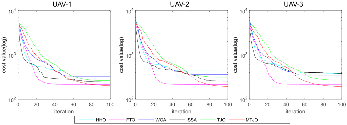
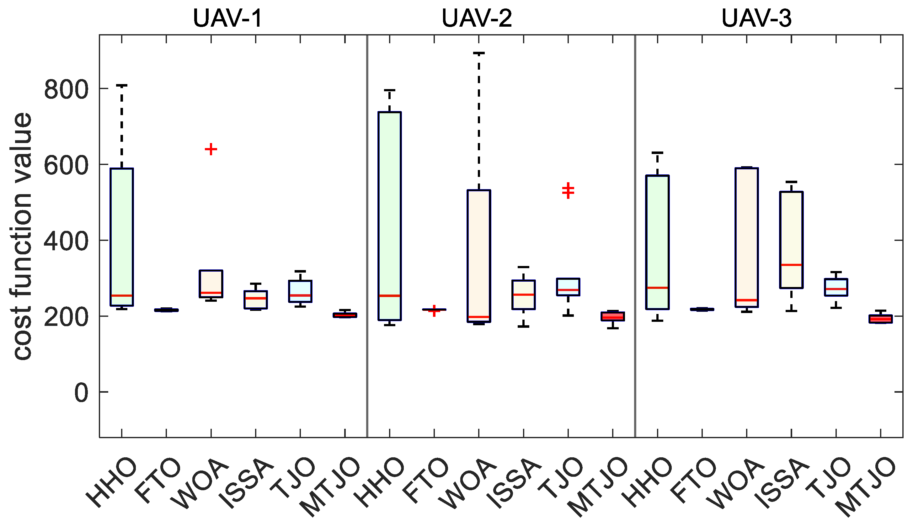
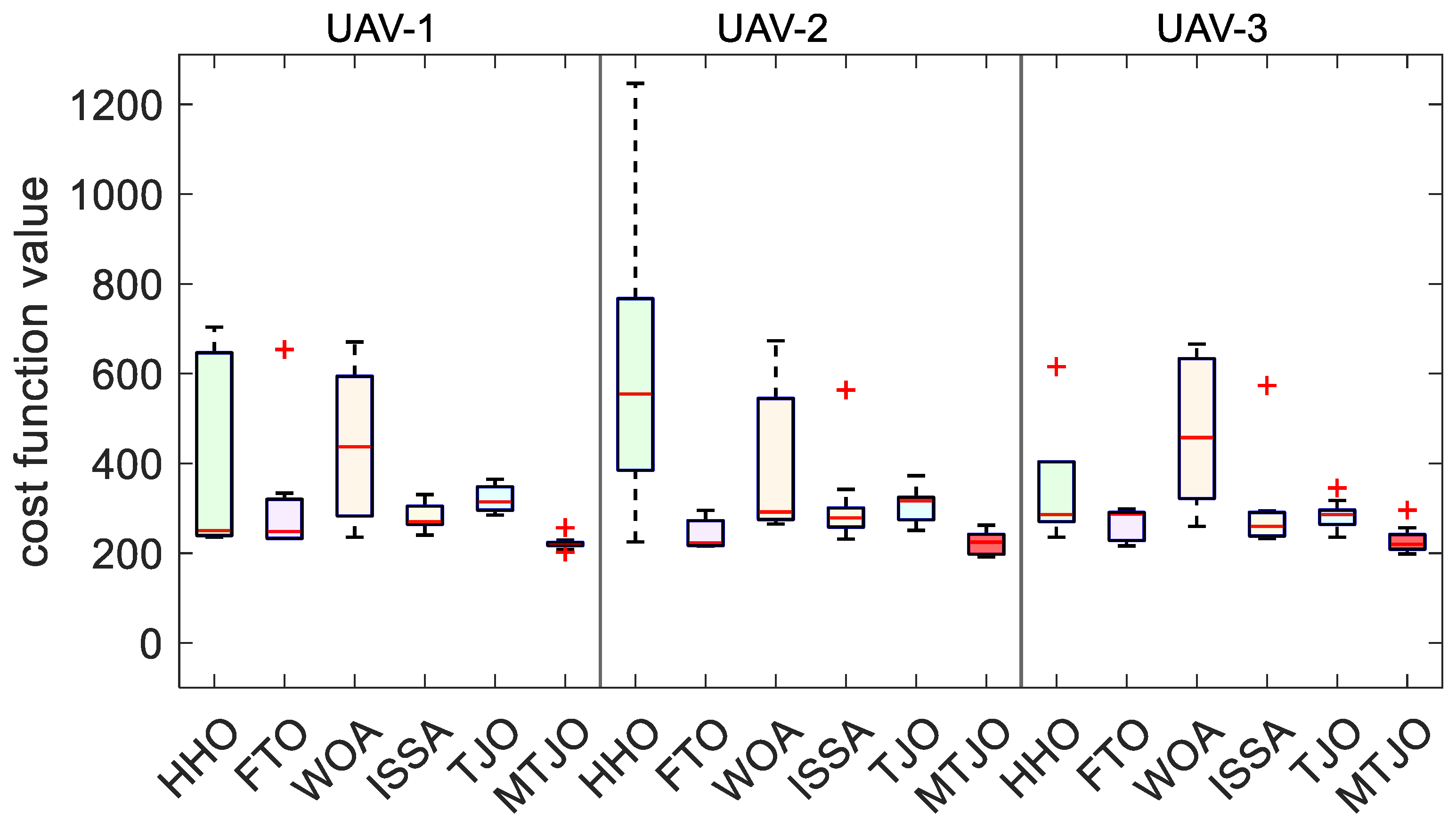
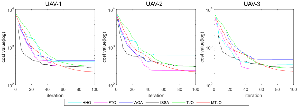
To further evaluate the cooperative safety, statistical stability, and convergence performance of different algorithms, the inter-UAV distance variation, path-cost distribution over 10 independent runs, and convergence curves are shown in Figure 12, Figure 13 and Figure 14, respectively.
The boxplots show that the cost values obtained by MTJO are more concentrated, with fewer large fluctuations, demonstrating better robustness. The convergence curves indicate that MTJO can rapidly reduce the cost value during iteration and maintain good exploitation ability in the later stage, finally achieving a lower convergence result than the comparison algorithms. These results verify that the proposed risk-opposition collaborative guidance, geometric multiscale adaptive mutation, and GQI decision-vector reconfiguration strategies can effectively improve the search accuracy and stability of MTJO in complex offshore path planning.
(2)
Scenarios 2
Compared with Scenario 1, this scenario contains a more complex island terrain distribution, where multiple terrain peaks and restricted fly zones jointly increase the difficulty of path search. Table 7 reports the statistical results of 10 independent runs.
As shown in Table 7, MTJO achieves the lowest mean cost for both UAVs. For UAV-1, the mean cost of MTJO is 208.9553, which is reduced by 41.93%, 35.63%, 43.12%, 24.21%, and 30.44% compared with HHO, FTO, WOA, ISSA, and TJO, respectively. For UAV-2, MTJO obtains a mean cost of 209.4155, reducing the cost by 50.08%, 13.63%, 57.59%, 23.77%, and 45.80%, respectively. Moreover, the standard deviations of MTJO are 7.5331 and 11.0336 for UAV-1 and UAV-2, respectively, which are much lower than those of most comparison algorithms. This indicates that MTJO maintains good stability and robustness in complex terrain environments. The corresponding UAV path lengths and synchronized flight times are reported in Table 8.
For a more comprehensive evaluation of the planning results, Figure 15, Figure 16, Figure 17, Figure 18 and Figure 19 present the best path obtained from 10 independent runs, the corresponding top-view trajectory, the convergence curves, the inter-UAV distance variation, and the path-cost distribution, respectively.
The 3D path results and top-view trajectories show that MTJO generates smoother and more compact paths while effectively avoiding island terrain and restricted fly zones. Compared with HHO, WOA, and TJO, the trajectories planned by MTJO contain fewer unnecessary detours and maintain a more reasonable spatial distribution between complex terrain and high-risk regions. This indicates that MTJO can better balance path length, terrain avoidance, and restricted-zone risk.
The inter-UAV distance curves confirm that the two UAVs remain within the predefined safety and communication range throughout the flight, avoiding collision risks while maintaining communication connectivity. The boxplots further show that MTJO has a more concentrated cost distribution, indicating stronger robustness over 10 independent runs.
The convergence curves show that MTJO decreases the cost efficiently and finally converges to a lower cost level than the comparison algorithms. Compared with TJO, MTJO maintains better late-stage optimization ability, indicating that the proposed strategies improve convergence performance and final solution quality.

5.2.2. Three UAVs Case

(1)
Scenarios 1
In the three-UAV case of Scenario 1, the cooperative path-planning ability of MTJO is further evaluated when the number of UAVs increases. Table 9 reports the statistical results of 10 independent runs, and Table 10 presents the corresponding path lengths and synchronized flight time.
As shown in Table 9, MTJO achieves the lowest mean cost for all three UAVs. The mean costs of MTJO for UAV-1, UAV-2, and UAV-3 are 203.1640, 194.8208, and 193.5473, respectively, which are reduced by 23.12%, 38.12%, and 29.15% compared with the original TJO. Compared with FTO, MTJO also reduces the mean costs by 6.00%, 10.10%, and 11.06%, respectively. In addition, the standard deviations of MTJO are 5.8519, 15.6919, and 11.4825, indicating good stability in the three-UAV cooperative planning task.
Table 10 shows that the path lengths obtained by MTJO are 99.8988 km, 84.0003 km, and 91.2155 km, which are the shortest among all algorithms. The corresponding synchronized flight time is 1.6650 h, also shorter than those of the comparison algorithms. This indicates that MTJO can reduce path length and improve task efficiency even when the number of UAVs increases.
The best 3D path, the corresponding top-view trajectory, the inter-UAV distance variation, the convergence curves, and the path-cost distribution over 10 independent runs are presented in Figure 20, Figure 21, Figure 22, Figure 23 and Figure 24, respectively.
The 3D path results and top-view trajectories show that MTJO generates feasible paths for all three UAVs while avoiding island terrain and restricted fly zones. Compared with several comparison algorithms, MTJO produces smaller detours and clearer cooperative trajectory patterns, demonstrating its ability to balance single-UAV path quality and multi-UAV cooperation.
The inter-UAV distance curves indicate that MTJO maintains reasonable distances among all UAV pairs, avoiding collision risks while preserving communication connectivity. The boxplots show that MTJO has a relatively concentrated cost distribution with small fluctuations, confirming its robustness in multi-UAV cooperative tasks. The convergence curves further show that MTJO finally reaches a lower cost level, verifying the effectiveness of the proposed improvement strategies.
(2)
Scenarios 2
In the three-UAV case of Scenario 2, a more complex offshore terrain is used to evaluate the planning performance of MTJO under complex terrain and multi-UAV cooperation. Compared with the two-UAV case, this experiment introduces stronger coupling among multiple trajectories, since each UAV must avoid environmental risks while maintaining feasible distances from the other two UAVs. Table 11 reports the statistical results of 10 independent runs, and Table 12 presents the corresponding path lengths and synchronized flight time.
As shown in Table 11, MTJO achieves the lowest mean cost for all three UAVs. The mean costs of MTJO for UAV-1, UAV-2, and UAV-3 are 221.1090, 222.7746, and 229.3360, respectively, which are reduced by 31.13%, 28.34%, and 19.29% compared with the original TJO. Compared with FTO, MTJO also reduces the mean costs by 30.10%, 7.18%, and 12.75%, respectively. In addition, the standard deviations of MTJO are 14.6182, 24.2719, and 29.5437, which are lower than those of most comparison algorithms. This indicates that MTJO can maintain stable optimization performance even when the number of UAVs and cooperative constraints increase.
Table 12 shows that MTJO obtains the shortest paths for all three UAVs, with path lengths of 109.9354 km, 98.7708 km, and 106.3718 km. The corresponding synchronized flight time is 1.8323 h, which is shorter than those of all comparison algorithms. This result indicates that MTJO not only reduces the comprehensive path cost but also improves the overall execution efficiency of the multi-UAV mission. Therefore, the proposed method is able to generate efficient cooperative paths under both environmental and inter-UAV constraints.
The best 3D path, the corresponding top-view trajectory, the inter-UAV distance variation, the path-cost distribution over 10 independent runs, and the convergence curves are presented in Figure 25, Figure 26, Figure 27, Figure 28 and Figure 29, respectively.
The 3D path results and top-view trajectories show that MTJO generates feasible paths for the three UAVs while avoiding island terrain and restricted fly zones. Compared with HHO, WOA, and TJO, MTJO produces fewer detours and more reasonable trajectory distributions, indicating better terrain and restricted-zone avoidance. Meanwhile, the three trajectories remain spatially coordinated, showing that MTJO can balance single-UAV path quality and multi-UAV cooperation.
The inter-UAV distance curves indicate that MTJO maintains feasible distances among all UAV pairs, avoiding collision risks while preserving communication connectivity. The boxplots show a concentrated cost distribution, demonstrating good robustness over 10 independent runs. The convergence curves further show that MTJO converges to a lower cost level, verifying the effectiveness of the proposed strategies in complex three-UAV cooperative path planning.

5.2.3. Statistical Significance Analysis

Because metaheuristic optimization algorithms are inherently stochastic, Mean and Std alone are insufficient to determine whether the performance differences between algorithms are statistically significant. Therefore, the Wilcoxon signed-rank test was employed to compare MTJO with HHO, FTO, WOA, ISSA, and TJO based on multiple independent runs. This nonparametric test does not require the samples to follow a normal distribution and is suitable for paired optimization results. The test used the same data protocol as the descriptive statistics, with valid paired samples constructed according to identical independent run indices. The significance level was set to 0.05, and the results are presented in Table 13. The p-value indicates whether a difference is statistically significant, whereas its direction should be interpreted together with the Mean, Std, and convergence results.
In 2UAV Scenario 1, the mean fitness values obtained by MTJO for UAV-1 and UAV-2 were 202.2907 and 189.7514, respectively, resulting in an aggregate mean fitness of 392.0421. This value was lower than the corresponding aggregate means of HHO, FTO, WOA, ISSA, and TJO, which were 1127.8536, 434.5220, 529.9355, 658.7181, and 528.3511, respectively. The p-values for the comparisons between MTJO and these algorithms were 0.0039, 0.0020, 0.0156, 0.0078, and 0.0020, all below 0.05. Therefore, the differences between MTJO and all comparison algorithms were statistically significant. Moreover, the Std values of MTJO for the two UAVs were 9.9122 and 10.6126, respectively, which were substantially lower than those of HHO, WOA, ISSA, and TJO, indicating good stability.
In 2UAV Scenario 2, the mean fitness values of MTJO for the two UAVs were 208.9553 and 209.4155, yielding an aggregate mean of 418.3708. In comparison, the aggregate means of HHO, FTO, WOA, ISSA, and TJO were 779.3522, 567.0924, 861.2010, 550.4048, and 686.7523, respectively. MTJO reduced the aggregate mean by 46.32%, 26.23%, 51.42%, 23.99%, and 39.08% relative to these algorithms. The corresponding p-values were 0.0078, 0.0039, 0.0039, 0.0020, and 0.0020, all below the significance threshold. The Std values of MTJO were only 7.5331 and 11.0336, lower than those of all comparison algorithms, demonstrating both high solution quality and stability in this scenario.
In 3UAV Scenario 1, MTJO achieved mean fitness values of 203.1640, 194.8208, and 193.5473 for the three UAVs, respectively, resulting in an aggregate mean of 591.5321. The corresponding aggregate means of HHO, FTO, WOA, ISSA, and TJO were 1196.5701, 650.4713, 1043.3630, 880.8982, and 852.2685, respectively. Even compared with FTO, which obtained the closest aggregate mean, MTJO achieved a reduction of 9.06%. The p-values for the five comparisons were 0.0156, 0.0020, 0.0313, 0.0078, and 0.0020, all below 0.05. This indicates that the performance improvements of MTJO remained statistically significant as the number of UAVs and cooperative constraints increased. The Std values of MTJO were lower than those of HHO, WOA, ISSA, and TJO, although higher than those of FTO. Therefore, the primary advantage of MTJO in this scenario was its lower fitness and favorable overall stability.
In 3UAV Scenario 2, the mean fitness values obtained by MTJO were 221.1090, 222.7746, and 229.3360, resulting in an aggregate mean of 673.2196. The aggregate means of HHO, FTO, WOA, ISSA, and TJO were 1376.0321, 819.1718, 1319.4928, 879.4952, and 916.1004, respectively. MTJO reduced the aggregate mean by 51.08%, 17.82%, 48.98%, 23.45%, and 26.51% relative to these algorithms. The p-values for the comparisons with FTO, WOA, ISSA, and TJO were 0.0313, 0.0156, 0.0020, and 0.0020, respectively, all below 0.05 and consistent with the trends observed in the descriptive statistics.
The p-value for the comparison between MTJO and HHO in this scenario was 0.0625, which did not reach the 0.05 significance level. This indicates that the available paired samples did not provide sufficient evidence of a statistically significant difference between the two algorithms at the 0.05 level. However, a nonsignificant result does not imply equivalent performance. The aggregate mean of MTJO was 673.2196, considerably lower than the HHO value of 1376.0321. In addition, the Std values of MTJO for the three UAVs were 14.6182, 24.2719, and 29.5437, compared with 233.5512, 382.9283, and 152.1914 for HHO. Therefore, the Mean, Std, and convergence results indicate that MTJO still achieved better overall solution quality and stability in this scenario, although its difference from HHO did not reach statistical significance at the 0.05 level.
Overall, 19 of the 20 pairwise comparisons produced p-values below 0.05. The Wilcoxon test results were generally consistent with the trends observed in the mean fitness, standard deviation, and convergence curves, providing further statistical support for the effectiveness and stability of MTJO in most scenarios. The single nonsignificant comparison also demonstrates that algorithm performance should be evaluated by jointly considering descriptive statistics, convergence behavior, and statistical tests rather than relying on a single p-value.

5.2.4. Ablation Study

To further verify the effectiveness of the proposed improvement strategies in MTJO, an ablation study was conducted in a representative high-complexity scenario. The original TJO was used as the baseline, and the three proposed strategies were gradually introduced, including the risk-opposition collaborative guidance strategy, the risk-based geometric multiscale adaptive mutation strategy, and the GQI-based decision-vector reconfiguration strategy. Accordingly, four algorithm variants were constructed: TJO, TJO+G, TJO+G+M, and the full MTJO. Here, TJO+G denotes TJO with only the risk-opposition guidance strategy, TJO+G+M denotes TJO with both the guidance and mutation strategies, and MTJO denotes the complete algorithm containing all three proposed strategies.
As shown in Table 14, the original TJO obtains a mean final total fitness of 686.75 with a standard deviation of 160.39, indicating relatively unstable search performance in the complex scenario. After introducing the risk-opposition collaborative guidance strategy, the mean final total fitness of TJO+G decreases to 524.39, corresponding to an improvement of 23.64% over TJO. This result indicates that the guidance strategy can effectively correct the global search direction by using high-risk region information. When the geometric multiscale adaptive mutation strategy is further added, the mean final total fitness decreases to 426.92, and the improvement over TJO increases to 37.83%. Meanwhile, the standard deviation is significantly reduced to 20.61, suggesting that the mutation strategy can effectively correct local high-risk trajectory segments and improve search stability.
The full MTJO achieves the lowest mean final total fitness of 418.37, with an improvement of 39.08% over the original TJO. Its standard deviation is further reduced to 12.86, indicating the best stability among all variants. Although the additional reduction brought by the GQI-based decision-vector reconfiguration strategy is relatively smaller in terms of mean fitness, it further narrows the distribution of final solutions and improves late-stage exploitation. The distribution of final total fitness and the corresponding mean and standard deviation for different ablation variants are presented in Figure 30 and Figure 31, respectively. The boxplot and Mean ± Std bar chart further show that, as the three strategies are progressively introduced, the final total fitness decreases and the result distribution becomes more concentrated. These results demonstrate that the three proposed strategies play complementary roles in global risk guidance, local trajectory correction, and late-stage refinement, jointly improving the optimization performance and robustness of MTJO in complex offshore multi-UAV path planning.

5.2.5. Parameter Sensitivity Analysis

To further explain the rationality of the control parameter settings in MTJO, a parameter sensitivity analysis was conducted in the two-UAV Scenario 2. As described above, compared with Scenario 1, Scenario 2 contains a more complex island terrain distribution, where multiple terrain peaks and restricted fly zones jointly increase the difficulty of path search. Therefore, this scenario was selected as a representative complex scenario to examine the influence of key parameter variations on the optimization performance and stability of MTJO. Four types of parameters were analyzed, including the risk-opposition guidance weight coefficient, high-risk individual ratio, fusion upper bound, and multiscale mutation scale coefficients. During the experiments, only the parameter under analysis was changed, while the other algorithm parameters, environmental settings, population size, maximum number of iterations, and path-encoding method remained unchanged.
Table 15 reports the statistical results of the final total fitness obtained by MTJO under different parameter settings in the two-UAV Scenario 2. Here, Mean and Std are calculated based on the sum of the final fitness values of the two UAVs, which reflects the overall optimization quality and stability of cooperative multi-UAV path planning.
As shown in Table 15, when the risk-opposition guidance weight coefficient is set to 0.09, the mean final total fitness is 439.80, with a standard deviation of 44.89. When this coefficient is increased to 0.27, the mean final total fitness rises to 458.81, and the standard deviation also increases to 53.20. In contrast, the default setting of 0.18 achieves a lower mean final total fitness of 418.37 and a smaller standard deviation of 12.86. This indicates that weak directional guidance is insufficient to fully utilize high-risk region information, whereas overly strong directional correction may disturb local convergence. The default coefficient provides a better balance between global risk avoidance and stable late-stage convergence.
For the high-risk individual ratio, when the ratio is set to 0.10, the mean final total fitness is 492.64, with a standard deviation of 157.05, indicating that insufficient extraction of high-risk region information weakens the effectiveness of risk-opposition guidance. When the ratio is increased to 0.40, the mean final total fitness decreases to 468.42, but the standard deviation remains high at 126.79, suggesting that too many low-quality individuals may introduce redundant or noisy information. The default ratio of 0.25 achieves the lowest mean final total fitness and the smallest fluctuation, indicating that it can effectively extract high-risk search-region information while avoiding excessive invalid guidance.
For the fusion upper bound, when it is set to 0.05, the mean final total fitness is 477.59 and the standard deviation is 116.70, indicating that the influence of the risk-guidance term is insufficient. When it is increased to 0.15, the mean final total fitness decreases to 431.70, but the standard deviation is still higher than that of the default setting. The default fusion upper bound of 0.10 achieves the lowest mean and standard deviation, indicating that this value can effectively control the influence of the risk-guidance term on candidate solution updates and prevent excessive perturbation from weakening population stability.
For the multiscale mutation scale coefficients, the smaller scale combination [0.01, 0.03, 0.08] obtains a mean final total fitness of 426.74 and a standard deviation of 24.81. Its overall performance is close to the default setting, but its ability to escape local regions is relatively weaker. When the larger scale combination [0.04, 0.08, 0.18] is used, the mean final total fitness increases to 478.33, and the standard deviation increases to 121.27, indicating that excessive local perturbation reduces the stability of path correction. The default scale combination [0.02, 0.06, 0.14] achieves the lowest mean final total fitness and the smallest standard deviation, suggesting that it provides a better balance between fine local path correction and moderate exploration.
Overall, the default parameter combination shows better average performance and stability in the two-UAV Scenario 2, indicating that MTJO has good robustness to perturbations in key parameters. It should be noted that all preceding comparison experiments, statistical significance analysis, and ablation experiments used the same fixed parameter settings, without scenario-specific parameter tuning, thereby ensuring the consistency and fairness of the experimental results.

5.3. Analysis of Algorithm Scalability

The scalability of the algorithm is an important indicator for evaluating its applicability to different path-planning tasks. In this paper, the scalability of the proposed MTJO is mainly analyzed from two aspects: different numbers of UAVs and different offshore environments.
The comparative results for the two-UAV and three-UAV cases show that MTJO can handle cooperative path planning problems with different fleet sizes. Even when the number of UAVs increases from two to three, the proposed algorithm still produces feasible trajectories while meeting terrain-avoidance, restricted-zone-avoidance, safety-distance, and communication-distance requirements. In both scenarios, MTJO also preserves competitive path quality and stable convergence behavior, which confirms its adaptability to larger cooperative UAV groups.
In addition, the experimental results under different offshore terrain settings demonstrate that MTJO can handle path-planning problems with different environmental risk distributions. The planned paths can effectively avoid island terrain and restricted fly zones while maintaining multi-UAV cooperative feasibility. Therefore, the comparative results verify that MTJO has good scalability and can be extended to multi-UAV cooperative path-planning tasks in complex offshore environments.

5.4. Discussion

This study investigates the cooperative path-planning problem for multiple UAVs in complex offshore environments, with particular attention to the ability of optimization algorithms to generate safe, smooth, and cooperative trajectories under multiple risk constraints. Although path planning for unmanned systems has been widely investigated, offshore path planning that simultaneously considers marine wind fields, island terrain, restricted fly zones, and multi-UAV cooperative constraints still requires further improvement in risk awareness and local refinement capability.
In this work, a three-dimensional offshore environment model is first constructed, including wind field disturbance, restricted fly zones, and island terrain. UAV performance constraints, multi-UAV cooperative constraints, and a comprehensive cost function are then established. Based on this framework, an improved MTJO algorithm is proposed to address the limitations of the original TJO in complex constrained path planning, such as insufficient risk awareness and local stagnation. The proposed MTJO enhances path optimization from three aspects: global search guidance, local path correction, and late-stage exploitation, through risk-opposition collaborative guidance, risk-based geometric multiscale adaptive mutation, and GQI decision-vector reconfiguration.
The experimental results show that MTJO can generate feasible cooperative trajectories in both two-UAV and three-UAV scenarios. Compared with the selected algorithms, MTJO achieves better performance in most statistical indicators, path length, synchronized flight time, and convergence behavior. In particular, in scenarios involving complex terrain and restricted regions, MTJO maintains compact and stable trajectories, indicating that the proposed risk-aware improvement strategies can effectively enhance the adaptability of the algorithm to complex offshore path planning. In addition, the scalability analysis shows that MTJO can maintain stable planning performance when the number of UAVs increases and the environmental terrain changes.
It should be noted that the current experiments are still based on simulation environments, where wind fields, terrain, and restricted fly zones are described using mathematical models. Dynamic factors in real offshore missions, such as time-varying wind fields, moving obstacles, communication delay, and sudden mission changes, have not been fully considered. These issues indicate that the current results should be interpreted as simulation-based validation under controlled offshore conditions, rather than complete real-world deployment verification.
Although the proposed MTJO shows promising performance in the above simulation experiments, this study still has several limitations. First, all experiments were conducted in MATLAB-based simulation environments, and hardware-in-the-loop or real-flight validation was not included. Therefore, the reported results mainly demonstrate the feasibility and comparative performance of MTJO under controlled simulation conditions. Second, the no-fly zones, island terrain, and hazardous regions were fixed during each independent simulation run to ensure fair comparisons among different algorithms. However, their locations, sizes, and risk coefficients are configurable and were adjusted across different scenarios to represent different levels of environmental complexity. Third, the marine wind field was simulated using the Lamb-Oseen model, and the island terrain was generated using a mixed Gaussian surface. These models provide controllable offshore test environments but do not fully represent real-time ocean meteorological data or high-resolution geographic information. Finally, this study did not explicitly consider time-varying no-fly zones, dynamically evolving hazardous areas, sensor errors, communication delays, or flight-control tracking errors. These factors are beyond the scope of the current model and should be considered when extending the proposed method to practical offshore emergency missions.
The cooperation considered in this study is defined at the cooperative path-planning level. Specifically, the proposed framework assumes that the mission targets of each UAV are given in advance and focuses on generating feasible and risk-aware trajectories that satisfy inter-UAV safety-distance, communication-distance, and synchronized-arrival constraints. Therefore, this work does not address higher-level cooperative mission functions such as task allocation, cooperative sensing, communication-topology optimization, network disconnection, or communication-failure recovery. These problems are usually studied in multi-UAV mission planning, sensing-and-communication co-design, or networked control frameworks, and require additional models for task utility, sensing coverage, information exchange, communication links, and online replanning. In the present work, communication is represented by a distance-based connectivity constraint, and collision avoidance is considered through predefined inter-UAV safety separation during offline path planning. Dynamic collision avoidance and communication-failure handling are not explicitly modeled. These issues require additional task-assignment, sensing, communication, and online decision-making models, and are therefore beyond the scope of the present cooperative path-planning formulation.

6. Conclusions and Future Work

This paper investigates the multi-UAV cooperative path planning problem in complex offshore environments. To describe the environmental constraints in practical missions, a three-dimensional environment model is constructed, including marine wind disturbance, restricted fly zones, and island terrain. Based on this model, UAV performance constraints, multi-UAV cooperative constraints, and a comprehensive cost function are further established to evaluate the feasibility and quality of candidate trajectories.
To address the limited risk-awareness and local refinement ability of the original TJO in complex constrained path planning, an improved MTJO algorithm is proposed. First, a risk-opposition collaborative guidance strategy is designed to introduce high-risk individual information into the guidance process, enabling the population to move toward promising regions while avoiding unfavorable search areas. Second, a risk-based geometric multiscale adaptive mutation strategy is proposed to refine local path control blocks with high-risk or stagnation characteristics, thereby improving local obstacle avoidance, path smoothness, and cooperative feasibility. Finally, a GQI decision-vector reconfiguration strategy is introduced to further refine the current best solution when the algorithm stagnates or enters the later search stage. These strategies enhance the path-search ability of MTJO from global guidance, local correction, and late-stage exploitation.
Experimental results show that MTJO can generate smooth cooperative trajectories satisfying multiple constraints in different offshore scenarios. Compared with the selected algorithms, MTJO achieves better overall performance in path quality, convergence behavior, and constraint satisfaction, demonstrating its effectiveness for multi-UAV cooperative path planning in complex offshore environments.
Future work will focus on dynamic offshore environment modeling, including time-varying wind fields, moving obstacles, and dynamically evolving hazardous or emergency-response regions. Online replanning mechanisms will be further developed to improve the adaptability of the proposed method under uncertain mission conditions. In addition, hardware-in-the-loop simulations and real UAV flight experiments will be conducted to evaluate the practical applicability and robustness of MTJO. Broader multi-UAV cooperation issues, such as task allocation, adaptive sensing, dynamic obstacle avoidance, communication-topology constraints, and communication-failure recovery, will also be considered in future studies.

Author Contributions

Conceptualization, T.Z. and F.M.; methodology, T.Z. and F.M.; software, T.Z.; validation, F.M.; formal analysis, T.Z. investigation, F.M.; writing-original draft preparation, T.Z. and S.D.; writing-review and editing F.M.; visualization, T.Z. and S.D.; supervision, F.M.; funding acquisition, F.M. All authors have read and agreed to the published version of the manuscript.

Funding

This work was supported by the Engineering Research Center of Integration and Application of Digital Learning Technology, Ministry of Education (1411011).

Data Availability Statement

The original contributions presented in this study are included in the article. Further inquiries can be directed to the corresponding author.

Acknowledgments

The authors would like to thank the anonymous reviewers for their valuable comments.

Conflicts of Interest

The authors declare no conflict of interest.

References

  1. Husnain, A.U.; Mokhtar, N.; Shah, N.M.; Dahari, M.; Iwahashi, M. A Systematic Literature Review (SLR) on Autonomous Path Planning of Unmanned Aerial Vehicles. Drones 2023, 7, 118. [Google Scholar] [CrossRef]
  2. Rahman, M.; Sarkar, N.I.; Lutui, R. A Survey on Multi-UAV Path Planning: Classification, Algorithms, Open Research Problems, and Future Directions. Drones 2025, 9, 263. [Google Scholar] [CrossRef]
  3. Cho, S.W.; Park, H.J.; Lee, H.; Shim, D.H.; Kim, S.-Y. Coverage Path Planning for Multiple Unmanned Aerial Vehicles in Maritime Search and Rescue Operations. Comput. Ind. Eng. 2021, 161, 107612. [Google Scholar] [CrossRef]
  4. Sun, S.; Zhang, H.; Dong, E. Multi-UAV Path Planning Based on IACO and Improved YOLOV8 Perception for Maritime Search and Rescue. EURASIP J. Wirel. Commun. Netw. 2025, 2025, 94. [Google Scholar] [CrossRef]
  5. Jones, M.; Djahel, S.; Welsh, K. Path-Planning for Unmanned Aerial Vehicles with Environment Complexity Considerations: A Survey. ACM Comput. Surv. 2023, 55, 1–39. [Google Scholar] [CrossRef]
  6. Wu, P.; Xie, J.; Liu, Y.; Chen, J. Risk-Bounded and Fairness-Aware Path Planning for Urban Air Mobility Operations under Uncertainty. Aerosp. Sci. Technol. 2022, 127, 107738. [Google Scholar] [CrossRef]
  7. Li, H.; Miao, F.; Mei, X. Facilitating Multi-UAVs Application for Rescue in Complex 3D Sea Wind Offshore Environment: A Scalable Multi-UAVs Collaborative Path Planning Method Based on Improved Coatis Optimization Algorithm. Ocean Eng. 2025, 324, 120701. [Google Scholar] [CrossRef]
  8. Zhang, C.; Liu, Y.; Hu, C. Path Planning with Time Windows for Multiple UAVs Based on Gray Wolf Algorithm. Drones 2022, 6, 397. [Google Scholar] [CrossRef]
  9. Yang, Z.; Yu, X.; Dedman, S.; Rosso, M.; Zhu, J.; Yang, J.; Xia, Y.; Tian, Y.; Zhang, G.; Wang, J. UAV Remote Sensing Applications in Marine Monitoring: Knowledge Visualization and Review. Sci. Total Environ. 2022, 838, 155939. [Google Scholar] [CrossRef] [PubMed]
  10. Doukari, M.; Batsaris, M.; Papakonstantinou, A.; Topouzelis, K. A Protocol for Aerial Survey in Coastal Areas Using UAS. Remote Sens. 2019, 11, 1913. [Google Scholar] [CrossRef]
  11. Li, Y.; Chen, W.; Fu, B.; Wu, Z.; Hao, L. A Global Coverage Path Planning Method for Multi-UAV Maritime Surveillance in Complex Obstacle Environments. Drones 2024, 8, 764. [Google Scholar] [CrossRef]
  12. Kazemdehbashi, S.; Liu, Y. An Algorithm with Exact Bounds for Coverage Path Planning in UAV-Based Search and Rescue under Windy Conditions. Comput. Oper. Res. 2025, 173, 106822. [Google Scholar] [CrossRef]
  13. Miao, F.; Li, H.; Yan, G.; Mei, X.; Wu, Z.; Zhao, W.; Liu, T.; Zhang, H. Optimizing UAV Path Planning in Maritime Emergency Transportation: A Novel Multi-Strategy White Shark Optimizer. J. Mar. Sci. Eng. 2024, 12, 1207. [Google Scholar] [CrossRef]
  14. Miao, F.; Li, H.; Mei, X. Three-Dimensional Path Planning of UAVs for Offshore Rescue Based on a Modified Coati Optimization Algorithm. J. Mar. Sci. Eng. 2024, 12, 1676. [Google Scholar] [CrossRef]
  15. Yang, L.; Qi, J.; Song, D.; Xiao, J.; Han, J.; Xia, Y. FC-RRT*: An Improved Path Planning Algorithm for UAV in 3D Complex Environment. ISPRS Int. J. Geo-Inf. 2022, 11, 112. [Google Scholar] [CrossRef]
  16. Pang, B.; Hu, X.; Dai, W.; Low, K.H. UAV Path Optimization with an Integrated Cost Assessment Model Considering Third-Party Risks in Metropolitan Environments. Reliab. Eng. Syst. Saf. 2022, 222, 108399. [Google Scholar] [CrossRef]
  17. Tang, H.; Zhu, Q.; Qin, B.; Song, R.; Li, Z. UAV Path Planning Based on Third-Party Risk Modeling. Sci. Rep. 2023, 13, 22259. [Google Scholar] [CrossRef] [PubMed]
  18. Dijkstra, E.W. A Note on Two Problems in Connexion with Graphs. Numer. Math. 1959, 1, 269–271. [Google Scholar] [CrossRef]
  19. Hart, P.E.; Nilsson, N.J.; Raphael, B. A Formal Basis for the Heuristic Determination of Minimum Cost Paths. IEEE Trans. Syst. Sci. Cybern. 1968, 4, 100–107. [Google Scholar] [CrossRef]
  20. Karaman, S.; Frazzoli, E. Sampling-Based Algorithms for Optimal Motion Planning. Int. J. Robot. Res. 2011, 30, 846–894. [Google Scholar] [CrossRef]
  21. LaValle, S.M. Rapidly-Exploring Random Trees: A New Tool for Path Planning; Iowa State University: Ames, IA, USA, 1998. [Google Scholar]
  22. Jiang, Y.; Xu, X.-X.; Zheng, M.-Y.; Zhan, Z.-H. Evolutionary Computation for Unmanned Aerial Vehicle Path Planning: A Survey. Artif. Intell. Rev. 2024, 57, 267. [Google Scholar] [CrossRef]
  23. Yang, X.-S. Nature-Inspired Metaheuristic Algorithms, 2nd ed.; Luniver Press: Frome, UK, 2010. [Google Scholar]
  24. Kennedy, J.; Eberhart, R. Particle Swarm Optimization. In Proceedings of the ICNN’95—International Conference on Neural Networks; IEEE: Piscataway, NJ, USA, 1995; Volume 4, pp. 1942–1948. [Google Scholar]
  25. Mirjalili, S.; Mirjalili, S.M.; Lewis, A. Grey Wolf Optimizer. Adv. Eng. Softw. 2014, 69, 46–61. [Google Scholar] [CrossRef]
  26. Mirjalili, S.; Lewis, A. The Whale Optimization Algorithm. Adv. Eng. Softw. 2016, 95, 51–67. [Google Scholar] [CrossRef]
  27. Xue, J.; Shen, B. A Novel Swarm Intelligence Optimization Approach: Sparrow Search Algorithm. Syst. Sci. Control. Eng. 2020, 8, 22–34. [Google Scholar] [CrossRef]
  28. Wolpert, D.H.; Macready, W.G. No Free Lunch Theorems for Optimization. IEEE Trans. Evol. Comput. 1997, 1, 67–82. [Google Scholar] [CrossRef]
  29. Wang, J.; Shang, Z. Traffic Jam Optimizer: A Novel Swarm-Based Metaheuristic Algorithm for Solving Global Optimization Problems. Appl. Math. Model. 2026, 150, 116410. [Google Scholar] [CrossRef]
  30. Zhao, W.; Wang, L.; Zhang, Z.; Mirjalili, S.; Khodadadi, N.; Ge, Q. Quadratic Interpolation Optimization (QIO): A New Optimization Algorithm Based on Generalized Quadratic Interpolation and Its Applications to Real-World Engineering Problems. Comput. Methods Appl. Mech. Eng. 2023, 417, 116446. [Google Scholar] [CrossRef]
  31. Rai, R.; Sasmal, B.; Das, A.; Bharasa, T.; Dhal, K.G.; Naskar, P.K. Opposition Based Learning for Metaheuristic Algorithms: Theory, Variants, Applications, and Performance Evaluation. Swarm Evol. Comput. 2026, 100, 102271. [Google Scholar] [CrossRef]
  32. Rojas-Morales, N.; Riff, M.C.; Montero, E. A Survey and Classification of Opposition-Based Metaheuristics. Comput. Ind. Eng. 2017, 110, 424–435. [Google Scholar] [CrossRef]
  33. Gong, Y.; Zhang, S.; Luo, M.; Ma, S. A Mutation Operator Self-Adaptive Differential Evolution Particle Swarm Optimization Algorithm for USV Navigation. Front. Neurorobot. 2022, 16, 1076455. [Google Scholar] [CrossRef] [PubMed]
  34. Zhang, J.; Sanderson, A.C. JADE: Adaptive Differential Evolution With Optional External Archive. IEEE Trans. Evol. Comput. 2009, 13, 945–958. [Google Scholar] [CrossRef]
  35. Shen, Y.; Zhu, Y.; Kang, H.; Sun, X.; Chen, Q.; Wang, D. UAV Path Planning Based on Multi-Stage Constraint Optimization. Drones 2021, 5, 144. [Google Scholar] [CrossRef]
  36. Heidari, A.A.; Mirjalili, S.; Faris, H.; Aljarah, I.; Mafarja, M.; Chen, H. Harris Hawks Optimization: Algorithm and Applications. Future Gener. Comput. Syst. 2019, 97, 849–872. [Google Scholar] [CrossRef]
  37. Mirjalili, S.; Gandomi, A.H.; Mirjalili, S.M.; Saremi, S.; Faris, H.; Mirjalili, S.M. Salp Swarm Algorithm: A Bio-Inspired Optimizer for Engineering Design Problems. Adv. Eng. Softw. 2017, 114, 163–191. [Google Scholar] [CrossRef]
  38. Tudose, A.M.; Sidea, D.O.; Picioroaga, I.I.; Anton, N.; Bulac, C. Increasing Distributed Generation Hosting Capacity Based on a Sequential Optimization Approach Using an Improved Salp Swarm Algorithm. Mathematics 2024, 12, 48. [Google Scholar] [CrossRef]
  39. Saad, M.R.; Emam, M.M.; Hosney, M.E.; Samee, N.A.; Alkanhel, R.I.; Houssein, E.H. Fourier Transform Optimizer: A Novel Physics-Inspired Metaheuristic Algorithm for Optimization Problems. Knowl. Based Syst. 2026, 340, 115651. [Google Scholar] [CrossRef]
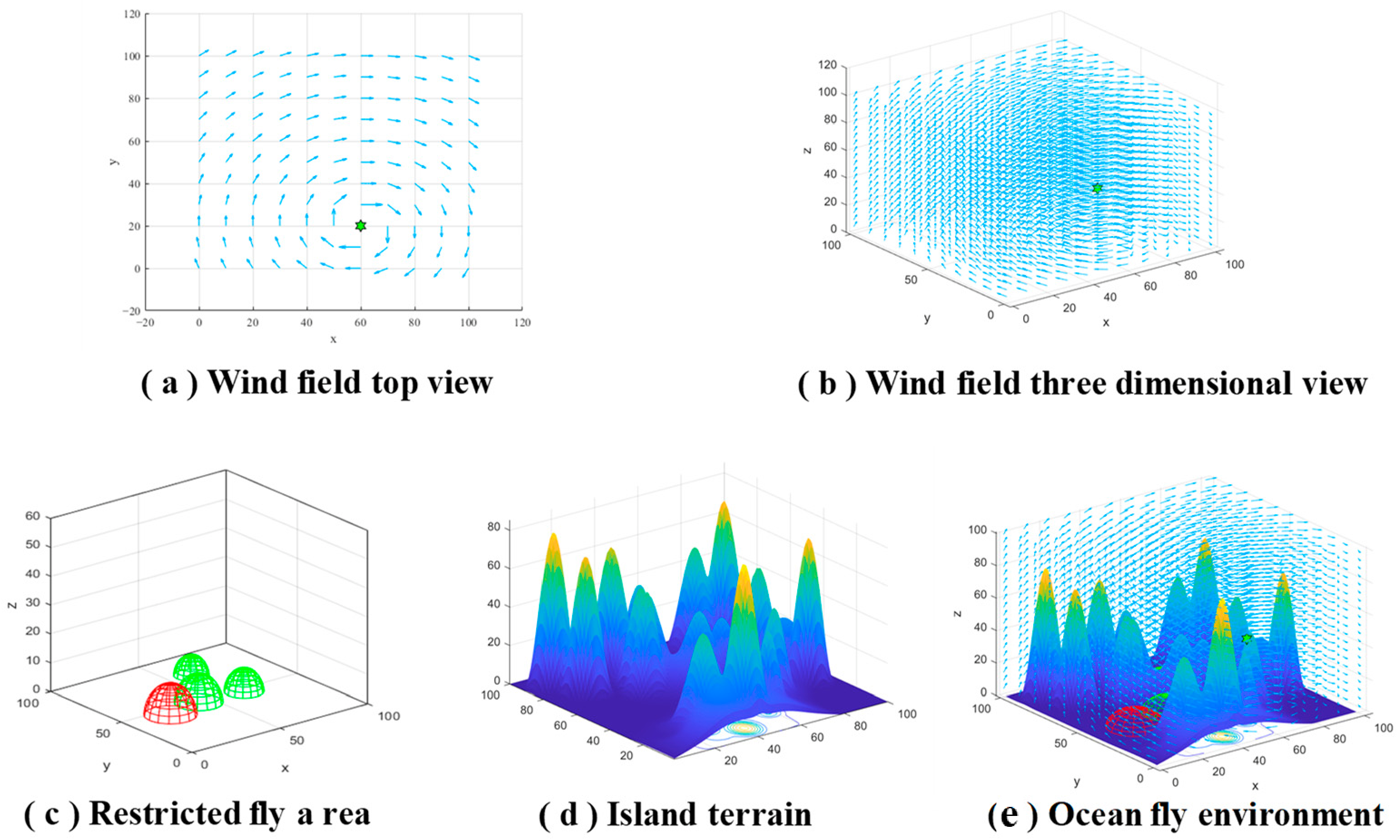
Figure 1. Schematic diagram of environment construction.
Jmse 14 01187 g001
Figure 2. Multi-UAVs path planning.
Jmse 14 01187 g002
Figure 3. Risk-Opposition Collaborative Guidance Strategy.
Jmse 14 01187 g003
Figure 4. Risk-Based Geometric Multiscale Adaptive Mutation Strategy.
Jmse 14 01187 g004
Figure 5. GQI Decision-Vector Reconfiguration Strategy.
Jmse 14 01187 g005
Figure 6. The principle of time judgement.
Jmse 14 01187 g006
Figure 7. The schematic diagram of sea wind cost.
Jmse 14 01187 g007
Figure 8. The principle of path planning.
Jmse 14 01187 g008
Figure 9. The principle of path planning.
Jmse 14 01187 g009
Figure 10. The graph of the minimum cost path after the algorithm runs 10 times.
Jmse 14 01187 g010
Figure 11. The minimum cost path graph in the top view after the algorithm runs 10 times.
Jmse 14 01187 g011
Figure 12. Distance between UAVs at the same moment.
Jmse 14 01187 g012
Figure 13. Box plot of the path cost from 10 independent runs.
Jmse 14 01187 g013
Figure 14. Convergence curves of optimization algorithms used in UAV path planning.
Jmse 14 01187 g014
Figure 15. The graph of the minimum cost path after the algorithm runs 10 times.
Jmse 14 01187 g015
Figure 16. The minimum cost path graph in the top view after the algorithm runs 10 times.
Jmse 14 01187 g016
Figure 17. Convergence curves of optimization algorithms used in UAV path planning.
Jmse 14 01187 g017
Figure 18. Distance between UAVs at the same moment.
Jmse 14 01187 g018
Figure 19. Box plot of the path cost from 10 independent runs.
Jmse 14 01187 g019
Figure 20. The graph of the minimum cost path after the algorithm runs 10 times.
Jmse 14 01187 g020
Figure 21. The minimum cost path graph in the top view after the algorithm runs 10 times.
Jmse 14 01187 g021
Figure 22. Distance between UAVs at the same moment.
Jmse 14 01187 g022
Figure 23. Convergence curves of optimization algorithms used in UAV path planning.
Jmse 14 01187 g023
Figure 24. Box plot of the path cost from 10 independent runs.
Jmse 14 01187 g024
Figure 25. The graph of the minimum cost path after the algorithm runs 10 times.
Jmse 14 01187 g025
Figure 26. The minimum cost path graph in the top view after the algorithm runs 10 times.
Jmse 14 01187 g026
Figure 27. Distance between UAVs at the same moment.
Jmse 14 01187 g027
Figure 28. Box plot of the path cost from 10 independent runs.
Jmse 14 01187 g028
Figure 29. Convergence curves of optimization algorithms used in UAV path planning.
Jmse 14 01187 g029
Figure 30. Distribution of final total fitness for different ablation variants.
Jmse 14 01187 g030
Figure 31. Mean and standard deviation of final total fitness for different ablation variants.
Jmse 14 01187 g031
Table 1. Algorithm Parameter Configurations.
AlgorithmParameter
WOAN = 100; D = 20; Tmax = 100
a is decreased from 2 to 0, b = 1, l ∈ [−1, 1]
HHON = 100; D = 20; Tmax = 100
E1 = 2(1 − t/Tmax); E0 ∈ [−1, 1];
q, r ∈ [0, 1]; J = 2(1 − rand); β = 1.5
FTON = 100; D = 20; Tmax = 100
β = 1.5 ,   α 0 = 0.1 ,   e l i t e r a t i o = 0.1
differential mixing factor = 0.5;
cutoff decreases from 0.9 to 0.1
ISSAN = 100; D = 20; Tmax = 100
p f o l l = 0.2 , p p i o n = 0.3
TJON = 100; D = 20; Tmax = 100
a t and c t decrease linearly from 2 to 0
MTJON = 100; D = 20; Tmax = 100
a t and c t decrease linearly from 2 to 0
high-risk ratio = 0.25;
w d i r = 0.18 1 t / T ;
fusion coefficient upper bound = 0.10;
initial mutation scales = 0.02, 0.06, 0.14;
maximum mutated blocks = 2;
GQI trigger: stall-count > 5 or t > 0.7T
Note: For fairness, all algorithms were configured with the same population size and maximum number of iterations, namely N = 100 and Tmax = 100. The remaining parameters listed for MTJO are algorithm-specific control parameters.
Table 2. Parameters of two UAVs.
AlgorithmParameterUAV-1UAV-2
Scenarios 1 and 2Initial position (km)(6, 34, 2)(12, 20, 2)
Destination position (km)(90, 70, 5)(80, 65, 5)
Speed range (km/h)(40 60)(40, 60)
Inter-UAV distance range (km)(3, 40)(3, 40)
Max heading-change angle (°)4545
Max climb angle (°)4545
Note: The same two-UAV parameter settings are used in Scenario 1 and Scenario 2.
Table 3. Parameters of three UAVs.
AlgorithmParameterUAV-1UAV-2UAV-3
Scenarios 1 and 2Initial position (km)(6, 34, 2)(12, 20, 2)(9, 27, 2)
Destination position (km)(90, 70, 5)(80, 65, 5)(85, 68, 5)
Speed range (km/h)(40 60)(40, 60)(40, 60)
Inter-UAV distance range (km)(3, 40)(3, 40)(3, 40)
Max heading-change angle (°)454545
Max climb angle (°)454545
Note: The same three-UAV parameter settings are used in Scenario 1 and Scenario 2.
Table 4. Environment Parameters.
CaseRestricted-Region Center (km)Restricted-Region Radius (km)Risk CoefficientVortex Center (km)Wind Intensity
Scenarios 1 and 2(20, 40, 0),
(65, 44, 0),
(40, 45, 0),
(60, 75, 0)
12, 9, 11, 812, 8, 10, 10(60, 20, z)100
Note: The same environmental settings, including restricted regions, vortex parameters, and wind intensity, are used in Scenario 1 and Scenario 2.
Table 5. Statistical results of fitness function values for each algorithm.
NoResultAlgorithms
HHOFTOWOAISSATJOMTJO
UAV-1Mean451.8261217.4331236.1122 316.5277 262.7171 202.2907
Std287.20382.557614.9613 115.6432 34.5123 9.9122
UAV-2Mean676.0275217.0889293.8233 342.1904 265.6340 189.7514
Std437.91650.8378171.1492 135.7944 39.9834 10.6126
Table 6. UAV path length and flight time.
NoResultAlgorithms
HHOFTOWOAISSATJOMTJO
UAV-1Path length (km)132.2876105.7673113.1862 106.3020 107.2537 97.2696
Flight time (h)2.20481.81581.8864 1.7717 2.0423 1.6212
UAV-2Path length (km)108.7691108.945790.4924 84.8375 122.5373 87.1438
Flight time (h)2.20481.81581.8864 1.7717 2.0423 1.6212
Note: 2 Identical flight times of UAV-1 and UAV-2 under the same algorithm are caused by the synchronized-arrival constraint.
Table 7. Statistical results of fitness function values for each algorithm.
NoResultAlgorithms
HHOFTOWOAISSATJOMTJO
UAV-1Mean359.8441324.6225367.3627275.6932300.3921208.9553
Std319.1279172.4993166.942546.754952.46467.5331
UAV-2Mean419.5081242.4699493.8383274.7116386.3602209.4155
Std535.736437.2448209.707334.247442.276011.0336
Table 8. UAV path length and flight time.
NoResultAlgorithms
HHOFTOWOAISSATJOMTJO
UAV-1Path length (km)120.1739108.9646124.7626126.8216129.7017100.8150
Flight time (h)2.00291.84562.07942.11372.32651.6803
UAV-2Path length (km)109.6385110.7344120.1645123.6671139.592297.3585
Flight time (h)2.00291.84562.07942.11372.32651.6803
Table 9. Statistical results of fitness function values for each algorithm.
NoResultAlgorithms
HHOFTOWOAISSATJOMTJO
UAV-1Mean386.7178216.1368328.9238 245.9655 264.2689 203.164
Std253.25562.5949154.9813 25.5164 35.1584 5.8519
UAV-2Mean433.9707216.7166364.1410 254.8948 314.8340 194.8208
Std287.35141.1715293.5089 52.4551 117.4633 15.6919
UAV-3Mean375.8816217.6179350.2982 380.0379 273.1656 193.5473
Std192.87971.8721186.9996 136.0789 29.8172 11.4825
Table 10. UAV path length and flight time.
NoResultAlgorithms
HHOFTOWOAISSATJOMTJO
UAV-1Path length (km)109.0479106.5609125.2674108.2392111.704399.8988
Flight time (h)1.81751.79762.08781.80402.15141.6650
UAV-2Path length (km)88.2368107.853192.407686.2966117.838084.0003
Flight time (h)1.81751.79762.08781.80402.15141.6650
UAV-3Path length (km)108.6029107.3412104.6932105.7938129.083891.2155
Flight time (h)1.81751.79762.08781.80402.15141.6650
Table 11. Statistical results of fitness function values for each algorithm.
NoResultAlgorithms
HHOFTOWOAISSATJOMTJO
UAV-1Mean411.4789316.3085442.6338 282.5836 321.0608 221.1090
Std233.5512153.2795176.9754 29.0910 29.3159 14.6182
UAV-2Mean614.2453240.011400.7939 306.3443 310.8654 222.7746
Std382.928335.7571167.8972 95.6705 38.0166 24.2719
UAV-3Mean350.3079262.8523476.0651 290.5673 284.1742 229.3360
Std152.191436.0481164.9023 102.1879 31.7363 29.5437
Table 12. UAV path length and flight time.
NoResultAlgorithms
HHOFTOWOAISSATJOMTJO
UAV-1Path length (km)120.3304117.1641137.7014132.3386142.0440109.9354
Flight time (h)2.00551.95272.29502.20562.36741.8323
UAV-2Path length (km)112.4525111.1187132.0893113.6326130.625098.7708
Flight time (h)2.00551.95272.29502.20562.36741.8323
UAV-3Path length (km)117.8065115.7196128.2692118.2849117.4317106.3718
Flight time (h)2.00551.95272.29502.20562.36741.8323
Table 13. Wilcoxon signed-rank test p-values between MTJO and comparison algorithms.
UAV
Number
ScenarioMTJO Against Other Algorithms
HHOFTOWOAISSATJO
2UAVScenarios 10.00390.00200.01560.00780.0020
Scenarios 20.00780.00390.00390.00200.0020
3UAVScenarios 10.01560.00200.03130.00780.0020
Scenarios 20.06250.03130.01560.00200.0020
Note: The values represent the p-values of the Wilcoxon signed-rank test between MTJO and each comparison algorithm. A p-value less than 0.05 indicates a statistically significant difference.
Table 14. Ablation study of MTJO in the high-complexity scenario.
VariantGuidanceMutationGQIMeanStdImprovement over TJO (%)
TJO×××686.75160.39
TJO+G××524.39143.4223.64
TJO+G+M×426.9220.6137.83
MTJO418.3712.8639.08
Note: √ indicates that the corresponding strategy is included, × indicates that it is not included.
Table 15. Parameter sensitivity analysis of MTJO in the two-UAV Scenario 2.
ParameterSettingMeanStd
Direction weight coefficient0.09439.8044.89
Direction weight coefficient0.18418.3712.86
Direction weight coefficient0.27458.8153.20
High-risk ratio0.10492.64157.05
High-risk ratio0.25418.3712.86
High-risk ratio0.40468.42126.79
Fusion upper bound0.05477.59116.70
Fusion upper bound0.10418.3712.86
Fusion upper bound0.15431.7036.79
Scale coefficients[0.01, 0.03, 0.08]426.7424.81
Scale coefficients[0.02, 0.06, 0.14]418.3712.86
Scale coefficients[0.04, 0.08, 0.18]478.33121.27
Disclaimer/Publisher’s Note: The statements, opinions and data contained in all publications are solely those of the individual author(s) and contributor(s) and not of MDPI and/or the editor(s). MDPI and/or the editor(s) disclaim responsibility for any injury to people or property resulting from any ideas, methods, instructions or products referred to in the content.