Article

The Labrador Coastal Current: Observations from Surface Drifters and Autonomous Gliders
by
Eric C. J. Oliver
1,* and
Clark Richards
1,2
1
Department of Oceanography, Dalhousie University, Halifax, NS B3H 4R2, Canada
2
Fisheries and Oceans Canada, Bedford Institute of Oceanography, Dartmouth, NS B2Y 4A2, Canada
*
Author to whom correspondence should be addressed.
J. Mar. Sci. Eng. 2026, 14(13), 1163; https://doi.org/10.3390/jmse14131163
Submission received: 14 April 2026 / Revised: 27 May 2026 / Accepted: 16 June 2026 / Published: 24 June 2026
(This article belongs to the Special Issue Marine Modelling and Environmental Statistics—2nd Edition)

Abstract

This study focuses on the Labrador Coastal Current (LCC), which is the coastal branch of the Labrador Current System (LCS). We characterize the LCS by combining existing Global Drifter Program (GDP) data with new surface drifters deployed by the Community-based Observations of Nunatsiavut Ocean Circulation (CONOC) project, specifically designed to fill the near-coast gap where the LCC lies. Autonomous ocean gliders are used to map hydrography and infer baroclinic and barotropic circulation components of the LCS. Tidal currents are generally weak across most of the shelf but are notably stronger in areas such as the Hudson Strait and the Strait of Belle Isle. The main Labrador Current (MLC), over the shelf break, exhibits strong currents (ca. 0.5 m/s) while the LCC, closer to the Labrador coast, shows moderate speeds of up to 0.25 m/s. Combining drifter- and glider-derived velocities, we find that the surface velocities in the LCC are predominantly barotropic (ca. 70%) while in the MLC they are predominantly baroclinic (ca. 70%). While volume transports in the MLC are several times larger than the LCC, their freshwater transports are comparable in magnitude. These observations provide crucial detail on the dynamics and watermass properties of the LCC.

1. Introduction

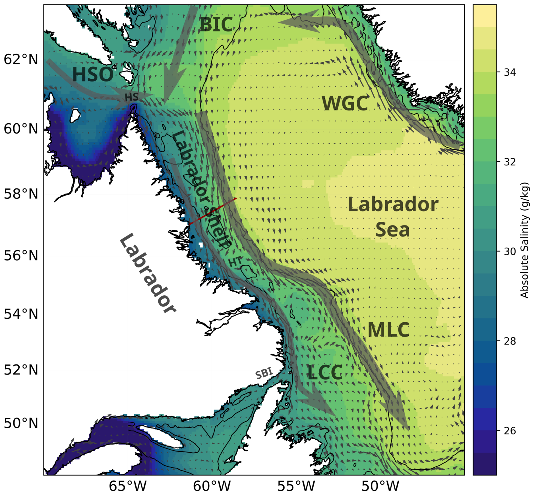
The Labrador Current System (LCS) forms part of the subpolar gyre circulation along the western boundary of the North Atlantic [1] (see Figure 1). The LCS consists of three branches: the Labrador Coastal Current (LCC), the main Labrador Current (MLC or LC), and the deep Labrador Current (DLC, below 1500 m; [2]). The currents all flow roughly along bathymetric contours in a generally south–southeasterly direction. The MLC lies over the upper continental slope along a strong salinity front that separates the fresher shelf waters (ca. 31.7–33.7 g/kg) from the more saline waters of the Labrador Sea (≳34.2 g/kg [2]; source values in practical salinity converted to absolute salinity using TEOS-10 [3]). The LCC lies entirely on the shelf and adjacent to the coast between the shelf waters and the even fresher coastal waters. Both of these currents have surface expressions with velocities that decrease with depth and lie along density fronts that contribute baroclinic components to their flow field. Source waters for the LCC and MLC include the Hudson Strait outflow, the Baffin Island Current, and the recirculating Atlantic waters of the Labrador Sea and western Greenland [4,5]. The DLC lies entirely at depth (below 1500 m) and is the Deep Western Boundary Current component of the Atlantic Meridional Overturning Circulation [6].
The LCC is the least studied branch of the LCS. Generally, there is an oceanographic data gap over the Labrador Shelf in regions closer to the coast, where the LCC lies. Existing data include the Atlantic Zone Monitoring Program (AZMP) which has established three CTD transects over the Labrador Shelf including stations in the near-coastal zone [7,8] and opportunistic sampling by research cruises that pass through the region (e.g., the Canadian Coast Guard Ship Amundsen [9]) and surface ocean drifters (e.g., the Global Drifter Program [5]). The AZMP lines off the Labrador coast include (from south to north) the Seal Island line (visited approximately annually) and the Makkovik Bank and Beachy Island lines which are visited more opportunistically when ship time and conditions allow (approximately once every 1–2 years and slightly less than once per 2 years, respectively [10]).
Figure 1. General surface circulation in the Labrador Sea and adjacent regions. The main circulation features on the Labrador Shelf include the main Labrador Current (MLC), located along the shelf edge, and the Labrador Coastal Current (LCC), located closer to the coast. Upstream circulation features that feed into the Labrador Shelf include the Hudson Strait Outflow (HSO), the Baffin Island Current (BIC), and the West Greenland Current (WGC). Regional features indicated include the Labrador Sea, the Labrador Shelf, Hudson Strait (HS), the Hopedale Trough (HT), and the Strait of Belle Isle (SBI). Also shown are the July–September climatological mean surface salinity (colors) and surface velocities (arrows) from the GLORYS reanalysis, bathymetric contours for depths of 150 m and 1500 m from GEBCO 2014 [11], and the Beachy Island AZMP line (red line).
Jmse 14 01163 g001
The LCC plays an important role in coastal ecosystems and sea ice dynamics. Sea ice along the northern Labrador Coast persists for up to 5–6 months of the year and is largely driven by local thermodynamic processes [12], indicating that the temperature and salinity of the coastal waters fed by the LCC in late Summer and Fall are key indicators for the following ice season. The coastal ice is of critical importance for Inuit communities in Nunatsiavut (Inuit self-governing region in northern Labrador) which rely on predictable, stable sea ice for fishing, hunting, and access to places of cultural importance [13] and a productive coastal ecosystem to support cultural practices and food security [14]. Geological records show evidence of links between the LCC, coastal ecosystems (e.g., productivity), and sea ice over the last 3000 years [15]. Coastal water properties fed by the LCC are also key factors in the distribution of geological features on the seafloor (e.g., subsea permafrost [16]). The dominant physical drivers of the LCC remain unclear and thus also unclear is the sensitivity of its transport and watermass properties to changes in local and upstream atmospheric, terrestrial and ocean conditions under anthropogenic climate change.
In this study we use a combination of surface ocean drifters and autonomous ocean gliders to characterize the LCS over the Labrador Shelf. We combine existing global drifter data [17] with additional surface drifters deployed off Labrador to fill in the near-coastal data gap. Both drifters and gliders have been recommended methods for observing ocean boundary current systems [18]. Surface drifters have been used successfully in the past to map circulation pathways in subpolar boundary currents [5,19,20]. Autonomous gliders have been used successfully to map hydrography across boundary currents and infer baroclinic and barotropic circulation components [21,22]. Here we will use these technologies to calculate surface tidal and non-tidal currents over the Labrador Shelf and current speeds and watermass properties of the LCC and MLC across the northern Labrador shelf.
This study is structured as follows. In Section 2, we present the surface drifter and glider data used here as well as processing methods to calculate tidal and non-tidal velocities from Lagrangian trajectories, to grid glider data, and to calculate velocities based on thermal wind shear. In the results (Section 3) we present tidal currents from drifters (Section 3.1), non-tidal currents from drifters (Section 3.2), velocities from gliders (Section 3.3), estimates of baroclinicity using the combined data (Section 3.4), and watermass properties of the LCC and MLC (Section 3.5). Finally, a summary and discussion is provided in Section 4.

2. Data and Methods

2.1. Ocean Drifters

Ocean drifters float on the ocean surface, drifting with ocean currents, and report their position at regular intervals. We use drifters from the Global Drifter Program (GDP) and the Community-Based Observations of Nunatsiavut Ocean Circulation (CONOC) project which consist of drifters of three types. Surface Velocity Program (SVP) drifters are the most common and consist of a spherical surface buoy attached to a nylon cylindrical drogue (a “holey sock”) that is tethered and weighted below the buoy to track ocean currents at 15-m depth [23]. The Coastal Dynamics Experiment (CODE), or Davis, drifter consists of a surface buoy rigidly attached to four sails, arranged in a cross-like shape, which project down over the top 1 m of the water to track surface currents [24]. Consortium for Advanced Research on Transport of Hydrocarbon in the Environment (CARTHE) drifters are similar in design to CODE drifters with the difference that the sails project down over the top 0.6 m of the water column and that the body is made from a biodegradable material [25].

2.1.1. Global Drifter Program

We obtained hourly, quality-controlled surface drifter data over the Labrador Shelf from the Global Drifter Program (GDP) [26]. We selected all drifters that passed within the rectangular domain (in latitude–longitude coordinates) bounded by 50° N, 61° N, 65° W and 50° W (see Figure 2a). From these drifters (n = 389) we obtained hourly positions (latitude, longitude), time, eastward velocity, and northward velocity. All GDP drifters were of the SVP type, and data spanned the 1995–2022 time period.

2.1.2. Community-Based Observations of Nunatsiavut Ocean Circulation

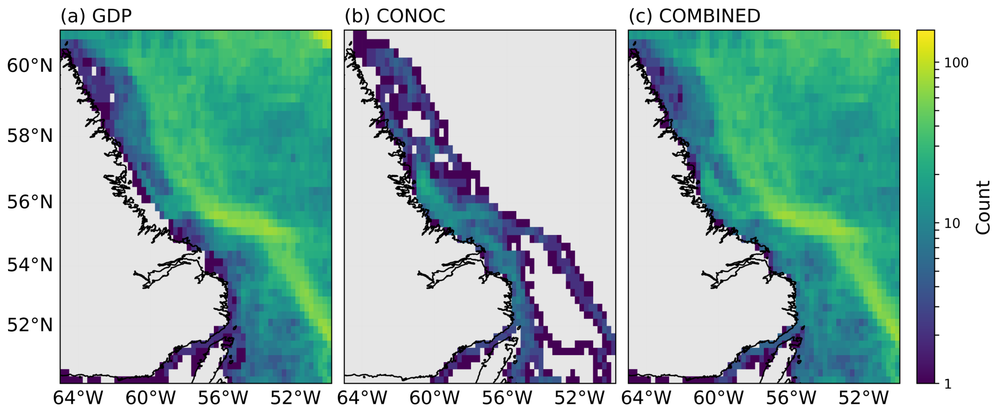
The Community-based Observations of Nunatsiavut Ocean Circulation (CONOC) project deployed CODE, SVP and CARTHE drifters off coastal Nunatsiavut (northern Labrador). The goal was to fill in the near-coast gap in the GDP data and do so with deployments based out of local communities. A total of 52 drifters were deployed from 2018 to 2022, and all fell within the Labrador Shelf bounding box defined above (Figure 2b). These drifters provide time and positional information on a range of sample rates (nominally 5 min for CARTHE drifters, 10 min for CODE drifters, and hourly for SVP drifters), and eastward and northward velocities were calculated from these positions using a first difference. The combined (GDP and CONOC) dataset reduces the data gap near the coast (Figure 2c).
The CONOC drifter data were quality-controlled as follows. Any clearly erroneous leading or trailing positions (e.g., pre-deployment positions recorded on land or en route, drifters that were picked up by fishing vessels, or run aground, etc.) were trimmed from the data. Occasionally, drifters displayed large jumps in position that returned to the previous location after a single time step indicating an erroneous GPS fix, and these positions were replaced with missing values. Given the near-coastal focus of the CONOC project, drifters were occasionally beached on land or were stuck on shoals, and data at these times were replaced with missing values. Occasional unrealistic lateral shifts in position were apparent, and these were treated by replacing the resulting large velocities by missing values. The resulting data were then bin-averaged into hourly position and velocity time series.
In this study, we combine the CONOC drifter data (2018–2022) and the GDP drifter data (1995–2022) into a single data set. We used GDP data for the entire time period rather than restricting it to the overlap with the CONOC data or the overlap with the glider data (2020–2021, presented below in Section 2.4) in order to have a large enough sample size to calculate mean current properties over a 1/4° degree grid. In doing so, we have assumed that the Labrador Current System, in terms of current speed and position, is largely stationary in time.

2.2. Tidal Decomposition

We assume that the drifter velocities u = ( u , v ) , where u and v are the eastward and northward components of velocity, can be decomposed into a sum of tidal u T and non-tidal u NT components:
u t = u t T + u t NT
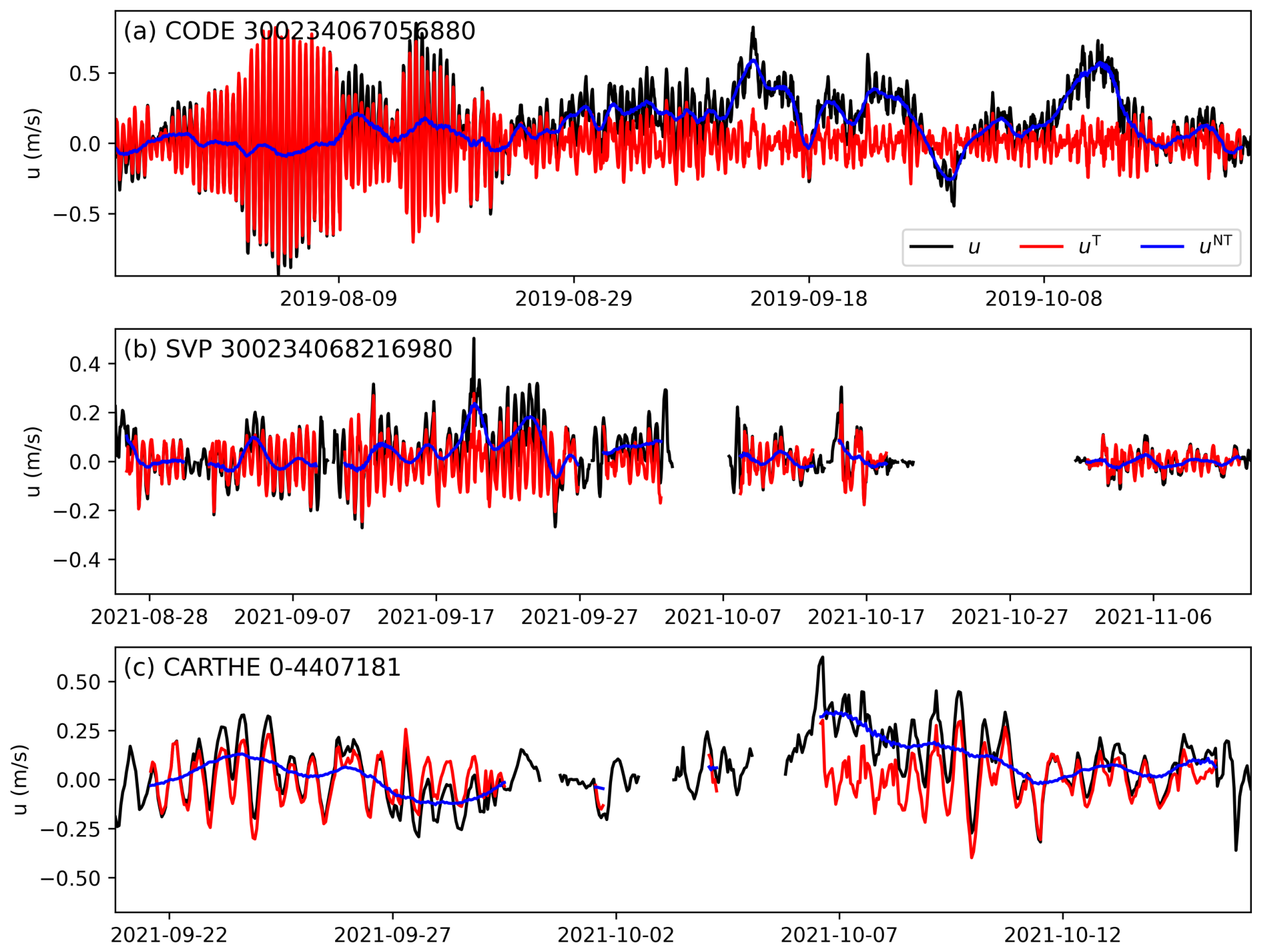
where t is the time index. For stationary time series, such as a mooring or tide gauge, the tidal component can be estimated by applying a tidal fit to the entire time series under the assumption that the amplitude of each tidal component does not vary in time. However, velocity time series from drifters are non-stationary since the drifters move spatially through different tidal regimes, which will be reflected in the velocity time series (Figure 3). Note that in Figure 3, the three drifter time series are shown over time periods of different lengths (less than 3 weeks to over 3 months) and so they show very different apparent tidal characteristics as the longer time series moves through more tidal regimes.
We use a moving window approach to do a non-stationary tidal decomposition. First, we define a window half-width as L h and the pool of L = 2 L h + 1 samples as
u t sample = { u s ; s = t L h , t L h + 1 , , t , , t + L h 1 , t + L h }
where L is the total window width. Since our drifter time series are hourly, L is in units of both hours and number of samples. We assume velocities are a linear combination of tidal (T) and non-tidal components (NT), i.e., u t = u t T + u t NT . We apply a tidal filtering operator F T to u t sample in order to remove the tidal component, i.e., u t NT = F T ( u t sample ) , and then determine the tidal component as u t T = u t u t NT . The tidal filter operator is one from a class of “tide killer” filters that are designed to preferentially damp oscillations on known tidal frequencies and therefore as distinct from tidal estimation using harmonic fits [27]. This operation is applied as a moving window over all values of t in u t except the first and last L h values, which are set to missing values. Before applying the tidal fit, we first interpolate linearly over missing value gaps of 3 h or less. We then use a window width of L = 39 h and a Doodson X0 “tide-killer” filter as the F T operator. The Doodson X0 filter is a 39-point weighted average filter designed to damp variability on the main tidal frequencies [28]. A demonstration of this tidal decomposition using both methods for three example drifters can be seen in Figure 3 (red and blue lines).

2.3. Gridding Process

The locations of the drifter velocities are not fixed, but move following the trajectories of the drifters. In order to generate a map of currents from the drifters we average the drifter velocity time series over fixed grid cells in space. We define a regular grid in longitude ( λ ) and latitude ( ϕ ) with a spacing of d λ = d ϕ (equal spacing in λ and ϕ ) such that { λ i = λ 0 + i d λ ; i = 1 , 2 N } and { ϕ j = ϕ 0 + j d ϕ ; j = 1 , 2 M } where N and M are the number of grid cells in the λ and ϕ directions respectively. The gridded currents at each ( i , j ) location, u i j , are thus defined as the average of all values of u t that fall within the grid cell defined by the intervals [ λ i , λ i + 1 ) and [ ϕ j , ϕ j + 1 ) . Note that this average is, in effect, both a spatial average over the footprint of this cell as well as a temporal average across all the times that drifters passed through this cell. The same method is applied to u t NT and u t T to generate maps of non-tidal currents u i j NT and mean tidal current speed u i j T , respectively. Note that for tidal currents, we only report the mean current speed, which is | u | = u 2 + v 2 . Here we have used d λ = d ϕ = 0.25 ° , λ 0 = 65 ° W and ϕ 0 = 50 ° N with the resulting { λ i } and { ϕ j } spanning the rectangular domain used above (Figure 2). The total sample counts contributing to each grid cell average can be seen in Figure 4.

2.4. Gliders

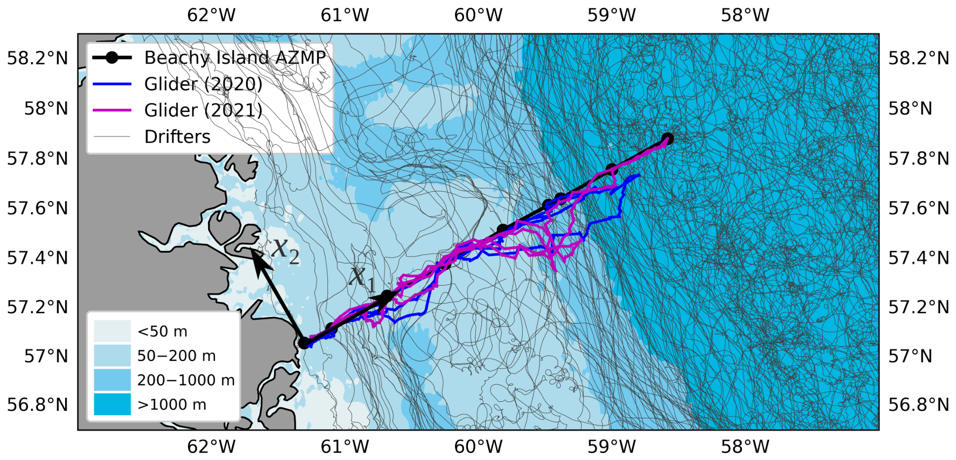
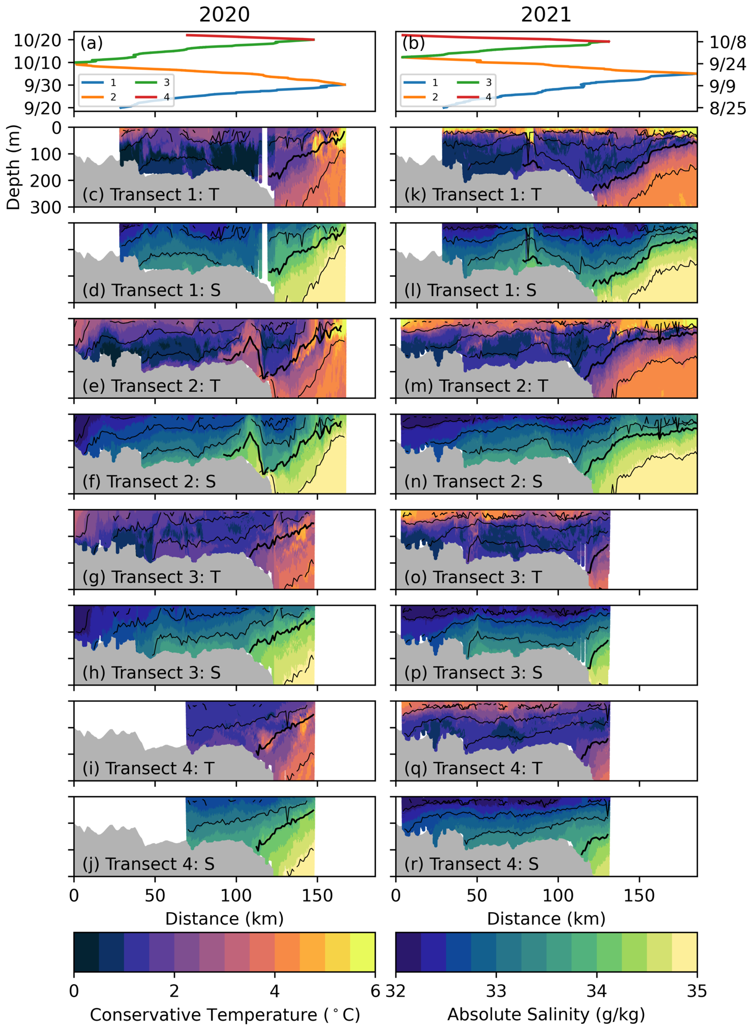
The Beachy Island AZMP line runs perpendicular to the Labrador Shelf and intersects the coast around 57° N (Figure 1, red line; Figure 5, black line and dots). A Slocum glider was deployed along this line in 2020 and again in 2021 (Figure 5, blue and magenta lines). There were two missions, one in 2020 (lasting 34 days, from 20 September 2020 to 23 October 2020) and one in 2021 (lasting 50 days, from 25 August 2021 to 13 October 2021). Glider locations with time indicate multiple, repeat transects (Figure 6a,b). The gliders were equipped with a Seabird GPCTD which was set to sample at 1 Hz. The vertical velocity of the gliders was predominantly between 21 and 34 cm/s which means there were approximately 3 to 4 data points per meter. There were occasional instances when the gliders’ speed was increased by the pilots to help fight currents. In these situations the gliders’ vertical velocity increased to a range between 38 and 46 cm/s which led to approximately 2 data points collected per meter.
Although the glider collected data on several variables including chlorophyll-a, fluorescence, oxygen concentration, optical backscattering and downwelling irradiance, in this study only the following data were used: latitude ϕ , longitude λ , pressure p, depth d, temperature T, practical salinity S and density ρ . From these variables we derived absolute salinity S A , conservative temperature Θ , and potential density anomaly (relative to 0 dbar) σ using TEOS-10 and the Gibbs-SeaWater oceanographic toolbox [3] (Figure 6c–r). These data were obtained from https://erddap.oceantrack.org/erddap/tabledap/index.html (accessed on 3 March 2025) using Dataset ID’s otn200_20200920_118_delayed and otn200_20210825_139_delayed.
Note that the glider includes a flight model that predicts the location of each surfacing based on the given flight parameters, under the assumption of no background current flow. The difference between the actual surfacing position and the expected position can be used to estimate depth-mean currents. However, in these missions, an on-board thruster was used at times to control the flight, since we expected the large current speeds in the Labrador current to push the glider far off its planned trajectory. As a consequence we cannot use the flight model and actual positions to estimate depth mean current speeds.
Seawater density data from the 2020 and 2021 glider transects were combined into a single dataset. Both glider tracks followed approximately the Beachy Island AZMP line and so we gridded the glider data on an ( x 1 , z) grid oriented along this line (Figure 5, black axes). We used a bi-linear interpolation onto a regular grid with x 1 having spacing every 1.9 km, and z using the GLORYS vertical coordinate system. Any extrapolated data below the deepest depth reached by the gliders (typically ∼350 m), at each x 1 , was removed to obtain ρ ( x 1 , z ) . We then smoothed the gridded density field in the x 1 direction using a 5-point (ca. 9.4 km) equal-weighted running window to obtain ρ sm ( x 1 , z ) .
Geostrophic velocities were estimated using the thermal wind relationship
f u 2 z = g ρ 0 ρ sm x 1
where u 2 is the velocity in the x 2 direction, g = 9.8 m/s is gravitational acceleration, ρ 0 = 1024 kg/m3 is the background density, and f = 1.23 × 10 4 s−1 is the Coriolis parameter (assumed to be constant across the small range of latitudes sampled by the gliders). By vertically integrating this equation, we can write
u BC ( z ) = u 2 ( z ) u 2 ( H ) = g f ρ 0 H z ρ sm x 1 d z
where u 2 ( z ) is the velocity at some vertical level z, and when referenced to the velocity at the bottom ( z = H ), we take this to represent u BC , the baroclinic component of the flow. This is the geostrophic current velocity at depth z referenced to the bottom geostrophic current velocity. We assume that the barotropic component of the flow u BT is uniform in the vertical, and that the total flow u ( z ) is given by the sum of the two components: u ( z ) = u BC ( z ) + u BT . At the surface ( z = 0 ) , the total flow u ( 0 ) may be estimated from our surface drifters. So, in this study, we can do a decomposition of the surface flow into barotropic and baroclinic components but we have no way to do this for the interior since we lack an estimate of u ( z ) in the ocean interior. Note that in this decomposition we have ignored any vertically sheared flow that may arise due to balances other than by thermal wind (e.g., wind-driven Ekman flow).

2.5. Transports

Given velocities perpendicular to the Beachy Island line and the glider transect u 2 ( x 1 , z ) , conservative temperature Θ ( x 1 , z ) and absolute salinity S A ( x 1 , z ) , we can calculate volume, heat and freshwater transports. Volume transport across the section is given by
T V = x c x o H 0 u 2 d z d x
in m3/s, which we express here in Sv (=106 m3/s), where the integral has been evaluated between a coastal location x c and offshore location x o in the cross-shelf ( x 2 ) direction. Heat transport is given by
T Q = x c x o H 0 Q u 2 d z d x
in W, which we express here in PW (=1015 W), and where Q ( x 1 , z ) = Θ c p ρ is the ocean heat content, c p = 3992 J K−1 kg−1 is the specific heat capacity of seawater [3], and ρ is seawater density. Freshwater transport is given by
T F = x c x o H 0 F u 2 d z d x
in m3/s, which we express here in mSv (=10−3 m3/s), and where F ( x 1 , z ) = 1 S A / S 0 is the freshwater content and S 0 is a reference salinity [29]. Typical practical salinity values used for S 0 in subarctic North Atlantic studies are 34.8 [4] or 35.0 [1]. In this study we use corresponding absolute salinity values of 34.95 g/kg or 35.15 g/kg, respectively.

2.6. GLORYS Reanalysis

Daily fields of temperature, salinity and eastward and northward velocity were obtained from the GLORYS12V1 reanalysis on a 1/12° grid in latitude and longitude [30]. Density was derived from temperature and salinity using TEOS-10 and the Gibbs-SeaWater oceanographic toolbox [3]. The vertical resolution consists of 50 z-levels unevenly spaced with higher resolution (1–5 m) near the surface. Data were obtained covering the 1993–2019 period. Annual mean climatologies were created for all variables by averaging data across all time for each latitude, longitude and depth. Geostrophic velocities associated with the GLORYS density field are estimated in the same way as described above for the glider data; the GLORYS density field is not further smoothed.

3. Results

We first present the spatial distribution of tidal current speeds (Section 3.1) and mean non-tidal current velocities (Section 3.2) for the combined drifter datasets. We then examine the cross-shelf structure of the LCC and MLC as represented in the drifter and glider datasets including velocity structure (Section 3.3), baroclinicity (Section 3.4) and watermass properties (Section 3.5).

3.1. Tidal Currents

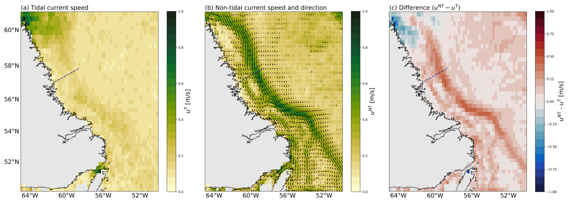
Tidal current speeds are generally weak (<0.3 m/s) over most of the Labrador Shelf and even weaker (<0.1 m/s) over waters deeper than the shelf (Figure 7a). There are two areas where tidal currents are stronger. First, over the shelf off the northernmost part of Labrador (north of 58.5° N) and into the Hudson Strait, tidal currents are generally >0.4 m/s and up to 1.0 m/s. Second, in the Strait of Belle Isle between Labrador and Newfoundland, tidal currents are similarly large.

3.2. Mean Currents

Non-tidal current velocities reproduce the circulation associated with the Labrador Current System (Figure 7b). The strongest currents (0.5–0.9 m/s) are found in a contiguous band along the shelf edge directed in a southeasterly direction, associated with the MLC. This current appears to be contiguous with the strong (∼0.5 m/s) outflow from the Hudson Strait off the northern tip of Labrador.
There is a discontinuous band of moderate current speeds (up to 0.5 m/s) closer to the Labrador coast, directed along-shore in a generally southeasterly direction, associated with the LCC. From north to south we find the following regimes. From the northern tip of Labrador, the LCC appears along the coast south as far as ∼59.40° N after which the currents near the coast and over the shelf are generally very weak. Over 57.20–58.30° N there is some exchange from the MLC to the LCC. The LCC is then quite coherent and distinct from the MLC over the 55.32–58.15° N latitudinal range. Over the Hopedale Trough (55.30–56.25° N) there is topographically steered flow leading to exchange from the MLC towards the coastal current followed by exchange from the LCC towards the MLC. South of 54.9° N, the LCC regains coherency and remains so as far as Belle Isle at which point it bifurcates into a flow that passes through the Strait of Belle Isle (and along the lower north shore of the Gulf of St. Lawrence) and a flow that follows the northeast coastline of Newfoundland.

3.3. Cross-Shelf Transects

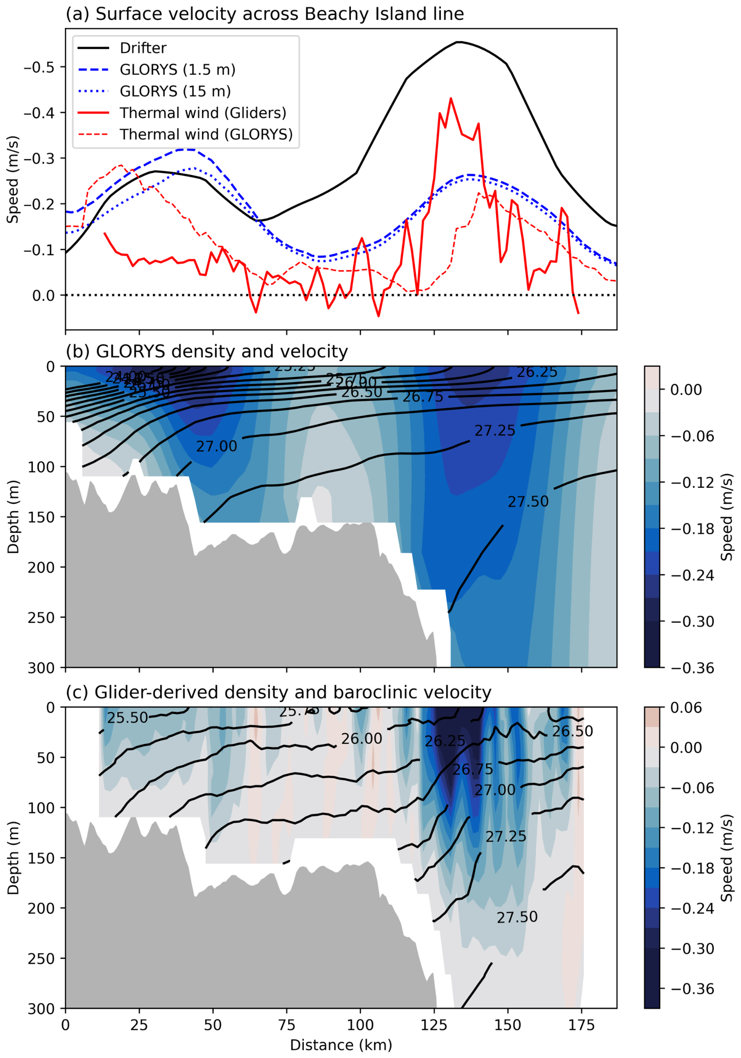
The along-shelf velocities from the gridded drifter data at the location of the Beachy Island transect line clearly show two distinct jets (Figure 8a, black line). The LCC peaks around 25–50 km from the coast, in approximately 100 m water depths, at nearly 0.3 m/s, and the MLC peaks around 125–150 km from the coast (at the edge of the shelf) at over 0.5 m/s. All along the transect we see southward flows across the transect. The reanalysis velocities from climatological July–September GLORYS indicate the same structure with current locations at similar distances from the coast, but with weaker peak speeds (0.2 m/s for the LCC, 0.3 m/s for the MLC; Figure 8a, blue lines). Note that GLORYS data are shown for both the 1.5 m and 15 m depths as proxies for the depths sampled by the different drifter types (ca. 1 m for CODE and CARTHE drifters, 15 m for SVP drifters); the mean currents from GLORYS at these two depths are very similar (a root mean squared error of <0.03 m/s) indicating that we can expect small errors due to combining the three different drifter types.
The vertical structure of the current system from GLORYS indicates velocities of the same sign all throughout the water column, and increasing in magnitude closer to the surface (Figure 8b, blue shading) consistent with baroclinic flows driven by thermal wind shear associated with the across-shelf density gradient. The climatological July–September GLORYS density field indicates isopycnals that universally slope upwards with distance away from the coast, at all depths (Figure 8b, black contours). The strongest slopes are seen near where the two current jets appear (see above). The surface geostrophic flows (referenced to the bottom; Figure 8a, red line) are broadly consistent with the total velocities taken directly from GLORYS.
The density field from the glider data (Figure 8c, black contours) is broadly consistent with the density field from GLORYS. It differs most significantly in that there is a very strong density gradient within 5–10 km of the coast due to low salinity, near-surface waters that do not appear in GLORYS. The geostrophic surface velocities associated with this density field indicate an MLC with velocities up to 0.35 m/s and an LCC with speeds 0.1–0.2 m/s in the same location as in the other data set but increasing as high as 0.35 m/s very close to the coast due to the strong density (salinity) gradients there.

3.4. Barotropic and Baroclinic Components

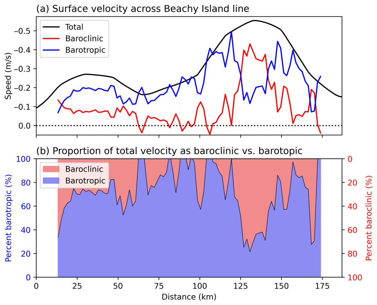
We can combine the drifter and glider data to estimate the barotropic component of the velocity in the LCC and MLC. We take the thermal wind velocities, referenced to the bottom, to represent the baroclinic component of the surface velocities (Figure 9a, red line; Figure 8a, red line). Assuming the total velocity at the surface is represented by the surface drifters (Figure 9a, black line; Figure 8a, black line), that the total is simple a linear combination of the baroclinic and barotropic components, and that the barotropic component is uniform in the vertical, then we can estimate the barotropic component by subtracting the baroclinic component at the surface from the total at the surface (Figure 9a, blue line). The barotropic component of the flow across the Beachy Island line is generally >0.1 m/s everywhere and does not exhibit a strong distinction between the LCC and the (baroclinically) quiescent flows of the mid-shelf region between the LCC and the LC. The barotropic component of the MLC is larger (0.2–0.4 m/s). The surface LCC velocities are predominantly barotropic (ca. 70%; Figure 9, blue shading), the mid–shelf velocities are dominated by the barotropic component (ca. 70–80+%; Figure 9, blue shading), and the main LC is predominantly baroclinic in nature (ca. 70%; Figure 9, red shading).

3.5. Watermass Properties and Transports

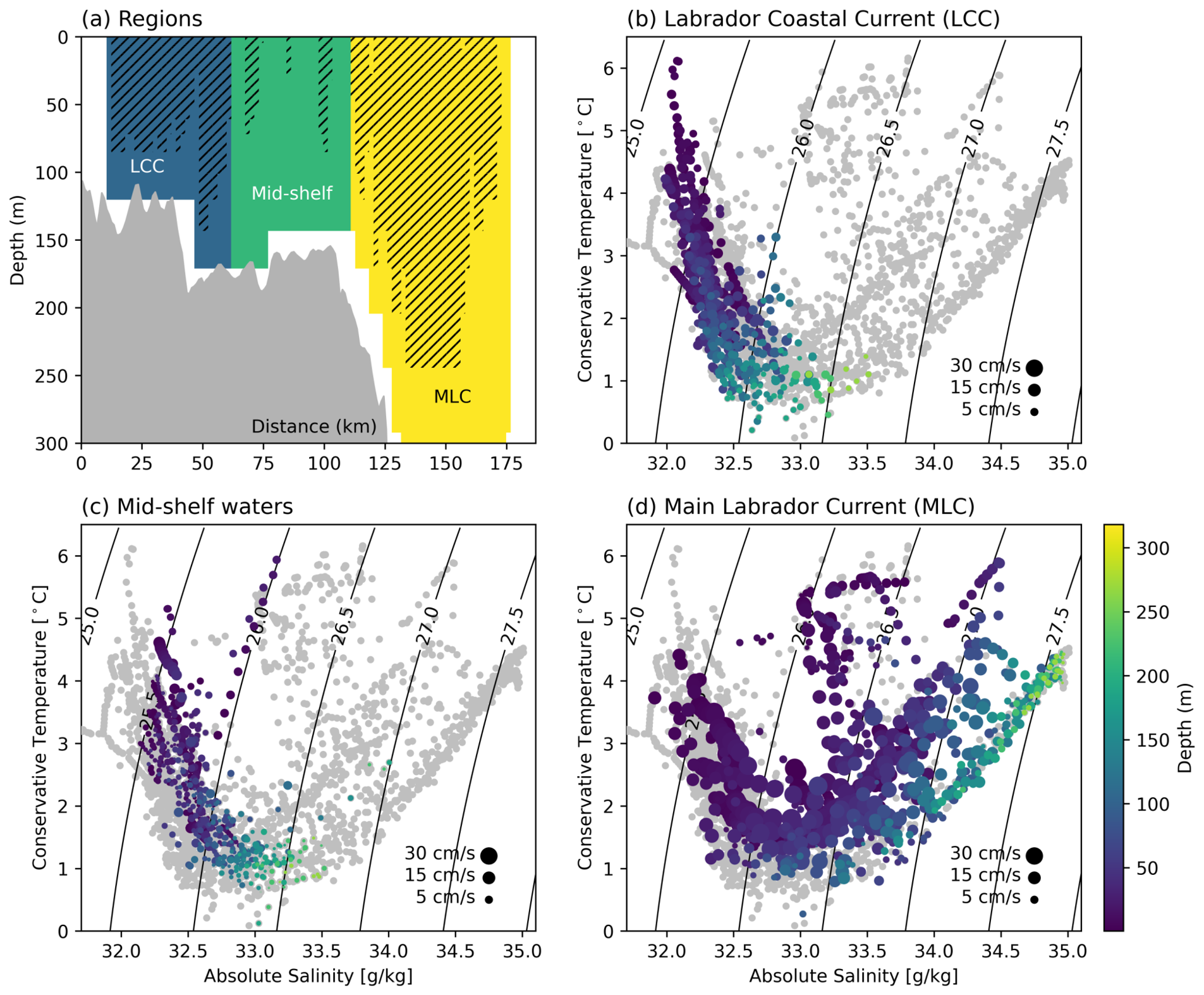
The watermass properties of the LCS over the shelf exhibit distinctions amongst the different branches of the flow (Figure 10). We define three regions in the x 1 -z plane along the Beachy Island line from the glider data (Figure 10a) as follows. The LCC region covers the first 63 km from the coast, the mid-shelf region covers from 63 km to 110 km, and the MLC region covers from 110 km to the end of the transect (Figure 10a, colored areas). We can see that there is a contiguous block of southward baroclinic velocities in each of the LCC and MLC regions, while the mid-shelf region includes several smaller disconnected areas of southward flow (Figure 10a, hatched areas show u BC < 0.03 m/s). The waters of the LCC are almost entirely fresher than 33 g/kg with most values centered around 32.5 g/kg (Figure 10b). The T-S relationship for the LCC is such that warmer waters are also less saline and occur at shallower depths. The mid-shelf waters occupy a salinity range slightly higher than the LCC (32.25–33.5 g/kg) with a similar T-S-depth relationship (Figure 10c). The MLC occupies a very broad range of salinity values (32–35 g/kg) with the core of the jet occupying the middle of this range (Figure 10d). For shallow depths (<50 m) the T-S-depth relationship is similar to the LCC; for deeper depths, we find that both temperature and salinity increase together with depth. Quiescent coastal waters and quiescent offshore waters (not shown) tend to occupy the edges of the LCC and MLC spaces described above.
Volume, heat and freshwater transports were calculated for each of the LCC, mid-shelf, and MLC regions (Table 1) using temperature, salinity and velocities across our transect following the methods outlined in Section 2.5. The LCC has a volume transport of 1.34 Sv, about 20% of which is due to the baroclinic component of the flow, while the mid-shelf has a similar volume transport of 1.63 Sv, nearly all of which is due to the barotropic component of the flow (i.e., the baroclinic flow is nearly absent over the mid-shelf, as seen earlier in Figure 9). The MLC has a much larger volume transport of 6.51 Sv. Note that these transports are only calculated down to 300 m (the maximum depth of the glider paths) and the MLC reaches much deeper, meaning the total volume transport over all depths is larger than this number. Heat transports show a similar pattern with 1.51 PW in the LCC, 1.83 PW across the mid-shelf, and 7.38 PW in the MLC.
Freshwater transports show that the LCC transports about half the freshwater compared to the MLC (89.0 mSv for the LCC, 166 mSv for the MLC). Freshwater transport over the mid-shelf (91.8 mSv) is similar to the LCC and when taken together the LCC and mid-shelf have a larger combined freshwater transport than the MLC. This is despite much weaker volume transport and is due to the lower salinity coastal and mid-shelf waters. These freshwater transports were calculated using a reference salinity of 34.95 g/kg (practical salinity of 34.8). Slightly larger numbers, though showing the same pattern across the shelf, are found using a reference salinity of 35.15 g/kg (practical salinity of 35.0; see Table 1).

4. Summary and Discussion

In this study, we characterize the Labrador Coastal Current (LCC) in terms of current speed, cross-shelf structure, baroclinicity, volume and freshwater transports and watermass properties. This is done by combining two independent observational datasets, surface drifter derived velocities and autonomous glider-derived temperature and salinity profiles, and comparing these results with estimates from a global ocean reanalysis. Drifter velocities are decomposed into tidal and non-tidal components and gridded. Gliders profiles are assembled into transects along the Beachy Island AZMP line and used to calculate thermal wind shear in the along-shelf direction. The baroclinic component of the flow is assumed to be represented by the thermal wind shear, referenced to the bottom, and the total (baroclinic plus barotropic) flow is assumed to be represented by the surface drifter-derived velocity, from which we can infer the barotropic component of the flow.
Surface tidal currents are generally weak over the Labrador Shelf, and weaker than the mean non-tidal currents, except in the Hudson Strait, the adjacent northern portion of the shelf, and in the Strait of Belle Isle. Mean surface non-tidal currents exhibit a clear Hudson Strait Outflow, a two-branch Labrador Current System (LCC and Main Labrador Current, MLC), some indication of flow along isobaths in both branches including potential exchange between the branches, and flow through the Strait of Belle Isle. Along the Beachy Island AZMP line, the LCC lies over the inner portion of the shelf, approximately over water depths of 100–150 m, with maximum surface speeds of ca. 0.25 m/s, while the MLC lies over the continental slope with maximum surface speeds of ca. 0.5 m/s. This pattern is broadly consistent between the drifter-derived velocities, the glider-derived thermal wind shear, and the global ocean reanalysis—although the glider data shows the LCC to be broader and weaker over the inner half of the shelf. The LCC is dominated (70%) by the barotropic component of the flow while the MLC is dominated (70%) by the baroclinic component of the flow. The LCC includes the freshest watermasses over the shelf, with salinity always fresher than 33 g/kg, while the MLC includes water with salinity in the 32–35 g/kg range. The volume transport, in the upper 300 m, is over four times greater in the MLC (6.51 Sv) than in the LCC (1.34 Sv, or 2.97 Sv if the mid-shelf is included). In contrast, the freshwater transport in the LCC (89 mSv) is over half that of the MLC (166 mSv) and the combined freshwater transport of the LCC and mid-shelf (181 mSv) is greater than the MLC.
We have taken a multi-platform approach to characterizing the Labrador Current System. By supplementing the Global Drifter Program data with drifter data from the CONOC project, this study has filled in a notable data gap along the coastal portion of the Labrador Shelf. We have further complemented these surface data with subsurface hydrographic measurements from the first glider missions in the region. We draw on the strengths of each source of data, the gliders being most useful at providing estimates of thermal wind and the drifters most useful at providing estimates of total absolute surface velocities, to undertake a combined analysis that synthesizes across the datasets. In doing so, we could estimate both the baroclinic and barotropic components of the LCC and MLC, watermass properties, volume, heat and freshwater transports.
The limitations of this study are as follows. First, the surface drifter velocities we take to be a combination of a vertically uniform barotropic component and the vertically sheared baroclinic component (from thermal wind). However, surface winds will contribute a vertically sheared Ekman flow captured by the surface drifters that we have not accounted for. This could be done, but would require estimates of the time- and space-varying wind field and a model for the non-steady Ekman response of the surface ocean. Second, we have estimated heat transports using temperature and velocities across our transects. However, absolute heat transports across a partial section (i.e., our transect runs from the coast to the open ocean) are less useful than one that spans a basin from coast to coast (e.g., the AR7W line). The latter can be used to estimate the net heat that is exchanged between basins while the former is largely reflecting volume transports in boundary currents alone. Third, we have used drifters spanning several months (centered on July) across 5 years and gliders spanning three months across two years (centered on August) together in a synthesized, multi-platform analysis. The drifter and glider data are not perfectly coincident in time and thus there may be uncertainties that arise due to this temporal mismatch. Finally, while we have estimated tidal current speed amplitudes, we have not performed a tidal component analysis and thus the utility of our results for validating tidal model output remains incomplete.
This study effectively provides a data set that can be used for model validation, for understanding circulation, and for informing future hypotheses. The maps of tidal and non-tidal current speeds will be valuable for validating numerical ocean circulation models in the region. Studies on North Atlantic subpolar gyre and Atlantic meridional overturning circulation rely on estimates of volume, heat and freshwater transports in the various branches and boundary currents and here we provide new values, independent of previous studies, which can be added to the existing sources. Finally, our results will inform future studies by generating hypotheses for testing. For example, if the LCC is predominantly barotropic in nature, it may not be very sensitive to variations in Arctic runoff; identifying the role of the strong tidal currents in the northern Labrador shelf in vertical mixing and ice-ocean heat flux; and understanding the degree to which bathymetric steering of the LCC and MLC contribute to cross-shelf exchange of heat, freshwater, and other tracers.

Author Contributions

Conceptualization, E.C.J.O. and C.R.; methodology, E.C.J.O. and C.R.; software, E.C.J.O.; formal analysis, E.C.J.O.; investigation, E.C.J.O. and C.R.; resources, E.C.J.O.; data curation, E.C.J.O.; writing—original draft preparation, E.C.J.O. and C.R.; writing—review and editing, E.C.J.O. and C.R.; visualization, E.C.J.O.; project administration, E.C.J.O.; funding acquisition, E.C.J.O. and C.R. All authors have read and agreed to the published version of the manuscript.

Funding

This research was funded by Crown-Indigenous Relations and Northern Affairs Canada (CIRNAC) grant number CBM-NUT-050-2018 (“Community-based Observations of Nunatsiavut Ocean Circulation”) and National Sciences and Engineering Research Council of Canada (NSERC) Discovery Grant number RGPIN-2018-05255 (“Prediction and predictability of climate extremes”).

Institutional Review Board Statement

The study was approved by the Nunatsiavut Government Research Advisory Committee (29 May 2018).

Data Availability Statement

The glider data is publicly available on the Ocean Tracking Network ERDDAP server at https://erddap.oceantrack.org/erddap/tabledap/index.html (accessed on 15 June 2026).

Acknowledgments

The Dalhousie glider was prepared by the Coastal Environmental Observation Technology and Research (CEOTR) group (ceotr.ocean.dal.ca). Support for the deployment and operation of this mission was provided by the Nunatsiavut Government (NG), Oceans North, the Ocean Tracking Network, and the MV What’s Happening. Data were collected in a region governed by the Nunatsiavut Government (NG), and the data belong to NG. Specific acknowledgements for their role in drifter and glider deployments and data processing: Joey Angnatok, Sid Pain, Adam Comeau, Tyler Byrne, Fernando Sobral, Liz Pijogge, John Winters, Taylor Davies. Special acknowledgements to the late Keith Thompson for prompting the initial idea that grew into the CONOC project. We would like to acknowledge Frederic Cyr for providing the coordinates of the Beachy Island AZMP sites. The GLORYS12V1 data product (doi: 10.48670/moi-00021) was obtained from the Copernicus Marine Service Information (CMEMS) system.

Conflicts of Interest

The authors declare no conflicts of interest. The funders had no role in the design of the study; in the collection, analyses, or interpretation of data; in the writing of the manuscript; or in the decision to publish the results.

References

  1. Loder, J.; Petrie, B.; Gawarkiewicz, G. The coastal ocean off northeastern North America: A large-scale view. Sea 1998, 11, 105–133. [Google Scholar]
  2. Lazier, J.R.; Wright, D.G. Annual velocity variations in the Labrador Current. J. Phys. Oceanogr. 1993, 23, 659–678. [Google Scholar] [CrossRef][Green Version]
  3. McDougall, T.J.; Barker, P.M. Getting Started with TEOS-10 and the Gibbs SEAWATER (GSW) Oceanographic Toolbox; SCOR/IAPSO WG 127: Berlin, Germany, 2011; 28p. [Google Scholar]
  4. Florindo-López, C.; Bacon, S.; Aksenov, Y.; Chafik, L.; Colbourne, E.; Holliday, N.P. Arctic Ocean and Hudson Bay freshwater exports: New estimates from seven decades of hydrographic surveys on the Labrador Shelf. J. Clim. 2020, 33, 8849–8868. [Google Scholar] [CrossRef]
  5. Duyck, E.; Foukal, N.P.; Frajka-Williams, E. Circulation of Baffin Bay and Hudson Bay waters on the Labrador shelf and into the subpolar North Atlantic. Ocean. Sci. 2025, 21, 241–260. [Google Scholar] [CrossRef]
  6. Handmann, P.; Fischer, J.; Visbeck, M.; Karstensen, J.; Biastoch, A.; Böning, C.; Patara, L. The deep western boundary current in the Labrador Sea from observations and a high-resolution model. J. Geophys. Res. Ocean. 2018, 123, 2829–2850. [Google Scholar] [CrossRef]
  7. Therriault, J.C. Proposal for a Northwest Atlantic Zonal Monitoring Program; Canadian Technical Report of Hydrography and Ocean Sciences; Fisheries and Oceans Canada: Ottawa, ON, Canada, 1998; 57p. [Google Scholar]
  8. Pépin, P.; Petrie, B.; Therriault, J.; Narayanan, S.; Harrisson, W.; Frank, K.; Chassé, J.; Colbourne, E.; Gilbert, D.; Gregory, D.; et al. The Atlantic Zone Monitoring Program (AZMP): Review of 1998–2003; Canadian Technical Report of Hydrography and Ocean Sciences; Fisheries and Oceans Canada: Ottawa, ON, Canada, 2005; 87p. [Google Scholar]
  9. Ratsimbazafy, T.; Dezutter, T.; Desmarais, A.; Amirault, D.; Guillot, P.; Morisset, S. Oceanographic dataset collected during the 2021 scientific expedition of the Canadian Coast Guard Ship Amundsen. Earth Syst. Sci. Data Discuss. 2023, 16, 471–499. [Google Scholar]
  10. Coyne, J.; Cyr, F.; Donnet, S.; Galbraith, P.; Geoffroy, M.; Hebert, D.; Layton, C.; Ratsimandresy, A.; Snook, S.; Soontiens, N.; et al. Canadian Atlantic Shelf Temperature-Salinity (CASTS); Federated Research Data Repository: Waterloo, ON, Canada, 2023. [Google Scholar]
  11. GEBCO Bathymetric Compilation Group. The GEBCO_2026 Grid—A Continuous Terrain Model for Oceans and Land at 15 Arc-Second Intervals. Available online: https://www.bodc.ac.uk/data/published_data_library/catalogue/10.5285/4f68d5c7-45eb-f999-e063-7086abc036fa (accessed on 15 June 2026).
  12. Codiga, D.L. Unified Tidal Analysis and Prediction Using the UTide Matlab Functions; Technical Report 2011-01; Graduate School of Oceanography, University of Rhode Island: Narragansett, RI, USA, 2011. [Google Scholar]
  13. Brice-Bennett, C. Our Footprints Are Everywhere: Inuit Land Use and Occupancy in Labrador; Labrador Inuit Association: Nain, NL, Canada, 1977. [Google Scholar]
  14. Miatta, M.; Snelgrove, P.V.; Bates, A.E.; Bailey, M.; Bradbury, I.R.; Cadman, R.; Campanyà-Llovet, N.; Clinton, M.E.; Cote, D.; Denniston, M.; et al. Developing socio-ecological indicators for changing Northern Coastal environments. Facets 2025, 10, 1–18. [Google Scholar] [CrossRef]
  15. Atkinson, M.; Normandeau, A.; Van Nieuwenhove, N.; de Vernal, A.; Saunders, M.; Woollett, J.; Limoges, A. Labrador Coastal Current and productivity variations offshore Nain (Nunatsiavut) during the late Holocene. Quat. Sci. Rev. 2024, 337, 108790. [Google Scholar] [CrossRef]
  16. Normandeau, A.; Eamer, J.B.; Way, R.G.; Harrison, E.J.; Cyr, F.; Algar, C.K.; Eamer, J.L.; Geizer, H.D.; Haddock, J.; Kurylyk, B.L.; et al. Evidence for subsea permafrost in subarctic Canada linked to submarine groundwater discharge. Nat. Geosci. 2024, 17, 1022–1030. [Google Scholar] [CrossRef]
  17. Lumpkin, R.; Johnson, G.C. Global ocean surface velocities from drifters: Mean, variance, El Niño–Southern Oscillation response, and seasonal cycle. J. Geophys. Res. Ocean. 2013, 118, 2992–3006. [Google Scholar] [CrossRef]
  18. Todd, R.E.; Chavez, F.P.; Clayton, S.; Cravatte, S.; Goes, M.; Graco, M.; Lin, X.; Sprintall, J.; Zilberman, N.V.; Archer, M.; et al. Global perspectives on observing ocean boundary current systems. Front. Mar. Sci. 2019, 6, 423. [Google Scholar] [CrossRef]
  19. Cuny, J.; Rhines, P.B.; Niiler, P.P.; Bacon, S. Labrador Sea boundary currents and the fate of the Irminger Sea Water. J. Phys. Oceanogr. 2002, 32, 627–647. [Google Scholar] [CrossRef]
  20. Duyck, E.; De Jong, M.F. Circulation over the South-East Greenland Shelf and potential for liquid freshwater export: A drifter study. Geophys. Res. Lett. 2021, 48, e2020JB020886. [Google Scholar] [CrossRef]
  21. Dever, M.; Hebert, D.; Greenan, B.; Sheng, J.; Smith, P. Hydrography and coastal circulation along the Halifax Line and the connections with the Gulf of St. Lawrence. Atmos.-Ocean 2016, 54, 199–217. [Google Scholar] [CrossRef]
  22. Dever, M.; Skagseth, Ø.; Drinkwater, K.; Hebert, D. Frontal Dynamics of a Buoyancy-Driven Coastal Current: Quantifying Buoyancy, Wind, and Isopycnal Tilting Influence on the Nova Scotia Current. J. Geophys. Res. Ocean 2018, 123, 4988–5003. [Google Scholar] [CrossRef]
  23. Lumpkin, R.; Pazos, M. Measuring surface currents with Surface Velocity Program drifters: The instrument, its data, and some recent results. Lagrangian Anal. Predict. Coast. Ocean Dyn. 2007, 39, 67. [Google Scholar]
  24. Davis, R.E. Drifter observations of coastal surface currents during CODE: The method and descriptive view. J. Geophys. Res. Ocean 1985, 90, 4741–4755. [Google Scholar] [CrossRef]
  25. Novelli, G.; Guigand, C.M.; Cousin, C.; Ryan, E.H.; Laxague, N.J.; Dai, H.; Haus, B.K.; Özgökmen, T.M. A biodegradable surface drifter for ocean sampling on a massive scale. J. Atmos. Ocean. Technol. 2017, 34, 2509–2532. [Google Scholar] [CrossRef]
  26. Elipot, S.; Sykulski, A.; Lumpkin, R.; Centurioni, L.; Pazos, M. Hourly Location, Current Velocity, and Temperature Collected from Global Drifter Program Drifters World-Wide; Version v2.01; NOAA National Centers for Environmental Information: Asheville, NC, USA, 2022. [Google Scholar] [CrossRef]
  27. Thompson, R. Low-pass filters to suppress inertial and tidal frequencies. J. Phys. Oceanogr. 1983, 13, 1077–1083. [Google Scholar] [CrossRef]
  28. Doodson, A.T. VI. The Analysis of Tidal Observations. In Philosophical Transactions of the Royal Society of London; Series A—Containing Papers of a Mathematical or Physical Character; Taylor and Francis: London, UK, 1928; Volume 227, pp. 223–279. [Google Scholar]
  29. Schauer, U.; Losch, M. “Freshwater” in the ocean is not a useful parameter in climate research. J. Phys. Oceanogr. 2019, 49, 2309–2321. [Google Scholar] [CrossRef]
  30. Jean-Michel, L.; Eric, G.; Romain, B.B.; Gilles, G.; Angélique, M.; Marie, D.; Clément, B.; Mathieu, H.; Olivier, L.G.; Charly, R.; et al. The copernicus global 1/12 oceanic and sea ice GLORYS12 reanalysis. Front. Earth Sci. 2021, 9, 698876. [Google Scholar] [CrossRef]
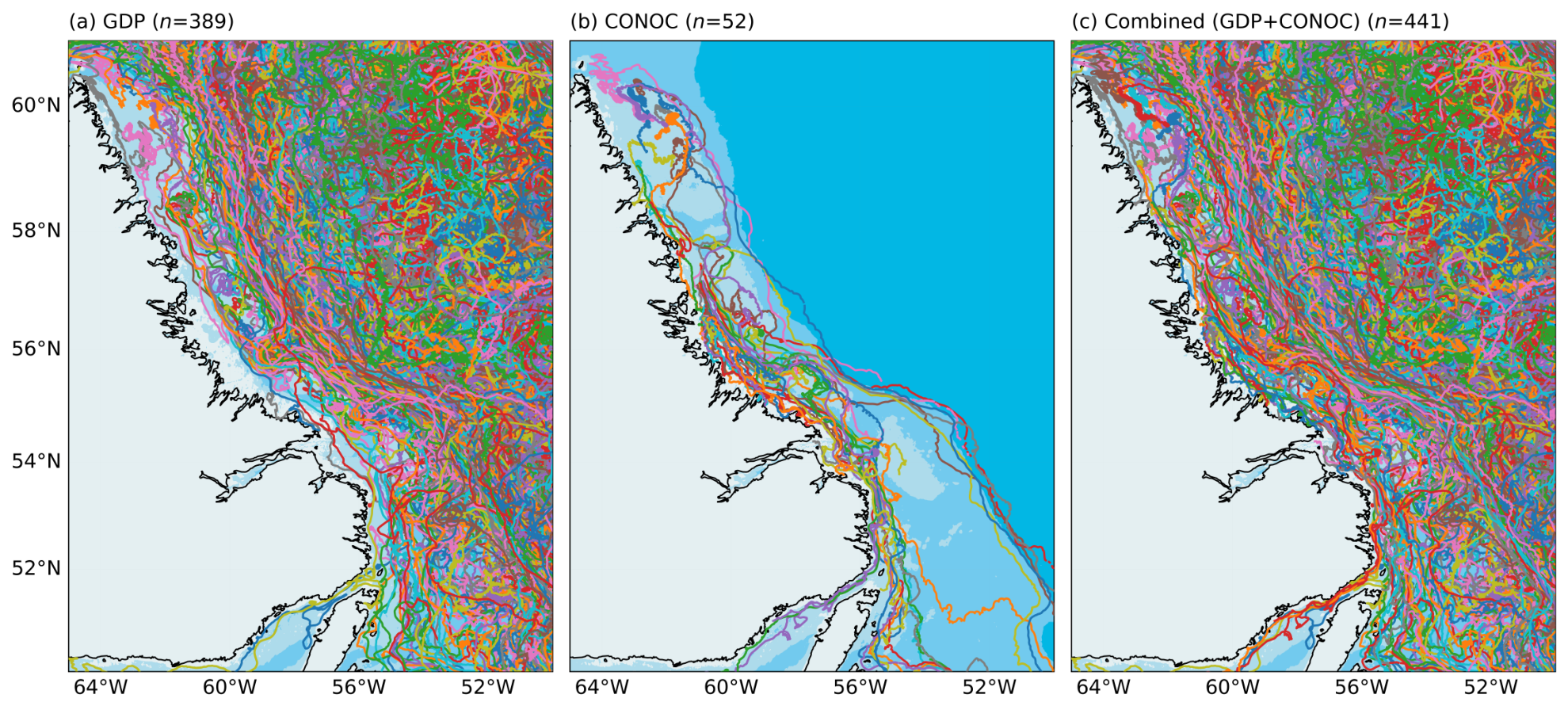
Figure 2. Hourly, quality-controlled drifter tracks from (a) the Global Drifter Program, (b) the Community-based Observations of Nunatsiavut Ocean Circulation project, and (c) the combined dataset. The count (n) in the panel labels indicates the number of drifters in our domain for each dataset.
Jmse 14 01163 g002
Figure 3. Example drifter velocity time series and tidal decomposition. Shown are the total velocity (u, black lines), the tidal component ( u T ) estimated using the Doodson X0 filter (red lines), and the non-tidal component as a residual ( u NT ; blue lines). The three drifters shown are examples of each drifter type: (a) CODE, (b) SVP and (c) CARTHE. The unique International Mobile Equipment Identifier (IMEI) number for each drifter is listed in the panel title.
Jmse 14 01163 g003
Figure 4. Density of gridded drifter data. Counts of drifter data points falling within each 0.25° grid cell for (a) GDP, (b) CONOC, and (c) the combined dataset.
Jmse 14 01163 g004
Figure 5. Tracks from glider missions along the Beachy Island AZMP line. Shown are the Beachy Island AZMP line (black line; stations indicated by black dots), the tracks from the 2020 and 2021 Slocum glider missions (blue and magenta lines respectively), and the tracks from CONOC and GDP drifters (gray lines). The ( x 1 , x 2 ) coordinate system is defined with its origin at the first Beachy Island AZMP station, x 1 oriented positive along the Beachy Island line, and x 2 oriented positive perpendicular to this line.
Jmse 14 01163 g005
Figure 6. Temperature and salinity from the 2020 and 2021 glider transects. The top panels (a,b) show the multiple transects made by each glider (x axis is distance along the Beachy Island line, y axis is month/day). The remaining panels show the temperature and salinity data from the (cj) 2020 and (kr) 2021 Slocum gliders. Black contours show potential density in 0.5 kg/m3 increments with the thick black contour indicating 1027 kg/m3. The gray shaded area shows GEBCO bathymetry interpolated to the glider transect line.
Jmse 14 01163 g006
Figure 7. Gridded ocean currents. (a) Mean tidal ( u T ) current speed. (b) Mean non-tidal ( u NT ) current speed (colors) and direction (arrows). (c) Difference in speeds ( u NT u T ). The Beachy Island AZMP transect is indicated by the dashed blue line.
Jmse 14 01163 g007
Figure 8. Transects of velocity and density along the Beachy Island AZMP line (Figure 5). (a) Velocity in the x 2 direction from the CONOC and GDP drifters (black line), from the July–September mean 2020–2021 GLORYS velocity field at 1.5 m and 15 m depths (dashed and dotted blue lines respectively), and surface velocity due to thermal wind shear, referenced to velocity at the bottom, calculated from the 2020–2021 July–September mean GLORYS density field (red dashed line) and from the gridded, combined glider density field (red solid line). (b) Mean 2020–2021 July–September potential density field (black contours) and velocity in the x 2 direction (colored shading) from GLORYS. (c) Combined glider potential density field (black contours) and velocity due to thermal wind shear, referenced to velocity at the bottom, in the x 2 direction (colored shading). GEBCO bathymetry interpolated onto the transect line is shown in gray in (b,c).
Jmse 14 01163 g008
Figure 9. Baroclinic and barotropic decomposition of Labrador Current System surface velocities along the Beachy Island line. (a) Surface velocities from the combined drifter dataset (representing the total velocity; black line), from the glider-derived thermal wind shear referenced to the velocity at the bottom (representing the baroclinic component; red line), and the remainder (representing the barotropic component; blue line) oriented perpendicular to the Beachy Island line. (b) Proportion (as percent) of total velocity taken up by the baroclinic and barotropic components (red and blue shaded areas respectively) along the Beachy Island line.
Jmse 14 01163 g009
Figure 10. Watermass properties in the LCS over the Labrador Shelf. (a) Three regions (LCC, mid-shelf, and MLC) defined in the x 1 -z plane along the Beachy Island line. Hatching indicates areas where velocities u 2 BC (thermal wind shear referenced to the bottom) are at least 3 cm/s. GEBCO bathymetry interpolated onto the transect line shown in gray. (bd) Temperature–Salinity plots from the glider data for each of the three regions, where color indicates depth and marker size indicates u 2 BC . Gray dots indicate data for all regions.
Jmse 14 01163 g010
Table 1. Volume T V , heat T Q and freshwater transports T F in the Labrador Coastal Current (LCC), mid-shelf region (Mid), and Main Labrador Current (MLC). The two calculations of freshwater transports represent two different reference salinities S 0 (reported in the table as practical salinity).
LCCMid-ShelfMLC
T V (Sv)1.341.636.51
T Q (PW)1.511.837.38
T F (34.8) (mSv)89.091.8166
T F (35.0) (mSv)96.1101203
Disclaimer/Publisher’s Note: The statements, opinions and data contained in all publications are solely those of the individual author(s) and contributor(s) and not of MDPI and/or the editor(s). MDPI and/or the editor(s) disclaim responsibility for any injury to people or property resulting from any ideas, methods, instructions or products referred to in the content.