Influence of Swash Dynamics and Wave Spectral Structure on Beach Cusp Geometry

Abstract

Beach cusp geometry arises from coupled hydrodynamic and morphodynamic feedback in the swash zone. This study used the numerical model XBeach in nonhydrostatic mode to examine cusp development on an idealized sandy beach forced by monochromatic, bichromatic, and band-limited irregular waves. Simulations systematically varied foreshore slope (tan β = 0.05–0.15), wave period (8–12 s), and wave height (0.4–0.8 m), while grouped and irregular cases isolated the effects of infragravity modulation and spectral bandwidth. Under monochromatic forcing, cusp spacing increased primarily with wave period and foreshore slope, whereas wave height played a secondary role. Cusp spacing scaled strongly with horizontal swash excursion, supporting self-organization. Grouped and band-limited forcing increased shoreline excursion but weakened the direct proportionality between cusp spacing and swash excursion, indicating the temporal organization of forcing modulated pattern evolution. Across monochromatic, bichromatic, and irregular cases, spectral diagnostics did not show dispersion-aligned energy consistent with edge-wave forcing. The results support the interpretation of beach cusps as predominantly swash-driven, self-organized features whose geometry is controlled by slope and incident-wave timescale and modulated by spectral structure.

1. Introduction

Beach cusps are crescent-shaped features that sometimes form near the shoreline of sand or gravel beaches. Cusp shape is identified by landward concave embayments and seaward horns. Cusp formation and evolution arise from complex feedbacks between waves, currents, and morphodynamics with variations also depending on grain properties and beach slope.

Low-energy, narrow-banded, shore-normal wave conditions over sandy to cobble beach slopes are some of the typical characteristics that lead to cusp development [1,2]. Cusp morphology measurements used to obtain spacing (horn to horn distance) and relief (vertical distance from horn to embayment) have been gathered through traditional GPS surveying [3,4,5], photogrammetry from fixed [6] and unmanned [7] platforms, and, more recently, the use of lidar technology [8,9,10]. Cusp spacing depends on the geomorphic and hydrodynamic conditions [6,9,11,12] and may reach 50 m or more [8,13,14].

Cusp spacing tends to increase with wave period [15,16,17,18,19], which is mostly consistent with the idea that longer period forcing causes longer alongshore length scales through higher swash excursions and low frequency motions. Tidal variations can also influence cusp shape [10]. For example, rising tides deposit sand in embayments, whereas falling tides tend to erode embayments [10,20,21].

Wave height under moderate-energy conditions often increases the cross-shore cusp excursion and vertical relief as it directly affects sediment mobilization and the magnitude of transport gradients in the swash zone [22,23]. However, this effect may not hold under high-energy conditions like storms that can eliminate cusps by producing highly turbulent and irregular swash that suppresses persistent alongshore structure [4,13,24,25]. In low-energy situations, cusps may not be present or their characteristics length and relief scales are small. The lack of robust morphologic signature is due to weak swash motions unable to transport significant sediment volume [4,15,26].

The frequency structure of the incoming wave field, which can range from monochromatic (laboratory), narrow-band, and broadband forcing to strongly grouped wave conditions, might affect the development of beach cusps because it determines how the timescale and organization of swash-driven transport gradients [15,27]. Low-frequency (infragravity) spectral energy can alter the persistence and timing of sediment transport convergence/divergence patterns, whereas broadband forcing can reduce cusp relief. The beach slope has been known to affect cusp formation. Cusps are generally more evident on steeper, reflective beaches and less so on low-sloping, dissipative profiles [23,28,29]. Classical runup theory for regular waves posits that vertical runup elevation is positively associated with beach slope under constant offshore conditions [30]. Field-scale modeling and empirical work similarly show that slope strongly controls vertical exceedance metrics, whereas predictions become less universal if runup is decomposed into frequency components or when forcing is grouped/random and low-frequency motions contribute substantially [31,32,33], consistent with process-based observations of reflective–dissipative swash dynamics and slope-dependent energy dissipation in the swash zone [34,35].

For a given offshore wave forcing, the sign and magnitude of the slope dependence depend on how swash is quantified (e.g., vertical exceedance statistics versus horizontal shoreline displacement) and on the dominant frequency bands controlling shoreline motion. Vertical runup elevations under regular waves typically increase with foreshore slope, whereas horizontal shoreline excursion does not necessarily scale as 1/tan β because the shoreline motion reflects the integrated response of incident-band forcing and low-frequency variability [36,37,38]. These observations motivate a careful distinction between vertical runup elevation and horizontal swash excursion when interpreting slope effects on cusp morphology, as steeper slopes can limit cross-shore cusp excursion even if cusp relief increases due to stronger focusing and larger gradients in the swash zone [12,23,24]. Although vertical and horizontal measures are geometrically related on a planar beachface, the swash forcing differs fundamentally between reflective and dissipative states, so slope effects can differ depending on the chosen metric [36,37]. Experimental comparisons of bore-driven swash across slopes similarly show that mild slopes tend to produce larger horizontal excursions, while steep slopes cause greater vertical runup, showing geometric and hydrodynamic differences in shoreline response [39]. Together, these results indicate that steeper beaches can favor larger vertical runup while horizontal excursion may decrease for bore-scale or event-scale swash on some profiles, and that under sustained regular-wave forcing, the shoreline-displacement time series can also be shaped by reflection, setup, and nonlinear energy transfers.

Laboratory studies further indicate that shoreline response under bichromatic forcing depends on the slope and nature of the low-frequency motion. Baldock et al. [40] showed that bichromatic forcing can generate low-frequency-dominated shoreline oscillations over reflective to intermediate slopes, while on very mild slopes, the response may remain more strongly bound to the group frequency with substantial interaction between incident and infragravity bands. Here, the group frequency refers to the beat (envelope) frequency imposed by the bichromatic wave pair (Δf = |f₁ − f₂|), whereas low-frequency motion refers to the broader infragravity/long-wave band generated by nonlinear interactions and swash processes and is not restricted to that single imposed frequency. Complementary flume experiments by [41], which examined slopes of 1:10, 1:20, and 1:40, indicated that swash patterns and the relative importance of low-frequency energy depend strongly on slope. Large-scale laboratory studies show that shoreline response under bichromatic forcing is strongly affected by the interaction between incident and low-frequency motions, which can reorganize swash motions and shoreline variability [42]. Collectively, these results indicate that infragravity forcing can obscure simple slope–excursion relationships, particularly for horizontal swash metrics.

The process of beach cusp formation is often discussed in relation to two potential mechanisms: edge-waves and self-organization. The edge-wave mechanism [17] suggests that cusps emerge when standing edge-wave patterns cause the nodes and antinodes to align with the horns and embayments, respectively [43]. Laboratory studies have demonstrated that subharmonic edge waves, usually mode zero, are commensurate with cusp observations [44]. However, edge waves have not generally been linked to cusp formation in field settings [6,45,46,47]. In addition, edge waves may not be an expected formation mechanism for cusp formation in the field due to cusp spacing variability and susceptibility to different wave breaker types [46,48].

Feedback loops involving swash motion, sediment transport, and morphodynamics are the foundational principles for self-organization. In the original self-organization models, the swash dynamics were parameterized through simplified rules relating to morphology and transport [11,12]. A simple model and a basic parameterization of sediment transport were used to investigate cusp growth rate and spacing over planar and non-planar planforms seeded with random perturbations. Simulations indicated a dynamical system dependent on the initial perturbation field and the number of swash cycles, where the cusps spacing varied in time. Field data and simulations [7,27,46,49] seemed to corroborate the self-organization mechanism for cusp generation while demonstrating that cusp spacings increase with horizontal swash excursion.

Numerical modeling from parameterized to more sophisticated has advanced the understanding of cusp development. Prior work showed that cusp spacing scales with swash excursion [11,26] and potentially different types of morphodynamic response related to excursion, relief, and cusp spacing [16,23]. A mechanistic explanation is provided by swash circulation over cusp morphology. Masselink and Pattiaratchi [23], based primarily on field observations supported by a conceptual flow model, described horn-divergent and horn-convergent circulation regimes and showed that the ratio of swash excursion to cusp spacing governs whether cusps are reinforced or eroded. This framework explains the tendency for cusp spacing to increase with swash excursion and the substantial scatter observed across sites and conditions. Still, cusp morphodynamics are difficult to reproduce numerically because they rely on sediment transport parameterizations and sometimes simplified hydrodynamics [20].

More recent studies have generated cusp-like features using fluid-dynamical equations coupled with erodible beds. Unlike the earlier models that use simplified rule sets for the self-organization process, these process-based models solve hydrodynamics, sediment transport and bed evolution as coupled components of the morphodynamic system. Dodd et al. [24] simulated cusp development using a 2D nonlinear shallow water model emphasizing the role of swash-sediment feedback and infiltration [50]. The model showed that self-organization could lead to cusp formation and that infiltration, ignored in the original self-organization models [11,12], could be important for sediment deposition at the cusp horns. The XBeach (nonhydrostatic mode) model [51] has also been used to simulate cusp development. Daly et al. [15] noted alternating swash movements that resembled standing edge-wave patterns near the beginning of cusp formation, even though the model was not meant to reproduce edge waves.

Resonant cross-shore processes such as Bragg reflection over successive sandbars can also influence wave transformation on barred profiles. Field observations have shown an order of 20% incident-energy reflection by natural shore-parallel sandbars [52], and recent observations stated sea-swell reflection coefficients up to 0.8 from a steep nearshore bar–trough system [53]. Theoretical and numerical work has extended this to nonlinear Bragg scattering by sinusoidal sandbars [54] and to harbor resonance and breakwater design [55,56]. Hence, they are acknowledged as a possible complication to barred profiles, but the present study focuses on swash zone morphodynamic feedback that determines cusp spacing.

Despite extensive prior work, cusp metrics have not been systematically connected to forcing conditions in a way that separates baseline controls related to wave period, wave height, and swash zone slope from the additional influence of low-frequency modulation associated with wave-group structure and changes in incident-wave frequency bandwidth (from narrow-band to wide-band forcing). Uncertainty also persists regarding whether observed cusps primarily reflect edge-wave dynamics or are better explained by swash self-organization. Consequently, this modeling study addresses cusp spacing and swash excursion variations with swash slope, wave period, wave height, and wave type and addresses the simulation cusps in relation to edge waves or self-organization.

2. Methodology

2.1. Model Description and Numerical Setup

The open-source XBeach model in nonhydrostatic mode (XBeach-NH) was used to simulate nearshore wave propagation, wave breaking, and swash zone hydrodynamics. In this mode, XBeach resolves short-wave propagation and its interactions with infragravity (long-wave) variability [57], enabling representation of runup and swash zone circulation patterns that are essential to cusp development.

Although the hydrodynamics are solved in nonhydrostatic mode, the sediment transport and bed updating follow the standard XBeach morphodynamic formulations derived from depth-averaged (hydrostatic) shallow-water-type concepts, forced by the simulated near-bed flow and wave-related quantities [57]. Sediment transport was computed using the van Thiel-van Rijn equation with bedload only [58], so morphological updating followed from bedload transport gradients by the sediment continuity equation. XBeach-NH has previously been used to reproduce a cusp on natural beaches (e.g., ref. [15]). Waves in XBeach-NH are generated at the offshore boundary. Wave breaking was represented using the depth-limited dissipation model, which computes energy loss due to breaking based on local wave height relative to water depth [57]. This approach follows the classical Roelvink-type parameterization, in which breaking dissipation is activated as waves shoal and steepen nearshore, and the rate of dissipation is controlled by calibration parameters within the model.

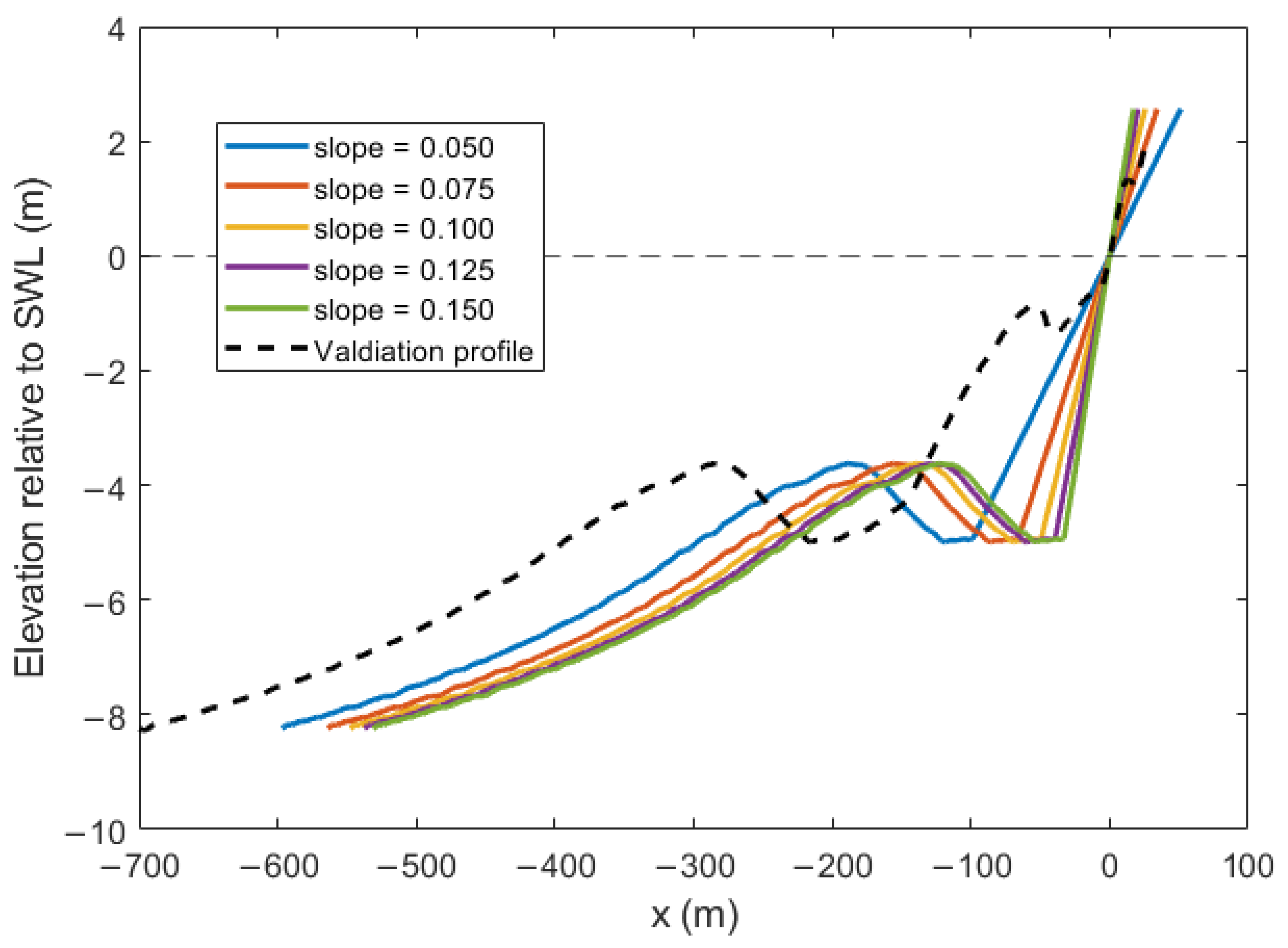
The numerical simulations were conducted using a two-dimensional horizontal (2DH) domain representing an idealized sandy beach. The validation cross-shore bathymetry (Figure 1) was derived from field measurements collected at the U.S. Army Corps of Engineers Field Research Facility (FRF) in Duck, North Carolina, during December 2016 (during the time frame used in O’Dea and Brodie, ref. [9]). The domain extended from offshore at a depth of 8.0 m (relative to still water level; SWL) to a landward position well beyond the initial shoreline, allowing for full capture of swash excursions under wave forcing. The vertical coordinate z is measured positive upward from SWL. The cross-shore profile from profile line 1006 (USACE Field Research Facility; https://chldata.erdc.dren.mil/thredds/catalog/frf/catalog.html, accessed on 26 March 2026) was replicated over a 500 m domain, creating the baseline alongshore uniform bathymetry.

Additional bathymetries were used by prescribing planar foreshore slopes (tan β) that intersect SWL at the shoreline to examine the sensitivity of cusp development to tan β (Figure 1). In these cases, the general offshore bathymetry (including the bar–trough region) was retained, while the inner beach/foreshore region was adjusted to achieve target tan β = 0.05–0.15. Because the shoreline intersection with SWL shifts slightly among slopes, profiles plotted relative to the SWL crossing appear horizontally offset. However, this referencing is used only for comparison and does not alter the offshore boundary forcing.

All simulations used a median grain size of $D_{50}$ = 0.3 mm [59], a sediment density of 2650 kg ${\mathrm{m}}^{-3}$ and a porosity of 0.4. The bottom friction was modeled using the XBeach Manning formulation with a constant roughness coefficient = 0.02 s m⁻¹/³ for all simulations, a standard value for medium-grained sandy beaches. The Courant number was limited to a maximum of CFL = 0.7.

Model configuration included groundwater infiltration, like in previous cusp simulations, removing water from the uprush, which may lead to increased deposition at cusp horns and stronger morphodynamic feedback [15,24]. The selected sediment grain size ($D_{50}$ = 0.3 mm) leads to a relatively low hydraulic conductivity in the groundwater module and, thus, the simulated swash-region profile should be more similar to the weakly permeable or impermeable-beach responses than to the strongly infiltrating cases described by Dodd et al. [24]. Periodic boundary conditions were applied in the alongshore direction to mimic an uninterrupted beach. Grid resolution was held constant across all scenarios at 0.5 m in the cross-shore and alongshore directions. The model time step was dynamically adjusted based on the Courant-Friedrichs-Lewy condition.

Consistent with previous numerical studies of beach cusp self-organization, small random bed irregularities were applied on the beach profile to seed morphodynamic instability. Zero-mean Gaussian perturbations of order 10⁻² m were applied to the swash zone region (about 10% of swash zone cells). These perturbations are uncorrelated in space and do not enforce any preferred alongshore spacing, operating only to trigger the natural growth of instabilities by hydrodynamic sediment feedback. This approach follows the general methodology established by Werner and Fink [12], in which unstable perturbations of a laterally uniform beach initiate self-organization through positive feedback between flow, sediment transport, and evolving morphology, rather than prescribing an initial pattern. Subsequent studies adopted the same principle, seeding models with small random elevation noise on otherwise planar profiles to allow cusp patterns to emerge spontaneously [11,27].

2.2. Wave Forcing and Experiment Design

Monochromatic simulations employed regular (single frequency) incident waves propagating normal to shore ($\theta =0^{\circ }$). The experiment matrix systematically varied tan β, incident wave period (T), and incident wave height (H). The tan β used were = 0.05, 0.075, 0.10, 0.125, and 0.15 (Figure 1). These tan β were combined with T = 8, 10, and 12 s and H = 0.4, 0.6, and 0.8 m. The slope ranges from mildly dissipative to moderately reflective beach states where cusps are commonly observed [23,29] and is consistent with previous numerical cusp studies [15]. The wave height range represents moderate energy cusp-forming conditions [1,2], as higher waves can destroy cusps [25], whereas lower waves may produce insufficient sediment transport over the simulated duration. This monochromatic ensemble forms the baseline dataset used to quantify the relative influence of T, tan β, and H on swash excursion (E) and cusp spacing (λ) under regular forcing.

Free-surface elevation time series were extracted at fixed distances offshore of the SWL crossing (15 m and 25 m offshore) and spectral statistics were computed to check nearshore forcing consistency across the tan β cases. This check was a cross-case numerical verification, not a test for alongshore wave field variation within individual simulations. Across tan β, the dominant peak frequency (and thus (T)) remained identical, while the H varied modestly (about 0.15 m (10–15%) of the target incident H), consistent with local shoaling or reflection differences over the modified inner profile rather than changes to the imposed boundary frequency content.

Bichromatic simulations following established laboratory and numerical studies [40,41,42] imposed two closely spaced incident frequencies centered on a target peak wave period T_p = 10 s and root-mean-square wave height $H_{rms}$ = 0.6 m with equal component amplitudes. The imposed free-surface signal was defined as: $\eta \left(t\right)=A_1\mathrm{c}\mathrm{o}\mathrm{s}\left[2\pi (f_p-\mathsf{\Delta }f)t\right]+A_2\mathrm{c}\mathrm{o}\mathrm{s}\left[2\pi (f_p+\mathsf{\Delta }f)t\right],$ where $f_p=1/T_p$, $\mathsf{\Delta }f$is the frequency offset from $f_p$, and $A_2/A_1$ defines the modulation amplitude. The original bichromatic cases used equal component amplitudes $\left(A_2/A_1=1\right)$, producing full deterministic modulation of the wave. The associated infragravity (beat) period, defined as $T_{IG}=1/\left(2\mathsf{\Delta }f\right)$, where $\mathsf{\Delta }f$ is the frequency separation. Three separations were selected to span representative infragravity timescales: $\mathsf{\Delta }f=0.020$ Hz ($T_{IG}=25$ s), $\mathsf{\Delta }f=0.010$ Hz ($T_{IG}=50$ s), and $\mathsf{\Delta }f=0.005$ Hz ($T_{IG}=100$ s). 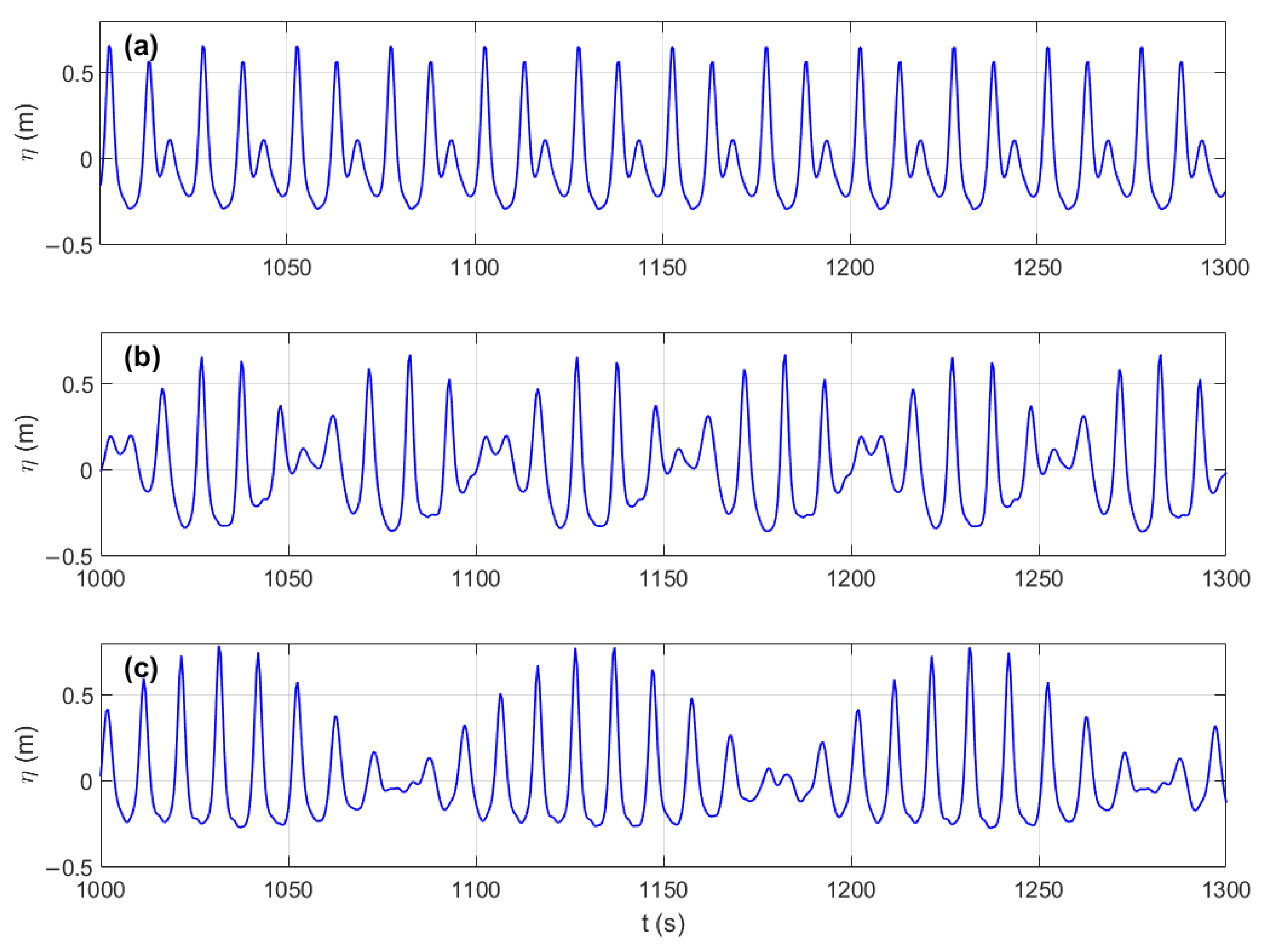These bichromatic cases were designed to isolate how the imposed group modulation timescale alters E and λ relative to the monochromatic baseline. Representative free-surface time series show the resulting wave-group structure (Figure 2).

A second bichromatic set isolated modulation amplitude from group period at fixed group period ($T_{IG}$ = 50 s, $\mathsf{\Delta }f=0.010$ Hz) with modulation amplitude $(A_2$/$A_1$) = 0.25, 0.50, and 0.75. Together with the monochromatic limit ($A_2$/$A_1$ = 0) and the full-modulation case $(A_2$/$A_1$) = 1.0, this set isolates the effect of grouping strength from group period.

Irregular waves forcing using a JONSWAP spectrum evaluated the spectral bandwidth effects. Representative parameters included T_p = 10 s, $H_{rms}$ = 0.6 m, and peak enhancement factor $\gamma$ = 3.3, which controls spectral peakedness in the JONSWAP spectrum. Bandwidth varied by prescribing narrow to wider frequency spreads around the peak frequency, using ranges of ±0.01, ±0.02, and ±0.03 Hz around the peak. These ranges represent narrow-, intermediate-, and wide-band conditions. These simulations support the analysis of how broadband irregularity modifies swash organization and λ.

Free-surface time series were collected just inside the offshore boundary to investigate the wave conditions compared to the prescribed forcing. Water level records were sampled at 1 Hz and de-meaned (temporal mean removed) prior to spectral analysis. Power spectral densities were computed using Welch’s averaged periodogram method with a Hanning window of 2048 samples and 50% overlap, giving consistent frequency resolution and smoothing for all forcing cases. The resulting spectra at the offshore boundary showed that the boundary forcing accurately represents the forced wave conditions. Monochromatic simulations showed a single, discrete spectral peak at the target frequency (0.1 Hz). Narrow- and wide-band irregular cases showed spectral broadening centered on the peak frequency, with bandwidths corresponding to ±0.01 Hz and ±0.02 Hz, respectively. Bichromatic simulations displayed two distinct spectral peaks whose separations match the prescribed $T_{IG}$ = 25, 50, and 100 s, confirming correct implementation of deterministic wave-group modulation. These diagnostics indicate that the offshore boundary forcing reproduces the intended monochromatic, bandwidth-controlled, and grouped wave conditions used in the subsequent hydrodynamic and morphodynamic analyses.

2.3. Simulation Duration, Output Strategy, and Stabilization Criterion

All simulation durations were sufficient to capture the growth and maturation of cusp patterns and to allow for λ stabilization. In practice, monochromatic cases typically developed the primary morphodynamic instability by approximately 10 h, whereas bichromatic and irregular (bandwidth) cases required longer simulation times (~20 h). Morphodynamic fields and cusp metrics were saved every 500 s. Hydrodynamic diagnostics used a higher frequency output saved at 1 Hz to support detailed time series and spectral analyses.

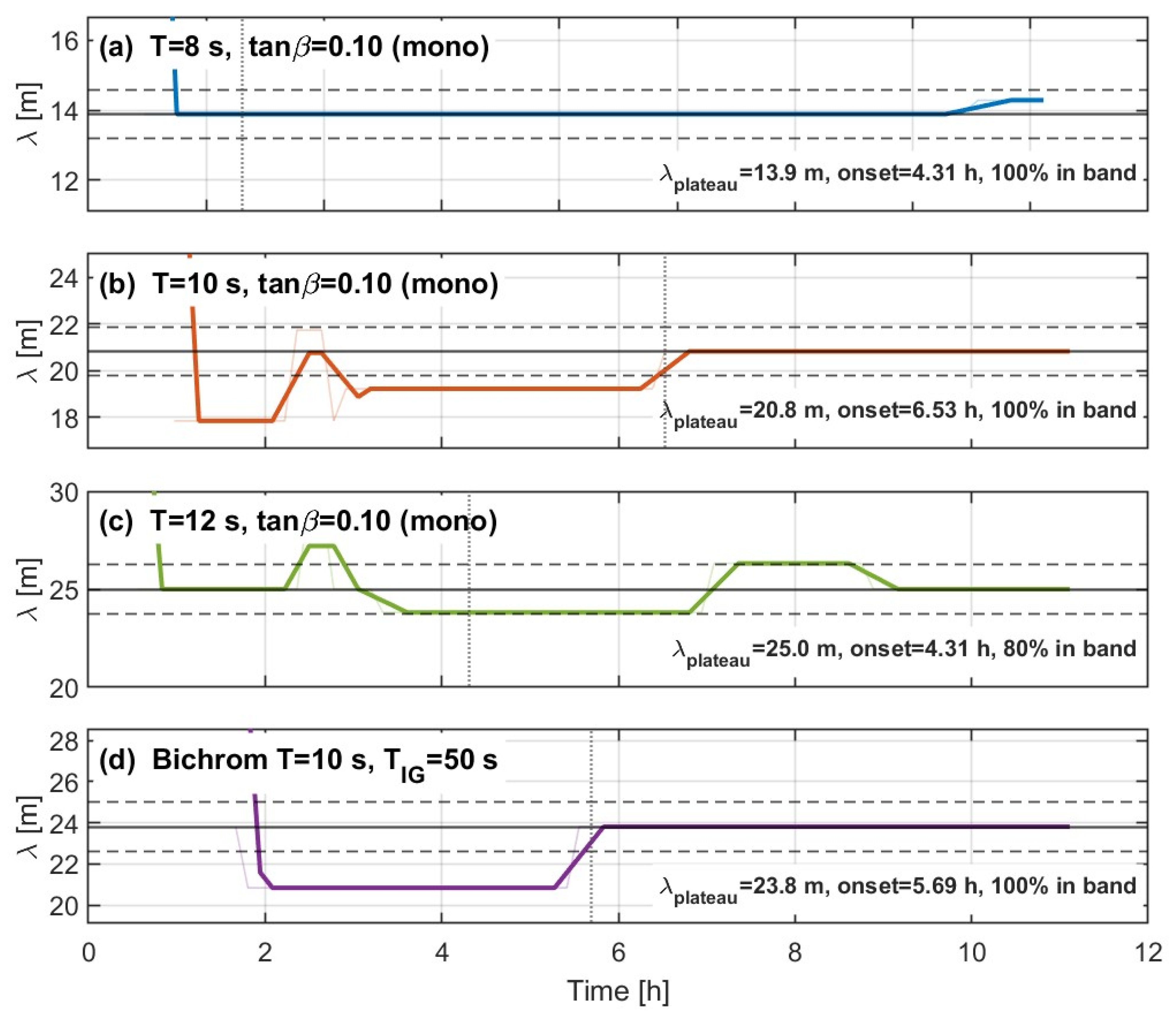
Instead of a strict morphodynamic equilibrium (which does not exist), a quasi-steady cusp spacing-selection based on the time series of λ(t) was quantified. A plateau time was identified as the earliest time when λ(t) remained within ±5% of its mean value over a 1 h window, indicating that λ variability was small relative to the mean. Pattern transitions towards the end of the simulation time (e.g., a change in λ(t) exceeding 5% relative to the plateau mean) were treated as secondary instabilities and used to terminate the analysis window. For four representative cases (T = 8, 10, and 12 s monochromatic, and bichromatic $T_{IG}$ = 50 s, all with tan β = 0.10 and H = 0.6 m), λ(t) was extracted from the FFT of the 0.2 m bed contour at every saved morphodynamic output time. These time series diagnostics are reported in the results sections.

2.4. Measuring Swash Forcing and Cusp Metrics

Swash motion and cusp metrics were measured using the same approaches across all simulations, facilitating direct comparison. Swash motion was characterized using an objective shoreline proxy derived from the model hydrodynamics. At each alongshore location y and output time t, the instantaneous shoreline position $x_s(y,t)$ was defined as the most landward cross-shore location where the instantaneous water depth exceeded a fixed threshold of 0.10 m. This threshold was used to identify a clear shoreline proxy and to avoid numerical noise near the moving wet/dry boundary.

A robust horizontal shoreline-excursion metric E(y) was computed from the time series of $x_s(y,t)$ using a percentile range defined as $E\left(y\right)=x_{s,98}\left(y\right)-x_{s,2}\left(y\right),$ where $x_{s,98}\left(y\right)$ and $x_{s,2}\left(y\right)$denote the 98th and 2nd percentiles over time at each alongshore position. For inter-case comparisons, a single E value was obtained by averaging $E\left(y\right)$across all alongshore grid points, $E=\overline{E} \left(y\right),$ yielding a representative domain-scale E for each simulation while reducing sensitivity to localized alongshore variability (overbar denotes average). This definition obtains the total horizontal shoreline variability, including incident-band swash, swash–swash interaction, and any infragravity contribution, without requiring wave-by-wave runup extraction. This approach follows previous methods for characterizing swash variability from shoreline and runup time series (Coco et al., 2000; Stockdon et al., 2006) [11,38].

Morphological cusp metrics were extracted from the evolving planform using elevation contours referenced to SWL. Cusp initiation was defined as the first time when cross-shore cusp E exceeded 0.70 m at the analysis elevation contour 0.2 m above SWL. The 0.2 m contour was used as a consistent comparative diagnostic. The contour was checked against the $x_s\left(y,t\right)$ percentile envelope and remained within the active swash zone for every tested slope and wave-height combination. λ was estimated from the alongshore variability of the contour-defined planform. For the selected contour elevation, the cross-shore position of that contour defines a planform curve x(y,t). λ was computed as the dominant alongshore spacing associated with x(y,t) using an FFT-based alongshore spectrum. The selected λ corresponds to the spacing at peak spectral energy, representing the dominant alongshore λ. This method provides a consistent and objective λ estimate across all numerical experiments and avoids subjective horn-to-horn selection. λ measures were computed consistently for monochromatic, bichromatic and irregular forcing ensembles.

In addition to λ and E, auxiliary diagnostics were defined to identify comparable growth stages across cases. Cross-shore cusp E based on the fixed elevation contour was defined as the alongshore range in cross-shore position ΔX = max (x(y)) − min (x(y)). Cusp relief A(t) was defined as the vertical difference between horn crest and adjacent embayment trough elevations measured from the bed level profiles at corresponding alongshore location.

Beach cusps are only interpreted as physically meaningful once their relief exceeds background small-scale bed roughness and transient irregularities. Reported cusp vertical relief span a wide range depending on forcing and beach state, from barely measurable to greater than 1 m [22]. Field measurements using repeated topographic surveys similarly show that cusp amplitudes are commonly centimeter–decimeter scale but can reach order 1 m in well-developed cusp systems. For example, Nuyts et al. [7] reported amplitude ranges from 0.04 to 1.05 m across a multilevel cusp field.

2.5. Sensitivity Tests

Several targeted sensitivity tests were performed to evaluate whether the reported cusp-spacing trends depended on profile type, groundwater infiltration, initial bed perturbations, or sediment-transport formulation.

Three additional purely planar profiles without offshore bars were simulated for tan β = 0.05, 0.10 and 0.15 using the same monochromatic baseline forcing (T = 10 s, H = 0.6 m). These simulations were used as robustness checks and tested if the scaling relationships were a result of bar-induced wave transformation.

To explore the effects of infiltration on the barred baseline (T = 10 s, H = 0.6 m, tan β = 0.10), four additional simulations were run with the groundwater flow turned off and hydraulic conductivities of two, five, and ten times the baseline value.

Moreover, three additional simulations with a barred baseline were run to test the sensitivity to the magnitude of perturbation, the imposed spatial structure, and the location of seeding. In each case the baseline forcing was retained (T = 10 s, H = 0.6 m, tan β = 0.10). The first test was performed with the perturbation amplitude reduced by a factor of 10, thus max perturbation = 0.001 m. The second test was similar, but the random perturbation field was replaced by a sinusoidal bed perturbation with an imposed alongshore wavelength = 5 m. In the third test, the cross-shore taper was removed, and perturbations were applied over the whole domain. These simulations were compared with the barred-baseline case to test the sensitivity of the cusp spacing to the initial perturbation field.

Furthermore, one additional sensitivity simulation included suspended-load transport at T = 12 s, H = 0.8 m, (tan β) = 0.10 testing whether suspended load affects the cusp spacing.

3. Results

3.1. Model Validation

The validation simulation was run for 10 h, and wave conditions used in this scenario were informed by field data associated with beach cusp formation at Duck, NC [9] on 9 December 2016 at 1:00 AM UTC. Offshore forcing conditions were Hrms = 0.6 m and T = 9.5 s. Shore-normal, monochromatic waves were selected without introducing variability from spectral or directional spreading.

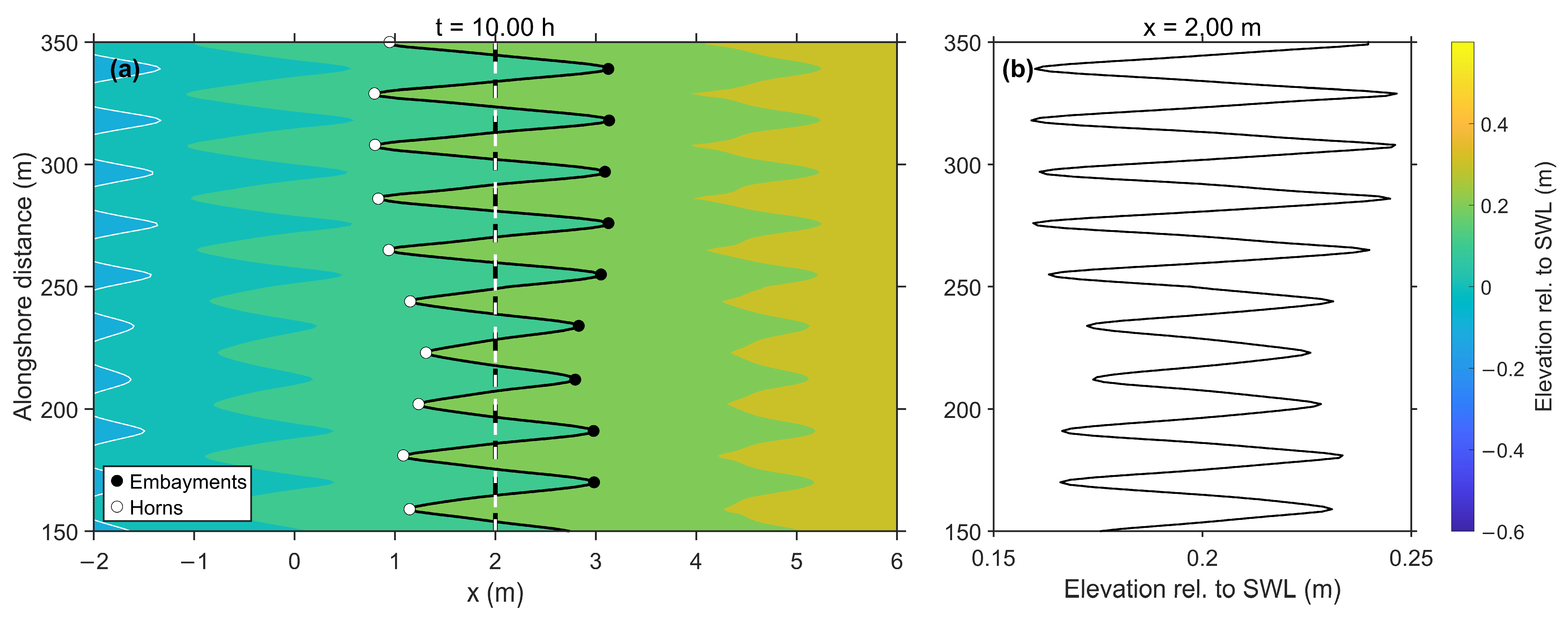
Model performance was evaluated at 10 h and validated with cusp observations from Duck, NC [9]. Two indicators (Figure 3) were identified: λ and cross-shore E. Mean and standard deviation λ were computed from the alongshore distances between successive cusp horns (Figure 3a). The dominant λ was determined independently from alongshore fast Fourier transform (FFT) analysis, while the distribution of horn-to-horn distances provided measures of the λ ranges and their variability. The standard deviation quantifies the regularity of the cusp pattern, with smaller values indicating more uniform λ. Cusp elevation contours from simulations provide visual representations of λ, and growth over time. Contours were extracted relative to SWL at 0.2 m elevation. In contrast, O’Dea and Brodie [9] extracted cusps from the 1.2 m NAVD88 elevation contour, which corresponded to approximately 0.3 m above the observed low-tide level. Because of the monochromatic wave conditions and fixed alongshore profile employed in the simulations, the contour elevations are not directly equivalent. However, both contours are in the active swash region where cusp generation is presented.

The model reproduces cuspate features that mimic those observed in the field [9]. Simulated λ for this monochromatic configuration measured from horn-to-horn distances along the selected contour ranged from 19.3 m to 24 m with a mean λ of 21.59 m, closely aligning with the observed mean λ in the field of 22.2 m and a range of 18.7 m to 24.7 m [9].

Similarly, the modeled contour-based excursion at the 0.2 m contour ranged from 1.26 m to 2.49 m, compared with field-derived contour excursions of 1.15 m to 3.45 m estimated from Figure 10 in O’Dea and Brodie [9]. These values describe the cusp morphology at a specified elevation contour rather than the full three-dimensional cusp excursion. The alignment between model results and observations implies that the numerical setup reproduces beach cusp formation under simplistic forcing conditions and provides a baseline for analyzing morphodynamic response across the idealized scenarios discussed in subsequent sections.

Additional simulations with a 1000 m alongshore domain produced similar results with a mean λ of 21.7 m (range from 19.4 m to 23.8 m) and E ranging from 1.4 m to 2.45 m, suggesting the 500 m alongshore domain was sufficient to capture cusp generation.

3.2. Temporal Evolution of Cusp Morphology

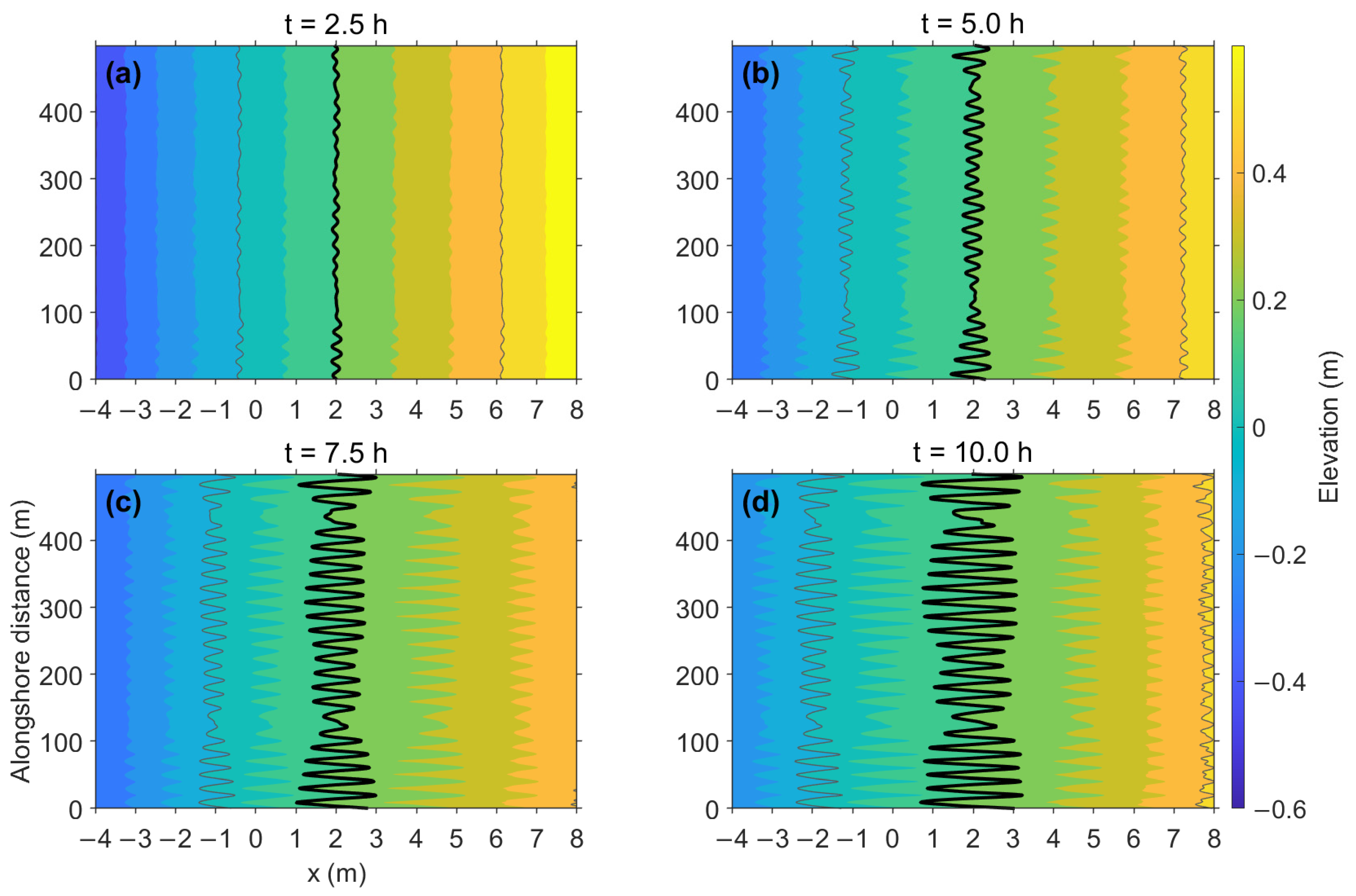
Beach cusp development in the validation simulation emerges from the coupled evolution of wave transformation, swash dynamics, and sediment transport over different bathymetric configurations. The early development of cusps is illustrated through a sequence of elevation contours at successive time steps (Figure 4a–d). At t = 2.5 h (Figure 4a), small-amplitude alongshore cusps are already visible within the swash zone, indicating the onset of instability from initially near-uniform conditions. By t = 5 h (Figure 4b), cusp horns and embayments become clearly identifiable, with increasing cross-shore E of the shoreline contour. At t = 7.5 h (Figure 4c), cusp morphology exhibits larger E and amplitude, together with increased alongshore irregularity as individual cusps interact. By t = 10 h (Figure 4d), cusp horns and embayments are more pronounced, with cusp vertical relief reaching approximately 0.1 m. At later stages, cusp horns develop small-scale irregularities, likely associated with intensified local sediment transport feedback and interactions between adjacent cusps. Despite this complexity, the dominant cusp λ remains similar over time.

For the validation case shown, cusps evolve toward a mean λ of 21.59 m, with a standard deviation of 2.34 m. The relatively small spread (~10%) indicates that the system selects a preferred λ early in the evolution, which is subsequently maintained as cusps mature.

Domain and swash zone sediment budgets verified that cusp evolution reflected physically consistent redistribution of sediment. Alongshore-mean profile evolution was examined to identify cross-shore adjustments associated with cusp development. Domain-integrated net sediment volume change remains very small throughout the simulation. At t = 10.0 h, erosion volume is 2461.1 m³ and deposition volume is 2460.8 m³, giving a net change of only −0.3 m³, corresponding to an imbalance of 0.01%, which is negligible relative to the cumulative erosion or deposition volumes, indicating that cusp evolution is not driven by non-physical mass gain or loss.

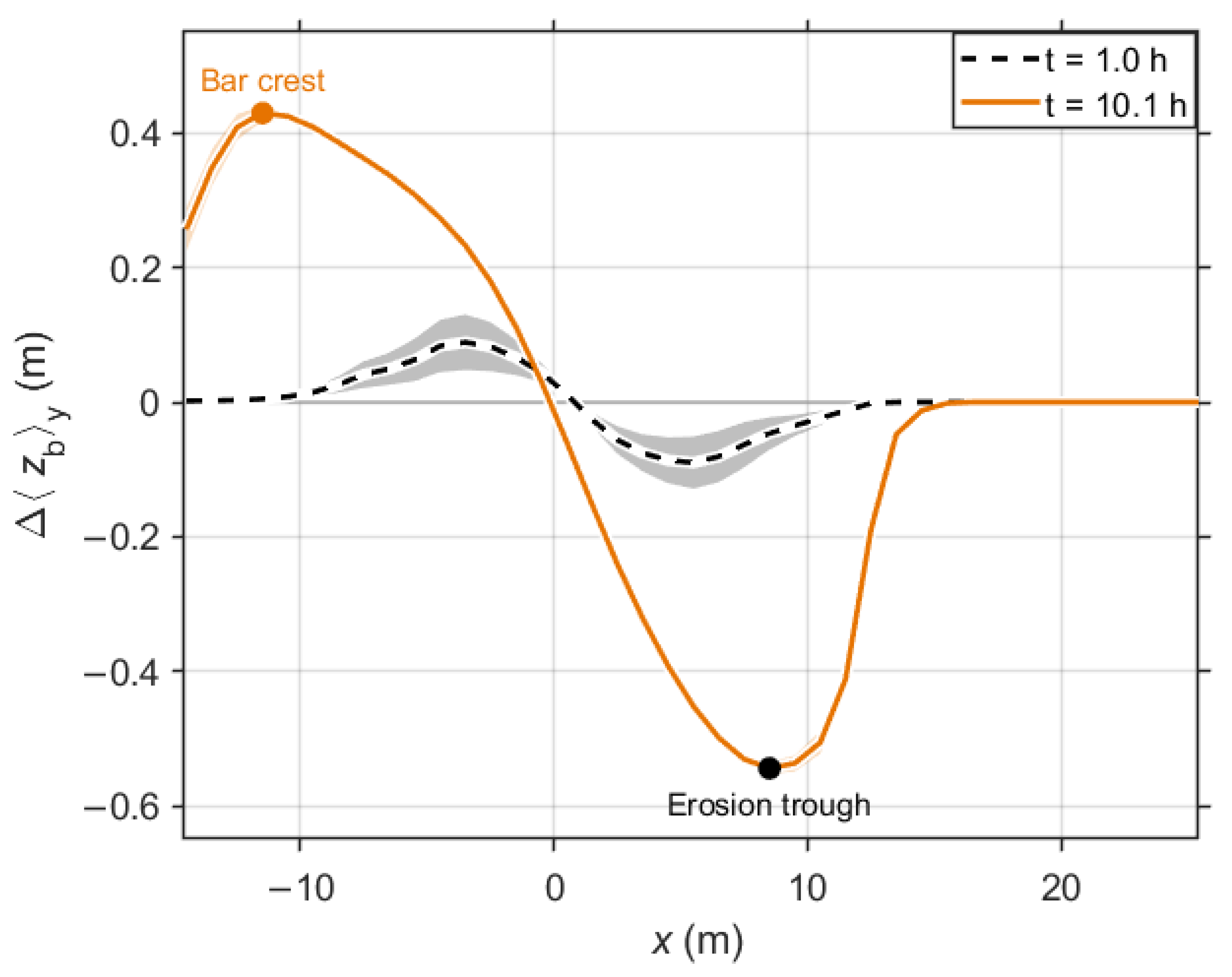
Alongshore-averaged bed elevation was calculated as $⟨z_b{⟩}_y(x,t)={\displaystyle \frac{1}{L_y}}{\int }_0^{L_y}{z}_b(x,y,t) dy,$ where $L_y$ is the total alongshore domain length, and changes were referenced to the initial condition, $\mathsf{\Delta }⟨z_b{⟩}_y(x,t)=⟨z_b{⟩}_y(x,t)-⟨z_b{⟩}_y(x,0).$ The mean-profile change shows a depositional crest seaward of the SWL crossing and an adjacent landward erosional trough (Figure 5).

Shading around the curves represents ±1 standard deviation computed from the alongshore-mean bed-level change evaluated over a short time window (seven snapshots at 500 s output intervals) centered on each displayed time. At each cross-shore position x, this standard deviation quantifies how rapidly the mean profile is evolving within that window as wider shading reflects active morphodynamic adjustment, while narrow shading reflects a stabilized profile. The shading is visibly wider at early time (t = 1.0 h), where the bed is actively evolving, and effectively absent at quasi-equilibrium (t = 10.1 h), indicating stabilization of the mean profile. Peak magnitudes reach approximately +0.40 m at the crest and −0.55 m in the trough. This alongshore-mean crest–trough change reflects an alongshore swash bar similar to that reported by Dodd et al. [24] during cusp development.

3.3. Spectral Diagnostics of Edge-Wave Activity and Self-Organization

Frequency–alongshore wavenumber ($f$–$k_y$) spectra of free-surface elevations distinguished edge-wave forcing from self-organization in the modeled cusp patterns. This diagnostic provides a direct test of whether hydrodynamic energy organizes along theoretical edge-wave dispersion curves, as expected under edge-wave control, or remains predominantly alongshore-uniform, consistent with self-organized morphodynamic behavior [60].

Free-surface elevation ($\eta$) time series were extracted from the model output along an alongshore array at a fixed cross-shore location. The primary spectra shown in Figure 6 were computed at x = −20 m from SWL intersection with the beach. Additional spectra were computed at $x=-10$ m and $x=-5$ m to test whether the edge-wave diagnostic depended on cross-shore array location. The sampling frequency was 1 Hz, and the alongshore λ was uniform.

Each alongshore record was de-meaned (temporal mean removed) by removing the temporal mean. Cross-spectral density matrices were then computed using Welch’s averaged periodogram method, averaging with a Hanning window (300 s) and consistent overlap 50% across all cases. From these cross-spectral matrices, two-dimensional $f$–$k_y$ spectra were constructed using conventional Bartlett beamforming [61]. In all cases shown, the Bartlett estimator is presented because it preserves spectral energy in physical units and provides a conservative representation of directional spreading.

Theoretical edge-wave dispersion curves were overlain for modes $n=0$, $n=1$, and $n=2$, based on the linear edge-wave dispersion relation for a planar beach, ${\omega }^2=\left(2n+1\right)g \mathrm{t}\mathrm{a}\mathrm{n} \beta \mid k_y\mid .$ The dispersion curves are plotted symmetrically about $k_y=0$to represent both propagation directions. This diagnostic framework was applied to (i) a synthetic validation case, (ii) monochromatic wave forcing, and (iii) bichromatic (grouped) wave forcing. Both monochromatic and bichromatic cases were done for T_p = 10 s, $H_{rms}$ = 0.6 m, tan β = 0.1, and $T_{IG}$ = 50 s for the bichromatic case.

Before interpreting the model results, the spectral method was validated using a controlled synthetic signal in which edge waves were explicitly imposed. The synthetic free-surface field was generated analytically, independent of XBeach, by superposing edge-wave modes $n=0$, $1$, and $2$ with multiple alongshore wavenumbers, including both positive and negative $k_y$ and with frequencies chosen to satisfy the corresponding dispersion relation. Random phases were used to avoid artificial standing-wave artifacts, and the amplitudes were equalized at a reference cross-shore location. The resulting synthetic signal was then processed using the same Bartlett $f-k_y$ method applied to the XBeach output. 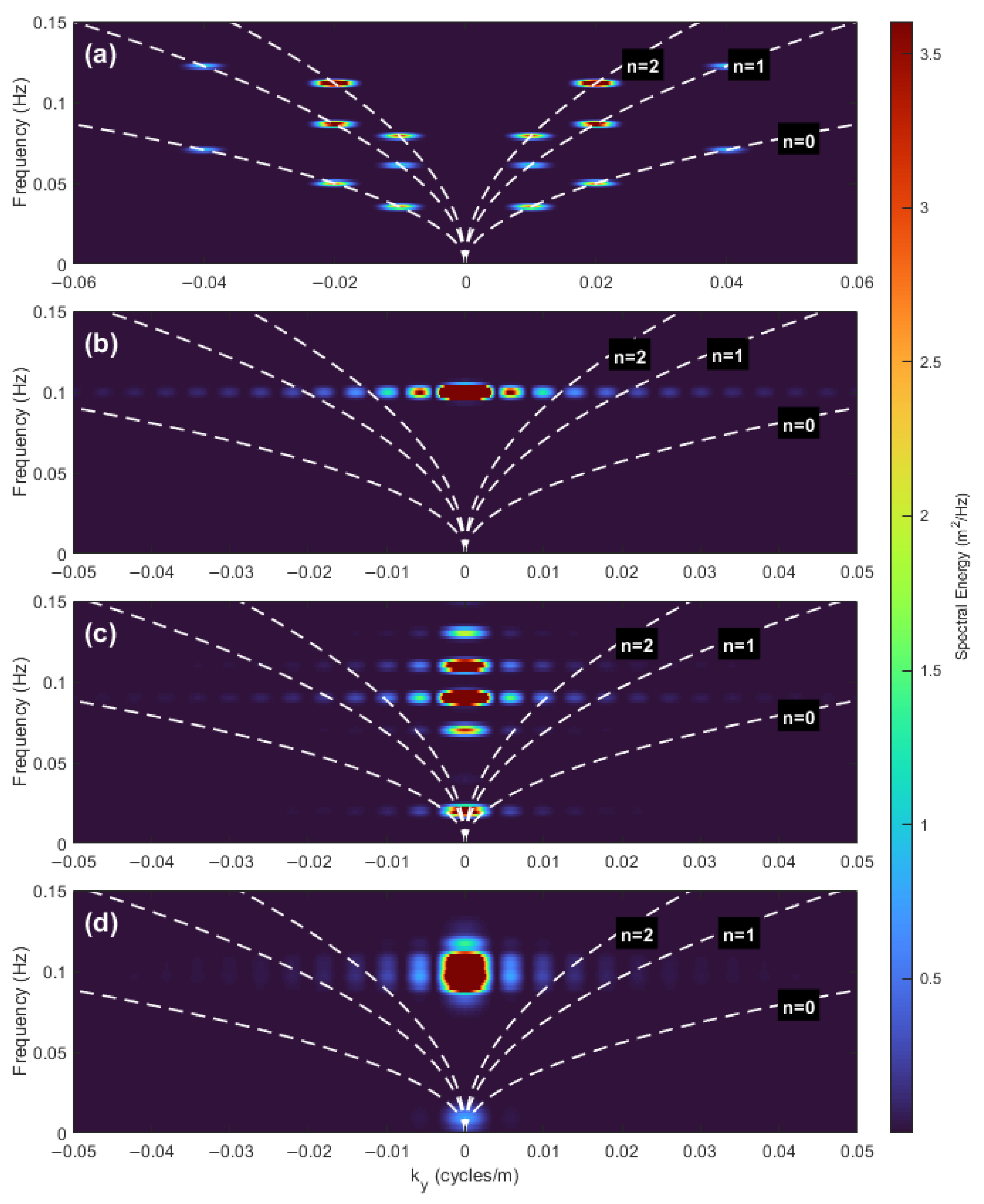Discrete energy maxima in the resulting $f–k_y$ spectrum align closely with the theoretical dispersion curves for all imposed modes (Figure 6a). Energy appears symmetrically about $k_y=0$, consistent with the inclusion of both propagation directions. This indicates that the spectral analysis reliably detects edge-wave energy when it is present and accurately resolves multiple modes and alongshore wavenumbers. For method robustness assessment, the same synthetic signal was processed with additive Gaussian noise at a signal-to-noise ratio (SNR) = 10, 3, 0, and −3 dB. The Bartlett beamformer recovered all three modes imposed at every SNR level. Peak locations agreed with the theoretical dispersion curves in frequency and alongshore wavenumber. This noise test indicates that the lack of dispersion-aligned energy in the XBeach simulations was not caused by insufficient method sensitivity.

Bartlett $f–k_y$spectra for the three forcing cases (monochromatic, bichromatic, and irregular) are plotted using the same color scale to enable direct comparison of spectral energy levels across panels (Figure 6b–d). For the monochromatic forcing case (Figure 6b), spectral energy is concentrated at the forcing frequency band and strongly enclosed near $k_y\approx 0$, indicating alongshore-uniform wave motion. Importantly, no coherent ridge of finite-$k_y$ energy aligns with the theoretical edge-wave dispersion curves for any mode. Small amounts of spectral broadening in $k_y$ near the forcing frequency are attributable to finite array length and windowing effects rather than physical wave propagation. The absence of dispersion-aligned energy indicates that propagating or standing edge waves are not dynamically significant in monochromatic simulations, despite the presence of pronounced cusp morphology.

The bichromatic forcing case (Figure 6c) introduces deterministic wave-group modulation and associated low-frequency (infragravity) variance. The corresponding $f$–$k_y$ spectrum exhibits enhanced low-frequency energy relative to the monochromatic case. However, this energy remains centered near $k_y\approx 0$ and does not align with the theoretical edge-wave dispersion curves. Thus, while infragravity-frequency variance is present under bichromatic forcing, it does not organize into edge-wave modes. This indicates that the occurrence of infragravity energy alone does not imply edge-wave dominance and that grouped-wave forcing does not lead to edge-wave-controlled alongshore structure in the present simulations. The irregular-wave case (Figure 6d) produces broader spectral energy in frequency (as expected for broadband forcing), but the alongshore structure remains dominated by energy near $k_y\approx 0$ without any dispersion-aligned ridges at finite $k_y$. As with the monochromatic and bichromatic cases, the absence of energy concentrated along the theoretical dispersion curves indicates that edge-wave dynamics are not organizing the alongshore variability in the modeled free-surface field for the irregular forcing configuration. Overall, the spectral method successfully identifies edge-wave structure when such waves are explicitly imposed, yet no comparable dispersion-aligned energy is observed in the model simulations.

The cross-shore-location sensitivity test produced the same spectral character at x = −10 m and x = −5 m as at x = −20 m. For monochromatic, bichromatic, and irregular forcing, energy remained concentrated near $k_y\approx 0$, and no coherent finite-$k_y$ ridges aligned with the theoretical edge-wave dispersion curves. The x = −5 m array provides the nearest-shore test, where edge-wave amplitudes would be expected to be larger if cross-shore trapping controlled the response. The absence of dispersion-aligned energy at all tested cross-shore locations supports the interpretation that edge waves were not the dominant organizing mechanism in these simulations.

3.4. Hydrodynamic Support for Cusp Spacing by Self-Organization

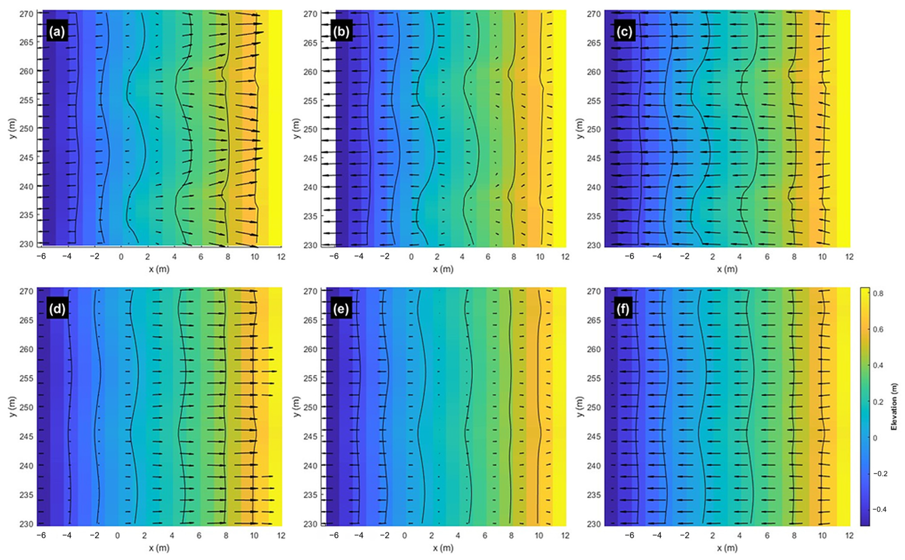
The interpretation of λ selection relies on differences in shoreline forcing, reflectivity, and swash zone circulation feedback between monochromatic and bichromatic waves. Plan-view snapshots present evolving flow and morphology over a fully developed cusp field under monochromatic and bichromatic incident waves (Figure 7).

Both cases use T = 10 s, $H_{rms}$ = 0.6 m, and tan β = 0.1; the bichromatic case includes 50 s wave grouping (group period $T_{IG}$ = 50 s). In all panels, color shading and black contours depict bed elevation (cusp horns as seaward ridges and embayments as landward-recessed troughs), and black arrows denote depth-averaged velocity vectors. All panels share the same color scale and spatial window, enabling direct comparison of morphology and circulation.

Monochromatic forcing produces strong cusp-scale circulation, whereas bichromatic forcing yields more spatially uniform uprush and broader, weaker return flows with reduced hydrodynamic contrast between horns and embayments. Under monochromatic forcing (Figure 7a–c), swash circulation is tightly organized by cusp morphology. During uprush (Figure 7a), onshore flow can be locally stronger near horns, but the uprush also exhibits systematic lateral deflection around the horn toward the embayment center, consistent with divergent flow over horns [6,16,23,62,63].

During the transition phase (Figure 7b), alongshore gradients sharpen as the swash front decelerates, and flow curvature around horns increases, making preferential return pathways through the embayments. By backwash (Figure 7c), return flow becomes strongly focused into narrow offshore paths existing in the embayments, while offshore flow over horns remains weaker and more distributed, indicating net divergence over horns and convergence in embayments at the cusp scale [23]. For the bichromatic case (Figure 7d–f), the alongshore structure of the swash flow is reduced. Uprush (Figure 7d) is more uniform alongshore with weaker cusp-scale variability, and backwash (Figure 7f) still prefers embayments but in broader, less intense flows with reduced horn–bay contrast. This pattern is consistent with grouped forcing generating strong low-frequency shoreline variability and temporal intermittency in swash dynamics, which can weaken the persistence of strong return flows at fixed cusp locations.

Under bichromatic forcing, cusp relief is also reduced, which reduces morphological steering of the swash flow. The weaker alongshore swash structure therefore reflects coupled morphology–flow feedback rather than swash forcing alone. These two effects cannot be separated cleanly in this analysis.

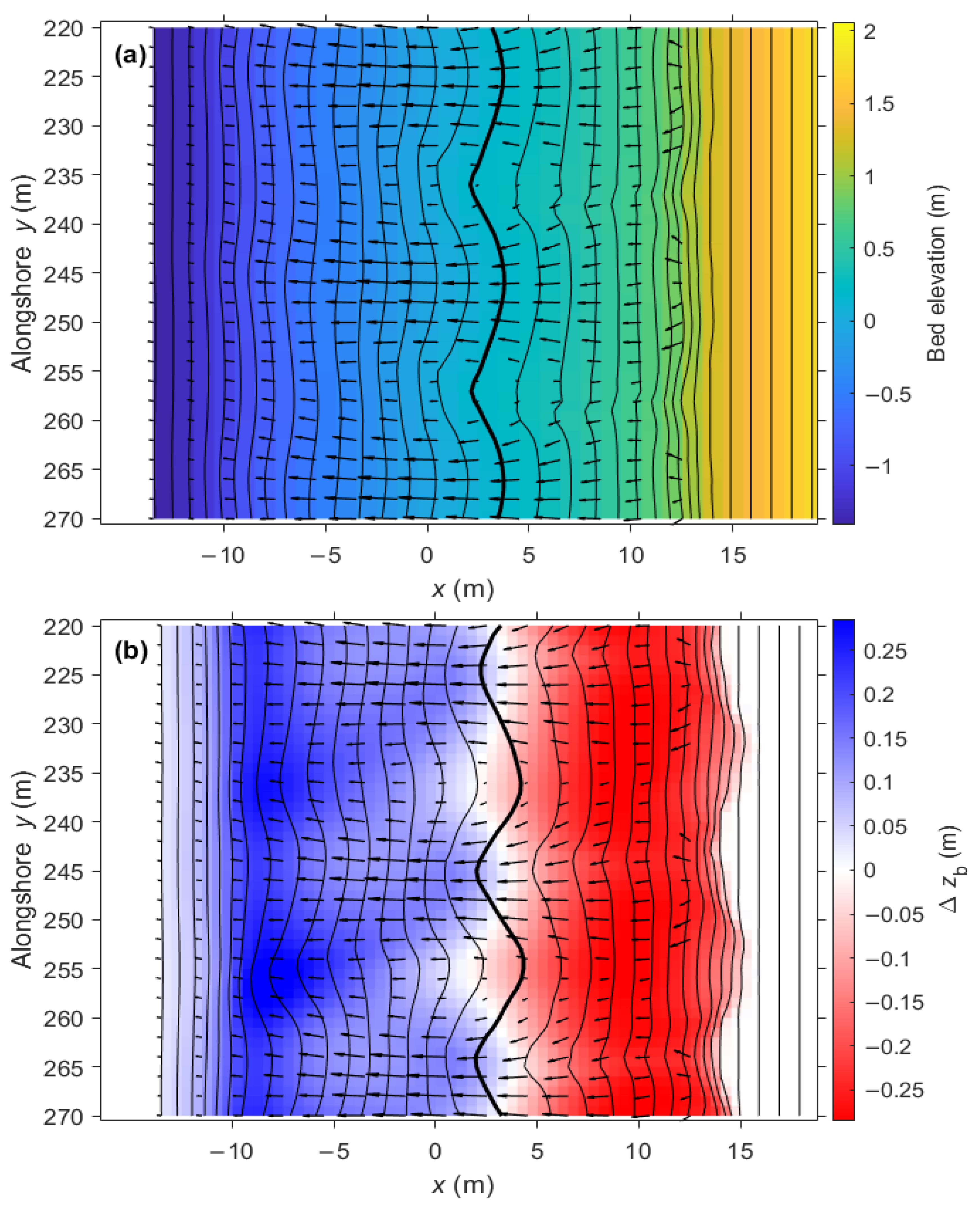
High-resolution outputs for the monochromatic case (T = 10 s, H = 0.6 m, and tan β = 0.1) reveal flow contrasts between cusp horns and embayments, aligning with theories of beach-cusp self-organization. Time-mean depth-averaged circulation velocity fields over developing cusps (Figure 8a) are examined together with cumulative bed-level change (Figure 8b), linking swash circulation, sediment flux divergence, and cusp emergence.

Time-mean depth-averaged circulation shows obvious alongshore periodicity aligned with the cusp form, with flow weakly divergent over horns and convergent within embayments, and the strongest offshore-directed velocities concentrated in embayment paths (Figure 8a). This pattern is consistent with the horn-divergent swash regime in which backwash is channeled through embayments as concentrated return streams, while flow over horns is more laterally distributed [6,16,23,62]. Cumulative bed-level change between the beginning of the simulations (no cusps) and the end ($\mathsf{\Delta }{z}_b$) shows systematic development of cusp relief, with accretion at horns and erosion in embayments (Figure 8b). Focused embayment divergence is consistent with enhanced embayment erosion, while horn accretion indicates net sediment flux convergence under repeated swash forcing.

3.5. Influence of Incident Wave Spectrum on Cusp Formation and Scaling

This section presents the results from the numerical simulations, focusing on how wave forcing parameters (T, H) and tan β across simulations affect E and λ under monochromatic, bichromatic, and irregular wave forcing. Not all parameter combinations produced recognizable cusps within the simulation time. In particular, for the mildest tan β = 0.05 and shortest period at (T = 8 s), no cusps formed for any tested wave height (H or $H_{rms}$ = 0.4–0.8 m). This threshold behavior suggests that wave energy is too weak, and cusp formation requires sufficiently energetic swash motion to overcome diffusive smoothing of the beach profile. These cases are therefore excluded from the subsequent cusp-morphology analysis. Results are organized to show trends and to contrast monochromatic wave behavior with cases involving imposed infragravity modulation.

3.5.1. Monochromatic Wave Forcing

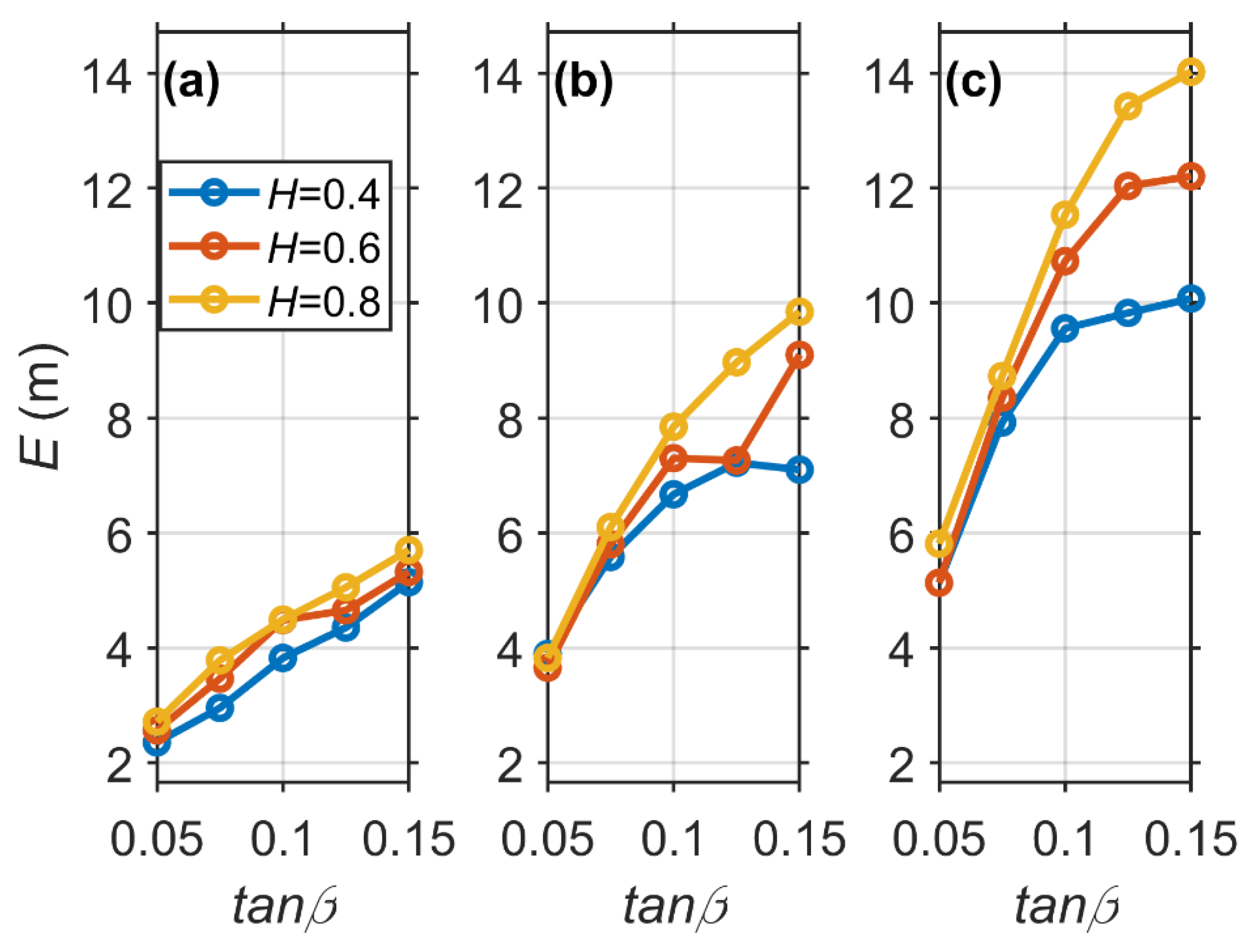
The response of E to tan β under monochromatic forcing was evaluated for three representative periods (T = 8 s, 10 s, and 12 s) and three incident wave heights (H = 0.4 m, 0.6 m, and 0.8 m) (Figure 9).

E increases as tan β increases for all H and T. Larger shoreline displacements for a given tan β are produced by waves with longer T, and this tan β dependence systematically gets stronger with wave period. Beach geometry and incident timescale dominate swash variability under monochromatic forcing, as evidenced by the secondary influence of H, which mainly changes the magnitude of E without changing the overall dependence on tan β. Even though E increases with tan β, the rate of increase tends to taper at the steepest tan β, indicating that E becomes less sensitive as conditions become more reflective. The tan β dependence is illustrated by the reference cases with T = 10 s and H = 0.6 m. Alongshore-averaged values of E increase from 3.7 m for $\mathrm{t}\mathrm{a}\mathrm{n} \beta$ = 0.05, to 7.3 m for $\mathrm{t}\mathrm{a}\mathrm{n} \beta$ = 0.10, and 9.1 m for $\mathrm{t}\mathrm{a}\mathrm{n} \beta$ = 0.15.

This nearly monotonic increase in E reflects the tendency for more reflective beach states to produce larger swash magnitudes under regular forcing. Here, however, E is derived from the horizontal shoreline-position time series and therefore represents the integrated outcome of incident-band uprush, wave reflection, setup, and any model-generated low-frequency variability. As a result, comparisons with studies that report tan β effects on band-limited swash components or single-event bore E should be made cautiously, because differences in forcing regime and E definition can lead to contrasting apparent tan β dependencies. Thus, the increase in $E$ with $\tan \beta$ in Figure 9 should be interpreted as an increase in total horizontal shoreline-position variability, not as a direct measure of swash duration alone. The metric includes incident-band uprush, swash–swash interaction, reflection, setup, and any model-generated low-frequency variability.

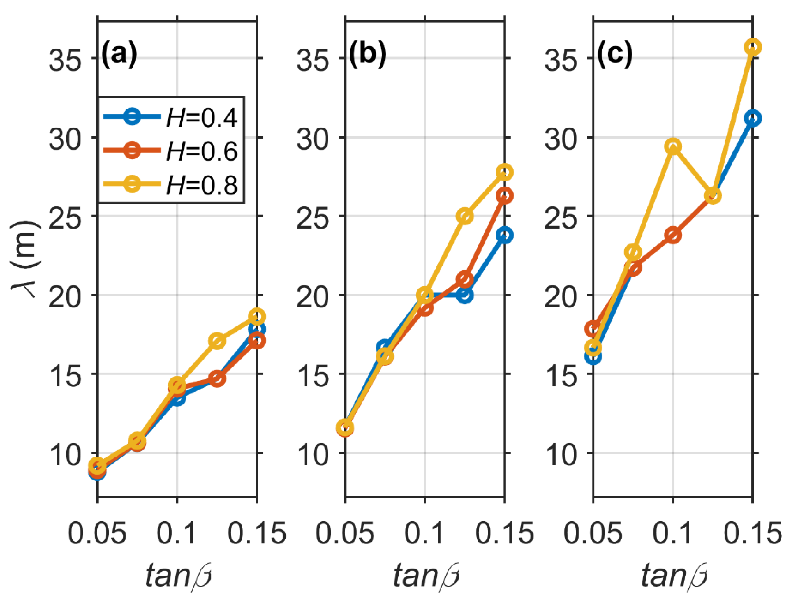
Cusp spacing under monochromatic forcing shows a similarly systematic dependence on tan β and T (Figure 10). For most cases, $\lambda$ increases with $\tan \beta$, and T. Moving from T = 8 s to 10 s to 12 s shifts the $\lambda$ curves upward across the entire tan β range. For example, for T = 10 s and H = 0.6 m, $\lambda$ increases from 16.1 m at $\mathrm{t}\mathrm{a}\mathrm{n} \beta$ = 0.075, to 19.2 m at $\mathrm{t}\mathrm{a}\mathrm{n} \beta$ = 0.10, and 26.3 m at $\mathrm{t}\mathrm{a}\mathrm{n} \beta =0.15$. This trend follows the increase in horizontal shoreline excursion, $E$, rather than swash duration alone, because $\lambda /E$ remains nearly constant across the monochromatic cases.

Figure 10. λ as a function of tan β under monochromatic forcing for three T: (a) T = 8 s, (b) T = 10 s, (c) T = 12 s and three H = 0.4 m, 0.6 m, 0.8 m.

Figure 10. λ as a function of tan β under monochromatic forcing for three T: (a) T = 8 s, (b) T = 10 s, (c) T = 12 s and three H = 0.4 m, 0.6 m, 0.8 m.

In comparison to the dominant T and tan β dependence, H has a relatively small impact on λ, resulting in modest offsets. This behavior implies that rather than determining the preferred alongshore λ, H largely controls the strength of hydrodynamic forcing and sediment mobility. Other XBeach-based cusp simulations have shown similar behavior, with H having a greater impact on cusp development strength than the chosen alongshore λ (e.g., ref. [15]). The $H=0.8$m cases include a local change from the monotonic slope trend, with reduced spacing at the steepest slopes. This behavior is interpreted as a transition in which stronger breaking and nonlinear swash interactions disrupt the dominant cusp mode, so the FFT identifies a shorter alongshore scale. Visual inspection of the bed contours confirmed cusp morphology in the cases used for analysis.

The nondimensional ratio C = λ/E remained nearly constant across tan β (C = 2.6–3.2). This near constancy indicates that, under monochromatic forcing, λ scales directly with a swash-related horizontal length scale, consistent with self-organization frameworks in which λ emerges as a multiple of E or a related runup length scale [12,46].

The monotonic planar profile tests produced similar excursion-based spacing behavior, indicating that the scaling was not an artifact of the barred bathymetry. For T = 10 s and H = 0.6 m, the planar cases at $\mathrm{t}\mathrm{a}\mathrm{n} \beta$ = 0.05, 0.10, and 0.15 produced E = 4.02, 6.88, and 7.93 m and $\lambda$ = 11.9, 20.80, and 27.78 m, respectively. The corresponding $\lambda /E$ ratios were 2.96, 3.02, and 3.50. The planar $\mathrm{t}\mathrm{a}\mathrm{n} \beta$ = 0.1 case differed from the matched barred profile spacing by less than 4%, supporting the interpretation that the $\lambda \sim C/E$ scaling is not caused solely by bar-induced wave transformation.

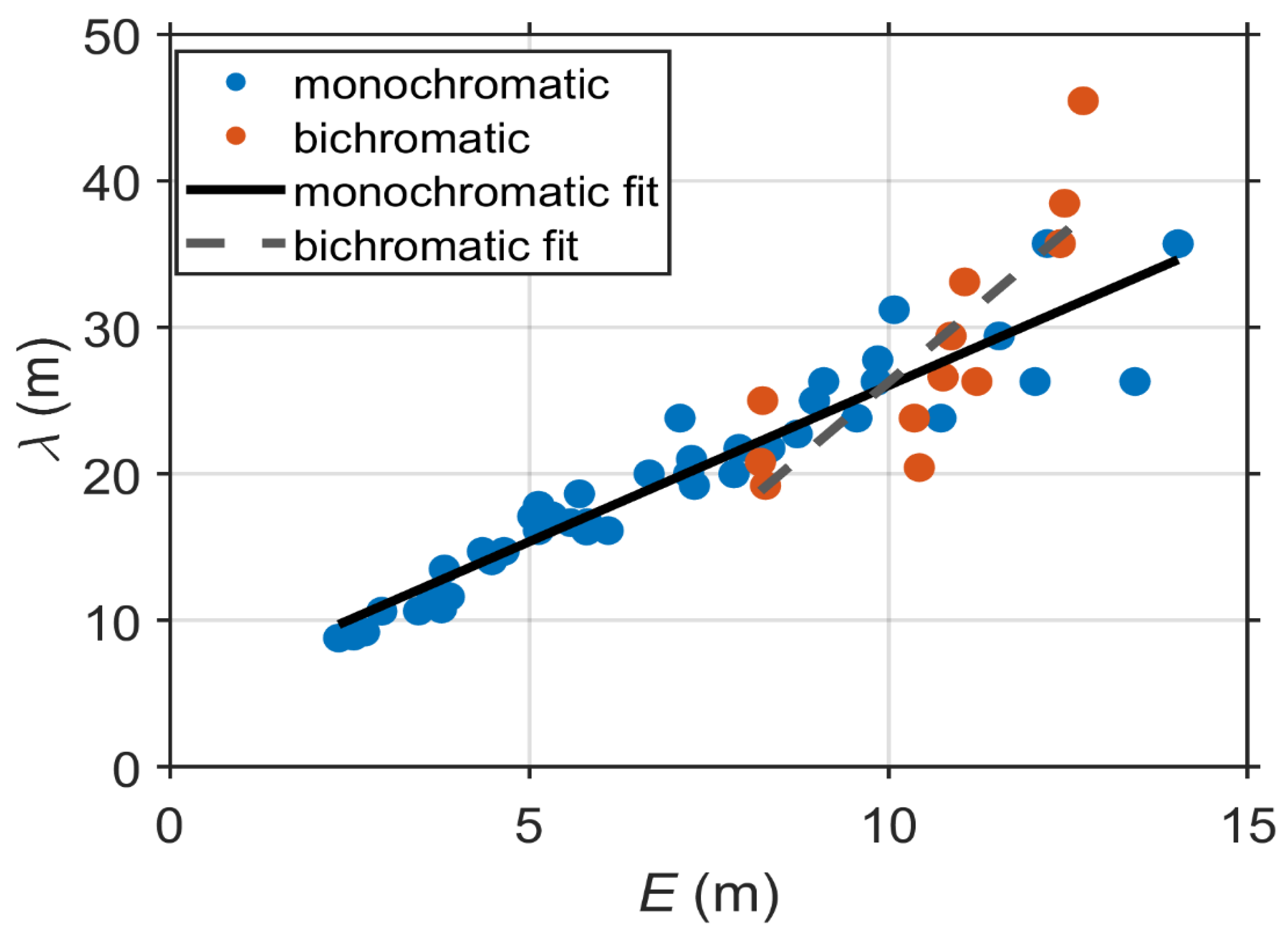
The strong linear relationship between λ and E for monochromatic cases is illustrated by comparing λ against E (Figure 11). A linear fit yields R² = 0.90, indicating that a large fraction of the variance in λ is explained by E alone, similar to previous studies [11,12,46]. Bichromatic cases are also shown in Figure 11 for reference and are discussed in Section 3.5.2.

Standardized multiple linear regression of λ and E using offshore T, tan β, and offshore H as predictors indicates the dominant role of T and tan β. Predictors and responses were z-score standardized (zero mean, unit variance), so regression coefficients are dimensionless standardized beta weights directly comparable across predictors. For λ, the model explains a large fraction of the variance (R² = 0.87; N = 57), with T and tan β identified as the dominant and comparably strong controls (|β(T)| ≈ 0.63, p < 10⁻¹⁵; |β(tan β)| ≈ 0.62, p < 10⁻¹⁵). Offshore H provides no measurable additional explanatory power once T and tan β are accounted for (|β(H)| ≈ 0, p ≈ 0.97), consistent with the weak H sensitivity observed in the λ trends. Because regression uses only three wave heights ($H=0.4$, 0.6, and 0.8 m), it has limited statistical power to resolve a small wave-height effect. The result is therefore interpreted as evidence that wave height explains little additional variance within the tested range, rather than as evidence that wave height has no effect. For E, the model yields R² = 0.83 (N = 57), with T as the strongest predictor (|β(T)| ≈ 0.70, p < 10⁻¹⁵), followed by tan β(|β(tan β)| ≈ 0.53, p ~ 10⁻¹²), and a weaker but statistically detectable influence of H(|β(H)| ≈ 0.12, p = 0.047). Together, λ is primarily controlled by T and tan β, whereas H mainly modulates the magnitude of shoreline motion rather than the selected alongshore λ. Since T and tan β are the two dominant independent controls on λ, the deep-water Iribarren number ${\xi }_0=\mathrm{t}\mathrm{a}\mathrm{n} \beta /\sqrt{H_0/L_0}$ with $L_0=\mathrm{g}{T}_p^2/2\mathsf{\pi }$ and $H_0=\sqrt{2}{H}_{rms}$, provides a natural dimensionless framework that combines both controls and may organize λ more robustly than either parameter alone.

3.5.2. Bichromatic and Grouped Wave Forcing

Under bichromatic forcing, the strong dependence of E on tan β becomes weaker. This behavior is expected because grouped forcing generates pronounced low-frequency shoreline motions whose tan β dependence differs fundamentally from that of incident-band swash [17,64].

Field observations show that the incident-band component of swash can decrease with increasing tan β when swash is decomposed by frequency, whereas infragravity-band motions tend to become increasingly dominant on more shallow sloping beaches, likely because gentler tan β promotes dissipation and suppresses incident-band energy, shifting the swash spectrum toward infragravity frequencies [38]. Because the E metric is computed from the full shoreline-position time series and not band-pass filtered, the tan β dependence here should be interpreted as a control on total horizontal shoreline E rather than on the incident-band component alone, with the relative contribution of infragravity forcing depending on beach state.

For a beat period of $T_{IG}$ = 50 s, $H_{rms}$ = 0.6 m, T_p = 10 s, the alongshore-averaged E shows weak sensitivity to tan β, with $E=10.96$ m for $\mathrm{t}\mathrm{a}\mathrm{n} \beta$ = 0.075, $E$ = 10.36 m for $\mathrm{t}\mathrm{a}\mathrm{n} \beta$ = 0.10, and E = 10.87 m for $\mathrm{t}\mathrm{a}\mathrm{n} \beta$ = 0.15. These weak variations contrast highly with the strong tan β dependence observed under monochromatic forcing and are consistent with previous studies demonstrating that grouped or irregular forcing alters swash dynamics by enhancing infragravity motions [31,36]. Laboratory results further indicate that under long T_p bichromatic forcing, E is controlled primarily by the sequence of short-T_p rather than by the low-frequency group motion itself [42], which reduces geometric sensitivity to tan β when infragravity motions dominate. Consistent with this interpretation, E remains nearly unchanged across variations in H or T_p at a given $\mathrm{t}\mathrm{a}\mathrm{n} \beta$, indicating that infragravity mechanisms dominate over local tan β control in these grouped-wave cases.

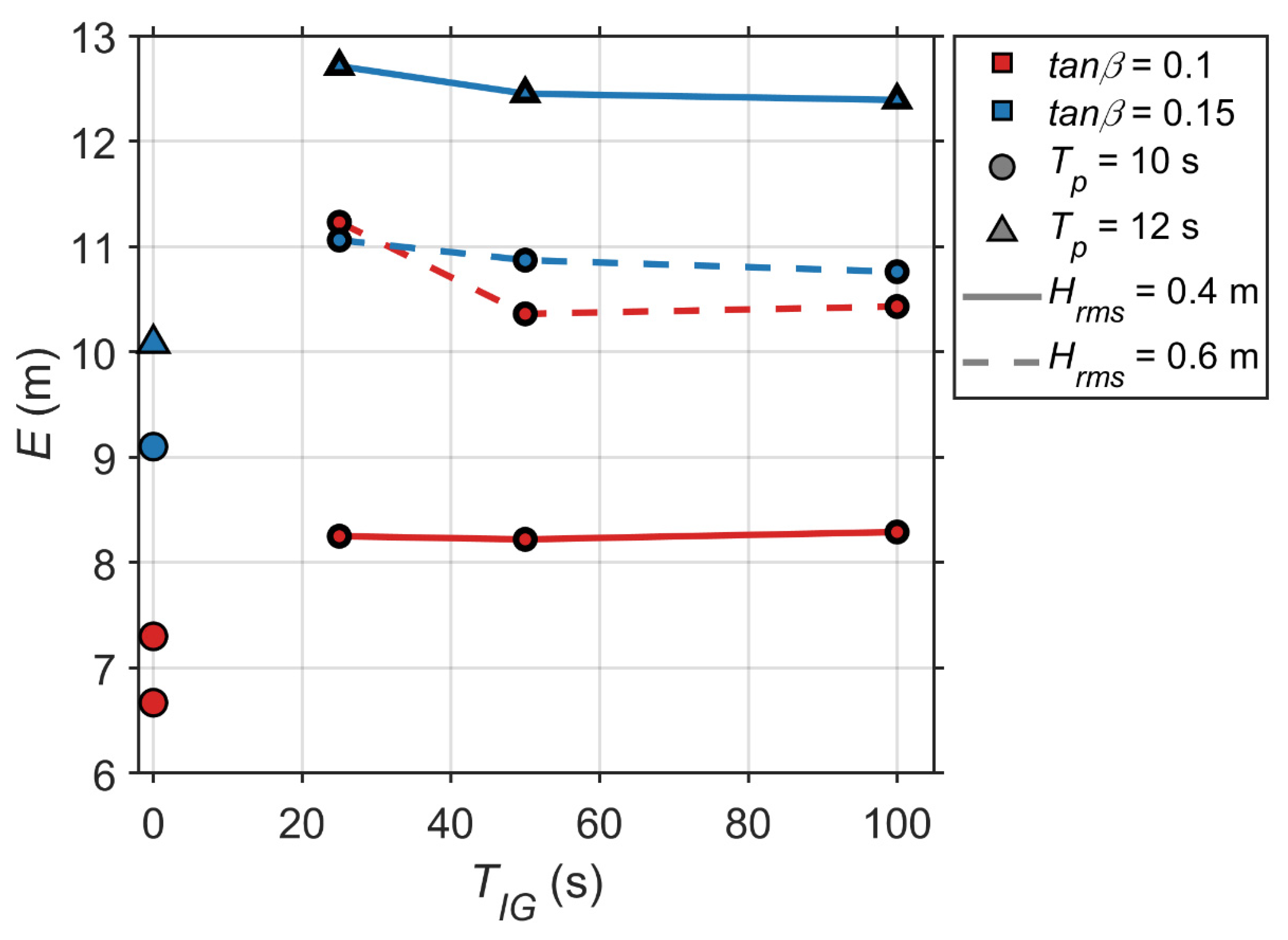
The influence of $T_{IG}$ is further illustrated by explicit $T_{IG}$-series comparisons (Figure 12). For fixed tan β, T, and $H_{rms}$ ($\mathrm{t}\mathrm{a}\mathrm{n} \beta$ = 0.1, $H_{rms}$ = 0.6 m, T_p = 10 s), E decreases modestly as ${\mathrm{T}}_{\mathrm{I}\mathrm{G}}$ increases, from E = 11.23 m at $T_{IG}$ = 25 s to E = 10.36 m at $T_{IG}$ = 50 s and remaining nearly unchanged at E = 10.43 m for $T_{IG}=100$ s indicating that shorter infragravity modulation is more effective at enhancing shoreline motion. A similar but small decrease with increasing $T_{IG}$ is also evident for the added case at $\mathrm{t}\mathrm{a}\mathrm{n} \beta$ = 0.15, $H_{rms}$ = 0.6 m, T_p = 10 s, where E decreases from 11.06 m ($T_{IG}$ = 25 s) to 10.87 m ($T_{IG}$ = 50 s) to 10.76 m ($T_{IG}$ = 100 s).

Cusp spacing responds more strongly than E to grouped forcing. For bichromatic cases with $T_{IG}$= 50 s and $H_{rms}$ = 0.6 m, T = 10 s, λ nearly doubles from $\lambda$ = 15.2 m at $\mathrm{t}\mathrm{a}\mathrm{n} \beta$ = 0.075 to $\lambda$ = 29.4 m at $\mathrm{t}\mathrm{a}\mathrm{n} \beta$ = 0.15, while E remains nearly constant at approximately 11 m. This indicates that, under grouped forcing, alongshore pattern selection is more sensitive to how wave-group modulation structures the swash and nearshore circulation than to changes in total horizontal shoreline E alone (Figure 13).

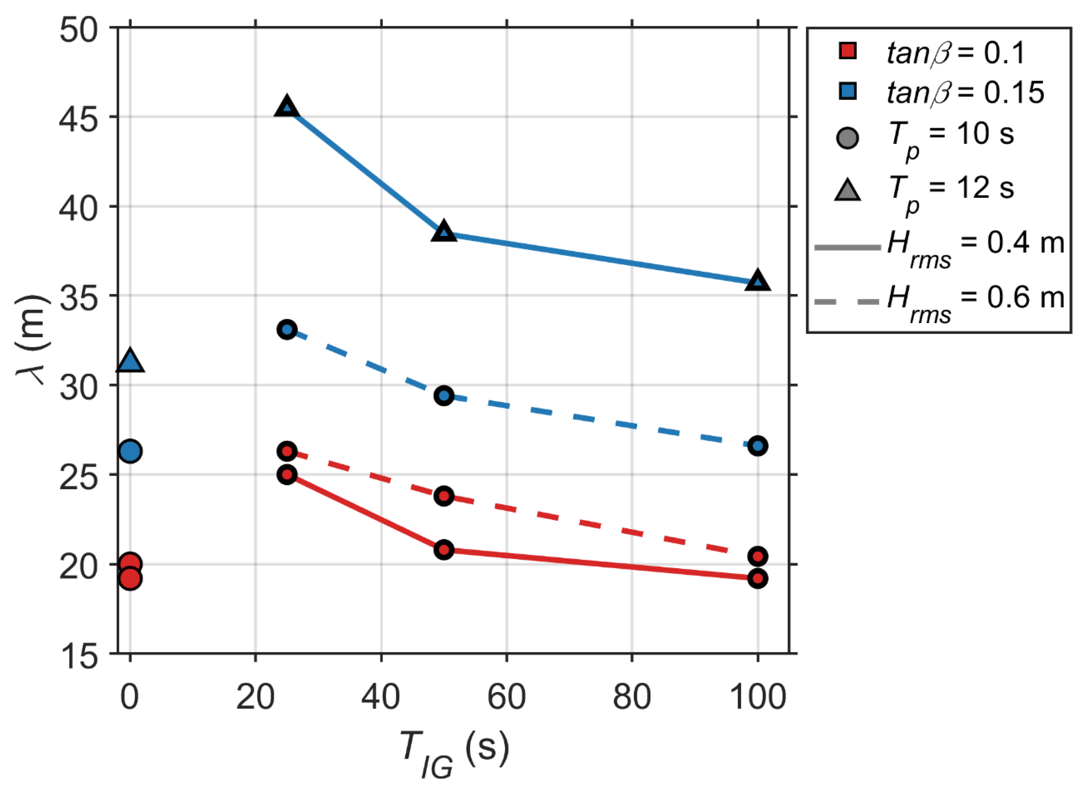
For $\mathrm{t}\mathrm{a}\mathrm{n} \beta$ = 0.1, $H_{rms}$ = 0.6 m, T_p = 10 s, λ increases systematically as $T_{IG}$ decreases, from $\lambda$ = 20.8 m at $T_{IG}$ = 100 s, to $\lambda$ = 23.8 m at $T_{IG}$ = 50 s, and $\lambda$ = 26.3 m at $T_{IG}$ = 25 s. A consistent decrease in $\lambda$with increasing $T_{IG}$is also observed for the case $\mathrm{t}\mathrm{a}\mathrm{n} \beta$ = 0.15, $H_{rms}$ = 0.6 m, T_p = 10 s, where $\lambda$ decreases from 33.1 m ($T_{IG}$ = 25 s) to 29.4 m ($T_{IG}$ = 50 s) to 26.6 m ($T_{IG}$ = 100 s). This increase in $\lambda$ as $T_{IG}$ decreases is physically consistent with self-organization theories in which enhanced low-frequency swash variability promotes larger λ [7,27].

The modulation depth sweep at fixed $T_{IG}$ = 50 s further isolates the effect of wave grouping from group period. Increasing $A_2/A_1$ from 0.25 to 0.50 and 0.75 increased E from 6.42 m to 7.41 m and 8.22 m, respectively. The corresponding $\lambda$ values were 15.15 m, 20.00 m, and 20.83 m. Thus, E increased with modulation depth, whereas $\lambda$ approached a plateau once $A_2/A_1$ exceeded 0.50. The ratio $\lambda /E$ remained near 2.5 across the sweep, indicating that the grouped cases retained an excursion-based spacing scale, but with a weaker sensitivity of $\lambda$ to additional modulation beyond moderate grouping.

The direct impact of infragravity modulation is isolated through paired comparisons between monochromatic ($T_{IG}$ = 0) and bichromatic cases with the same tan β, T_p, and $H_{rms}$ (Figure 12 and Figure 13). E increases consistently under bichromatic forcing for all matched cases, confirming that infragravity modulation systematically enhances cross-shore shoreline variability. In contrast, the response of λ is different as $\mathsf{\Delta }\lambda$ is generally positive for short $T_{IG}$ = 25 s but weakens and may approach zero or become negative as $T_{IG}$ increases. This indicates that infragravity forcing does not entirely increase λ but instead modulates it depending on the relative timescales of swash forcing and morphodynamic adjustment.

3.5.3. Irregular Wave Forcing with Bandwidth Alteration

Frequency bandwidth (spectral spread) modifies wave-group structure and the associated low-frequency forcing that can influence swash dynamics and runup variability (e.g., via group-bound long waves and subharmonic infragravity motions) [40,65,66].

Band-limited irregular waves centered on the monochromatic peak frequency isolated the influence of spectral bandwidth while maintaining a fixed dominant timescale. The monochromatic forcing is defined by $f=f_p$ = 0.10 Hz. The band-limited cases distribute energy within a symmetric interval about $f_p$, with $\mathsf{\Delta }f$ = (0.01, 0.02, 0.03 Hz), corresponding to frequency bands 0.09–0.11 Hz, 0.08–0.12 Hz, and 0.07–0.13 Hz, respectively. All cases shown use the same target $H_{rms}$ = 0.6 m and T_p =10 s and differ only in the spectral bandwidth of the incident forcing.

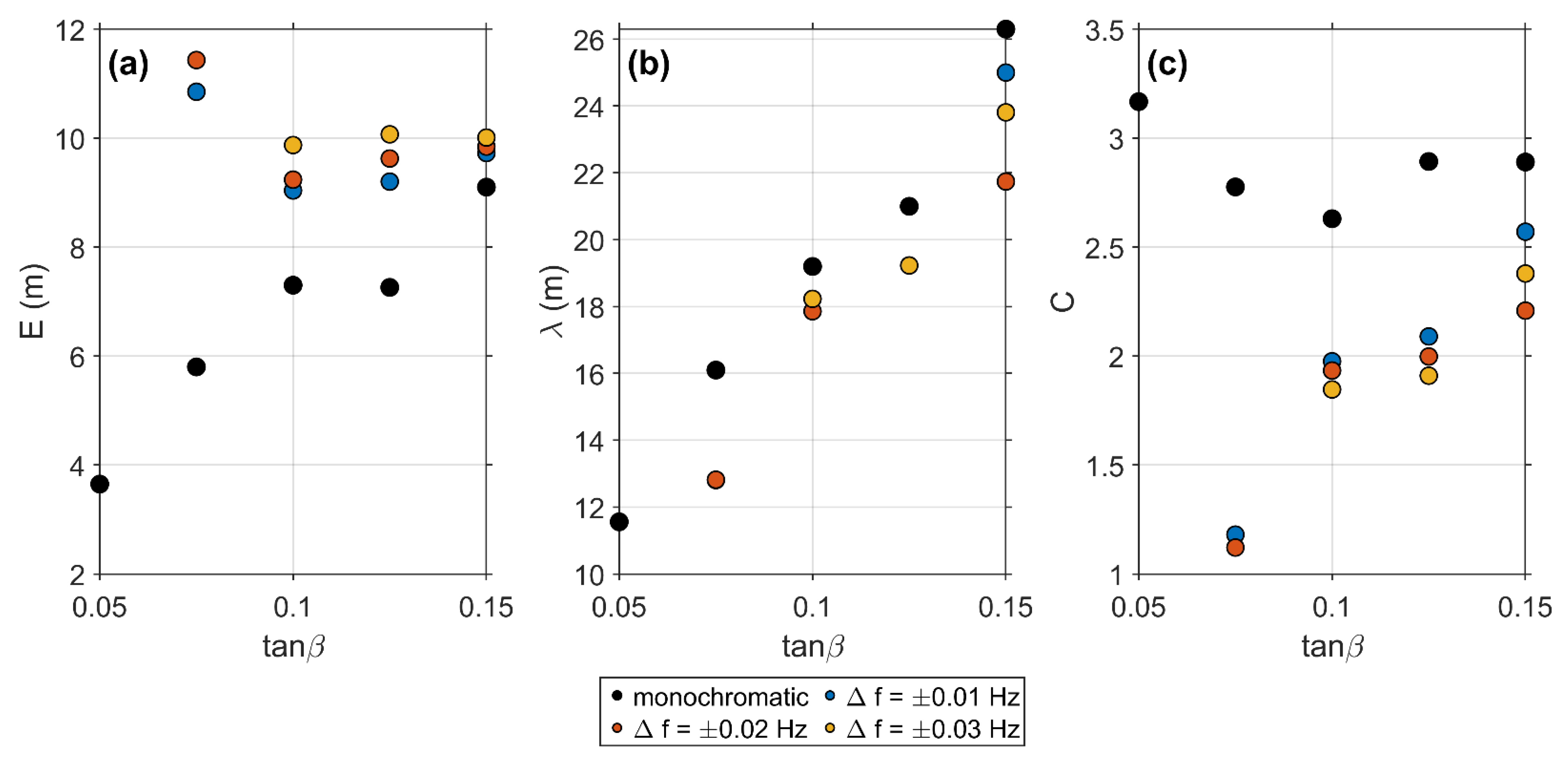
Figure 14 summarizes the response of $E$ and $\lambda$ as a function of $\tan \beta$ for monochromatic and band-limited irregular wave cases. For the monochromatic forcing, both $E$ and $\lambda$ increase with tan β over the tested range (e.g., E from 3.65 m to 9.1 m and λ from 11.65 m to 26.3 m from tan β = 0.05 to 0.15).

Mild tan β (0.05 and 0.075) did not produce cusps for wider frequency bandwidths (0.02 and 0.03 for tan β = 0.075 and all bandwidths for tan β = 0.05). Introducing band-limited irregularity produces a systematic change in the relative magnitudes of E and λ. Across tan β where both forcing types are used (tan β = 0.075–0.15), the band-limited cases generally show larger E than the monochromatic case at the same tan β, while λ changes less (Figure 14a,b). Within the band-limited set, increasing Δf tends to produce a modest increase in E (most clearly at tan β ≥ 0.10), while changes in λ are smaller and do not have a distinct trend.

As seen in Figure 14c for monochromatic forcing, C remains relatively high (2.6–3.2) across tan β, consistent with a strong proportionality between λ and E. In contrast, the band-limited irregular cases yield a systematically smaller C, between 1.1 and 2.6, indicating that the increase in E under band-limited forcing is not accompanied by a proportional increase in $\lambda$. The reduction is most pronounced at $\tan \beta =0.075$, where C decreases from 2.78 (monochromatic) to between 1.12 and 1.18 (band-limited), reflecting substantially larger E paired with smaller λ. This interpretation is consistent with the larger body of research that indicates that low-frequency shoreline motions can become more coherent under narrow-banded conditions [17,40]. While band-limited cases typically result in larger E but relatively weaker changes (and sometimes reductions) in λ, monochromatic cases generally exhibit a clear increase in both $E$ and $\lambda$ with increasing tan β.

3.6. Sensitivity Tests for Spacing Selection, Profile Type, Infiltration, Transport Formulation, and Perturbation Seeding

The time-dependent spacing analysis supports the use of the reported plateau $\lambda$ values. Dominant cusp spacing reached a quasi-steady plateau before the end of the analysis window in representative monochromatic and bichromatic cases (Figure 15). For the $T$ = 8 s and T = 10 s monochromatic cases, and for the bichromatic case with $T_{IG}$ = 50 s, $\lambda \left(t\right)$ remained within the ±5% stability window for 100% of the post-onset period. The T = 12 s monochromatic case remained within the stability window for 80% of the post-onset period. These results support the use of plateau spacing as the reported $\lambda$, while indicating that the simulations represent spacing selection and early pattern maturation rather than full long-term morphodynamic equilibrium.

The additional sensitivity simulations support the main cusp-spacing interpretation. The monotonic planar profile tests produced similar excursion-based spacing behavior to the barred-profile cases, indicating that the scaling was not an artifact of bar-induced wave transformation. For T = 10 s and H = 0.6 m, the planar cases at $\mathrm{t}\mathrm{a}\mathrm{n} \beta$ = 0.05, 0.10, and 0.15 produced E = 4.02, 6.88, and 7.93 m and $\lambda$ = 11.90, 20.80, and 27.78 m, respectively. The corresponding $\lambda /E$ ratios were 2.96, 3.02, and 3.50. The planar $\mathrm{t}\mathrm{a}\mathrm{n} \beta$ = 0.10 case differed from the matched barred-profile spacing by less than 4%.

Disabling groundwater infiltration reduced $\lambda$ from the barred-baseline value of 20.00 m to 17.24 m, a 14% decrease, with E = 6.45 m. Increasing hydraulic conductivity by factors of two and five produced $\lambda$ = 20.8 m and 21.74 m, respectively, both within 9% of the baseline. At ten times the baseline conductivity, no coherent cusp pattern formed within the simulated time. Thus, moderate permeability changes did not alter the spacing scale significantly, whereas the highest tested permeability disrupted coherent cusp development.

Activating suspended-load transport produced $\lambda$ = 20.8 m, within 4% of the bedload-only barred-baseline value. This result indicates that the selected spacing was not strongly affected by excluding suspended load within the tested forcing range.

Perturbation-sensitivity tests showed that the selected spacing was not inherited from the initial bed perturbation. Reducing the perturbation amplitude by a factor of ten produced $\lambda$ = 20.0 m. Replacing the random perturbation field with an imposed sinusoidal bed perturbation at ${\lambda }_y$ = 5 m also produced $\lambda$ = 20.0 m, rather than retaining the imposed 5 m wavelength. Removing the cross-shore taper produced $\lambda$ = 19.23, a 4% decrease relative to baseline. These results indicate that the dominant cusp spacing emerged from hydrodynamic–morphodynamic feedback rather than from the imposed perturbation amplitude, wavelength, or seeding location.

4. Discussion

This section analyzes the numerical simulation results within the framework of beach cusp formation mechanisms, emphasizing the influences of wave forcing characteristics, tan β, and swash dynamics. The forcing control over λ and E has implications for the self-organization theory of cusp development.

4.1. Dominant Controls on Cusp Spacing: Role of Wave Period and Slope over Wave Height

Across the monochromatic scenarios, the dominant controls on λ are T and tan β, whereas H shows comparatively weak influence within the explored parameter range (Figure 10). These apparent controls support the interpretation that λ has a preferred length scale determined by coupled hydro-morphodynamic feedback rather than simply scaling with forcing magnitude. Thus, tan β and T influence nearshore wave transformation and reflectivity and the characteristic temporal and spatial scales over which swash forcing can reinforce planform perturbations [23,29]. H, on the other hand, mostly alters the energy level available for sediment transport and hence cusp development rate [15].

The interpretation is reinforced by dimensionless similarity. Cusp spacing correlates more strongly with the deep-water Iribarren number, ${\xi }_0$, than with $\mathit{tan}\beta$ or offshore wave steepness alone (Figure 11). This occurs because ${\xi }_0$ combines beach slope and offshore wave steepness, both of which affect swash motion and runup [30,38]. Finally, the proportional relationship between $\lambda$ and E under monochromatic forcing indicates that cusp spacing increases with horizontal swash excursion (Figure 11), consistent with earlier self-organization studies that relate cusp spacing to swash excursion or a similar runup length scale [12,46,49].

4.2. Slope Dependence of Swash Excursion in Monochromatic Simulations

The relationship between E and tan β is not certain from geometry alone, as the vertical runup response and the incident or low-frequency energy partition can vary with tan β [36,37]. The swash excursion increases with tan β under monochromatic forcing (Figure 9). This trend can be interpreted as steeper foreshores shift conditions toward more reflective behavior. Reduced surf-zone dissipation and stronger reflection can increase shoreline oscillation amplitudes and vertical runup, yielding larger horizontal E even though the cross-shore distance per unit vertical rise decreases geometrically on steeper beaches [39].

However, E is not expected to increase systematically with tan β in all regimes because the partitioning between incident-band and infragravity motions, breakpoint location, and dissipation can offset the geometric effect of tan β. Field and laboratory studies show that infragravity-driven shoreline motions can become relatively more important on more dissipative beaches and that runup or E sensitivity to tan β depends on beach state and spectral content rather than tan β alone [35,38,64,67]. This provides a plausible explanation for cases where increasing tan β from 0.10 to 0.15 yields only weak changes in E under grouped/low-frequency-dominated forcing.

The preceding analysis also motivates interpreting E through surf-similarity rather than tan β alone and helps explain why combined dimensionless parameters such as ξ organize cusp metrics more strongly than any single parameter.

This dependence is consistent with XBeach-NH studies showing that tan β effects on runup develop through multi-variable predictors (combining tan β with H or T and breaking regime), rather than through tan β alone [68]. Additionally, under grouped forcing, the balance of controlling processes shifts. On dissipative beaches, infragravity motions can dominate swash dynamics, whereas on steeper, more reflective beaches, swash tends to be driven more by incident-band processes and reflection. As a result, grouped or bichromatic forcing can strengthen swash on milder tan β and produce comparable horizontal E across a range of tan β, even when monochromatic forcing displays a clearer tan β dependence [31].

4.3. Effects of Bichromatic Forcing and Infragravity Period on Excursion and Spacing

A central outcome of the bichromatic simulations is the separation between swash response and λ selection. Grouped forcing enhances E relative to monochromatic cases, consistent with strong low-frequency shoreline motions under group modulation [31,40]. Roberts et al. [31] showed that grouped forcing produces a larger runup than monochromatic forcing on the same beach due to enhanced low-frequency energy, a mechanism directly relevant when E is quantified using cross-shore shoreline displacement rather than vertical elevation.

In contrast, the response of λ is conditional: Δλ varies in sign and magnitude across matched pairs, implying that IG modulation does not impose a single direction of λ shift. The λ to E relationship weakens relative to monochromatic forcing (Figure 11), indicating that E is no longer a sufficient descriptor of λ selection once group structure is imposed. The $T_{IG}$ series clarifies the additional control introduced by grouped forcing. For fixed tan β and offshore parameters, shorter $T_{IG}$ produces larger E (Figure 12) and larger λ (Figure 13).

Mechanistically, this indicates that the temporal coherence and frequency of wave-group forcing affect cusp spacing. Shorter $T_{IG}$ means wave groups arrive more rapidly, which can preferentially enhance specific alongshore modes during the initial growth phase, while longer $T_{IG}$ has extended intervals of nearly uniform forcing between successive groups, permitting the system to revert to the baseline λ established by tan β and incident-scale transformation [41]. This behavior is consistent with field observations showing that cusp metrics can change when low-frequency organization changes, even when runup magnitudes remain comparable [7].

Thus, $\tan \beta$ and offshore wave conditions set the baseline cusp-spacing tendency, whereas $T_{IG}$ modifies which alongshore scales are reinforced through time.

4.4. Effects of Spectral Bandwidth on Swash Excursion and Cusp Spacing

The band-limited irregular cases show that broadening the incident spectrum can increase E while producing smaller or weakly changing λ (Figure 14). That pattern implies that adding bandwidth to the wave spectrum primarily amplifies shoreline variability (by groupiness and low-frequency components) but does not necessarily shift λ proportionally. Conceptually, this indicates λ is partially controlled by the coherence and spatial structure of the feedback loop, not solely the magnitude of E. Increased spectral bandwidth may energize swash motion across a broader range of timescales, but if that motion is less phase consistent with the evolving bed perturbations, the system can produce larger E without a proportional increase in λ. Other studies also show that low-frequency shoreline motions become more coherent when the bandwidth is narrow, which could lead to more organized cusp formation [17,40].

4.5. Limitations and Future Directions

Several limitations of the modeling approach are acknowledged. First, simulation time was restricted due to numerical instability, particularly under strong nonlinear interactions between waves and morphology. Cusps began to form within the first hour of simulation, but instabilities often developed after 10 h for monochromatic cases. As a result, the model could not capture longer-term morphodynamics. Second, none of the modeled scenarios exhibited full cusp equilibrium over time, a situation that is unlikely to ever occur in nature due to hydrodynamic to morphodynamic feedback. All simulations showed dynamic and evolving cusp morphologies without converging to a persistent shape for a long duration. Importantly, even though static equilibrium was not reached, the cusp spacings reach a stable plateau in all situations where cusps are formed. This pattern corresponds with earlier modeling studies [11,15,24]. Third, the spectral diagnostic has limitations. The $f-k_y$ spectra did not show coherent dispersion-aligned energy at the tested cross-shore locations, but this result does not definitively exclude every possible edge-wave contribution. Enhanced low-frequency energy under bichromatic forcing could still interact with evolving morphology without appearing along edge-wave dispersion curves. Therefore, the swash-driven self-organization interpretation is presented as the strongest explanation for the tested simulations, not as definitive proof that edge-wave processes are absent. Fourth, the study used shore-normal wave forcing, periodic alongshore boundaries, and a single bathymetric profile replicated in the alongshore, which may constrain the generality of findings across coastal environments with oblique waves, directional spreading, tidal water-level modulation, wind forcing, and alongshore-variable morphology.

Future studies might mitigate these limitations by extending simulation periods and optimizing sediment transport parameterizations. Incorporating directional spreading, oblique incidence, tidal variations, wind forcing, and more combinations of parameters may expand the model and test whether the present swash-driven scaling remains robust under more realistic field conditions. Examining the resilience of self-organization across a broader range of grain sizes and infiltration rates may yield novel methodologies for understanding morphodynamic processes as wave conditions evolve. The present simulations used an alongshore uniform bathymetry derived from a single cross-shore profile; using alongshore-variable bathymetry would determine if self-organized cusp development persists with the same trends or not.

5. Conclusions

This study used XBeach NH simulations to examine beach cusp spacing and swash excursion response to beach slope, wave period, wave height, and the temporal organization of forcing (monochromatic vs. bichromatic wave groups and band-limited spectra). The results support the following main conclusions:

Cusp spacing is primarily controlled by wave period and beach slope, with wave height playing a secondary role within the tested range. Across monochromatic scenarios, λ increases systematically with increasing T and tan β, whereas variations in H show a weaker influence on cusp spacing. Cusp spacing appears to have a preferred length scale arising from coupled swash–morphodynamic feedback rather than scaling directly with forcing magnitude.

Under monochromatic forcing, cusp spacing scales with a characteristic swash excursion. A λ to E relationship and near-constant λ/E behavior indicate that cusp spacing selection is proportional to the cross-shore excursion scale when forcing is temporally coherent, consistent with classical self-organization interpretations of cusp development. Swash excursion increases with slope in these simulations, consistent with a regime effect rather than geometry alone. The increase in E with tan β suggests that steeper slopes shift the system toward more reflective conditions, increasing shoreline oscillation amplitudes despite the reduced cross-shore distance per unit vertical runup. Bichromatic (grouped) or band-limited spectra forcing increases swash excursion but introduces an additional timescale control on cusp spacing.

One of the main contributions is the quantitative connection between cusp spacing and horizontal swash excursion under controlled morphodynamic forcing. The approximate scaling $\lambda \approx 3E$, observed across barred and planar profiles and preserved across the perturbation, infiltration, and suspended-load sensitivity tests, provides a benchmark for testing whether morphodynamic models reproduce realistic cusp-spacing selection. From an applied perspective, the finding that wave period and foreshore slope have stronger control than wave height within the tested moderate-energy range may simplify first-order prediction of cusp spacing. With site-specific calibration, this relationship could help interpret field surveys of rhythmic shoreline morphology and guide model validation for beaches where swash zone feedbacks dominate cusp development.

Overall, the results support an interpretation of beach cusps as swash-driven, self-organized features. Cusp spacings are governed by beach slope and wave timescales and modulated by the temporal coherence of wave forcing. Although infragravity energy enhances swash motion, it does not uniquely determine cusp spacing, emphasizing the role of feedback structure rather than forcing magnitude alone. These findings contribute to a process-based understanding of cusp formation and provide guidance for improving predictive morphodynamic models under monochromatic and grouped wave conditions.