Significant Wave Height Forecasting Method for the North Atlantic Ocean Based on the CEEMDAN-iTransformer Model

Abstract

Accurate forecasting of significant wave height (WVHT) is essential for marine disaster prevention, offshore operations, and coastal management. However, WVHT time series typically exhibit strong nonlinearity and non-stationarity, which pose significant challenges for reliable prediction, especially under complex sea conditions. To address these issues, a hybrid forecasting framework based on Complete Ensemble Empirical Mode Decomposition with Adaptive Noise (CEEMDAN) and the iTransformer model is proposed for the North Atlantic Ocean. In the proposed method, the original WVHT time series is first decomposed into multiple intrinsic mode functions using CEEMDAN to alleviate non-stationarity and reveal multi-scale characteristics. Subsequently, the iTransformer model is employed to capture the temporal dependencies of each decomposed component, and the final prediction is obtained through reconstruction. Experiments are conducted using multi-variable buoy observations from the North Atlantic, incorporating meteorological and oceanographic factors. Results demonstrate that the proposed CEEMDAN-iTransformer model significantly improves forecasting accuracy and stability compared with baseline models across multiple prediction horizons. The framework shows strong capability in handling complex wave dynamics and provides an effective solution for high-precision WVHT forecasting.

1. Introduction

The ocean covers approximately 71% of the Earth’s surface and plays a fundamental role in regulating the global climate system, energy balance, and hydrological cycle [1]. As one of the most energetic and ubiquitous dynamic processes in the ocean, waves are primarily generated by wind forcing and serve as a key indicator of air–sea interactions [2]. Among various wave parameters, WVHT is the most widely used metric to characterize sea state conditions. It is statistically defined as the average height of the highest one-third of waves within a given observation period, providing a robust representation of wave energy and intensity.

Accurate forecasting of WVHT is of critical importance for a wide range of applications, including marine disaster prevention, offshore engineering operations, navigation safety, and renewable energy exploitation [3]. However, WVHT time series are typically characterized by strong nonlinearity and non-stationarity, making reliable prediction particularly challenging under complex and extreme ocean conditions [4]. Therefore, developing effective and robust forecasting methods for WVHT remains a significant research problem.

Early wave forecasting primarily relied on empirical and statistical approaches that established relationships between wind forcing and wave characteristics, such as the widely used Sverdrup-Munk-Bretschneider (SMB) formulations [5]. Subsequently, spectral-based methods were developed to describe waves as stochastic processes composed of multiple frequency components, with representative models including the Pierson-Moskowitz [6] and JONSWAP spectra [7]. These approaches provided a theoretical foundation for characterizing wave energy distribution and estimating WVHT. With advances in computational capabilities, numerical wave models based on the spectral energy balance equation became dominant, such as WAM [8], SWAN [9], and WAVEWATCH III [10], which explicitly simulate wave generation, propagation, and dissipation processes. Despite their improved accuracy, traditional methods often suffer from high computational cost and strong dependence on external forcing fields, limiting their efficiency and performance in complex and rapidly changing ocean conditions.

Early data-driven wave forecasting focused on traditional machine learning and shallow neural network models. Artificial Neural Networks (ANN) were first applied for real-time wave prediction, with subsequent studies optimizing network structures and training algorithms to improve accuracy and reliability [11,12]. Support Vector Machines (SVM) demonstrated robustness in handling small samples and nonlinear relationships [13], while ensemble methods such as Random Forest (RF) and Extreme Gradient Boosting (XGBoost) further enhanced predictive performance under complex conditions [14]. These approaches partially overcome the limitations of empirical and linear models by automatically learning nonlinear patterns from historical data. However, they often rely on manual feature engineering and struggle to capture long-term temporal dependencies, limiting their effectiveness in modeling multi-scale wave dynamics and forecasting WVHT.

Recent advances in deep learning have introduced a new paradigm for wave forecasting. Deep neural networks can automatically extract high-level features from raw observations, effectively capturing nonlinear and temporal dependencies in complex systems. Long Short-Term Memory (LSTM) networks, Gated Recurrent Units (GRU), and Recurrent Neural Networks (RNN) models have been widely applied to WVHT prediction, demonstrating a strong ability to model long-term temporal correlations [15,16,17,18]. Extensions such as ConvLSTM and Bi-LSTM incorporate spatial dependencies and attention mechanisms to improve prediction under extreme conditions [19,20]. More recently, Transformer-based architectures, including PatchTST [21] and 2D-Geoformer [22], leverage self-attention to capture both local and global temporal patterns and integrate spatial information, achieving higher accuracy and stability compared to traditional neural networks. These models show great potential for robust and multi-scale WVHT forecasting. Mlakar et al. proposed DELWAVE 1.0, a deep learning-based surrogate model designed to emulate the SWAN numerical wave model for surface wave climate simulation in the Adriatic Basin. The model combines convolutional encoding and regression structures to reproduce WVHT, mean wave direction, and mean wave period with high accuracy, demonstrating the capability of deep neural networks in modeling complex ocean wave dynamics and long-term wave climate characteristics [23].

Due to the significant nonlinear and non-stationary characteristics of the WVHT time series, directly using deep learning models to model the original series often struggles to fully capture its multi-scale variation patterns. To address this, researchers have gradually proposed hybrid prediction models that combine signal decomposition with deep learning. Karbasi et al. proposed an autoencoder-bidirectional GRU model that integrates Empirical Wavelet Transform (EWT) with Boruta-CatBoost feature selection; this method improves the prediction accuracy of non-stationary waves through signal decomposition and feature enhancement [24]. Empirical Mode Decomposition (EMD) and Ensemble Empirical Mode Decomposition (EEMD) are adaptive signal decomposition methods designed for nonlinear and non-stationary time series, where EEMD extends EMD by mitigating mode mixing through ensemble averaging. EEMD has been successfully applied to real-time tsunami detection using ocean-bottom pressure gauge data, demonstrating its capability to effectively separate tsunami signals from tidal, seismic, and background noise components, and more broadly illustrating its effectiveness in extracting meaningful wave components from noisy ocean observations [25]. Zhou et al. and Hao et al. both combined EMD with LSTM, decomposing wave signals into multi-scale components for prediction, verifying the positive role of signal decomposition in enhancing WVHT prediction accuracy [26,27]. Song et al. constructed a prediction model based on EEMD and LSTM to forecast WVHT in the Indian Ocean region [4]. Ji et al. proposed a VMD-TCN-LSTM hybrid algorithm for short-term prediction of WVHT and average wave period, where Variational Mode Decomposition (VMD) decomposes the non-stationary signal, Temporal Convolutional Network (TCN) extracts temporal convolution features, and LSTM captures long-term temporal dependencies [28]. Altunkaynak and others developed a hybrid model based on Singular Spectrum Analysis (SSA) and Wavelet Transform (WT), which demonstrated high accuracy in short-term hourly wave height prediction [29]. With the development of new time series models, Ouyang and colleagues used the EMD-TimesNet network to predict non-stationary wave sequences, significantly improving the stability and accuracy of the predictions [30]. Ding and others constructed the CEEMDAN-VMD-TimesNet model, decomposing the original WVHT series into multiple modal components through CEEMDAN and VMD, and then using TimesNet to predict each component [31]. Shen and colleagues proposed the VMD-CNN-BiLSTM model, employing VMD to decompose wave signals, Convolutional Neural Network (CNN) to extract local features, and BiLSTM to capture long-term dependencies, achieving high-precision prediction of WVHT [32].

Intrinsic Mode Functions (IMFs) decomposed by EMD [33] often exhibit oscillations with significant amplitude differences, or similar oscillation phenomena may appear in different modes—a phenomenon known as “mode mixing”. EEMD [34] effectively reduces mode mixing by introducing Gaussian white noise into the original signal, filling the entire time-frequency space, and averaging the EMD decomposition results of signals with different added noise. However, the signal reconstructed by EEMD still retains some noise, and different methods of noise implementation can lead to inconsistencies in the number of modes. To address these issues, this paper proposes using CEEMDAN [35] to preprocess raw WVHT data. CEEMDAN is an improved signal decomposition method derived from EMD and EEMD. The improved CEEMDAN not only accurately reconstructs the original signal but also achieves excellent mode spectrum separation while significantly reducing computational complexity.

The Transformer [36], known for its strong sequence modeling capabilities, has become a foundational model for deep learning-based time series prediction in recent years. iTransformer [37] does not modify any modules of Transformer but introduces a novel modeling approach. Traditional Transformer-based models group the data of all variables at the same time point into a single Token—the basic unit of Transformer modeling—without fully considering differences in meaning, measurement units, and data distribution among different variables. iTransformer inverts the modeling of multivariate time series by independently mapping the entire sequence of each variable as a Token and applying subsequent modules in the opposite dimension. This redesign further enhances the performance of Transformer series models and their generalization ability across different variables, making iTransformer an ideal alternative foundational architecture for time series forecasting.

Building on this foundation, this paper proposes the CEEMDAN-iTransformer hybrid model for WVHT prediction. The model first applies CEEMDAN to preprocess the nonlinear and non-stationary WVHT data, then utilizes iTransformer for prediction. Experiments were conducted using measured data from four buoys situated in the Atlantic Ocean near the U.S. East Coast. The forecasting performance of the CEEMDAN-iTransformer model was compared with that of four advanced time series prediction models. Analysis of the prediction results for the next 3 h, 6 h, 12 h, 24 h, and 48 h indicates that CEEMDAN-iTransformer significantly surpasses other techniques in prediction precision.

The remainder of this paper is organized as follows. Section 2 introduces the data used in this study and the selection of input variables. Section 3 describes the methodology adopted in this study. Section 4 presents the evaluation metrics, model settings, and experimental results, while Section 5 concludes the paper and discusses its limitations.

2. Materials

2.1. Data Source

Ocean buoy observation data are an important data source for marine environmental monitoring and wave parameter forecasting, characterized by high temporal resolution, strong continuity, good real-time performance, and the simultaneous observation of multiple variables. The data used in this study were collected by the National Data Buoy Center (NDBC), part of the National Oceanic and Atmospheric Administration (NOAA). The measurements provided by NDBC buoys include wind speed (WSPD), wind direction (WDIR), gust speed (GST), WVHT, mean wave direction (MWD), average wave period (APD), dominant wave period (DPD), dew point temperature (DEWP), air temperature (ATMP), water temperature (WTMP), and sea level pressure (PRES). The definitions of the relevant parameters are given in

Table 1. Definition of NDBC buoy observation parameters.

Variable Abbreviation	Full Name	Definition
WSPD	Wind Speed (m/s)	The average wind speed measured over the sampling interval at the buoy location.
WDIR	Wind Direction (°)	The direction from which the wind is coming, measured clockwise from true north.
GST	Gust Speed (m/s)	The maximum instantaneous wind speed recorded during the sampling interval.
WVHT	Significant Wave Height (m)	The average height of the highest one-third of all waves observed during the sampling period.
MWD	Mean Wave Direction (°)	The dominant direction of wave energy propagation, measured clockwise from true north.
APD	Average Wave Period (s)	The average period of all waves recorded during the sampling interval.
DPD	Dominant Wave Period (s)	The wave period associated with the maximum wave energy.
DEWP	Dew Point Temperature (°C)	The temperature at which air becomes saturated with water vapor and condensation begins.
ATMP	Air Temperature (°C)	The ambient air temperature measured at the same height as the buoy sensor above the sea surface.
WTMP	Sea Surface Temperature (°C)	The temperature of the sea surface measured at the buoy’s waterline depth.
PRES	Sea Level Pressure (hPa)	Atmospheric pressure reduced to mean sea level.

.

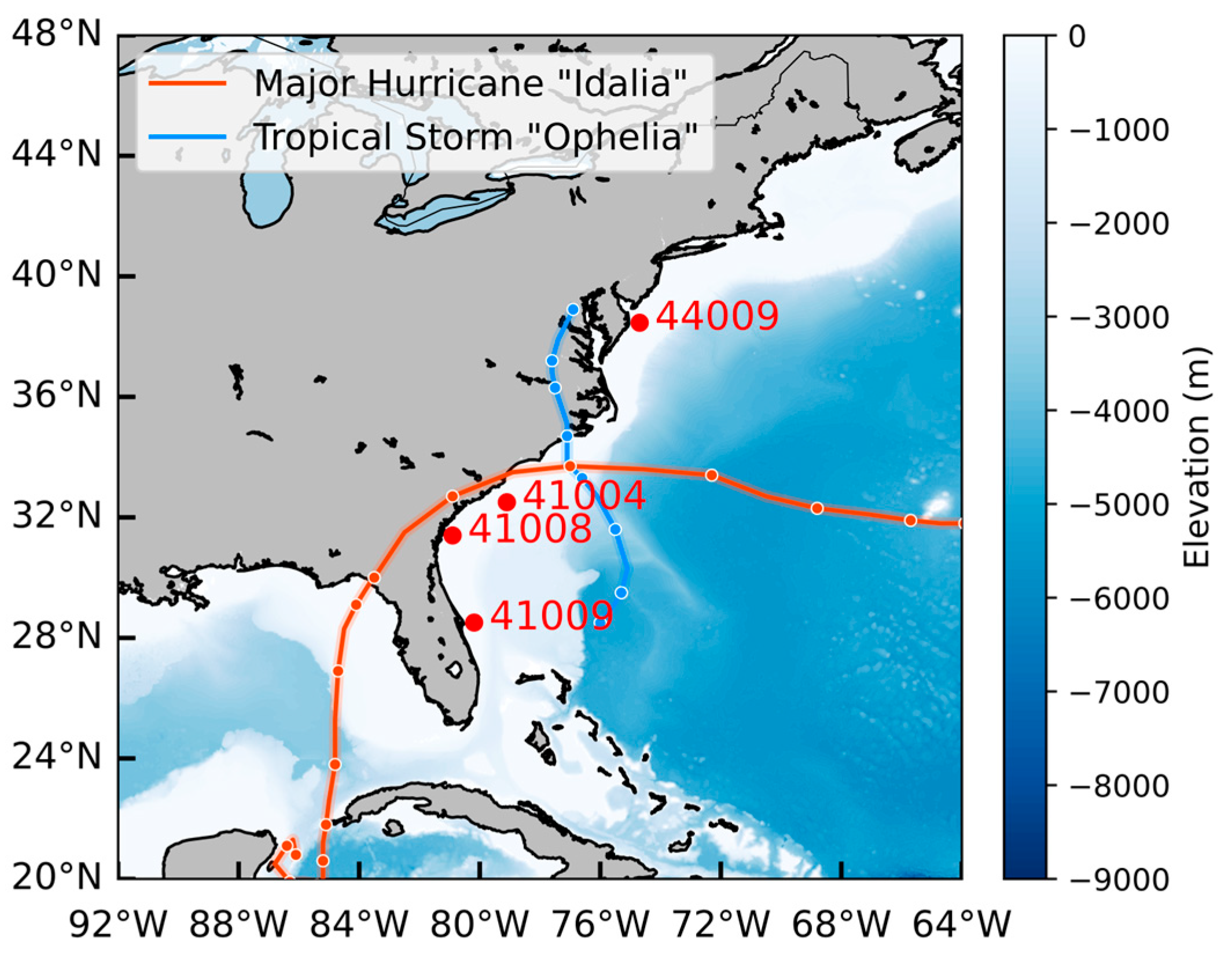
As shown in Figure 1, the four buoys used in this study are located in the North Atlantic, adjacent to the U.S. East Coast, with their detailed geographic locations and water depth parameters listed in

Table 2. The detailed locations and water depth parameters of the selected buoys.

Buoy ID	Latitude (° N)	Longitude (° W)	Depth (m)
44009	38.460	74.692	24
41004	32.502	79.099	35
41008	31.400	80.866	16
41009	28.508	80.185	24

. All four buoys are distributed along a north–south axis, covering a large geographical span. This distribution enables them to capture the oceanic environmental characteristics across different latitudinal regions. Compared with other buoys in the same region, these buoys provide more complete data records with fewer missing values. In addition, they are located in areas with frequent tropical cyclone activity, offering strong capability for monitoring extreme weather events and capturing the impacts of hurricanes and tropical storms on the nearshore marine environment. During such events, strong winds and pressure variations significantly influence the marine environment, leading to a noticeable increase in WVHT. In summary, these four buoy stations serve as ideal observation sites for studying WVHT prediction.

2.2. Data Overview

The data used in this study have a high temporal resolution, with a time interval of 1 h. During preprocessing, missing values in the original observational data were filled using the forward-fill method to ensure the continuity and completeness of the time series. To build and evaluate the predictive performance of the model, the dataset was divided into training, validation, and test sets in a 7:1:2 ratio, strictly following the chronological order.

Table 3. The statistical information of the buoy datasets.

Buoy ID	Date (Day Month Year HH:MM)	Data Volume	WVHT Range (m)
44009	01 July 2021 22:40–31 December 2023 23:40	21,914	[0.25, 6.03]
41004	10 July 2021 04:40–31 December 2023 23:40	21,716	[0.27, 8.29]
41008	01 January 2019 00:50–16 June 2023 09:50	39,058	[0.11, 4.54]
41009	01 January 2019 00:40–31 December 2023 23:40	43,824	[0.02, 9.74]

summarizes the statistical characteristics of the processed WVHT data from the selected buoy stations. The data from the four stations used in this study span from approximately two and a half to five years, covering multiple observation periods from 2019 to 2023. Specifically, the records from Stations 44009 and 41004 cover about two and a half years, those from Station 41008 about four and a half years, and those from Station 41009 extend to five years. The selection of these time periods is based on the following considerations. First, the selected periods contain minimal missing data and are of high quality. Second, time series of different lengths facilitate the evaluation of model performance across datasets with varying durations. In addition, the selected periods include multiple typical extreme weather events, providing reliable samples for assessing the model’s wave prediction capability under complex meteorological conditions.

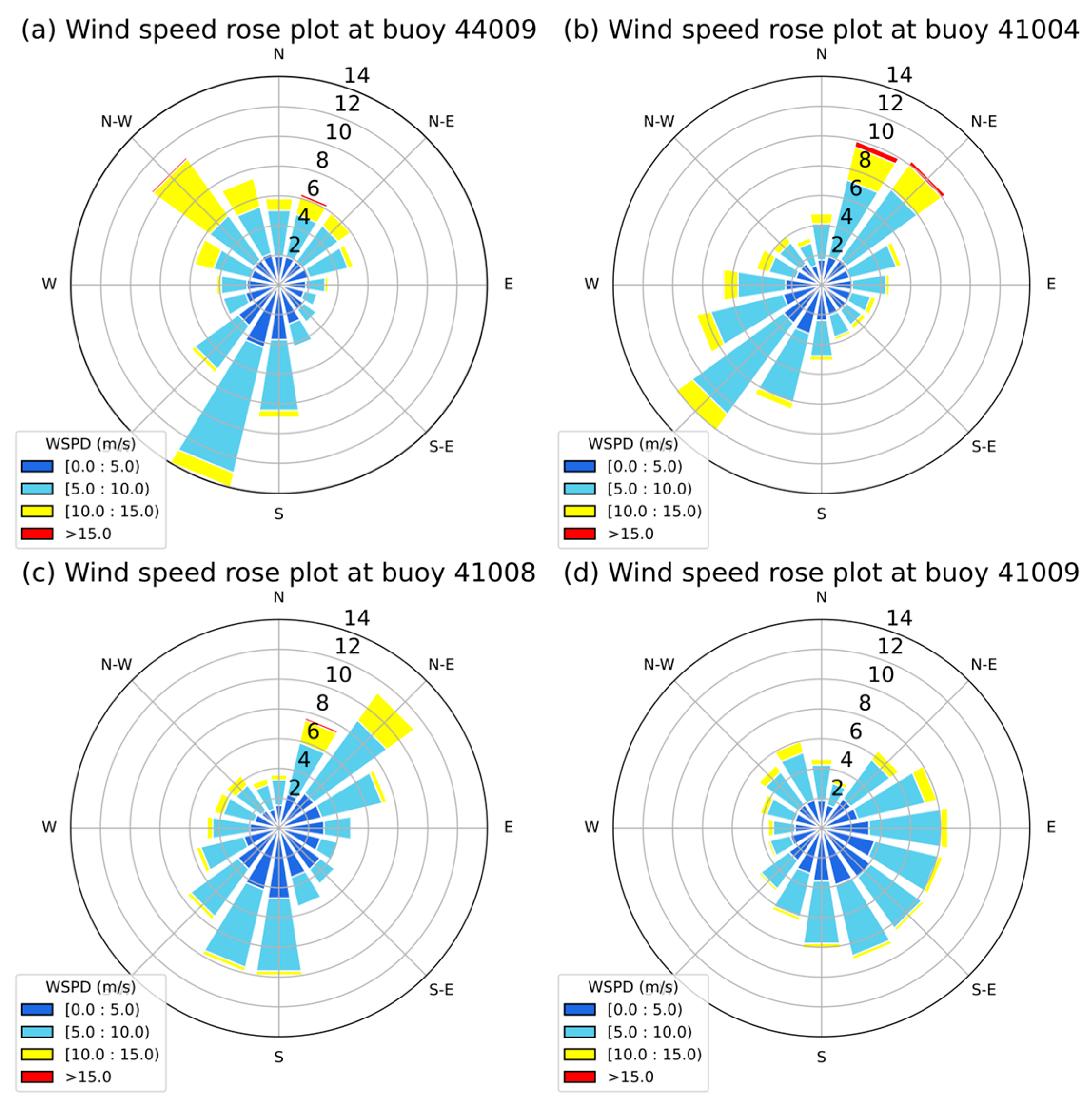
To intuitively display the WSPD and WDIR characteristics at each buoy station, this paper presents the rose diagrams shown in Figure 2. A rose diagram is a commonly used visualization tool for directional data that clearly illustrates the frequency distribution from different directions. In the figure, WSPD values are divided into four levels: 0–5 m/s, 5–10 m/s, 10–15 m/s, and >15 m/s. Different colors represent different WSPD intervals, and the radius of each sector corresponds to the frequency of occurrence from a specific direction—the longer the radius, the higher the frequency. From Figure 2, it can be seen that the dominant WDIR at Station 44009 is northwest and south-southwest, originating from the two landward sides adjacent to the buoy location. The maximum frequency of winds from the northwest is about 10%, while that of winds from the south-southwest is about 14%. Stronger winds of 10–15 m/s mainly come from the northwest, with overall WSPD mostly concentrated in the 5–10 m/s range. At Station 41004, WDIRs are mainly concentrated in the north-northeast and southwest directions, roughly parallel to the coastal terrain. The maximum frequency of winds from the southwest is about 12%, and that of winds from the northeast is about 10%. Winds stronger than 15 m/s mainly originate from the northeast. At Station 41008, WDIRs are primarily from the south-southwest and northeast, with the maximum frequency of winds from the northeast, around 11% and that of winds from the south, about 10%, consistent with the nearby coastline orientation. At Station 41009, winds mainly originate from the southeast, south, and east, with WSPD mostly in the 5–10 m/s range. Overall, there are significant differences in WSPD and WDIR distributions among the stations. This spatial heterogeneity poses challenges for deep learning models.

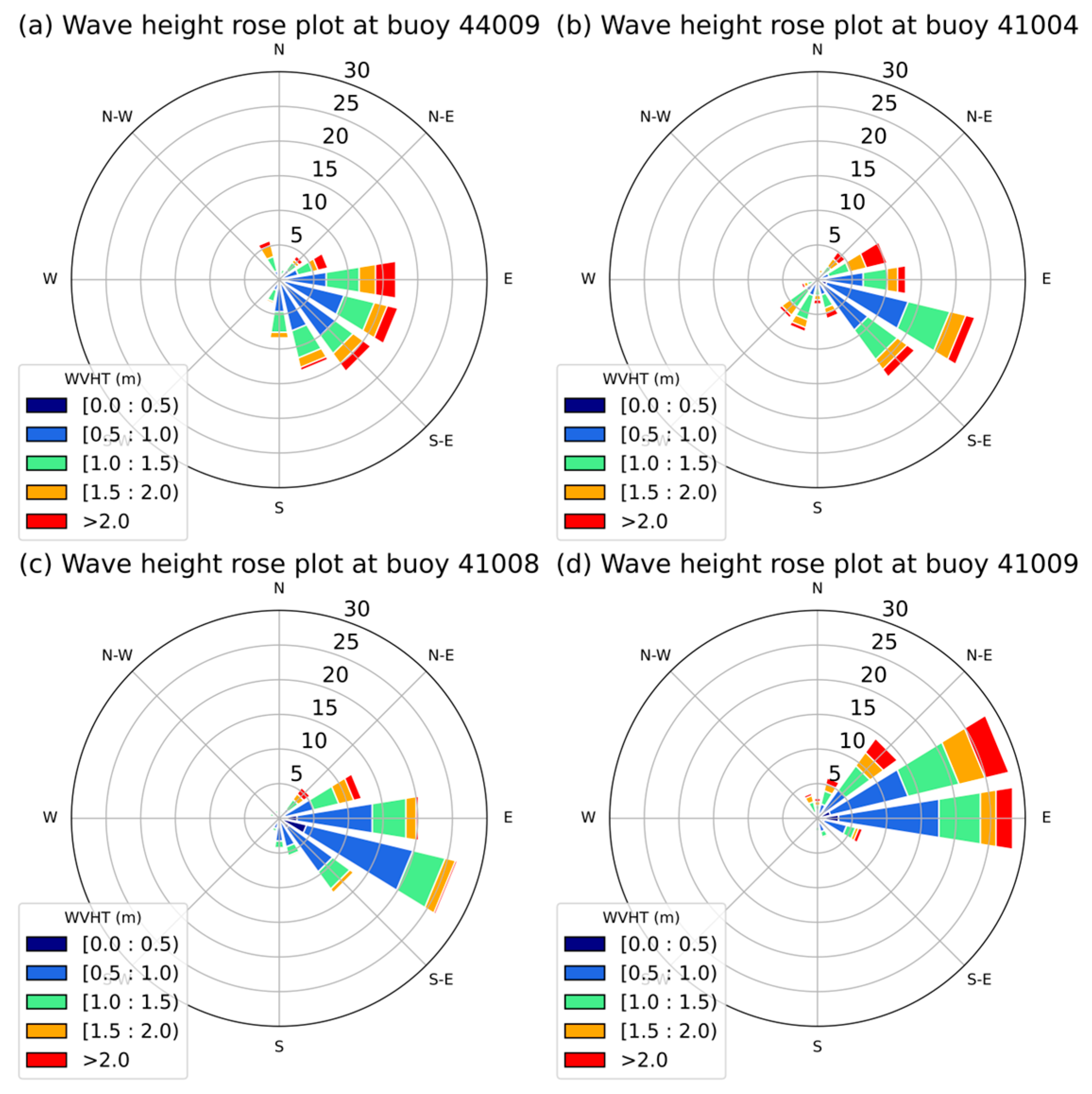
To intuitively display the characteristics of WVHT at each buoy station, Figure 3 presents rose diagrams of WVHT based on the MWD. The WVHT is divided into five intervals: 0–0.5 m, 0.5–1.0 m, 1.0–1.5 m, 1.5–2.0 m, and >2.0 m. Different colors correspond to different wave height intervals, and the radius of each colored sector represents the frequency of waves coming from that direction. At buoy 44009, waves mainly come from the east to east-southeast direction, with the highest frequency of around 17% from due east, about 16% from east-southeast by east, and approximately 15% from southeast. Waves exceeding 2.0 m in height mainly occur from the due east direction. At buoy 41004, waves predominantly come from east-southeast by east, with the highest frequency of about 23% from east-southeast by east and around 12% from southeast. Overall, wave heights are mostly concentrated in the 0.5–1.5 m range, with waves over 2.0 m distributed in the southeast and northeast directions. At buoy 41008, waves mainly come from east to east-southeast, with a maximum frequency of about 26%, and occasional strong waves over 2.0 m are recorded from the northeast direction. At buoy 41009, waves primarily come from east to east-northeast, with frequencies of approximately 27% from due east and 28% from east-northeast, and about 10% of waves exceeding 2.0 m in height.

2.3. Data Correlation and Feature Selection

To minimize computational redundancy while utilizing as many feature variables as possible, this study employs the Pearson correlation coefficient (r) to select model input features. The Pearson correlation coefficient is a statistical measure that quantifies the linear relationship between two variables, and its calculation is defined as follows:

$$\mathit{r} = {\displaystyle \frac{{\sum }_{\mathit{i}=1}^{\mathit{n}}({\mathit{x}}_{\mathit{i}}-\overline{\mathit{x}})({\mathit{y}}_{\mathit{i}}-\overline{\mathit{y}})}{\sqrt{{\sum }_{\mathit{i}=1}^{\mathit{n}}{({\mathit{x}}_{\mathit{i}}-\overline{\mathit{x}})}^2{\sum }_{\mathit{i}=1}^{\mathit{n}}{({\mathit{y}}_{\mathit{i}}-\overline{\mathit{y}})}^2}}}$$

(1)

where n is the sample size; ${\mathit{x}}_{\mathit{i}}$ and $y_i$ represent the i-th paired sample; $\overline{\mathit{x}}={\displaystyle \frac{1}{\mathit{n}}}{\displaystyle {\sum }_{\mathit{i}=1}^{\mathit{n}}}{\mathit{x}}_{\mathit{i}}$ and $\overline{\mathit{y}}={\displaystyle \frac{1}{\mathit{n}}}{\displaystyle {\sum }_{\mathit{i}=1}^{\mathit{n}}}{\mathit{y}}_{\mathit{i}}$ denote the mean values of x and y, respectively. When r = 1, it indicates a perfect positive linear correlation between the two variables; when r = −1, it indicates a perfect negative linear correlation; and when r = 0, it indicates no linear correlation between the two variables.

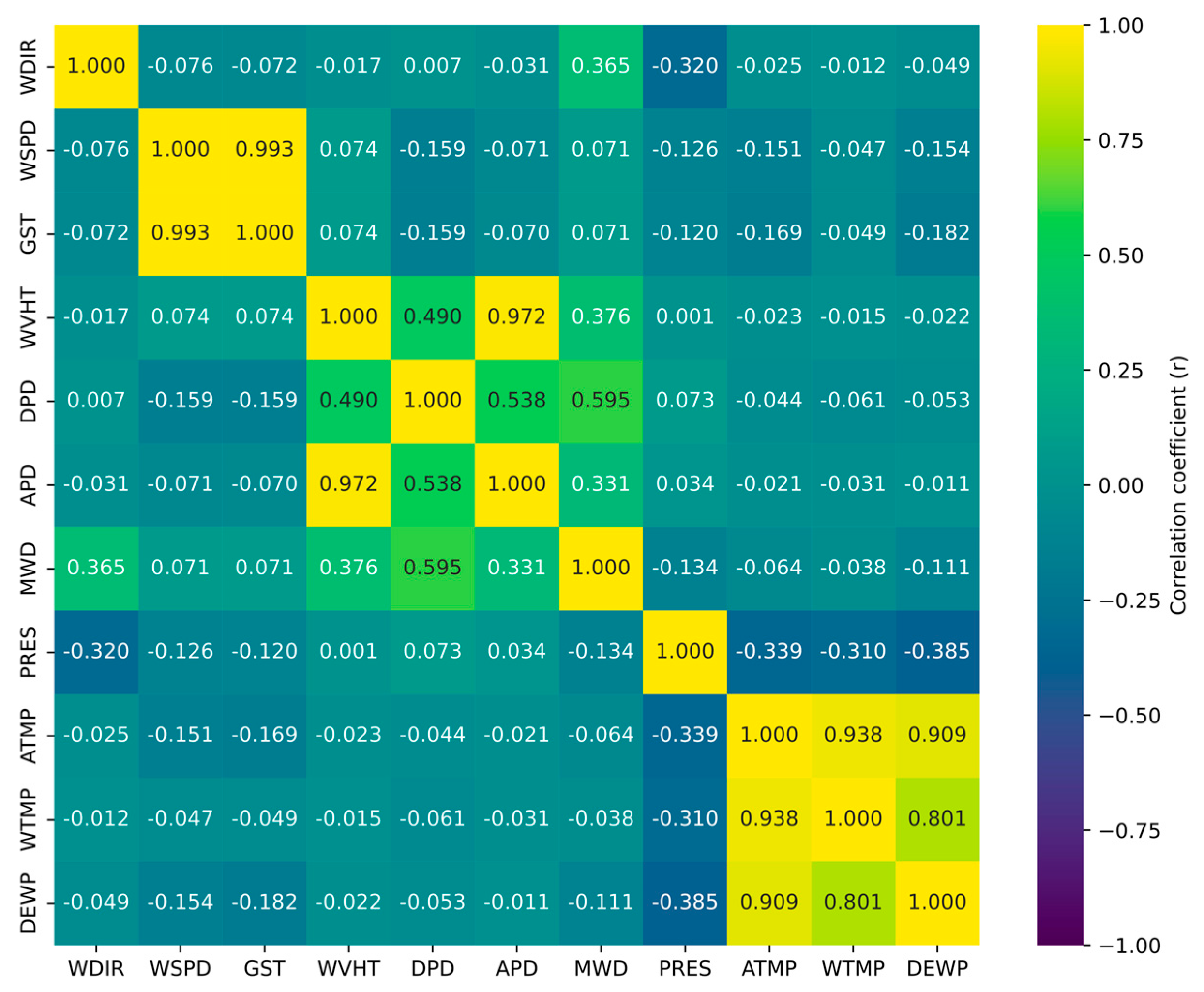
This study calculates the Pearson correlation coefficients among environmental variables at buoy 41008. Figure 4 presents the corresponding correlation coefficient matrix. Among the wind speed–related variables, the correlation coefficient between GST and WSPD is as high as 0.993, indicating an almost perfect linear correlation and substantial information redundancy. Considering that WSPD is more widely used in coastal environmental modeling and wave forecasting and has clearer physical interpretability, only WSPD is retained as the wind speed–related input feature. Among the wave period–related variables, the correlation coefficient between DPD and APD is 0.538, indicating a moderate correlation and partial information redundancy. Given that APD is more robust to high-frequency noise and better reflects the overall characteristics of wave energy distribution, APD is retained while DPD is excluded. Among the temperature-related and humidity-related variables, the correlation coefficients between ATMP and DEWP and between ATMP and WTMP are 0.938 and 0.801, respectively, indicating strong linear correlations. Meanwhile, ATMP and DEWP contain a considerable number of missing values in the observational data. Considering both information redundancy and data completeness, only WTMP is retained as the temperature-related input feature. Based on the above analysis, a total of seven variables are selected as model input features: WSPD, WDIR, WVHT, APD, MWD, PRES, and WTMP.

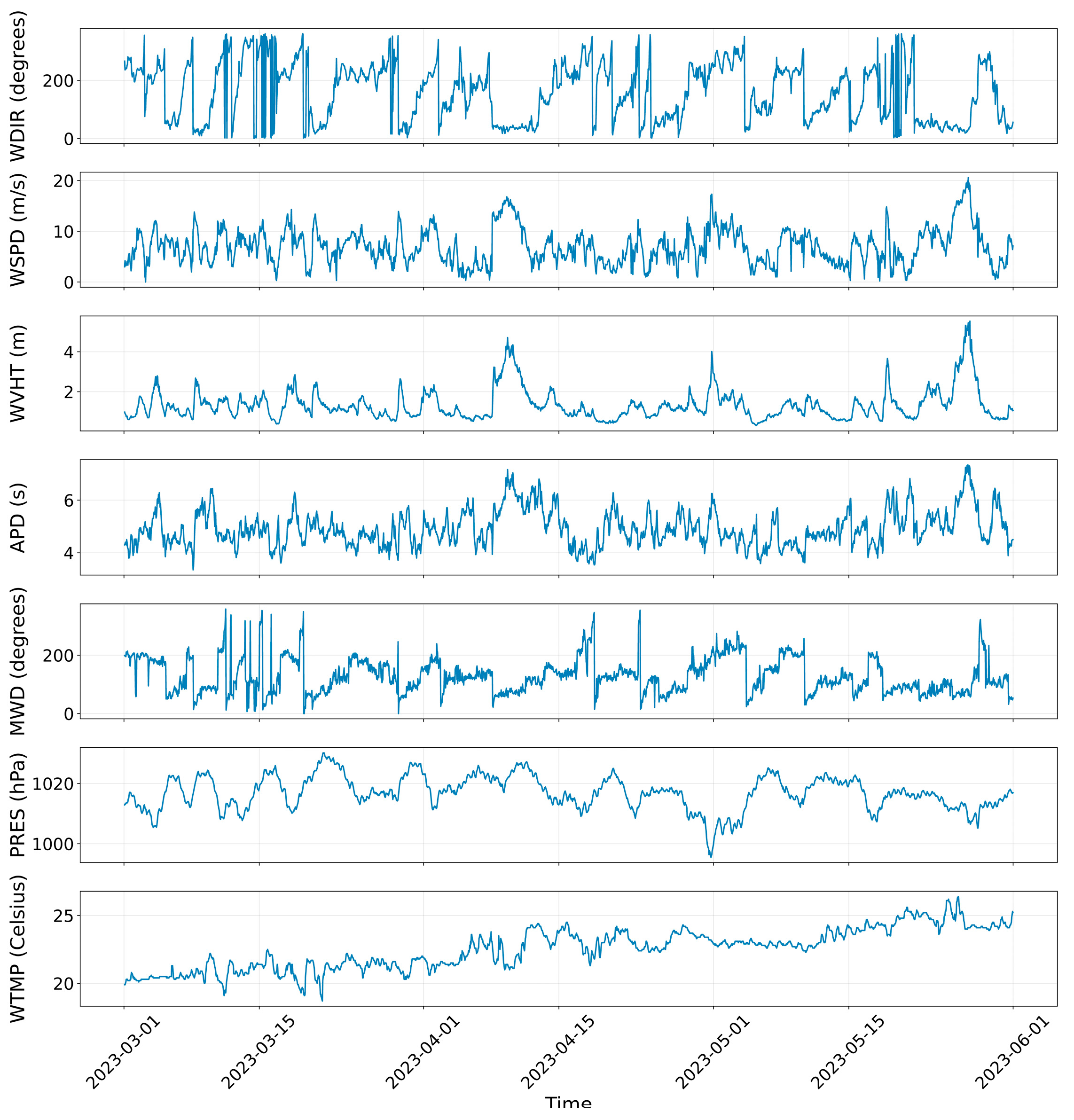
Figure 5 presents the time series profiles of seven input features derived from buoy 41004 between 1 March–June 2023. All variables exhibit pronounced nonstationarity and complex temporal dynamics. Significant differences exist in their value ranges and physical characteristics: PRES varies narrowly around 1000–1020 hPa, whereas WVHT fluctuates within 0–5 m, and WDIR shows cyclic behavior within 0–360°, leading to artificial discontinuities. In addition, the variables differ markedly in temporal variability. WTMP evolves smoothly, while WDIR and MWD may change abruptly over short periods. Wave-related variables such as WVHT and APD display strong randomness and intermittency, often influenced by storms and atmospheric conditions. Furthermore, inter-variable relationships are time-dependent. WSPD is generally positively correlated with WVHT, though this relationship may weaken or lag under extreme conditions. PRES is closely coupled with wind-wave dynamics, while WTMP varies more gradually and mainly reflects long-term effects. These characteristics highlight the challenges of modeling multi-scale and nonlinear ocean processes.

3. Methods

3.1. CEEMDAN

CEEMDAN serves as a signal decomposition approach for handling nonlinear and non-stationary time series. Through CEEMDAN decomposition, the original sequence is ultimately broken down into a set of intrinsic mode functions (IMFs) and a residual signal. Let us define the operator ${\mathrm{E}\mathrm{M}\mathrm{D}}_{\mathrm{k}}\left(·\right)$ which, given a signal, produces the k-th mode obtained by EMD. In EMD, each IMF must satisfy two conditions: (1) The number of local maxima and local minima of the IMF must be equal to the number of zero-crossings or differ by at most one. (2) At any moment, the mean of the upper and lower envelopes of the IMF should be zero at each point, meaning that the upper and lower envelopes are locally symmetric with respect to the time axis. Let ${\mathrm{w}}_{\mathrm{i}}\left(\mathrm{t}\right)$ be white noise with $\mathrm{N}\left(\mathrm{0,1}\right)$. If $\mathrm{x}\left(\mathrm{t}\right)$ is the original signal, we can describe the CEEMDAN algorithm in detail using the following steps:

• Initialization and addition of noise

For the given original time series, add Gaussian white noise to obtain multiple noise-added signals:

$$x_i\left(t\right)=x\left(t\right)+ϵw_i\left(t\right), i=1, 2,\dots , N$$

(2)

where $ϵ$ is the noise amplitude, and $N$ is the total number of noise-assisted signals.

2.

Decomposition of the first IMF

Apply EMD to each noisy signal to obtain the corresponding first-order IMF:

$${\mathrm{I}\mathrm{M}\mathrm{F}}_{1,i}\left(t\right)={\mathrm{E}\mathrm{M}\mathrm{D}}_1\left(x_i\left(t\right)\right), i=1, 2,\dots , N$$

(3)

Calculate the average of all the first-order IMFs to represent the first IMF of the original signal:

$${\mathrm{I}\mathrm{M}\mathrm{F}}_1\left(t\right)={\displaystyle \frac{1}{N}}{\sum }_{i=1}^N{\mathrm{I}\mathrm{M}\mathrm{F}}_{1,i}\left(t\right)$$

(4)

3.

Calculation of the residual and addition of noise

Subtract the first IMF from the original signal to obtain the residual signal:

$$r_1\left(t\right)=x\left(t\right)-{\mathrm{I}\mathrm{M}\mathrm{F}}_1\left(t\right)$$

(5)

Add Gaussian white noise again to the residual signal to obtain a new noise-added signal:

$$r_{1,i}\left(t\right)=r_1\left(t\right)+ϵw_i\left(t\right), i=1, 2,\dots , N$$

(6)

4.

Decomposition of subsequent IMFs

Perform EMD on each new noise-added signal to obtain the corresponding second-order IMF:

$${\mathrm{I}\mathrm{M}\mathrm{F}}_{2,i}\left(t\right)={\mathrm{E}\mathrm{M}\mathrm{D}}_2\left(r_{1,i}\left(t\right)\right), i=1, 2,\dots , N$$

(7)

Similarly, take the mean as the second-order IMF of the original signal:

$${\mathrm{I}\mathrm{M}\mathrm{F}}_2\left(t\right)={\displaystyle \frac{1}{N}}{\sum }_{i=1}^N{\mathrm{I}\mathrm{M}\mathrm{F}}_{2,i}\left(t\right)$$

(8)

5.

Repeat Steps 3 and 4

Repeat the above steps until the residual signal satisfies a stopping criterion (e.g., the residual signal is sufficiently small or contains only one maximum and minimum). For k = 2, …, K calculate the k-th residue:

$$r_k\left(t\right)=r_{k-1}\left(t\right)-{\mathrm{I}\mathrm{M}\mathrm{F}}_k\left(t\right)$$

(9)

The final residual is:

$$R\left(t\right)=x\left(t\right)-{\sum }_{k=1}^K{\mathrm{I}\mathrm{M}\mathrm{F}}_k\left(t\right)$$

(10)

6.

Final output

Finally, the provided signal $x\left(t\right)$ is formulated as:

$$x\left(t\right)={\sum }_{k=1}^K{\mathrm{I}\mathrm{M}\mathrm{F}}_k\left(t\right)+R\left(t\right)$$

(11)

3.2. iTransformer

3.2.1. Token Construction for Multivariate Time Series Data

In multivariate time series, each variable typically represents a set of independently recorded observation sequences, each reflecting the dynamic changes in a particular dimension within the system. For example, in health monitoring scenarios, common variables include heart rate, blood pressure, and body temperature, each corresponding to the changing trajectories of different physiological states of the human body; in macroeconomic analysis, key indicators such as unemployment rate, sales volume, and exchange rate may be involved, each depicting the economic conditions from different perspectives. Although these variables may share similar trends to some extent or be influenced by common factors, they inherently possess different semantic characteristics. Their measurement units, scale ranges, and statistical distributions usually differ significantly. This heterogeneity poses greater challenges for multivariate time series modeling, especially in modeling relationships between variables and feature representation. However, many traditional time series forecasting models often assume that variables have the same statistical properties, neglecting the impact of differences between variables, which may limit the models’ ability to capture complex real-world scenarios and reduce prediction accuracy.

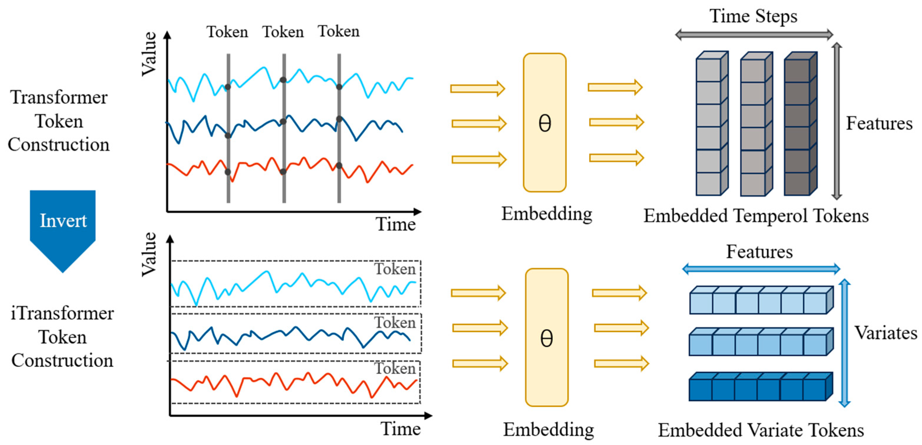
Unlike natural language, which has an inherent word-segmentation mechanism, the basic modeling unit in time series prediction models based on the Transformer architecture is called a Token. As shown in the upper half of Figure 6, traditional methods typically represent the set of all variables at a given time point as a single temporal Token and generate the corresponding embedded temporal Token through the model’s Embedding layer. Horizontally, these Embedded Temporal Tokens reflect data information from different time points; vertically, each Embedded Temporal Token contains the features of all variables at that specific time point. However, due to limited receptive fields and the failure to account for potential lag relationships between variables, this data input structure struggles to fully capture rich semantic information and may even introduce noise, thereby limiting the attention mechanism’s ability to model relationships between Tokens. Furthermore, when different variables at the same time point are mapped to a single Token, the originally independent variable features are blended into multidimensional features, making it difficult for the model to distinguish between variables and preventing it from clearly capturing the associations among them.

In contrast, as shown in the lower half of Figure 6, iTransformer employs an inverted modeling strategy to process multivariate time series. It independently constructs a complete time series of each variable into a variate Token and generates a corresponding Embedded Variate Token through an Embedding layer. Horizontally, each Embedded Variate Token reflects the features of that variable across all time points; vertically, different Embedded Variate Tokens represent the independent information of different variables. Through this variable-centric modeling approach, the attention mechanism can more naturally uncover correlations among multiple variables, making it particularly suitable for multidimensional time series data with a large number of variables and complex interdependencies. Furthermore, the synergy between iTransformer’s feedforward network and layer normalization mechanism effectively mitigates the impact of differences in measurement units and scales across variables, thereby learning sequence features better suited for time series forecasting.

3.2.2. iTransformer Model Architecture

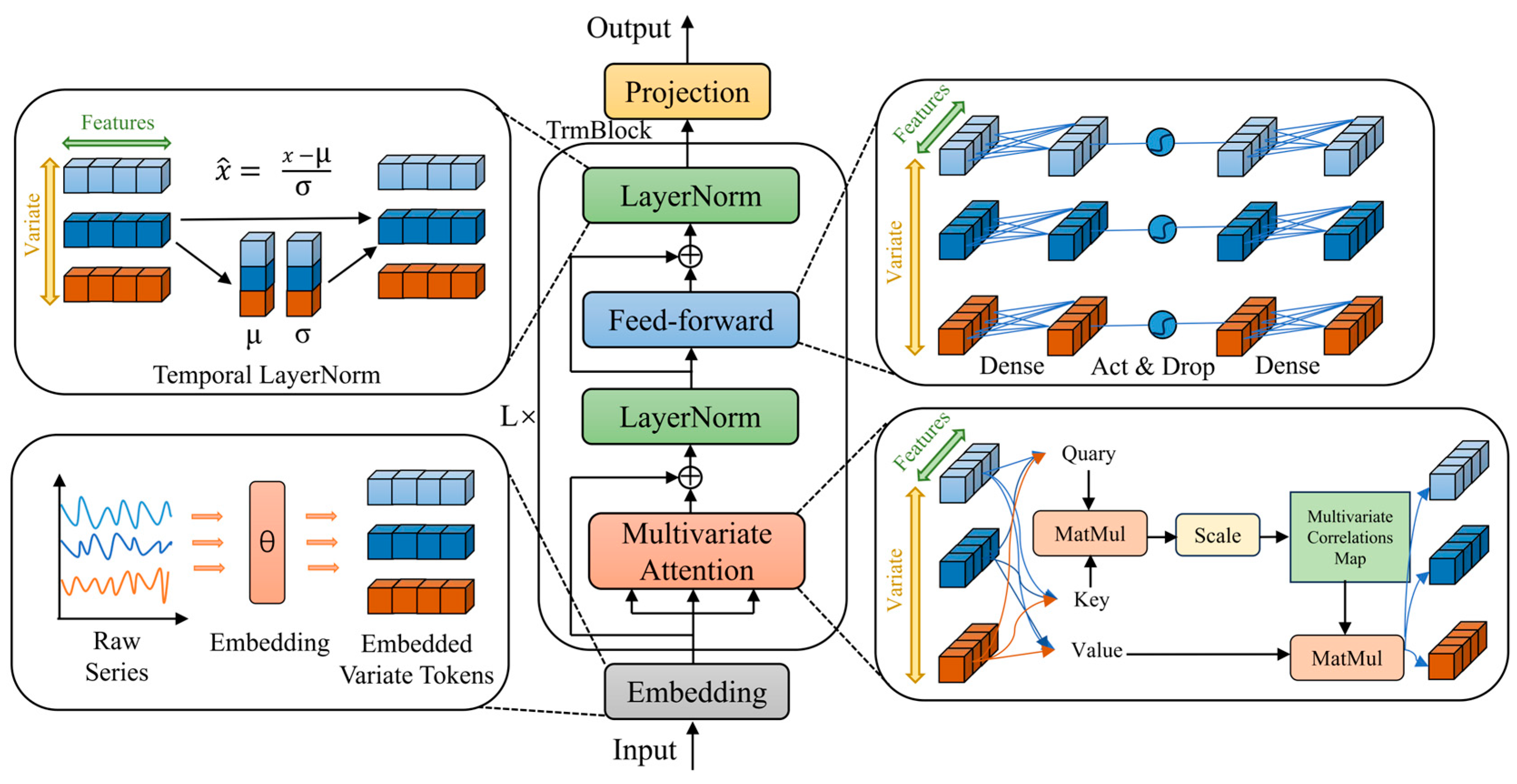
As illustrated in Figure 7, iTransformer is built upon an encoder-only framework, which consists of an embedding layer (Embedding), a projection layer (Projection), and multiple Transformer modules (TrmBlock). These components can be stacked to effectively model multivariate time series data.

Given a multidimensional time series $\mathbf{X}\in {\mathbb{R}}^{T\times N}$ with a time span of T and N variables, we denote ${\mathbf{X}}_{t,:}$ as the set of all variables at a given time step, and ${\mathbf{X}}_{:,n}$ as the complete sequence of a single variable. As mentioned earlier, compared to ${\mathbf{X}}_{t,:}$, ${\mathbf{X}}_{:,n}$ possesses consistent semantics and units of measurement. Unlike previous models that treat ${\mathbf{X}}_{t,:}$ as independent tokens, iTransformer employs an embedding layer to learn the series representation of ${\mathbf{X}}_{:,n}$ and independently aggregates the global features of each variable, resulting in:

$$\mathbf{H}=\left\{{\mathbf{h}}_1, {\mathbf{h}}_2,\dots , {\mathbf{h}}_N\right\}\in {\mathbb{R}}^{N\times D}$$

(12)

In particular, ${\mathbf{h}}_i\in {\mathbb{R}}^D$ encapsulates the complete temporal variation information of the corresponding variable over past time periods, thereby forming a Variate Token for each variable. In subsequent layers, information is exchanged between Variate Tokens via an auto-attention mechanism; within each Variate Token, layer normalization unifies the measurement units and feature distributions across different variables, while a fully connected feedforward network performs feature encoding. Finally, the mapping layer maps each Variate Token to a prediction result. The entire computational process is represented as follows:

$${\mathbf{h}}_n^0=\mathrm{E}\mathrm{m}\mathrm{b}\mathrm{e}\mathrm{d}\mathrm{d}\mathrm{i}\mathrm{n}\mathrm{g}\left({\mathbf{X}}_{:,n}\right)$$

(13)

$${\mathrm{H}}^{\mathrm{l}+1}=\mathrm{T}\mathrm{r}\mathrm{m}\mathrm{B}\mathrm{l}\mathrm{o}\mathrm{c}\mathrm{k}\left({\mathrm{H}}^{\mathrm{l}}\right)$$

(14)

$${\widehat{\mathbf{Y}}}_{:,n}=\mathrm{P}\mathrm{r}\mathrm{o}\mathrm{j}\mathrm{e}\mathrm{c}\mathrm{t}\mathrm{i}\mathrm{o}\mathrm{n}\left({\mathbf{h}}_n^L\right)$$

(15)

Both the embedding layer and the mapping layer are implemented using a Multilayer Perceptron (MLP). Since the temporal order between time steps is already implicit in the arrangement of the neurons, the model can perceive the sequential relationships between time steps, thereby eliminating the need for additional position embedding.

3.3. CEEMDAN-iTransformer Model Design and Implementation

WVHT is governed by the strong coupling of atmospheric forcing and ocean dynamics, including wind fields, pressure gradients, and air–sea interactions. As a result, the WVHT time series exhibits pronounced nonlinearity and nonstationarity, characterized by both gradual background evolution and abrupt fluctuations induced by extreme weather events such as storms. From a temporal perspective, the series contains multi-scale components, including high-frequency variations at the hourly scale driven by local wind changes, as well as low-frequency trends at daily to seasonal scales associated with large-scale atmospheric circulation. In addition, observational data are often contaminated by measurement noise and environmental disturbances. These complexities make it difficult for conventional linear or single-scale models to capture both short-term variability and long-term trends. Therefore, CEEMDAN is employed to decompose the original WVHT series into multi-scale components for improved feature extraction.

Figure 8 illustrates the original WVHT time series at buoy 41009 and its decomposition using CEEMDAN. The original series is decomposed into multiple IMFs and a residual, exhibiting clear multi-scale characteristics with decreasing frequency and amplitude. The high-frequency components (IMF1–IMF6) mainly capture rapid and irregular fluctuations, reflecting short-term wave variability driven by wind disturbances. The intermediate components (IMF7–IMF10) represent relatively stable oscillations associated with medium-scale wave evolution. The low-frequency components (IMF11–IMF15) show long-period variations, characterizing the long-term behavior of WVHT. The residual term varies smoothly and represents the overall trend of the series. Most IMFs exhibit approximately zero-mean oscillations, indicating that CEEMDAN effectively alleviates mode mixing and enhances physical interpretability. These results demonstrate the pronounced multi-scale nature of WVHT. Direct modeling of the raw series may increase complexity and reduce predictive accuracy. Therefore, a “decomposition–prediction–reconstruction” framework is adopted to model each component separately and improve forecasting performance.

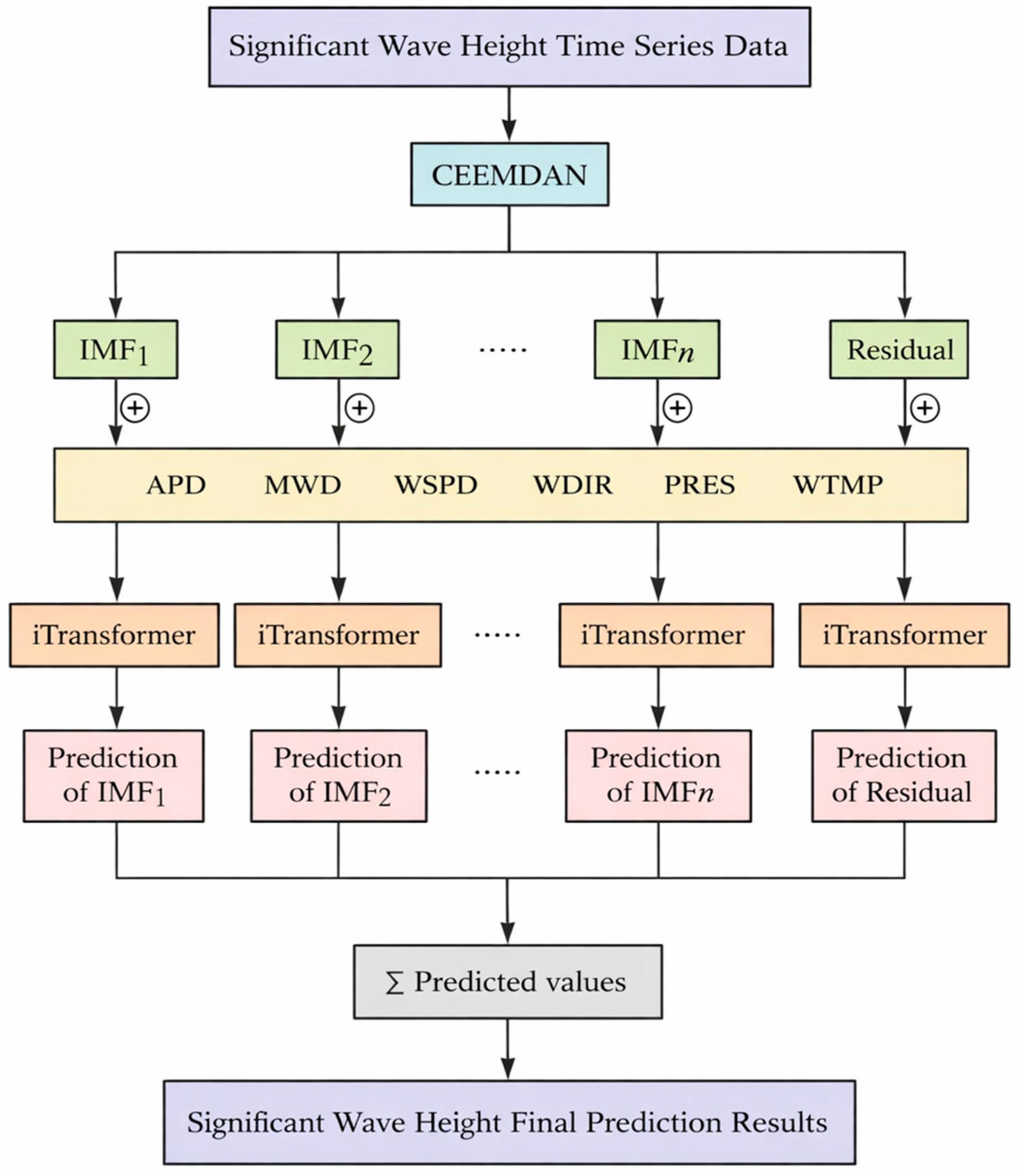
On this basis, a hybrid model integrating CEEMDAN and iTransformer is developed for WVHT forecasting. The overall framework, illustrated in Figure 9, can be divided into four stages.

(1)

Signal decomposition: The original WVHT time series is first decomposed using CEEMDAN into multiple IMFs with different scale characteristics and a residual component, transforming the complex nonstationary signal into several relatively stationary sub-series.

(2)

Input feature construction: For each IMF component, a multivariate input feature set is constructed by incorporating six key environmental variables, including WDIR, WSPD, MWD, PRES, WTMP, and APD, to fully capture the coupling relationships and complementary information between WVHT and external environmental factors.

(3)

Component-wise modeling and prediction: Independent iTransformer models are trained for each IMF and the residual component, enabling targeted modeling of fluctuations at different scales and enhancing the ability to capture complex nonlinear relationships and long-term dependencies.

(4)

Result reconstruction: The predicted results of all IMFs and the residual are aggregated point by point in chronological order to reconstruct the final WVHT prediction.

Through this “decomposition-modeling-reconstruction” framework, the proposed CEEMDAN-iTransformer model effectively exploits multi-scale structural features of WVHT while mitigating the limitations of single models in handling noisy and nonstationary data, thereby improving prediction accuracy, stability, and generalization ability.

Figure 9. CEEMDAN-iTransformer model prediction process.

Figure 9. CEEMDAN-iTransformer model prediction process.

4. Results and Discussion

4.1. Experimental Setup

4.1.1. Evaluation Metrics

To comprehensively evaluate the predictive performance of the CEEMDAN-iTransformer model for WVHT, this paper employs four commonly used evaluation metrics to conduct a quantitative analysis of the model’s predictions: Mean Absolute Error (MAE), Root Mean Square Error (RMSE), Mean Absolute Percentage Error (MAPE), and Correlation Coefficient (CC). The calculation formulas are as follows:

$$\mathrm{M}\mathrm{A}\mathrm{E}={\displaystyle \frac{1}{n}}{\sum }_{i=1}^n\left|{\widehat{y}}_i-y_i\right|$$

(16)

$$\mathrm{R}\mathrm{M}\mathrm{S}\mathrm{E}=\sqrt{{\displaystyle \frac{1}{n}}{\sum }_{i=1}^n{\left({\widehat{y}}_i-y_i\right)}^2}$$

(17)

$$\mathrm{M}\mathrm{A}\mathrm{P}\mathrm{E}={\displaystyle \frac{1}{n}}{\sum }_{i=1}^n\left|{\displaystyle \frac{{\widehat{y}}_i-y_i}{y_i}}\right|\times 100\%$$

(18)

$$\mathrm{C}\mathrm{C}={\displaystyle \frac{{\sum }_{i=1}^n({\widehat{y}}_i-\overline{\widehat{y}})(y_i-\overline{y})}{\sqrt{{\sum }_{i=1}^n{({\widehat{y}}_i-\overline{\widehat{y}})}^2}\sqrt{{\sum }_{i=1}^n{(y_i-\overline{y})}^2}}}$$

(19)

where n represents the total number of samples; $y_i$ represents the observed value of WVHT at time step i; ${\widehat{y}}_i$ denotes the model’s predicted value; $\overline{y}$ enotes the mean of the observed values; and $\overline{\widehat{y}}$ denotes the mean of the predicted values. Smaller values of MAE, RMSE, and MAPE, along with CC value closer to 1, indicate lower prediction errors and better model performance.

4.1.2. Parameter Settings

This study selects four advanced time series forecasting models for comparison in the experiment: iTransformer, TimesNet [38], Crossformer [39], and DLinear [40]. In order to reduce the influence of varying parameter configurations on model effectiveness, appropriate parameter settings have been applied to all five models. The key settings include using ReLU as the activation function, Adam as the optimizer, a learning rate of 0.0001, a dropout rate of 0.1, and a batch size of 32.

The goal of this study is to develop an accurate WVHT prediction model capable of forecasting WVHT in coastal areas prone to hurricanes or tropical storms. Setting a reasonable prediction time length is crucial to achieve this goal. Based on previous research, this study utilizes data from the past 24 h to predict WVHT for the next 3 h, 6 h, 12 h, 24 h, and 48 h.

4.2. Total Prediction Performance Evaluation

4.2.1. Prediction Results of Buoy 41009

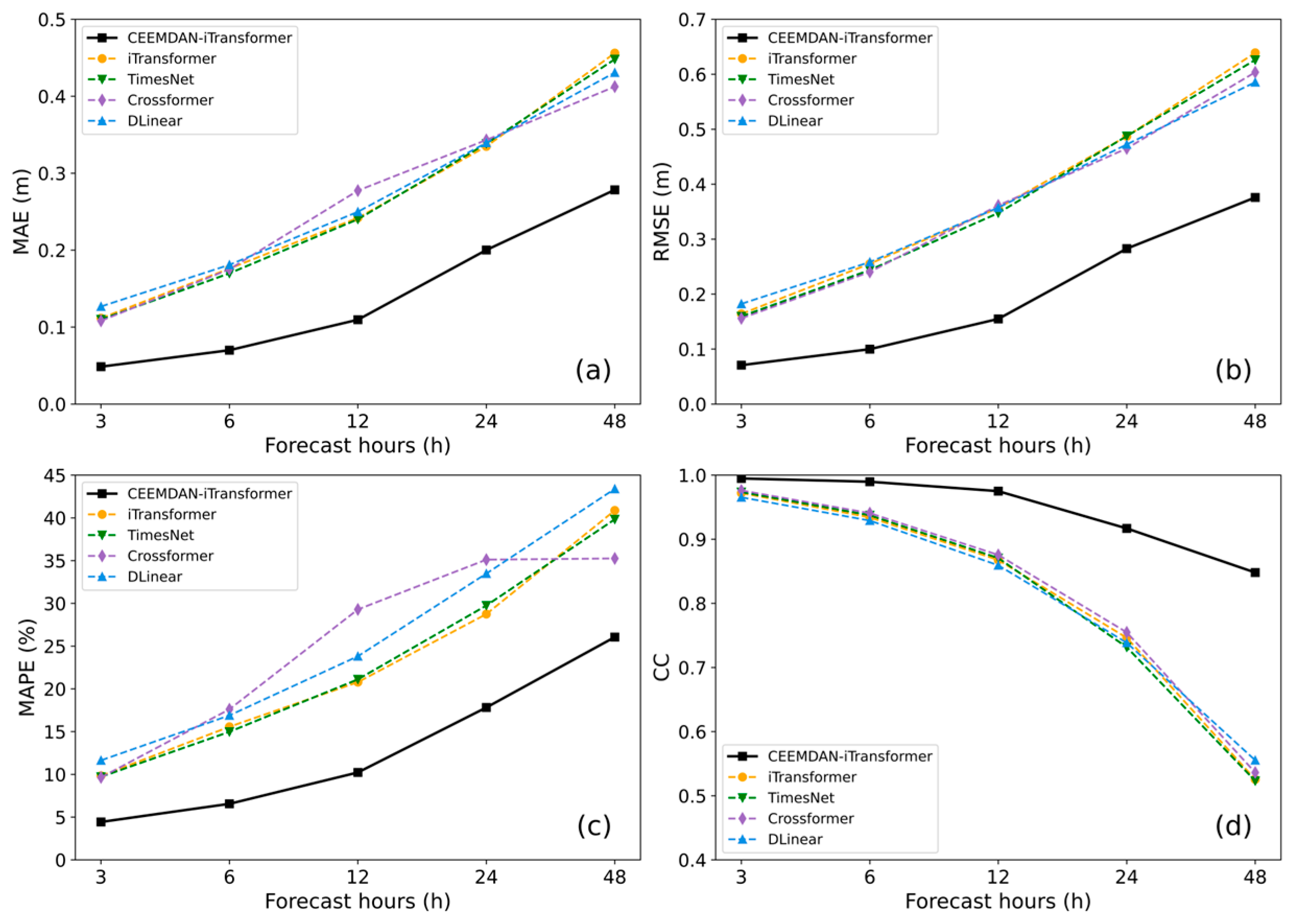
This section systematically evaluates the WVHT prediction performance of the CEEMDAN-iTransformer, iTransformer, TimesNet, Crossformer, and DLinear models across five different forecast horizons.

Table 4. Comparison of errors from various models at buoy 41009 for different forecast durations.

Forecast Hours	Metrics	CEEMDAN-iTransformer	iTransformer	TimesNet	Crossformer	DLinear
3 h	MAE (m) ↓	0.0486	0.1116	0.1100	0.1082	0.1268
	RMSE (m) ↓	0.0708	0.1641	0.1596	0.1560	0.1823
	MAPE (%) ↓	4.4377	9.8351	9.7153	9.6507	11.6418
	CC ↑	0.9948	0.9721	0.9735	0.9761	0.9654
6 h	MAE (m) ↓	0.0700	0.1761	0.1699	0.1752	0.1810
	RMSE (m) ↓	0.0999	0.2553	0.2439	0.2404	0.2584
	MAPE (%) ↓	6.5577	15.5664	14.9815	17.6121	16.8980
	CC ↑	0.9897	0.9341	0.9373	0.9407	0.9291
12 h	MAE (m) ↓	0.1096	0.2420	0.2402	0.2774	0.2499
	RMSE (m) ↓	0.1549	0.3568	0.3476	0.3613	0.3574
	MAPE (%) ↓	10.2268	20.7897	21.1116	29.2911	23.8160
	CC ↑	0.9750	0.8676	0.8706	0.8755	0.8594
24 h	MAE (m) ↓	0.2002	0.3348	0.3384	0.3432	0.3395
	RMSE (m) ↓	0.2828	0.4871	0.4875	0.4651	0.4724
	MAPE (%) ↓	17.8254	28.7496	29.7473	35.1132	33.4860
	CC ↑	0.9169	0.7464	0.7317	0.7548	0.7386
48 h	MAE (m) ↓	0.2784	0.4561	0.4481	0.4125	0.4308
	RMSE (m) ↓	0.3759	0.6391	0.6261	0.6037	0.5856
	MAPE (%) ↓	26.0575	40.8701	39.8318	35.2539	43.3937
	CC ↑	0.8481	0.5255	0.5232	0.5362	0.5554

“↓” indicates that a lower value of the evaluation metric corresponds to better model performance, whereas “↑” indicates that a higher value of the evaluation metric corresponds to better model performance.

presents the prediction results for buoy 41009, while Figure 10 illustrates the trends of various evaluation metrics over different forecast horizons using line charts, with different colors representing different prediction models.

As shown in Table 4, the CEEMDAN-iTransformer model demonstrates the best performance across all forecast horizons, with overall performance significantly superior to that of the other comparison models. In the 3 h, 6 h, and 12 h forecasts, the CEEMDAN-iTransformer model’s MAE increased from 0.0486 m to 0.1096 m, and its CC decreased from 0.9948 to 0.9750, reflecting the general trend of gradually accumulating errors and declining correlation as the forecast horizon increases. Compared with the other four models, the reduction in MAE ranged from 54.37% to 61.67%, while the improvement in CC ranged from 1.92% to 13.45%, indicating that this model has a significant advantage in shorter-term forecasts. When the forecast horizon was extended to 24 h and 48 h, the CEEMDAN-iTransformer model’s MAE was 0.2002 m and 0.2784 m, respectively, with corresponding CC values of 0.9169 and 0.8481. Although the forecasting difficulty increased significantly, its performance remained significantly superior to that of the other comparison models. Compared with the other models, this model’s MAE was reduced by 32.51% to 41.67%, and its CC was improved by 21.48% to 62.10%, demonstrating strong prediction stability.

As can be further observed in Figure 10, the CEEMDAN-iTransformer model’s curve consistently ranks lowest across the three error metrics—MAE, RMSE, and MAPE—indicating the smallest overall prediction error; conversely, its curve consistently ranks highest for the CC metric, indicating the strongest correlation between the predicted results and the observed values. This phenomenon remains consistent across different forecast horizons, further validating the model’s robustness in the WVHT forecasting task. Additionally, the figure reveals performance differences among the compared models. For example, regarding the MAPE metric, the overall performance ranking of the models is: CEEMDAN-iTransformer > iTransformer ≈ TimesNet > DLinear, while the performance of the Crossformer model is relatively inconsistent. In summary, the CEEMDAN-iTransformer model achieved the lowest prediction error and highest correlation across all prediction periods for buoy 41009, fully demonstrating its excellent accuracy, stability, and generalization capability in the WVHT prediction task.

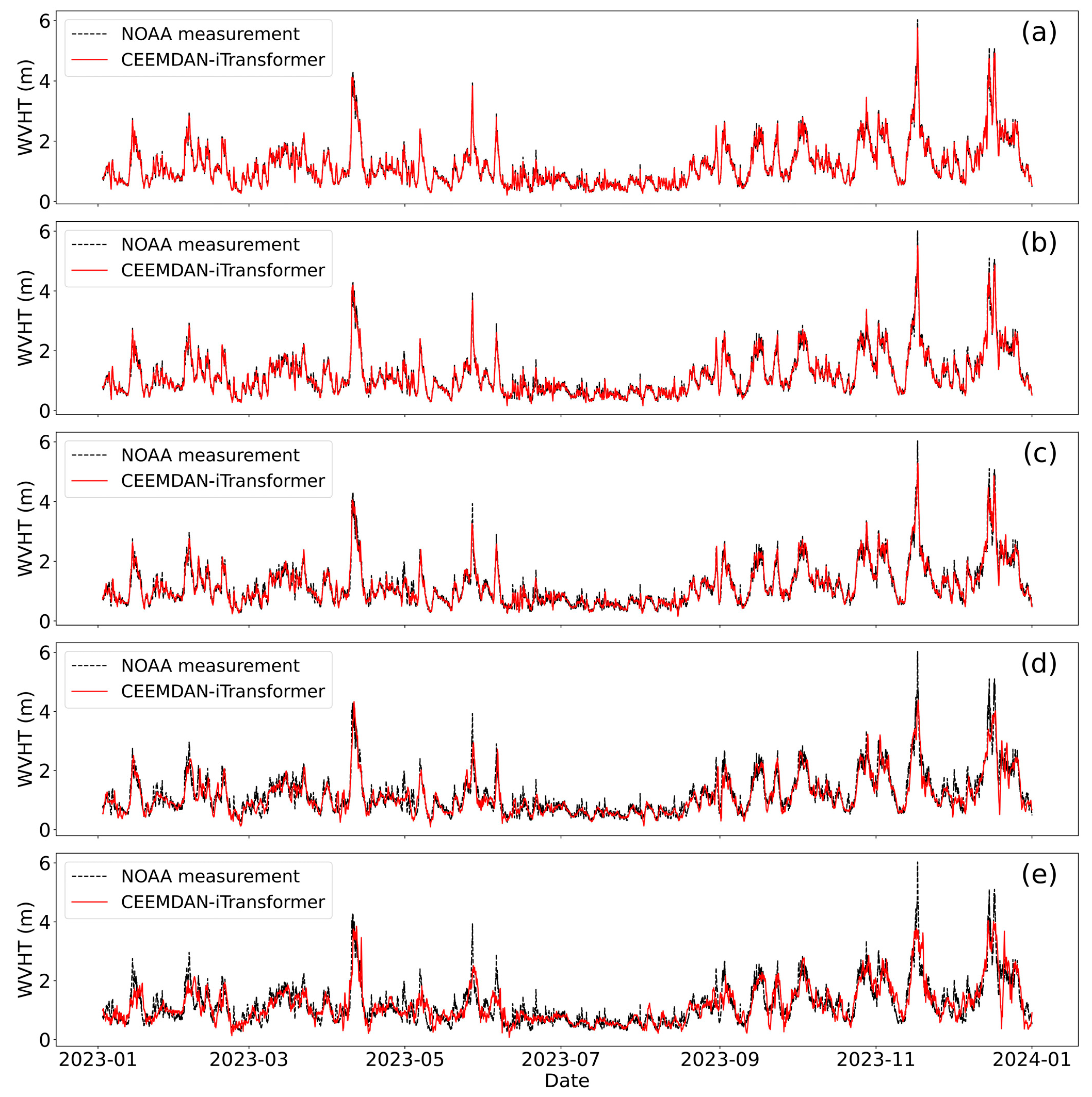
Figure 11 shows a comparison of the CEEMDAN-iTransformer model’s predicted WVHT with actual observations for the buoy 41009 test dataset across different forecast horizons. The test dataset spans one year, during which WVHT varied broadly between 0.5 and 6 m, reflecting the typical characteristics of an oceanic environment. As shown in the figure, for 3 h, 6 h, and 12 h forecasts, the model outputs fit the observed data well. The model accurately captures the trends in WVHT, whether for small fluctuations under steady conditions or sudden surges in wave height under extreme weather conditions. As the forecast horizon is extended to 24 h and 48 h, the forecast accuracy shows a certain decline, manifested as increased deviations and slight shifts in wave peak positions. This is primarily due to the gradual accumulation of errors in the forecast. However, even under longer-term forecast scenarios, the CEEMDAN-iTransformer model is still able to capture the overall evolution trend of WVHT, demonstrating strong time-series modeling capabilities and generalization performance.

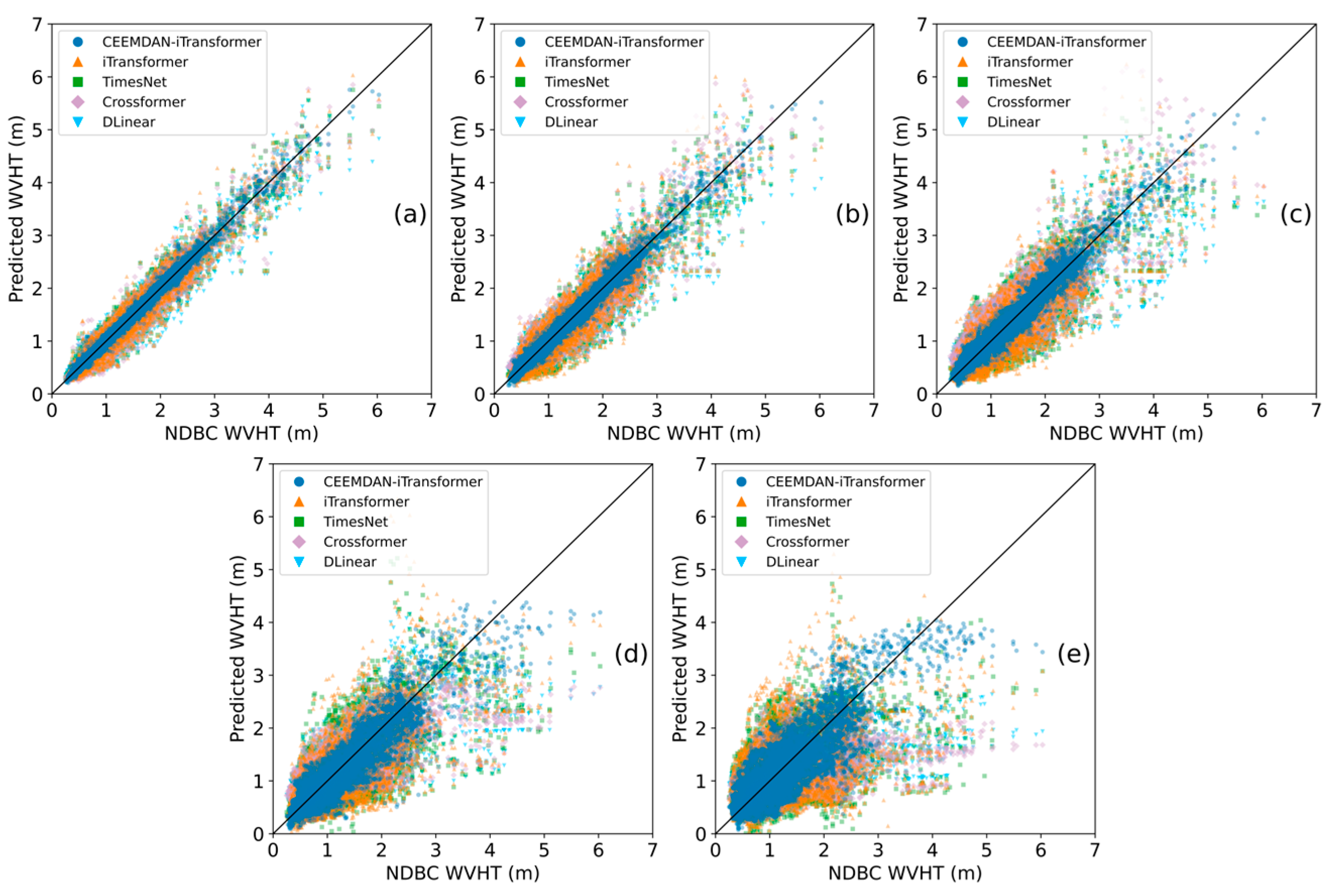
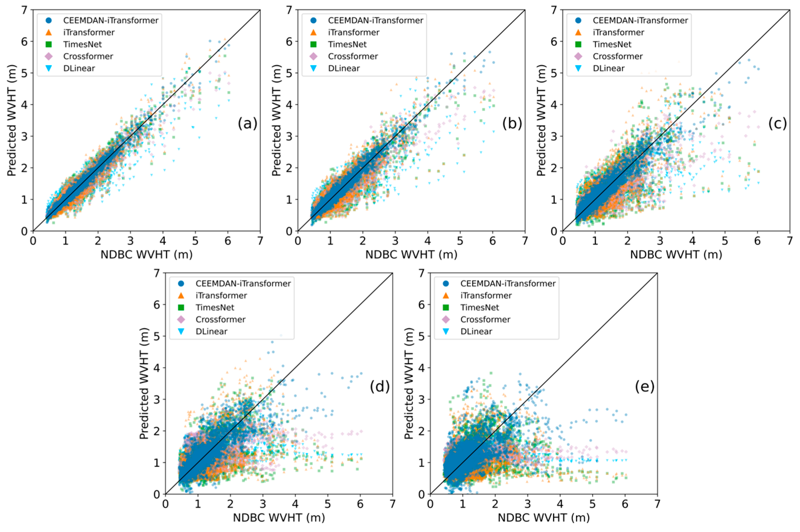
Figure 12 visually illustrates the relationship between observed WVHT and the predicted values from various models using a scatter plot. Each sub-figure corresponds to a specific forecast period, with the x-axis representing the WVHT observed by buoys and the y-axis showing the prediction results from each model. Scatter points of different colors represent the predicted values from different models, while the black diagonal line represents the ideal scenario where predicted and observed values are perfectly aligned. The proximity of the scatter points to the diagonal line reflects the accuracy of the model’s predictions; the closer the points are to the diagonal, the smaller the prediction error.

As shown in Figure 12, the scatter points for the CEEMDAN-iTransformer model are the most concentrated, with most points clustered closely around the diagonal line. This performance is particularly notable in shorter-term forecasts, indicating that the model possesses strong fitting capabilities in capturing fluctuations in WVHT. As the forecast horizon increases, the prediction errors of all models increase, and the scatter plots become more dispersed. However, the CEEMDAN-iTransformer model still maintains a distribution that remains relatively close to the diagonal line. In contrast, the scatter plots of other models are more dispersed, exhibiting significant underestimation or overestimation in longer-term forecasts. Overall, by combining signal decomposition with deep learning, the CEEMDAN-iTransformer model effectively improves prediction accuracy and stability across different forecast horizons, demonstrating its application potential and robustness for WVHT forecasting in marine environments.

4.2.2. Prediction Results of Buoy 41004

Table 5. Comparison of errors from various models at buoy 41004 for different forecast durations.

Forecast Hours	Metrics	CEEMDAN-iTransformer	iTransformer	TimesNet	Crossformer	DLinear
3 h	MAE (m) ↓	0.0579	0.1283	0.1266	0.1205	0.1740
	RMSE (m) ↓	0.0883	0.2024	0.1997	0.1980	0.2809
	MAPE (%) ↓	4.3242	9.4641	9.3588	9.1032	13.7274
	CC ↑	0.9923	0.9595	0.9603	0.9642	0.9219
6 h	MAE (m) ↓	0.0867	0.2030	0.2077	0.1789	0.2392
	RMSE (m) ↓	0.1299	0.3343	0.3405	0.2937	0.3842
	MAPE (%) ↓	6.6754	14.8554	15.3861	13.0191	19.3408
	CC ↑	0.9836	0.8869	0.8854	0.9159	0.8467
12 h	MAE (m) ↓	0.1446	0.3074	0.3098	0.2772	0.3302
	RMSE (m) ↓	0.2206	0.4891	0.4858	0.4412	0.5122
	MAPE (%) ↓	11.5859	22.7638	23.2404	20.6317	27.6509
	CC ↑	0.9547	0.7443	0.7547	0.7938	0.7006
24 h	MAE (m) ↓	0.2566	0.4370	0.4438	0.3984	0.4351
	RMSE (m) ↓	0.3735	0.6667	0.6598	0.6163	0.6268
	MAPE (%) ↓	20.5988	33.6676	35.1283	30.3631	40.0141
	CC ↑	0.8691	0.5157	0.5098	0.5390	0.4818
48 h	MAE (m) ↓	0.4020	0.5676	0.5594	0.4725	0.4898
	RMSE (m) ↓	0.5986	0.8051	0.7733	0.6647	0.6960
	MAPE (%) ↓	31.9378	44.1171	45.3149	43.5686	43.3805
	CC ↑	0.6531	0.2404	0.2675	0.3712	0.2410

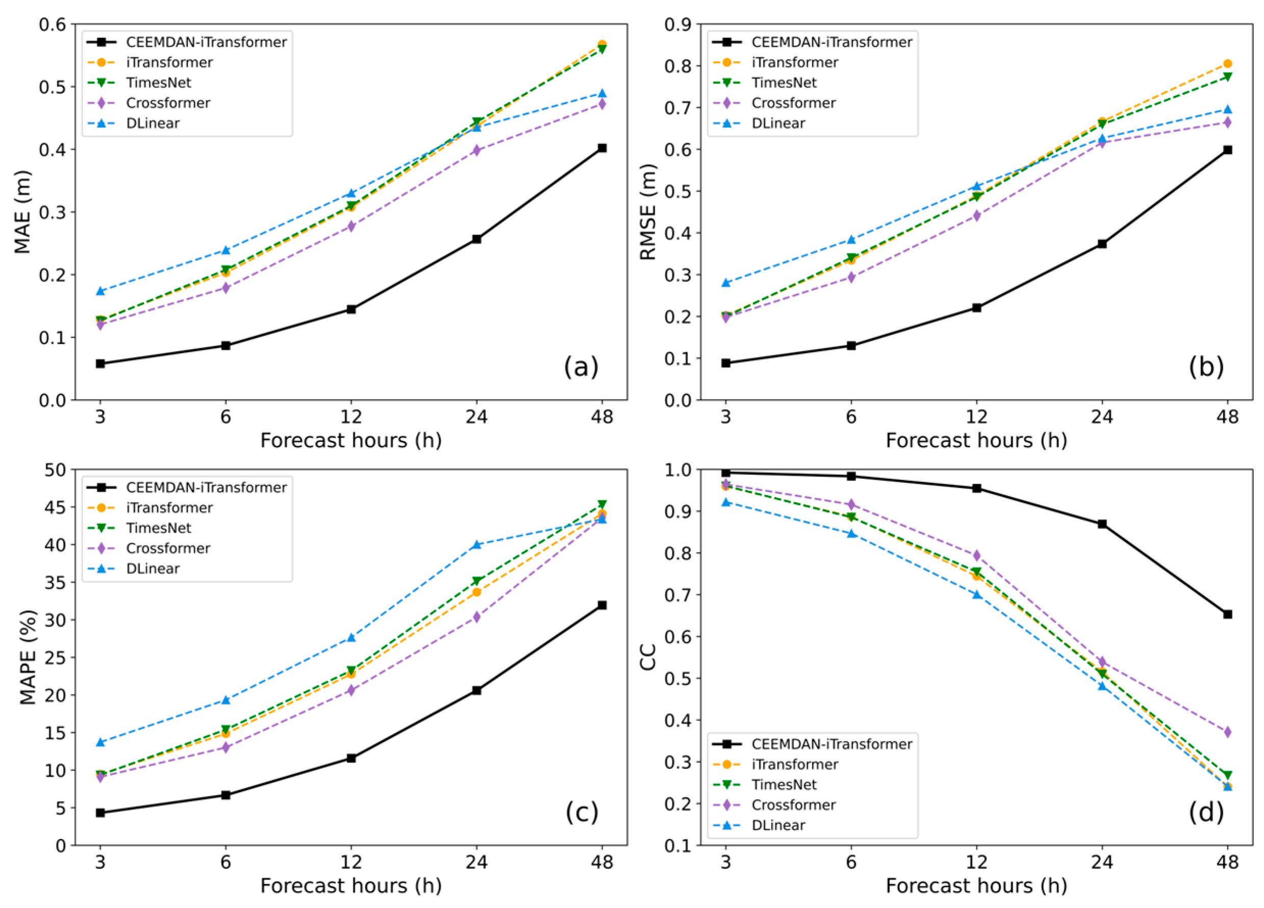
“↓” indicates that a lower value of the evaluation metric corresponds to better model performance, whereas “↑” indicates that a higher value of the evaluation metric corresponds to better model performance.

lists the error evaluation results for each model at buoy 41004, while Figure 13 visually illustrates the overall trend of each model’s performance metrics as a function of forecast horizon using a line chart. During the 3 h, 6 h, and 12 h forecast periods, the prediction errors of the CEEMDAN-iTransformer model increased gradually with forecast duration, but the overall rate of increase was relatively moderate. Specifically, the RMSE increased from 0.0883 m at 3 h to 0.2206 m at 12 h, while the MAPE rose from 4.3242% to 11.5859%. In contrast, the error growth for the other models is more pronounced over the same forecast horizons, particularly for the DLinear model, whose RMSE and MAPE reach 0.5122 m and 27.6509%, respectively, in the 12 h forecast. Overall, the RMSE and MAPE of the CEEMDAN-iTransformer were reduced by approximately 50% to 68.57% and 43.84% to 68.50%, respectively, compared to other models, highlighting the significant advantage of combining signal decomposition with a deep forecasting framework in reducing prediction errors. As the forecast horizon was extended to 24 h and 48 h, the prediction errors of all models generally increased, primarily due to the accumulation of errors over time. At these stages, the CEEMDAN-iTransformer model achieved RMSEs of 0.3735 m and 0.5986 m, with corresponding MAPEs of 20.5988% and 31.9378%. Despite the increase in error, its RMSE and MAPE are still 9.94% to 43.98% and 26.38% to 48.52% lower, respectively, compared to other models. In terms of the CC metric, the CEEMDAN-iTransformer model maintains the highest correlation across all forecast horizons. For example, its CC value reaches 0.9923 in the 3 h forecast, and even in the 48 h forecast, the CC remains at 0.6531, whereas the CC values for the iTransformer and DLinear models have dropped to 0.2404 and 0.2410, respectively.

Referring to Figure 13, we can further observe that the overall performance of the models ranks as follows: CEEMDAN-iTransformer > Crossformer > iTransformer ≈ TimesNet > DLinear. It should be noted that although Crossformer performs slightly better than iTransformer on some metrics, its computational complexity and time consumption are relatively higher. Therefore, in modeling schemes that balance prediction accuracy and computational efficiency, iTransformer still holds significant practical value as a foundational prediction framework, which further highlights the rationality and effectiveness of introducing the CEEMDAN signal decomposition strategy based on it.

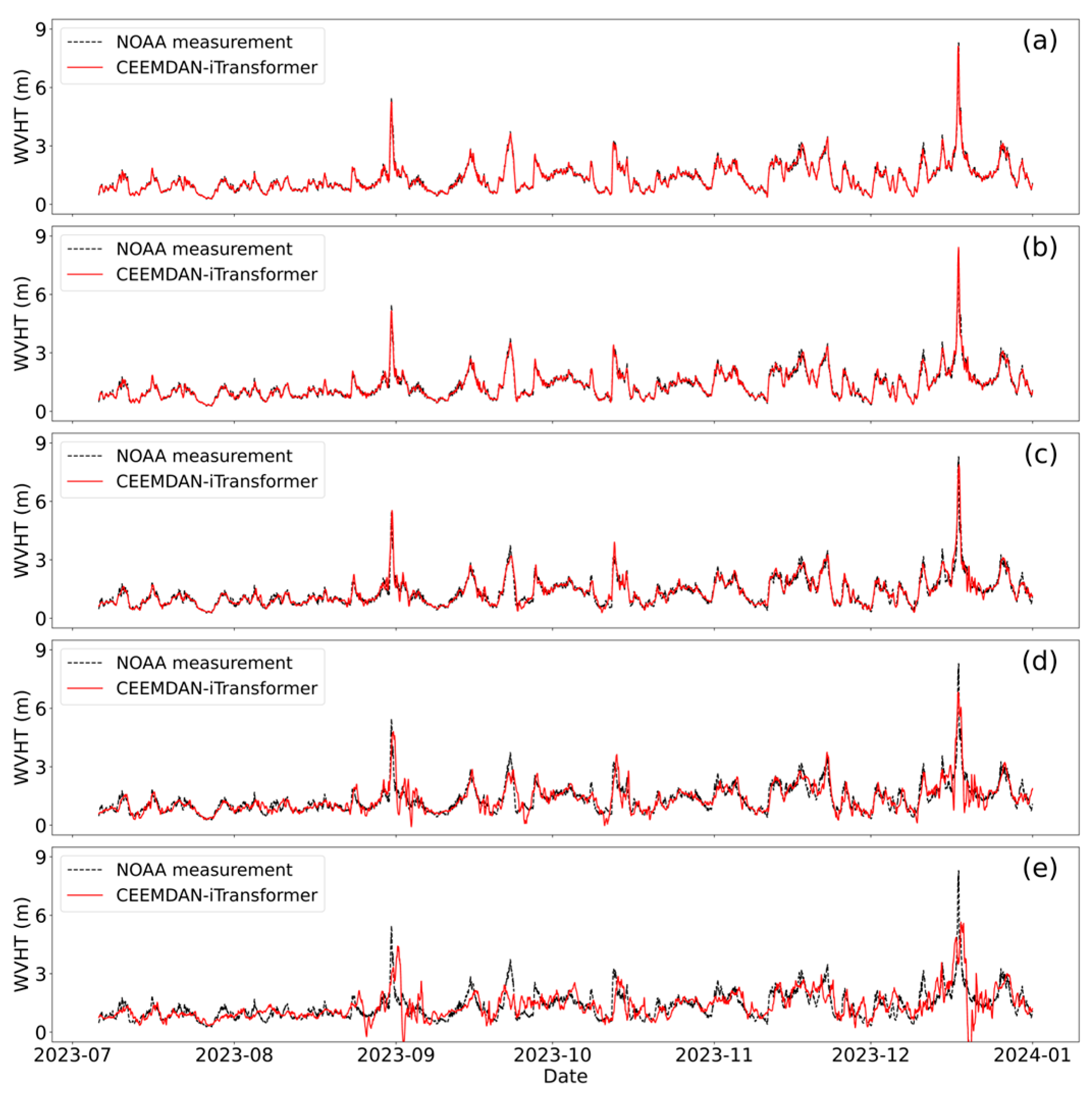
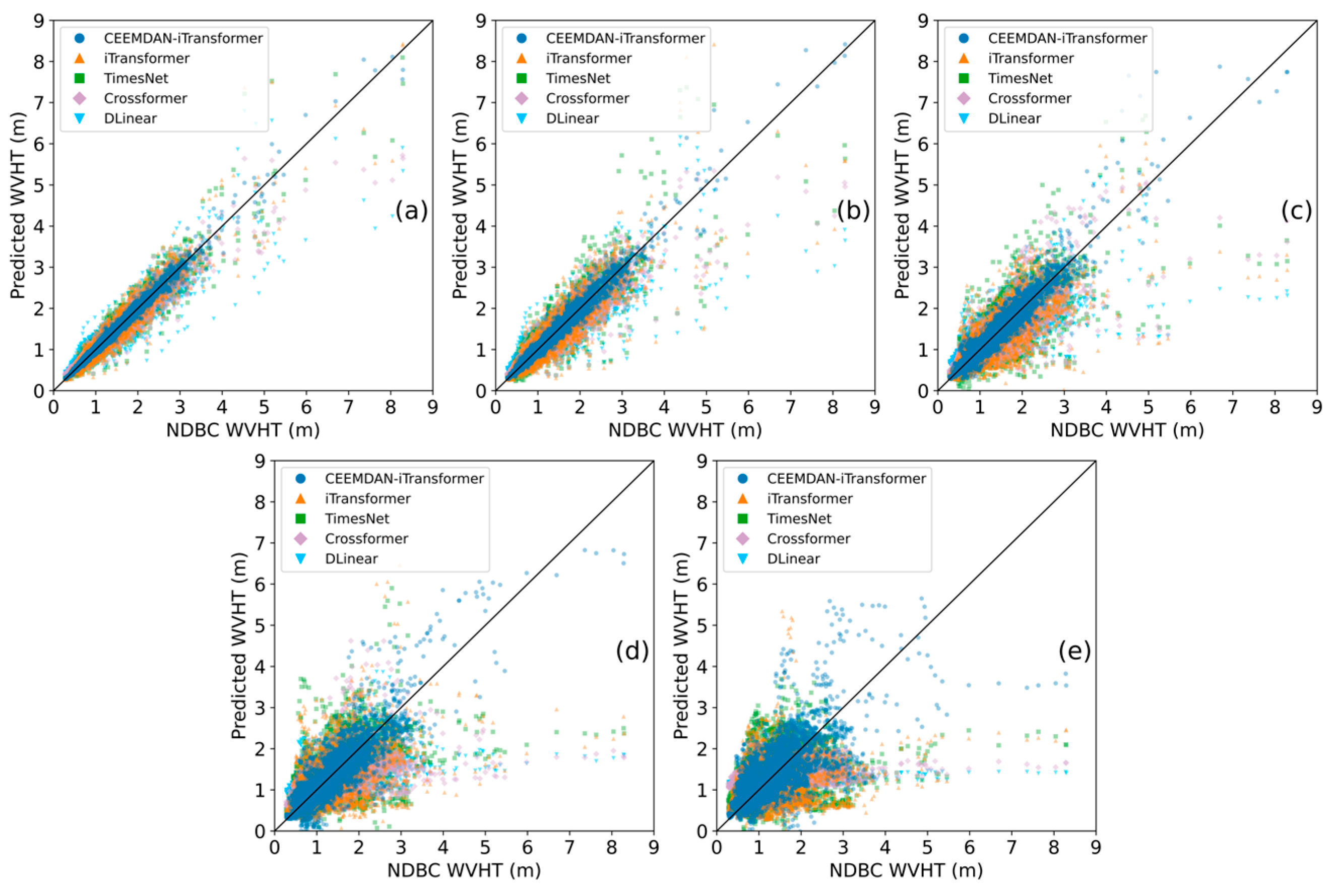
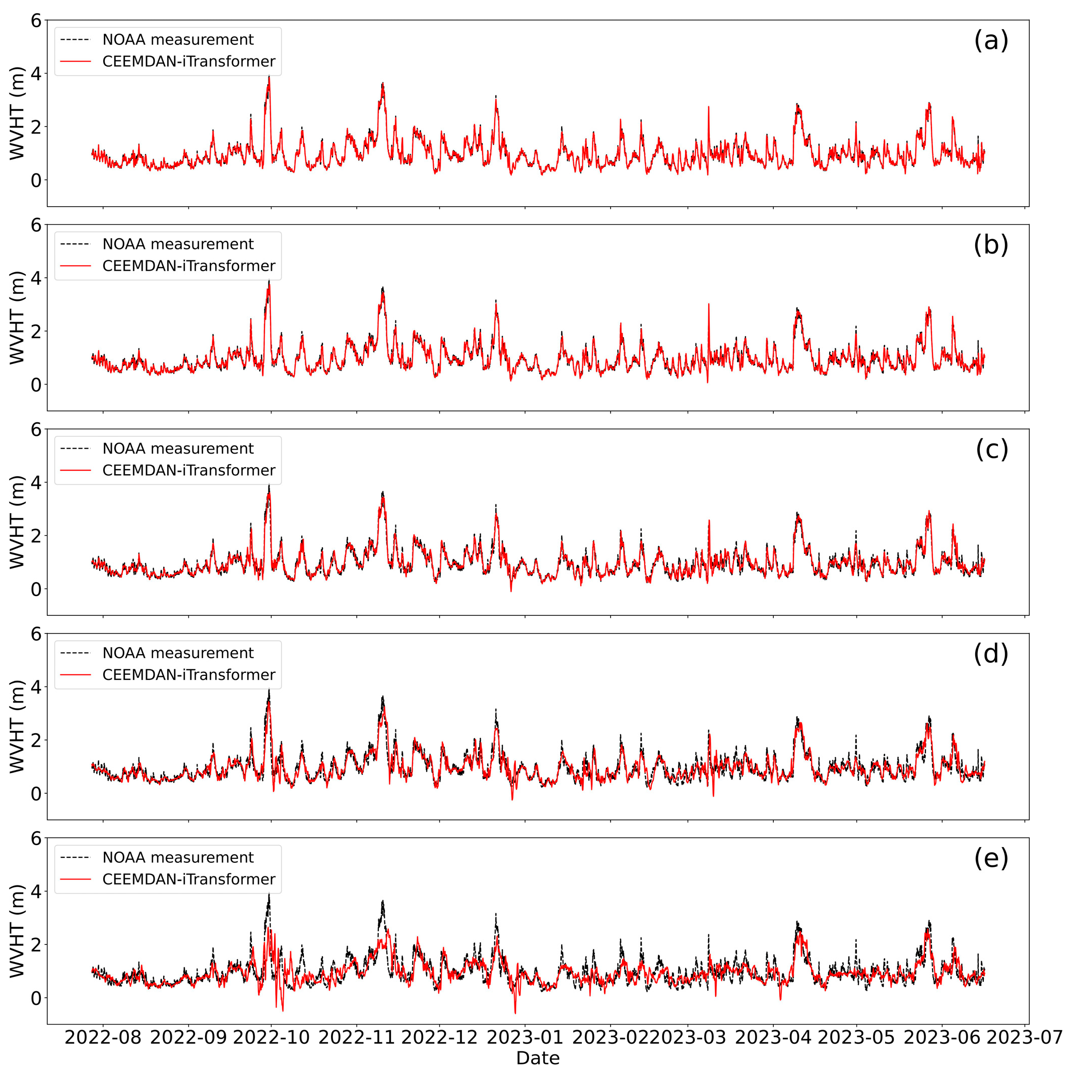
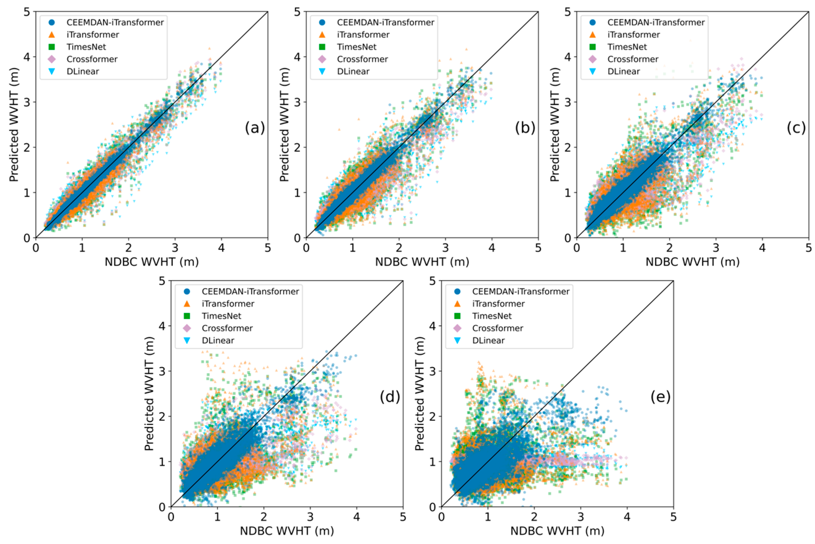
Figure 14 shows a comparison of the CEEMDAN-iTransformer model’s predicted WVHT with observed values for the buoy 41004 test dataset across different forecast horizons. The test data from this buoy spans approximately six months, with WVHT ranging from 0.5 m to 9 m, indicating significant variability. The figure demonstrates that the model fits the observed values well for shorter forecast horizons. As the forecast horizon increases, the prediction accuracy declines slightly. However, even in the 48 h forecast, the model still accurately captures the overall trend of WVHT. Furthermore, Figure 15 compares the prediction accuracy of various models across different forecast horizons using a scatter plot. The results indicate that, in the experiments at this buoy station, the CEEMDAN-iTransformer model continues to perform best.

4.2.3. Prediction Results of Buoy 41008

Table 6. Comparison of errors from various models at buoy 41008 for different forecast durations.

Forecast Hours	Metrics	CEEMDAN-iTransformer	iTransformer	TimesNet	Crossformer	DLinear
3 h	MAE (m) ↓	0.0418	0.0977	0.0938	0.0879	0.1151
	RMSE (m) ↓	0.0587	0.1411	0.1355	0.1229	0.1639
	MAPE (%) ↓	4.6544	10.4263	10.0785	9.9410	12.7158
	CC ↑	0.9934	0.9617	0.9647	0.9708	0.9478
6 h	MAE (m) ↓	0.0627	0.1558	0.1481	0.1474	0.1695
	RMSE (m) ↓	0.0894	0.2270	0.2140	0.2062	0.2400
	MAPE (%) ↓	7.0562	16.5691	15.8744	16.8778	18.9626
	CC ↑	0.9848	0.8997	0.9099	0.9176	0.8844
12 h	MAE (m) ↓	0.0974	0.2233	0.2232	0.2100	0.2322
	RMSE (m) ↓	0.1367	0.3281	0.3233	0.2920	0.3261
	MAPE (%) ↓	11.2678	23.4049	23.8868	24.2076	26.5314
	CC ↑	0.9640	0.7858	0.7876	0.8208	0.7743
24 h	MAE (m) ↓	0.1668	0.3237	0.3215	0.2915	0.3086
	RMSE (m) ↓	0.2331	0.4659	0.4612	0.4078	0.4233
	MAPE (%) ↓	19.3189	34.6239	34.3517	33.5351	37.0725
	CC ↑	0.8914	0.5306	0.5304	0.6051	0.5673
48 h	MAE (m) ↓	0.2699	0.4098	0.4026	0.3666	0.3551
	RMSE (m) ↓	0.3825	0.5804	0.5710	0.5025	0.4975
	MAPE (%) ↓	30.5918	44.7483	44.0290	45.8322	42.9021
	CC ↑	0.6816	0.2392	0.2245	0.1945	0.2360

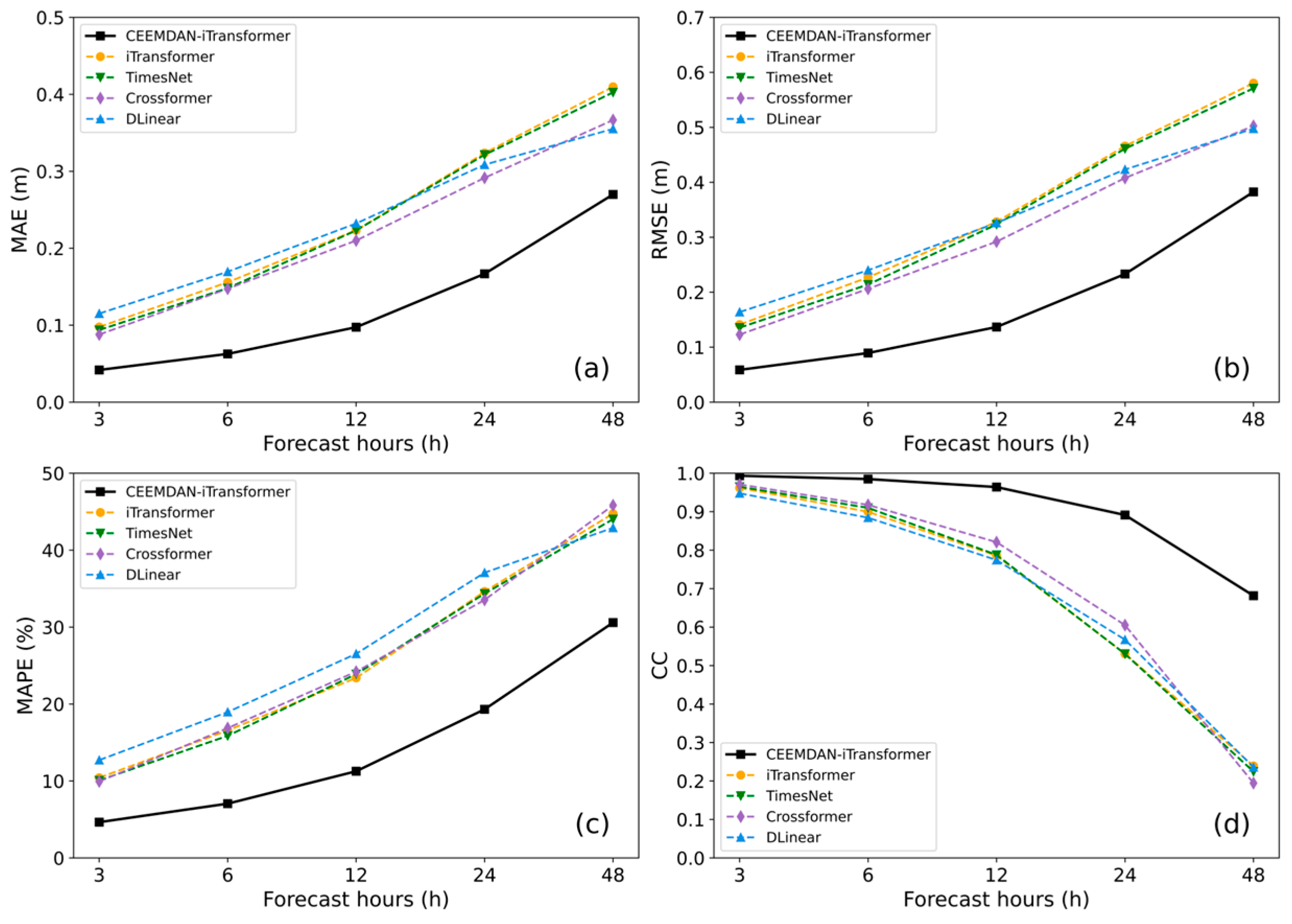
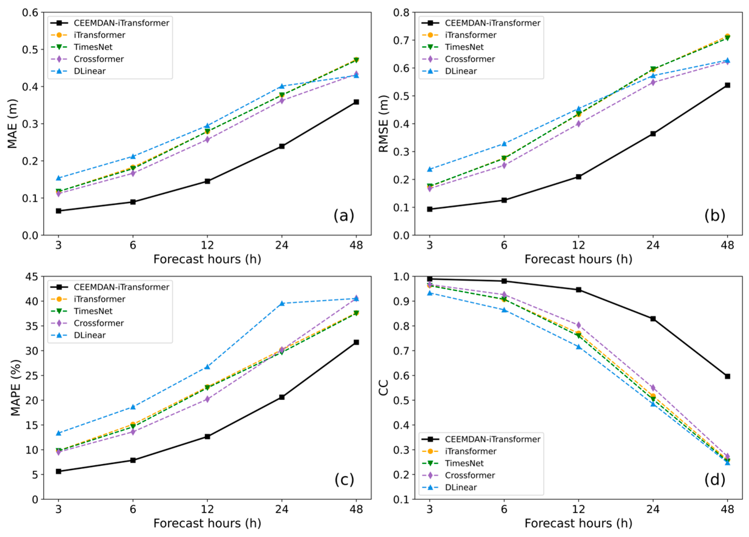
“↓” indicates that a lower value of the evaluation metric corresponds to better model performance, whereas “↑” indicates that a higher value of the evaluation metric corresponds to better model performance.

presents the detailed values of MAE, RMSE, MAPE, and CC for buoy 41008, while Figure 16 illustrates the corresponding trends of these metrics with increasing forecast horizons. According to Table 6, for 3 h, 6 h and 12 h forecasts, the prediction errors of CEEMDAN-iTransformer increase gradually but remain at a relatively low level. Specifically, MAE rises from 0.0418 m to 0.0974 m, RMSE increases from 0.0587 m to 0.1367 m, and MAPE grows from 4.6544% to 11.2678%, while CC decreases slightly from 0.9934 to 0.9640. Compared with other models, CEEMDAN-iTransformer consistently achieves the lowest errors and highest correlation, with MAE reduced by 52.45–63.68% and RMSE reduced by approximately 55–65%, while CC improves by 2.33–24.50%, demonstrating its strong short-term prediction capability. For 24 h and 48 h forecasts, all models exhibit increased errors and decreased CC due to error accumulation. Nevertheless, CEEMDAN-iTransformer still maintains a clear advantage. Its MAE reaches 0.1668 m and 0.2699 m, RMSE reaches 0.2331 m and 0.3825 m, and MAPE increases to 19.3189% and 30.5918%, while CC remains relatively high at 0.8914 and 0.6816. In comparison, other models show significantly larger errors and sharper declines in CC. Overall, CEEMDAN-iTransformer reduces MAE by 23.99–48.47% and RMSE by about 20–45%, while improving CC by 47.32–250.44%. Figure 16 further confirms that CEEMDAN-iTransformer consistently outperforms the baseline models across all metrics and forecast horizons, highlighting its robustness and effectiveness.

Figure 17 shows a comparison of the CEEMDAN-iTransformer model’s predicted WVHT with observed values for the buoy 41008 test dataset across different forecast horizons. Figure 18 presents a scatter plot comparing the forecasting outcomes of various models for buoy 41008 against NDBC measured data. The figure shows that the CEEMDAN-iTransformer model’s scatter distribution is the most concentrated, with the majority of points closely aligned with the diagonal line. As the forecast period extends, the prediction errors increase, and the scatter distribution becomes more dispersed. Nevertheless, even at longer forecast horizons, the CEEMDAN-iTransformer model outperforms others. In conclusion, the prediction results for buoy 41008 further confirm the superior performance of the CEEMDAN-iTransformer model, especially its significant accuracy advantage in short-term predictions.

4.2.4. Prediction Results of Buoy 44009

Table 7. Comparison of errors from various models at buoy 44009 for different forecast durations.

Forecast Hours	Metrics	CEEMDAN-iTransformer	iTransformer	TimesNet	Crossformer	DLinear
3 h	MAE (m) ↓	0.0653	0.1171	0.1176	0.1121	0.1540
	RMSE (m) ↓	0.0932	0.1745	0.1757	0.1675	0.2368
	MAPE (%) ↓	5.6264	9.7986	9.7973	9.5403	13.3755
	CC ↑	0.9895	0.9635	0.9624	0.9670	0.9331
6 h	MAE (m) ↓	0.0893	0.1828	0.1791	0.1666	0.2121
	RMSE (m) ↓	0.1254	0.2772	0.2755	0.2506	0.3285
	MAPE (%) ↓	7.8748	15.1271	14.6155	13.6179	18.6517
	CC ↑	0.9810	0.9064	0.9076	0.9262	0.8649
12 h	MAE (m) ↓	0.1451	0.2788	0.2792	0.2575	0.2950
	RMSE (m) ↓	0.2095	0.4333	0.4352	0.3999	0.4545
	MAPE (%) ↓	12.6521	22.6893	22.5019	20.2095	26.7657
	CC ↑	0.9459	0.7703	0.7596	0.8031	0.7160
24 h	MAE (m) ↓	0.2392	0.3774	0.3769	0.3624	0.4012
	RMSE (m) ↓	0.3641	0.5941	0.5960	0.5483	0.5726
	MAPE (%) ↓	20.6086	30.1850	29.6572	30.1518	39.5577
	CC ↑	0.8288	0.5170	0.5032	0.5501	0.4848
48 h	MAE (m) ↓	0.3585	0.4726	0.4706	0.4334	0.4299
	RMSE (m) ↓	0.5382	0.7141	0.7069	0.6235	0.6282
	MAPE (%) ↓	31.6896	37.6329	37.5453	40.5581	40.5337
	CC ↑	0.5962	0.2589	0.2533	0.2728	0.2480

“↓” indicates that a lower value of the evaluation metric corresponds to better model performance, whereas “↑” indicates that a higher value of the evaluation metric corresponds to better model performance.

provides the MAE, RMSE, MAPE, and CC values for buoy 44009, while Figure 19 visualizes the variation trends of these evaluation metrics with increasing forecast horizons. According to Table 7, for 3 h, 6 h and 12 h forecasts, the prediction errors of CEEMDAN-iTransformer increase gradually but remain significantly lower than those of other models. Specifically, RMSE rises from 0.0932 m to 0.2095 m, and MAPE increases from 5.6264% to 12.6521%, while CC decreases slightly from 0.9895 to 0.9459. Compared with the baseline models, CEEMDAN-iTransformer reduces RMSE by 44.36–61.83% and MAPE by 37.40–57.94%, while maintaining the highest correlation, demonstrating its superior short-term prediction accuracy and stability. For 24 h and 48 h, all models exhibit increased errors and decreased CC due to error accumulation. Nevertheless, CEEMDAN-iTransformer still achieves the best overall performance. Its RMSE reaches 0.3641 m and 0.5382 m, with corresponding MAPE values of 20.6086% and 31.6896%, while CC remains relatively high at 0.8288 and 0.5962. In comparison, other models show larger errors and more rapid degradation in correlation. Overall, CEEMDAN-iTransformer reduces RMSE by 13.68–38.91% and MAPE by 15.60–47.90%, indicating its robustness and effectiveness in both short- and long-term forecasting scenarios.

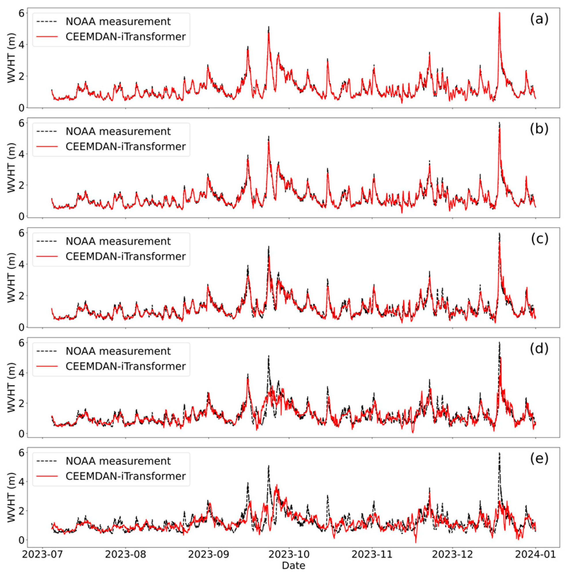
Figure 20 shows a comparison between the CEEMDAN-iTransformer forecast results at various forecast horizons and the time series profile of NDBC measured data for the buoy 44009 test dataset. Figure 21 shows the scatter plot for this buoy station. The test dataset spans approximately six months, during which the WVHT exhibits significant fluctuations, with multiple extreme values observed. From Figure 20, it is evident that in the first three forecast horizons, the model accurately captures the WVHT variation trends, with predicted values closely aligning with the measured data. Even in extreme cases where WVHT approaches 6 m, the model maintains relatively low prediction errors. However, as the forecast horizon extends to 24 h and 48 h, deviations between predicted and observed values become more pronounced. For wave heights in the mid-to-low range (below 4 m), the model continues to capture most trend characteristics effectively. Nevertheless, in extreme WVHT scenarios, the model’s performance is constrained by the forecast duration, making it challenging to accurately predict peak values.

The degradation of forecasting performance at longer prediction horizons is not solely attributable to error accumulation. From a physical perspective, this phenomenon is also associated with the progressive decoupling between wind forcing and wave response, particularly under rapidly evolving atmospheric conditions. As the forecast lead time increases, the direct dynamical linkage between local wind fields and wave growth weakens, leading to reduced physical consistency in wind–wave interactions. In addition, the multivariate input space may suffer from loss of temporal coherence, where correlated features such as wind speed, wind direction, and wave energy components gradually diverge in their joint evolution. This loss of coherence reduces the effectiveness of learned cross-variable dependencies in data-driven models, thereby amplifying prediction uncertainty. Consequently, both physical decoupling and multivariate correlation degradation jointly contribute to the observed decline in long-horizon forecasting accuracy.

4.3. Prediction Capabilities for Storms

4.3.1. Buoy 41004: Major Hurricane Idalia and Winter Storm Event

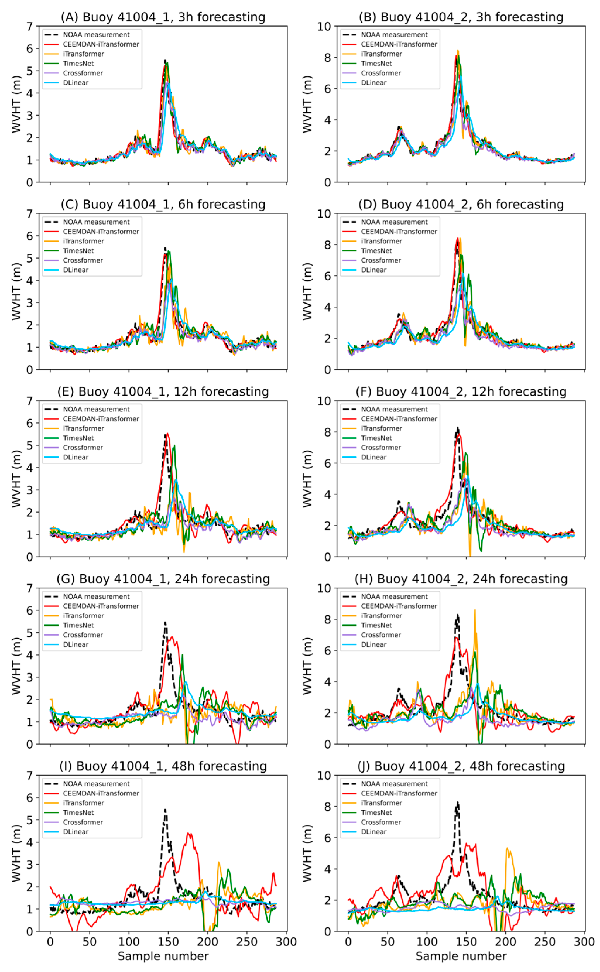
This section highlights the predictive capability of the CEEMDAN-iTransformer model for extreme WVHT events caused by storms. Figure 22 compares the WVHT predictions from various models with NDBC measured values during two storm events in the test set for buoy 41004. The left subplots cover the period from 25 August to 6 September 2023, when Major Hurricane Idalia swept through the area where buoy 41004 is located. The right subplots correspond to the period from 12 to 24 December 2023, during which buoy 41004 experienced a severe winter storm.

Historical data for Major Hurricane Idalia is sourced from the National Hurricane Center (NHC, https://www.nhc.noaa.gov/(accessed on 19 July 2024)), which provides storm records, including paths, intensities, and dates of occurrence. According to NHC, Idalia occurred from 26 to 31 August 2023, reaching a maximum wind speed of 115 kt and a minimum central pressure of 942 mb. As shown in Figure 1, Idalia originated in the Eastern Pacific and made landfall in Florida. Moving northeast, Idalia brought strong winds and storm surges to coastal areas of South Carolina, where buoy 41004 was located in the core affected marine region. A winter storm is an extreme weather phenomenon occurring between November and March, commonly affecting the northern and eastern United States. It is typically triggered by the convergence of cold and moist air. In coastal areas, winter storms can cause significant increases in WVHT, leading to rapid and intense fluctuations. These complex and extreme weather conditions pose a significant challenge for WVHT forecasting and serve as a crucial test for evaluating model predictive capabilities.

The comparison results in Figure 22 show that the CEEMDAN-iTransformer model effectively captures the overall trends and peaks in WVHT during extreme weather events, with its forecast curves closely matching the observed data. The CEEMDAN-iTransformer demonstrates exceptionally high forecast accuracy for 3 h, 6 h, and 12 h forecasts. iTransformer and TimesNet also performed well in the 3 h forecast, while Crossformer and DLinear exhibited varying degrees of deviation starting from the 3 h forecast. As the forecast horizon extended to 12 h, the prediction accuracy of all four comparison models declined overall. In the 24 h and 48 h forecasts, iTransformer and TimesNet significantly underestimated the wave peak values for both storm events, failing to fully reflect the characteristics of extreme variations; Crossformer and DLinear exhibited a smoothing trend in their predictions, causing both wave peaks and troughs to deviate from observed values. Although CEEMDAN-iTransformer exhibited some lag and bias in the 48 h forecast, its overall performance remained significantly superior to that of the other models. This comparison further validates CEEMDAN-iTransformer’s exceptional capability in handling complex nonlinear wave dynamics, particularly demonstrating high stability and accuracy in forecasting extreme weather events.

4.3.2. Buoy 44009: Tropical Storm Ophelia and Winter Storm Event

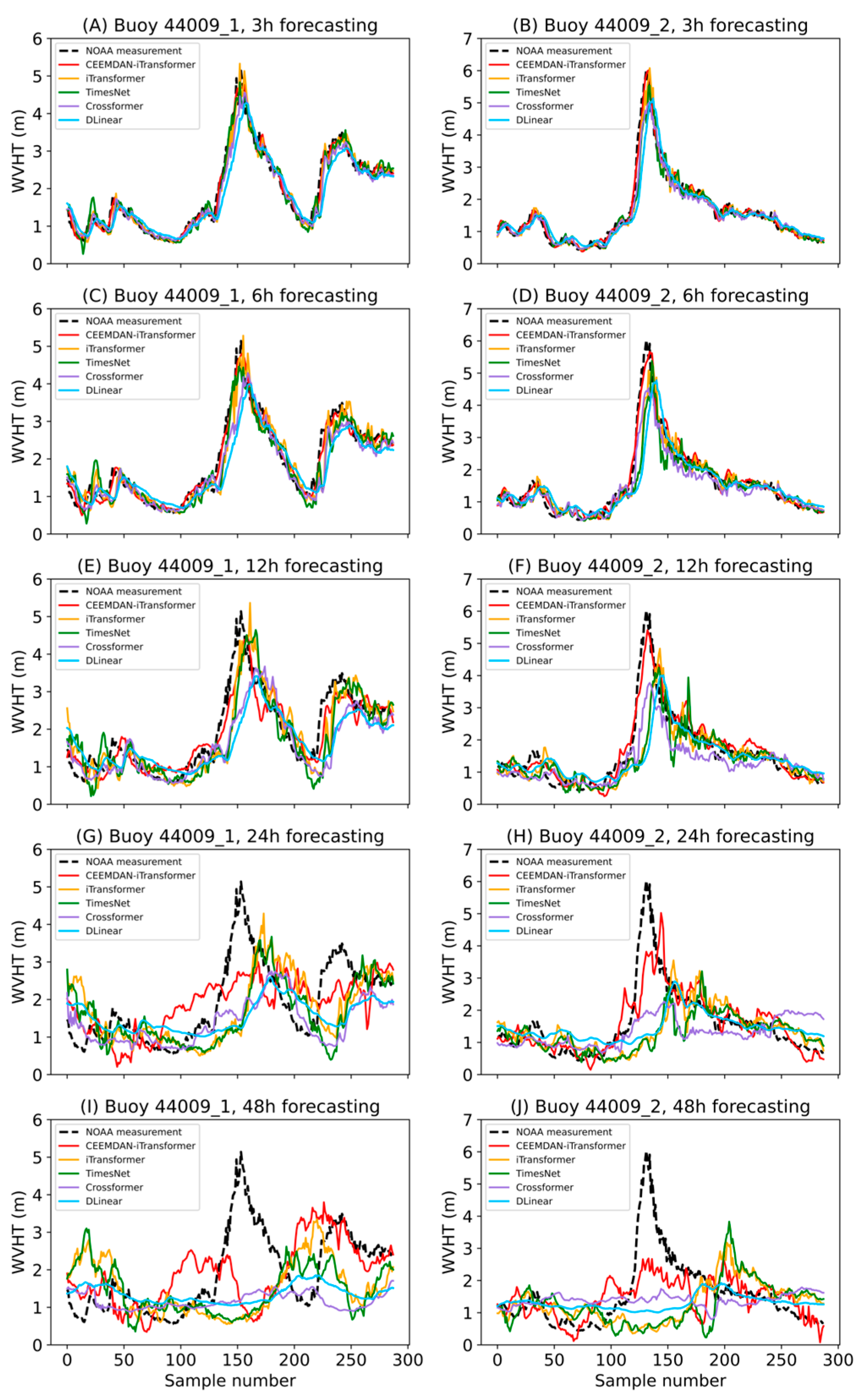
Figure 23 compares WVHT predictions from various models with NDBC measurements during two storm events in the test set for buoy 44009. The left subplots cover the period from 17 to 29 September 2023, when Tropical Storm Ophelia impacted the area surrounding buoy 44009. The right subplots span 13–25 December 2023, during which buoy 44009 experienced a severe winter storm.

According to NHC, Tropical Storm Ophelia occurred from 22 to 23 September 2023, reaching a maximum wind speed of 60 kt and a minimum central pressure of 981 mb. As shown in Figure 1, Ophelia originated off the southeastern U.S. seaboard and made landfall in eastern North Carolina. After landfall, Ophelia moved inland across New Jersey before dissipating near the U.S. East Coast, where buoy 44009 is located. The two extreme weather events experienced by buoy 44009 further validate the model’s forecasting capability.

As shown in Figure 23, in the short-term forecasts of 3 h and 6 h, most models closely align with NOAA-measured data, while Crossformer and DLinear slightly underestimate peak values. When the forecast horizon extends to 12 h, all models except Crossformer and DLinear perform relatively well in predicting WVHT for Storm Ophelia. However, for the winter storm, only CEEMDAN-iTransformer accurately captures the WVHT peak, while the other models exhibit significant underestimation and lag. In the 24 h forecast, although none of the models fully capture the peak WVHT during Storm Ophelia, they generally reflect the overall trend. For the winter storm, only CEEMDAN-iTransformer effectively reproduces WVHT fluctuations, whereas the other models struggle to predict the main variation patterns and peaks. In the 48 h forecast, severe WVHT fluctuations significantly impact long-term predictive performance. In Figure 23I, CEEMDAN-iTransformer partially captures the fluctuation trend but shows reduced accuracy in reproducing peaks. The other models suffer from more severe underestimation, producing overly smoothed predictions that only capture rough trends. In Figure 23J, none of the models accurately represent the amplitude of extreme fluctuations, leading to excessively smooth predictions that deviate substantially from actual data. Overall, the CEEMDAN-iTransformer model demonstrates exceptional robustness and accuracy in predicting WVHT under extreme weather conditions. Despite some lag and peak deviation in long-term forecasts, it remains a reliable tool for precise WVHT prediction in the North Atlantic region.

5. Conclusions

This study proposes a WVHT forecasting approach that integrates signal decomposition and deep learning, namely the CEEMDAN-iTransformer model. The experimental data is sourced from four NDBC buoys in the North Atlantic region, each providing measurements for eleven ocean environmental variables. By calculating Pearson correlation coefficients among these variables, this study identified WSPD, WDIR, WVHT, APD, MWD, PRES, and WTMP as the selected input features for the model. The experimental setup utilizes past 24 h data as input to predict WVHT at future horizons of 3 h, 6 h, 12 h, 24 h, and 48 h. To comprehensively evaluate the model’s predictive performance, MAE, RMSE, MAPE, and CC were employed as error assessment metrics. Furthermore, the forecasting results of CEEMDAN-iTransformer were compared against those of iTransformer, TimesNet, Crossformer, and DLinear to assess its effectiveness.

Given the significant volatility of the WVHT time series, this study employs the CEEMDAN signal decomposition method to decompose the complex original signal into multiple IMFs along with a residual component. Subsequently, the iTransformer model is utilized to independently model and predict each decomposed component. The iTransformer introduces an innovative Token construction approach for multivariate time series data by independently mapping the complete time series of each variable into a Variate Token. This enhancement enables the Attention Mechanism to more effectively capture the interrelationships between different variables, making it particularly well-suited for predicting oceanic environmental parameters with numerous input features. Experimental results indicate that on test datasets from four NDBC buoys, the CEEMDAN-iTransformer model outperforms all baseline models across all forecasting horizons, demonstrating superior robustness and broad applicability. Notably, in extreme WVHT predictions associated with storms, the model exhibits unique advantages, providing a powerful tool for forecasting WVHT in the North Atlantic Ocean.

Although the CEEMDAN-iTransformer model has demonstrated excellent performance in predicting WVHT, this study still has certain limitations that need further improvement and expansion. Firstly, the prediction target in this study is limited to WVHT, a specific wave-related physical quantity. Future research could expand the scope to incorporate additional oceanic environmental variables, such as APD, MWD, or other key parameters, to facilitate a more comprehensive assessment of ocean dynamics. Second, intelligent wave forecasting models rely heavily on high-quality observational data. Therefore, efforts should be made to strengthen multi-source data fusion by combining satellite remote sensing, radar measurements, and numerical simulation data with buoy observations to construct a more comprehensive multi-source fusion forecast model. This will enhance data completeness and accuracy, thereby providing a more solid foundation for model training. In future work, more diverse real-world application scenarios and practical case studies will be incorporated to further validate the robustness, generalization capability, and practical applicability of the proposed forecasting framework. Addressing these aspects will enhance the model’s applicability and reliability in complex oceanic environments.

References

1. Nicholls, R.J.; Cazenave, A. Sea-level rise and its impact on coastal zones. Science 2010, 328, 1517–1520. [Google Scholar] [CrossRef]
2. Holthuijsen, L.H. Waves in Oceanic and Coastal Waters; Cambridge University Press: Cambridge, UK, 2007. [Google Scholar]
3. The WISE Group; Cavaleri, L.; Alves, J.H.G.M.; Ardhuin, F.; Babanin, A.; Banner, M.; Belibassakis, K.; Benoit, M.; Donelan, M.; Groeneweg, J.; et al. Wave modelling—The state of the art. Prog. Oceanogr. 2007, 75, 603–674. [Google Scholar] [CrossRef]
4. Song, T.; Wang, J.; Huo, J.; Wei, W.; Han, R.; Xu, D.; Meng, F. Prediction of significant wave height based on EEMD and deep learning. Front. Mar. Sci. 2023, 10, 1089357. [Google Scholar] [CrossRef]
5. Sverdrup, H.U.; Munk, W.H. Wind, Sea and Swell: Theory of Relations for Forecasting; H.O. Publication No. 601; Hydrographic Office: Washington, DC, USA, 1947.
6. Pierson, W.J.; Moskowitz, L. A proposed spectral form for fully developed wind seas based on the similarity theory of S.A. Kitaigorodskii. J. Geophys. Res. 1964, 69, 5181–5190. [Google Scholar] [CrossRef]
7. Hasselmann, K.; Barnett, T.P.; Bouws, E.; Carlson, H.; Cartwright, D.E.; Enke, K.; Ewing, J.A.; Gienapp, A.; Hasselmann, D.E.; Kruseman, P.; et al. Measurements of wind-wave growth and swell decay during the Joint North Sea Wave Project (JONSWAP). Dtsch. Hydrogr. Z. 1973, A8. [Google Scholar]
8. WAMDI Group. The WAM model—A third generation ocean wave prediction model. J. Phys. Oceanogr. 1988, 18, 1775–1810. [Google Scholar] [CrossRef]
9. Booij, N.; Ris, R.C.; Holthuijsen, L.H. A third-generation wave model for coastal regions: 1. Model description and validation. J. Geophys. Res. Oceans 1999, 104, 7649–7666. [Google Scholar] [CrossRef]
10. Tolman, H.L. User Manual and System Documentation of WAVEWATCH III Version 3.14; NOAA/NWS/NCEP/MMAB Technical Note 276; National Oceanic and Atmospheric Administration: Camp Springs, MD, USA, 2009; p. 166.
11. Deo, M.C.; Naidu, C.S. Real-time wave forecasting using neural networks. Ocean Eng. 1998, 26, 191–203. [Google Scholar] [CrossRef]
12. Makarynskyy, O. Improving wave predictions with artificial neural networks. Ocean Eng. 2004, 31, 709–724. [Google Scholar] [CrossRef]
13. Mahjoobi, J.; Mosabbebi, M.; Haghshenas, M. Prediction of significant wave height using support vector machines. Ocean Eng. 2008, 35, 339–347. [Google Scholar] [CrossRef]
14. Callens, A.; Morichon, D.; Abadie, S.; Delpey, M.; Liquet, B. Using random forest and gradient boosting trees to improve wave forecast at a specific location. Appl. Ocean Res. 2020, 104, 102339. [Google Scholar] [CrossRef]
15. Fan, S.; Xiao, N.; Dong, S. A novel model to predict significant wave height based on long short-term memory network. Ocean Eng. 2020, 205, 107298. [Google Scholar] [CrossRef]
16. Gao, S.; Huang, J.; Li, Y.; Liu, G.; Bi, F.; Bai, Z. A forecasting model for wave heights based on a long short-term memory neural network. Acta Oceanol. Sin. 2021, 40, 62–69. [Google Scholar] [CrossRef]
17. Wei, Z. Forecasting wind waves in the US Atlantic coast using an artificial neural network model: Towards an AI-based storm forecast system. Ocean Eng. 2021, 237, 109646. [Google Scholar] [CrossRef]
18. Hao, P.; Li, S.; Gao, Y. Significant wave height prediction based on deep learning in the South China Sea. Front. Mar. Sci. 2023, 10, 1113788. [Google Scholar] [CrossRef]
19. Zhou, S.; Xie, W.; Lu, Y.; Wang, Y.; Zhou, Y.; Hui, N.; Dong, C. ConvLSTM-based wave forecasts in the South and East China Seas. Front. Mar. Sci. 2021, 8, 680079. [Google Scholar] [CrossRef]
20. Luo, Q.R.; Xu, H.; Bai, L.H. Prediction of significant wave height in hurricane area of the Atlantic Ocean using the Bi-LSTM with attention model. Ocean Eng. 2022, 266, 112747. [Google Scholar] [CrossRef]
21. Huang, X.; Tang, J.; Shen, Y. Long time series of ocean wave prediction based on PatchTST model. Ocean Eng. 2024, 301, 117572. [Google Scholar] [CrossRef]
22. Kang, X.; Song, H.; Zhang, Z.; Yin, X.; Gu, J. A transformer-based method for correcting significant wave height numerical forecasting errors. Front. Mar. Sci. 2024, 11, 1374902. [Google Scholar] [CrossRef]
23. Mlakar, P.; Ricchi, A.; Carniel, S.; Bonaldo, D.; Ličer, M. DELWAVE 1.0: Deep learning surrogate model of surface wave climate in the Adriatic Basin. Geosci. Model Dev. 2024, 17, 4705–4725. [Google Scholar] [CrossRef]
24. Karbasi, M.; Jamei, M.; Ali, M.; Abdulla, S.; Chu, X.; Yaseen, Z.M. Developing a novel hybrid auto encoder decoder bidirectional gated recurrent unit model enhanced with empirical wavelet transform and Boruta-CatBoost to forecast significant wave height. J. Clean. Prod. 2022, 379, 134820. [Google Scholar] [CrossRef]
25. Wang, Y.; Satake, K.; Maeda, T.; Shinohara, M.; Sakai, S. A method of real-time tsunami detection using ensemble empirical mode decomposition. Seismol. Res. Lett. 2020, 91, 2851–2861. [Google Scholar] [CrossRef]
26. Zhou, S.; Bethel, B.J.; Sun, W.; Zhao, Y.; Xie, W.; Dong, C. Improving significant wave height forecasts using a joint empirical mode decomposition–long short-term memory network. J. Mar. Sci. Eng. 2021, 9, 744. [Google Scholar] [CrossRef]
27. Hao, W.; Sun, X.; Wang, C.; Chen, H.; Huang, L. A hybrid EMD-LSTM model for non-stationary wave prediction in offshore China. Ocean Eng. 2022, 246, 110566. [Google Scholar] [CrossRef]
28. Ji, Q.; Han, L.; Jiang, L.; Zhang, Y.; Xie, M.; Liu, Y. Short-term prediction of the significant wave height and average wave period based on the variational mode decomposition–temporal convolutional network–long short-term memory (VMD–TCN–LSTM) algorithm. Ocean Sci. 2023, 19, 1561–1578. [Google Scholar] [CrossRef]
29. Altunkaynak, A.; Çelik, A.; Mandev, M.B. Hourly significant wave height prediction via singular spectrum analysis and wavelet transform based models. Ocean Eng. 2023, 281, 114771. [Google Scholar] [CrossRef]
30. Ouyang, Z.; Gao, Y.; Zhang, X.; Wu, X.; Zhang, D. Significant wave height forecasting based on EMD-TimesNet networks. J. Mar. Sci. Eng. 2024, 12, 536. [Google Scholar] [CrossRef]
31. Ding, T.; Wu, D.; Li, Y.; Shen, L.; Zhang, X. A hybrid CEEMDAN-VMD-TimesNet model for significant wave height prediction in the South Sea of China. Front. Mar. Sci. 2024, 11, 1375631. [Google Scholar] [CrossRef]
32. Shen, W.; Ying, Z.; Zhao, Y.; Wang, X. Significant wave height prediction in monsoon regions based on the VMD-CNN-BiLSTM model. Front. Mar. Sci. 2024, 11, 1503552. [Google Scholar] [CrossRef]
33. Huang, N.E.; Shen, Z.; Long, S.R.; Wu, M.C.; Shih, H.H.; Zheng, Q.; Yen, N.-C.; Tung, C.C.; Liu, H.H. The empirical mode decomposition and the Hilbert spectrum for nonlinear and nonstationary time series analysis. Proc. R. Soc. Lond. A Math. Phys. Eng. Sci. 1998, 454, 903–995. [Google Scholar] [CrossRef]
34. Wu, Z.; Huang, N.E. Ensemble empirical mode decomposition: A noise-assisted data analysis method. Adv. Adapt. Data Anal. 2009, 1, 1–41. [Google Scholar] [CrossRef]
35. Torres, M.E.; Colominas, M.A.; Schlotthauer, G.; Flandrin, P. A complete ensemble empirical mode decomposition with adaptive noise. In Proceedings of the 2011 IEEE International Conference on Acoustics, Speech and Signal Processing (ICASSP), Prague, Czech Republic, 22–27 May 2011; IEEE: New York, NY, USA, 2011; pp. 4144–4147. [Google Scholar]
36. Vaswani, A.; Shazeer, N.M.; Parmar, N.; Uszkoreit, J.; Jones, L.; Gomez, A.N.; Kaiser, L.; Polosukhin, I. Attention is all you need. In Proceedings of the Neural Information Processing Systems (NeurIPS), Long Beach, CA, USA, 4–9 December 2017; pp. 5998–6008. [Google Scholar]
37. Liu, Y.; Hu, T.; Zhang, H.; Wu, H.; Wang, S.; Ma, L.; Long, M. iTransformer: Inverted Transformers Are Effective for Time Series Forecasting. In Proceedings of the International Conference on Learning Representations (ICLR), Vienna, Austria, 7–11 May 2023. [Google Scholar]
38. Liu, Y.; Yu, B.; Wu, J.; Zhang, X.; Lin, S. TimesNet: A New Paradigm for Time Series Forecasting. In Proceedings of the Thirty-Seventh AAAI Conference on Artificial Intelligence, Washington, DC, USA, 7–14 February 2023; Volume 37, pp. 10322–10330. [Google Scholar]
39. Zhang, Y.; Yan, J. Crossformer: Transformer Utilizing Cross-Dimension Dependency for Multivariate Time Series Forecasting. In Proceedings of the International Conference on Learning Representations (ICLR), Kigali, Rwanda, 1–5 May 2023. [Google Scholar]
40. Zeng, A.; Chen, M.; Zhang, L.; Xu, Q. Are Transformers Effective for Time Series Forecasting? In Proceedings of the Thirty-Seventh AAAI Conference on Artificial Intelligence, Washington, DC, USA, 7–14 February 2023; Volume 37, pp. 11121–11128. [Google Scholar]
Figure 1. The geographical locations of NDBC buoys 44009, 41004, 41008, and 41009.
Jmse 14 00994 g001
Figure 2. WSPD and WDIR rose diagram at buoy stations. (a) 44009; (b) 41004; (c) 41008; (d) 41009.
Jmse 14 00994 g002
Figure 3. WVHT and MWD rose diagrams at buoy stations. (a) 44009; (b) 41004; (c) 41008; (d) 41009.
Jmse 14 00994 g003
Figure 4. The Pearson correlation coefficient matrix of marine environmental variables.
Jmse 14 00994 g004
Figure 5. Example of time series profiles of selected feature variables.
Jmse 14 00994 g005
Figure 6. Comparison of multivariate time series input construction for Transformer and iTransformer models.
Jmse 14 00994 g006
Figure 7. The structure of iTransformer.
Jmse 14 00994 g007
Figure 8. Original time series and signal decomposition results of WVHT at buoy 41009.
Jmse 14 00994 g008
Figure 10. Comparison of the predictive performance of various models at buoy 41009 under different evaluation metrics. (a) MAE, (b) RMSE, (c) MAPE, (d) CC.
Jmse 14 00994 g010
Figure 11. Comparison of predicted results and measured values of the CEEMDAN-iTransformer model at buoy 41009 for different forecast durations. (a) 3 h, (b) 6 h, (c) 12 h, (d) 24 h, (e) 48 h.
Jmse 14 00994 g011
Figure 12. Scatter plots comparing the predicted results of various models with the measured values at buoy 41009 for different forecast durations. (a) 3 h, (b) 6 h, (c) 12 h, (d) 24 h, (e) 48 h.
Jmse 14 00994 g012
Figure 13. Comparison of the predictive performance of various models at buoy 41004 under different evaluation metrics. (a) MAE, (b) RMSE, (c) MAPE, (d) CC.
Jmse 14 00994 g013
Figure 14. Comparison of predicted results and measured values of the CEEMDAN-iTransformer model at buoy 41004 for different forecast durations. (a) 3 h, (b) 6 h, (c) 12 h, (d) 24 h, (e) 48 h.
Jmse 14 00994 g014
Figure 15. Scatter plots comparing the predicted results of various models with the measured values at buoy 41004 for different forecast durations. (a) 3 h, (b) 6 h, (c) 12 h, (d) 24 h, (e) 48 h.
Jmse 14 00994 g015
Figure 16. Comparison of the predictive performance of various models at buoy 41008 under different evaluation metrics. (a) MAE, (b) RMSE, (c) MAPE, (d) CC.
Jmse 14 00994 g016
Figure 17. Comparison of predicted results and measured values of the CEEMDAN-iTransformer model at buoy 41008 for different forecast durations. (a) 3 h, (b) 6 h, (c) 12 h, (d) 24 h, (e) 48 h.
Jmse 14 00994 g017
Figure 18. Scatter plots comparing model predictions at buoy 41008 across five forecast horizons. (a) 3 h, (b) 6 h, (c) 12 h, (d) 24 h, (e) 48 h.
Jmse 14 00994 g018
Figure 19. Comparison of the predictive performance of various models at buoy 44009 under different evaluation metrics. (a) MAE, (b) RMSE, (c) MAPE, (d) CC.
Jmse 14 00994 g019
Figure 20. Comparison of predicted results and measured values of the CEEMDAN-iTransformer model at buoy 44009 for different forecast durations. (a) 3 h, (b) 6 h, (c) 12 h, (d) 24 h, (e) 48 h.
Jmse 14 00994 g020
Figure 21. Scatter plots comparing the predicted results of various models with the measured values at buoy 44009 for different forecast durations. (a) 3 h, (b) 6 h, (c) 12 h, (d) 24 h, (e) 48 h.
Jmse 14 00994 g021
Figure 22. Comparison of predicted results and measured values at buoy 41004 by various models for the Major Hurricane “Idalia” (A,C,E,G,I) and the winter storm (B,D,F,H,J) at different forecast durations. (A,B) 3 h, (C,D) 6 h, (E,F) 12 h, (G,H) 24 h, (I,J) 48. The sample number indicates the time sample number.
Jmse 14 00994 g022
Figure 23. Comparison of predicted results and measured values at buoy 44009 by various models for the Tropical Storm “Ophelia” (A,C,E,G,I) and the winter storm (B,D,F,H,J) at different forecast durations. (A,B) 3 h, (C,D) 6 h, (E,F) 12 h, (G,H) 24 h, (I,J) 48. The sample number indicates the time sample number.
Jmse 14 00994 g023