Hybrid Modeling and Analysis of Offshore Wind Turbines Using an Aero–Servo–Elastic Rotor–Nacelle Superelement

Abstract

An efficient hybrid modeling framework is developed for the dynamic analysis of offshore wind turbines (OWTs) by coupling an aero–servo–elastic rotor–nacelle superelement with a hydroelastic substructure. The complex rotor–nacelle dynamics are condensed into a reduced-order 14-DOF representation through a modal-based multibody formulation, while retaining blade deformation, spinning effects, nonlinear aerodynamic loading, and active servo controls. Its interface compatibility at the nacelle enables the coupling with either numerical or physical substructures, establishing a unified basis for system hybrid formulation, co-simulations, and real-time hybrid simulations. The validity of the superelement is verified by comparing the resulting fully coupled modal model against OpenFAST, demonstrating high consistency in time-domain responses. As a demonstration, the verified superelement is further coupled with a 1D finite element model of the supporting structure (tower–monopile substructure) to form a hybrid model, enabling accurate force analysis of the OWT structure. Dynamic analyses of the IEA 10 MW OWT reveal that while the blade flapwise responses and the operation-related edgewise responses are 1P-dominated, tower side–side responses and idling-related tower fore–aft and blade edgewise responses manifest at their corresponding resonance frequencies. The maximum displacement and maximum bending moment envelopes vary monotonically with height. Instead, the maximum stress envelope possesses high values in the mid-lower sections of the tower. This high-stress region undergoes a spatial shift driven by the blade feathering mechanism.

1. Introduction

Offshore wind energy has developed rapidly owing to its superior wind resources, vast spatial availability, and advantages in transportation and deployment. It is projected that by 2030, the single-unit capacity of offshore wind turbines (OWTs) will reach 35 MW, supported by large-scale rotor diameters exceeding 350 m [1]. While this up-scaling is beneficial for cost reduction and efficiency, it poses significant challenges to the ultimate strength and durability of the structures [2]. Consequently, there is a fundamental need for models—whether physical or computational—that can faithfully capture the dynamic behavior of OWTs to support system response analysis and design optimization.

In terms of physical modeling, extensive scaled experiments have investigated the dynamic characteristics of OWTs with various foundations under individual or combined wind, wave, and current loads [3,4]. Cao et al. (2020) [5] investigated a new 10 MW semi-submersible OWT concept through a basin model test, verifying that its dynamic responses under both operational and extreme conditions at a 60 m water depth meet the safety requirements of current standards. Ren et al. (2024) [6] conducted a basin test to evaluate the impact of the tendon failure on a multi-column tension leg platform OWT, demonstrating that key motion responses, such as surge, heave, and pitch, do not significantly deteriorate following a breakage event. Furthermore, a scaled experiment by Chen et al. (2025) [4] on a 10 MW jacket-type OWT showed that structural responses under coupled wind-wave actions are significantly smaller than the square root of the sum of the squares of their individual effects; while wind loads dominate the mean structural response and suppress vibrations at the first structural frequency and the wave frequency. More recently, Jia et al. (2026) [7] conducted combined wind–current flume experiments, confirming that seabed scour weakens the pile–soil stiffness of monopile-supported OWTs, leading to a notable decrease in the system’s second-order natural frequency and significant changes in its critical structural responses. While physical experiments provide indispensable insights into the complex coupled behaviors of OWTs, they are often constrained by high costs, time consumption, and scaling effects [8]. Complementarily, diverse computational models—from reduced-order analytical formulations to high-fidelity numerical simulations—have been widely developed.

Structural modeling of wind turbines can be primarily achieved through three-dimensional finite elements (3D FEs), equivalent 1D (one-dimensional) beam elements, and the modal-based formulation. The fundamental distinction among these approaches lies in the definition of element degrees of freedom (DOFs) and the assumptions regarding deformation modes. The 3D FE models utilize shell elements to represent the tower and the composite material layups of the blades, occasionally incorporating solid elements at geometrically complex regions such as the blade tip [9]. These FE models can explicitly capture the spanwise-varying geometric features, pre-bend and pre-twist configurations, and the strong anisotropy of composite materials. Consequently, they offer distinct advantages in capturing higher-frequency mode shapes, bending-torsion coupling, spanwise-chordwise coupled deformations, as well as the local structural responses and stress distribution [10,11,12]. However, due to the massive number of DOFs and the prohibitively high modeling and computational costs, the 3D FE models are currently impractical for the extensive load case analyses and parameter iterations required during the design phase. Instead, they generally serve as high-fidelity reference models for stress concentration identification, strength/fatigue verification under critical load cases, and the calibration and validation of lower-order structural models [12].

Equivalent 1D beam models can be further categorized into multi-rigid-body formulations and 1D FE methods, depending on their kinematic representation of structural deformation. The former approximates the structure (particularly wind turbine blades) as a chain of rigid bodies connected via kinematic constraints—such as spherical, universal, or cylindrical joints—augmented with spring and damping elements [13,14,15]. This multi-rigid-body representation significantly reduces the system DOFs while enhancing time-domain computational efficiency [16]. However, it inherently deviates from the continuum mechanics behavior of the structure, rendering the model accuracy highly sensitive to the discretization scheme and joint configurations. In contrast, 1D FE formulations discretize the structural continuum along a reference axis with equivalent sectional properties, in which deformation is distributed within each element and described by shape functions derived from beam theory [17]. Commonly utilized 1D beam formulations include the Euler–Bernoulli, Timoshenko, and geometrically exact beam (GEB) theories. The first two beam theories generally assume small strains and rotations, thus relying on fine spanwise discretization and iterative updates within co-rotational or updated Lagrangian frameworks to capture large displacements [18]. In contrast, the GEB theory utilizes a rigorous, finite-rotation-based kinematic framework that intrinsically captures arbitrarily large displacements, strong axial–shear–bending–torsion couplings, and initial geometric effects [19,20]. Notably, in GEB implementations, the parameterization and independent interpolation of finite rotations can introduce approximation errors and trigger shear locking [21]. Furthermore, maintaining stability during implicit time integration under strong geometric nonlinearity and high flexibility often necessitates conservative time steps [22].

Typically rooted in linear or weakly nonlinear beam/shell theories, the modal-based formulation expresses structural deformations as a linear superposition of a few elastic modes, drastically reducing system DOFs and thus enhancing aeroelastic computational efficiency [23]. Although its kinematic representation is constrained by the pre-selected modal basis—struggling to accurately capture local responses and inter-modal coupling effects under strong geometric nonlinearity—such reduced-order models effectively describe the fundamental dynamic characteristics of the structure within small-to-moderate deformation regimes. Consequently, they are particularly well-suited for mechanism and control strategy investigations, modal analyses, and rapid aeroelastic simulations required for extensive fatigue assessments and design optimization [24,25].

To mitigate the inherent trade-off between experimental or computational cost and local structural fidelity, hybrid modeling for real-time hybrid simulations (RTHSs), system hybrid formulations, and co-simulations has emerged as a promising paradigm built upon the coupling of interacting wind turbine substructures. RTHSs bridge the physical–virtual boundary, utilizing sensor-actuator transfer systems to dynamically couple physical and numerical substructures within a hardware-in-the-loop architecture [26]. Theoretically, the global wind turbine system can be flexibly partitioned into arbitrary combinations of physical and numerical substructures, tailored to specific research objectives. For instance, Zhang et al. [27,28] dynamically coupled a modal-based aero–servo–elastic model with various full-scale tuned liquid dampers. Beyond validating the dampers’ effectiveness, their study highlighted the potential of RTHS frameworks for evaluating complex structural dynamics in large wind turbines. Shifting the RTHS partition boundary to the wind turbine structure itself, Song et al. [29] modeled a monopile-supported OWT by coupling a scaled tower–foundation substructure tested in a wave basin with a modal-based aeroelastic rotor. Sun et al. [8] further analyzed a spar-type OWT by integrating a physical floating platform–mooring substructure with a similar modal-based tower–rotor–nacelle assembly. Both studies highlighted that time delays degrade the fidelity of the RTHS significantly more than actuator and sensor noises. Likewise, Ha et al. [30] hybridized a physical semi-submersible platform with a FAST v8-based numerical substructure, demonstrating that their RTHS evaluations matched remarkably well with fully coupled numerical benchmarks.

System hybrid formulations integrate heterogeneous structural representations (e.g., 3D FE, equivalent 1D beam, and modal-based models) into a unified computational framework. This integration essentially bifurcates into two paradigms: (i) monolithic approaches, where a global system matrix is assembled and solved simultaneously, strictly enforcing interface compatibility and equilibrium at the algebraic level within each time step; and (ii) partitioned approaches, in which discipline-specific modules are coupled through a central glue code while retaining separate equations of motion (e.g., the BeamDyn and ElastoDyn modules in OpenFAST [31]). Extending the partitioned paradigm across software boundaries, co-simulation frameworks couple fully independent, domain-specific solvers through dedicated interfaces. Dynamic interaction can thus be achieved via the exchange of kinematic and kinetic variables at discrete synchronization points, typically employing explicit coupling schemes. While recent studies have employed co-simulations for the nonlinear dynamic analysis of onshore wind turbines—specifically those featuring steel–concrete hybrid towers [32,33]—both co-simulations and monolithic system hybrid formulations explicitly tailored for OWTs remain largely unexplored.

As an advancement, the present study proposes an efficient hybrid modeling framework for OWTs by integrating an aero–servo–elastic rotor–nacelle superelement with a hydroelastic substructure. The adopted modal-based multibody formulation condenses the complex rotor–nacelle dynamics—which typically require hundreds to millions of DOFs in conventional FE models [9,10,11]—into a compact 14-DOF representation while retaining key aeroelastic effects (e.g., aeroelastic coupling and aerodynamic damping), spinning effects (e.g., stiffness hardening and gyroscopic effects), and active servo controls. To verify its accuracy, the superelement is assembled with a standalone modal-based tower substructure into an 11-DOF fully coupled model, which is then rigorously validated against OpenFAST time-domain simulations. Through the coupling of its interface DOFs, the rotor–nacelle superelement establishes a robust foundation for high-fidelity system hybrid formulations, co-simulations, and real-time hybrid simulations. As a demonstration, the verified modal-based superelement is monolithically coupled with a 1D FE tower model to form a $608\times 608$ hybrid OWT model. The dynamics of the hybrid model, parameterized using the IEA 10 MW OWT reference data, are analyzed under both normal operational and extreme idling scenarios. Specifically, these analyses focus on the time- and frequency-domain displacement and bending moment responses, alongside the maximum envelopes associated with these responses and the spatial stress distributions induced by combined wind-wave loads, gravitational loads, and state-specific blade pitch and generator torque regulations.

2. Formulation of the Aero–Servo–Elastic Rotor–Nacelle Superelement

The rotor–nacelle superelement undergoes elastic deformation and rigid-body motion under the action of aerodynamic loads, gravitational loads, and servo control. In Section 2.1, the dynamics of the superelement are described using a modal-based approach combined with multibody dynamics method, from which the system mass, gyroscopic, and stiffness matrices are derived analytically. The nonlinear aerodynamic loads are modeled in Section 2.2 based on a modified BEM formulation, while gravitational loads and the servo controller are addressed in Section 2.3.

2.1. Structural-Dynamic Modeling

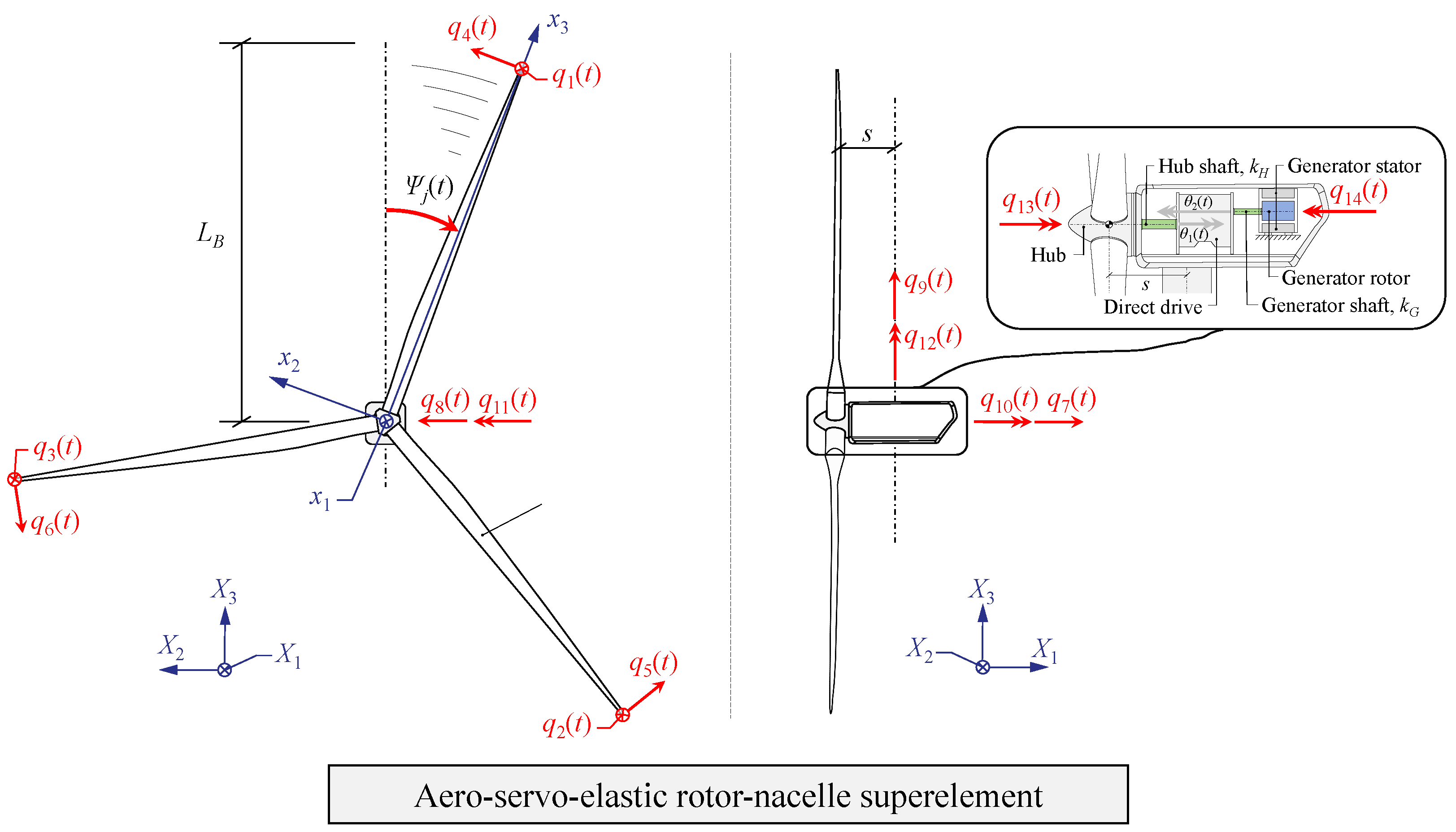
The rotor–nacelle superelement comprises three flexible blades, a hub, and a nacelle including the drivetrain system, with the corresponding physical model shown in Figure 1. To capture the primary wind–structure–controller interactions while ensuring consistent force and moment transfer across the substructure interface, the reduced-order rotor–nacelle model retains a baseline set of 14 DOFs. These include the first flapwise modal DOF $q_j$ and first edgewise modal DOF $q_{j+3}$ for blades $j=1,2,3$; the six rigid-body nacelle DOFs consisting of translational motions $q_7,q_8,q_9$ and rotational motions $q_{10},q_{11},q_{12}$; and the rotational deviation DOFs $q_{13}$ and $q_{14}$ associated with the rotor (hub) and generator shafts of the drivetrain. The DOFs of the blades and drivetrain shafts are defined within a local $x_1$-$x_2$-$x_3$ coordinate system (CS) that is fixed at the hub center and co-rotates with the rotor. As illustrated in Figure 1, the $x_1$-$x_2$ axes span the rotor plane, while the $x_3$-axis is normal to the plane. On the other hand, the translational and rotation DOFs governing the nacelle, i.e., $q_7,q_8,\dots ,q_{12}$, are resolved in the global inertial $X_1$-$X_2$-$X_3$ CS. The fore–aft motion is governed by $q_7$ (translation along the $X_1$-axis) and $q_{11}$ (rotation around the $X_2$-axis); the side–side motion is described by $q_8$ (translation along the $X_2$-axis) and $q_{10}$ (rotation around the $X_1$-axis); and the axial displacement and torsion correspond to $q_9$ and $q_{12}$ (translation along and rotation around the $X_3$-axis, respectively). The remaining DOFs, $q_{13}$ and $q_{14}$ describe the deviations of the hub and generator drivetrain shafts relative to their nominal azimuthal angles, respectively, encompassing potential rigid-body and torsional behaviors. The real-time azimuthal angles of the hub and generator shafts can then be expressed as ${\mathsf{\Omega }}_{0}t+q_{13}\left(t\right)$ and $N{\mathsf{\Omega }}_{0}t+q_{14}\left(t\right)$, respectively, where ${\mathsf{\Omega }}_0$ denotes the rated rotor speed and N is the gear ratio. Taking the time derivatives of these expressions yields the corresponding real-time rotor speed ${\mathsf{\Omega }}_r\left(t\right)$ and generator speed ${\mathsf{\Omega }}_g\left(t\right)$.

Within the framework of the modal formulation, the blade motion due to its elastic deformation is represented in the pitched local CS as a linear combination of the flapwise DOF $q_j$ and the edgewise DOF $q_{j+3}$ with their respective fundamental mode shapes ${\Phi }_f\left(x_3\right)$ and ${\Phi }_e\left(x_3\right)$. To evaluate the kinetic energy, this local deformation field needs to be transformed to the global CS via Euler angles. Accordingly, integrating the contributions of the nacelle rotations, the blade azimuth, and the blade pitch yields the global position field of the deformed blade j relative to the hub center:

$$\begin{array}{cc}\hfill {\mathbf{r}}_{B\leftarrow H,j}(x_3,t)& =\underset{{\mathbf{T}}_1}{\underbrace{\left[\begin{array}{ccc}1& 0& 0\\ 0& cos{q}_{10}& -sin{q}_{10}\\ 0& sin{q}_{10}& cos{q}_{10}\end{array}\right]}}\underset{{\mathbf{T}}_2}{\underbrace{\left[\begin{array}{ccc}cos{q}_{11}& 0& sin{q}_{11}\\ 0& 1& 0\\ -sin{q}_{11}& 0& cos{q}_{11}\end{array}\right]}}\underset{{\mathbf{T}}_3}{\underbrace{\left[\begin{array}{ccc}cos{q}_{12}& -sin{q}_{12}& 0\\ sin{q}_{12}& cos{q}_{12}& 0\\ 0& 0& 1\end{array}\right]}}\hfill \\ \hfill & \times \underset{{\mathbf{T}}_{{\Psi }_j}}{\underbrace{\left[\begin{array}{ccc}1& 0& 0\\ 0& cos{\Psi }_j& -sin{\Psi }_j\\ 0& sin{\Psi }_j& cos{\Psi }_j\end{array}\right]}}\underset{{\mathbf{T}}_{\beta }}{\underbrace{\left[\begin{array}{ccc}cos\beta & -sin\beta & 0\\ sin\beta & cos\beta & 0\\ 0& 0& 1\end{array}\right]}}\left(\begin{array}{c}{\Phi }_f\left(x_3\right)q_j\left(t\right)\\ {\Phi }_e\left(x_3\right)q_{j+3}\left(t\right)\\ x_3\end{array}\right)\hfill \end{array}$$

(1)

where ${\Psi }_j$ represents the azimuth angle of blade j, and $\beta$ denotes the collective pitch angle. ${\mathbf{T}}_1$,${\mathbf{T}}_2$,${\mathbf{T}}_3$,${\mathbf{T}}_{{\Psi }_j}$, and ${\mathbf{T}}_{\beta }$ are the local-to-global transformation matrices for the position vector. Treating the nacelle and hub as rigid bodies, their corresponding position vectors in global CS can also be obtained as:

$${\mathbf{r}}_N\left(t\right)=\left[\begin{array}{c}{q}_7\left(t\right)\\ q_8\left(t\right)\\ q_9\left(t\right)\end{array}\right],{\mathbf{r}}_{H\leftarrow N}\left(t\right)={\mathbf{T}}_1{\mathbf{T}}_2{\mathbf{T}}_3\left[\begin{array}{c}-s\\ 0\\ 0\end{array}\right]$$

(2)

where s is the overhang length of the hub. Summing ${\mathbf{r}}_N\left(t\right)$ and ${\mathbf{r}}_{H\leftarrow N}\left(t\right)$ in Equation (2) yields the global position vector of the hub, ${\mathbf{r}}_H\left(t\right)$, which is subsequently superimposed onto Equation (1) to determine the global position field of the deformed blade j, ${\mathbf{r}}_{B,j}(x_3,t)$ (It is worth noting that constant geometric parameters, such as tower-top length, shaft tilt, and rotor cone, can be straightforwardly integrated into these formulations). The translational structural velocity is determined by taking the time derivative of the position vector. Taking the global velocity field of the blade j, ${\mathbf{v}}_{B,j}(x_3,t)$, as an example, its first-order representation—after applying the small-angle approximation and truncating higher-order terms—is:

$$\begin{array}{c}\hfill {\mathbf{v}}_{B,j}(x_3,t)\simeq \left(\begin{array}{c}{\Phi }_f{\dot{q}}_{j}cos\beta +{\Phi }_e{\dot{q}}_{j+3}sin\beta +{\dot{q}}_7+{\dot{q}}_{11}{x}_{3}cos{\Psi }_j+{\dot{q}}_{12}{x}_{3}sin{\Psi }_j\\ -{\Phi }_f{\dot{q}}_{j}sin\beta +{\Phi }_e{\dot{q}}_{j+3}cos\beta +{\dot{q}}_{8}cos{\Psi }_j+{\dot{q}}_{9}sin{\Psi }_j-{\dot{q}}_{10}{x}_3+{\dot{q}}_{11}ssin{\Psi }_j-{\dot{q}}_{12}scos{\Psi }_j-x_3{\mathsf{\Omega }}_r\\ (-{\Phi }_f{q}_{j}sin\beta +{\Phi }_e{q}_{j+3}cos\beta ){\mathsf{\Omega }}_r-{\dot{q}}_{8}sin{\Psi }_j+{\dot{q}}_{9}cos{\Psi }_j+{\dot{q}}_{11}scos{\Psi }_j+{\dot{q}}_{12}ssin{\Psi }_j\end{array}\right)\end{array}$$

(3)

These approximations are adopted considering that the elastic blade deformation remains moderate relative to the blade span, for which such kinematic simplifications are commonly accepted in reduced-order global aeroelastic analyses of wind turbines. Meanwhile, the rotational velocities of these structural elements, including the nacelle rotation ${\omega }_N$, the hub rotation ${\omega }_H$, the generator rotor rotation ${\omega }_G$ and the blade-section rotation ${\omega }_{BS}$, expressed in their respective CSs are obtained as:

$$\begin{array}{cc}\hfill {\omega }_N\left(t\right)& =\left[\begin{array}{c}0\\ 0\\ {\dot{q}}_{12}\left(t\right)\end{array}\right]+{\mathbf{T}}_3^{\mathrm{T}}\left[\begin{array}{c}0\\ {\dot{q}}_{11}\left(t\right)\\ 0\end{array}\right]+{\left({\mathbf{T}}_2{\mathbf{T}}_3\right)}^{\mathrm{T}}\left[\begin{array}{c}{\dot{q}}_{10}\left(t\right)\\ 0\\ 0\end{array}\right],{\omega }_H\left(t\right)=\left[\begin{array}{c}{\mathsf{\Omega }}_r\left(t\right)+{\dot{q}}_{13}\left(t\right)\\ 0\\ 0\end{array}\right]+{\omega }_N\left(t\right),\hfill \\ \hfill {\omega }_G\left(t\right)& =\left[\begin{array}{c}-(N{\mathsf{\Omega }}_r\left(t\right)+{\dot{q}}_{14}\left(t\right))\\ 0\\ 0\end{array}\right],{\omega }_{BS}(x_3,t)={\left({\mathbf{T}}_{{\Psi }_j}{\mathbf{T}}_{\beta }\left[\begin{array}{ccc}cos{\theta }_a\left(x_3\right)& -sin{\theta }_a\left(x_3\right)& 0\\ sin{\theta }_a\left(x_3\right)& cos{\theta }_a\left(x_3\right)& 0\\ 0& 0& 1\end{array}\right]\right)}^{\mathrm{T}}{\omega }_H\left(t\right)\hfill \end{array}$$

(4)

where ${\theta }_a\left(x_3\right)$ is the aerodynamic pre-twist angle of the blade airfoil. The total kinetic energy and elastic potential energy of the system are formulated based on the derived position and velocity fields of the superelement. In particular, the elastic potential energy, associated with blade bending and shaft torsion, is calculated using Euler-Bernoulli beam theory and the Saint-Venant torsion rod model [34]. Substituting the calculated system energies into the Euler-Lagrange equations yields the equations of motion for the 14-DOF rotor–nacelle superelement:

$$\mathbf{M}\left(t\right)\ddot{\mathbf{q}}\left(t\right)+({\mathbf{C}}_s+\mathbf{G}\left(t\right))\dot{\mathbf{q}}\left(t\right)+\mathbf{K}\left(t\right)\mathbf{q}\left(t\right)={\mathbf{f}}_a\left(\dot{\mathbf{q}}\left(t\right),\mathbf{q}\left(t\right),\beta \left(t\right),t\right)+{\mathbf{f}}_g(\beta \left(t\right),t)+{\mathbf{f}}_{gen}\left(t\right)$$

(5)

On the left-hand side of Equation (5), $\mathbf{q}\left(t\right)={\{q_1,q_2,\dots ,q_{14}\}}^{\mathrm{T}}$ is the DOF vector for the superelement, and $\mathbf{M}\left(t\right)$, $\mathbf{G}\left(t\right)$, and $\mathbf{K}\left(t\right)$ represent the corresponding mass, gyroscopic, and stiffness matrices, respectively. The structural damping matrix ${\mathbf{C}}_s$ is formulated within a unified proportional damping framework. For the reduced-order components, damping is directly introduced in modal space, whereas a Rayleigh damping formulation is adopted for the FE tower–monopile substructure [35]. The Rayleigh coefficients are determined using the fundamental frequency and the first distinct higher mode whose frequency differs by more than 10%, thereby avoiding ill-conditioning associated with closely spaced symmetric modes. The gyroscopic matrix $\mathbf{G}\left(t\right)$ characterizes the velocity-dependent coupling arising from the Coriolis effect in spinning systems, a standard representation in rotating machinery dynamics [36]. To illustrate the coupling mechanisms among the structural components—namely the blades (B), nacelle (N), and drivetrain (D)—the system matrices (explicitly provided in the Supplementary Materials for a linear system) are partitioned into block form as follows:

$$\begin{array}{cc}\hfill \mathbf{M}\left(t\right)& =\left[\begin{array}{ccc}{\mathbf{M}}_{BB}& {\mathbf{M}}_{BN}\left(t\right)& {\mathbf{M}}_{BD}\left(t\right)\\ {\mathbf{M}}_{BN}^T\left(t\right)& {\mathbf{M}}_{NN}\left(t\right)& {\mathbf{M}}_{ND}\left(t\right)\\ {\mathbf{M}}_{BD}^T\left(t\right)& {\mathbf{M}}_{ND}^T\left(t\right)& {\mathbf{M}}_{DD}\left(t\right)\end{array}\right],\hfill \\ \hfill \mathbf{G}\left(t\right)& =\left[\begin{array}{ccc}{\mathbf{0}}_{6\times 6}& {\mathbf{G}}_{BN}\left(t\right)& {\mathbf{0}}_{6\times 2}\\ {\mathbf{G}}_{NB}\left(t\right)& {\mathbf{G}}_{NN}\left(t\right)& {\mathbf{0}}_{6\times 2}\\ {\mathbf{0}}_{2\times 6}& {\mathbf{0}}_{2\times 6}& {\mathbf{0}}_{2\times 2}\end{array}\right],\mathbf{K}\left(t\right)=\left[\begin{array}{ccc}{\mathbf{K}}_{BB}\left(t\right)& {\mathbf{0}}_{6\times 6}& {\mathbf{0}}_{6\times 2}\\ {\mathbf{K}}_{NB}\left(t\right)& {\mathbf{0}}_{6\times 6}& {\mathbf{0}}_{6\times 2}\\ {\mathbf{0}}_{2\times 6}& {\mathbf{0}}_{2\times 6}& {\mathbf{K}}_{DD}\end{array}\right]\hfill \end{array}$$

(6)

where, among the nonzero submatrices, only the blade-related mass submatrix ${\mathbf{M}}_{BB}$ and the drivetrain-related stiffness submatrix ${\mathbf{K}}_{DD}$ are constant, while all others exhibit time dependence due to blade pitch variation and rotor rotation. As a representative example, the elements of the gyroscopic submatrix ${\mathbf{G}}_{BN}\left(t\right)$ corresponding to the blade j are expressed as:

$$\begin{array}{cccc}\hfill g_{j,11}& =-2{\mathsf{\Omega }}_{r}sin{\Psi }_{j}cos\beta M_f,\hfill & \hfill g_{j+3,11}& =-2{\mathsf{\Omega }}_{r}sin{\Psi }_{j}sin\beta M_e\hfill \\ \hfill g_{j,12}& =2{\mathsf{\Omega }}_{r}cos{\Psi }_{j}cos\beta M_f,\hfill & \hfill g_{j+3,12}& =2{\mathsf{\Omega }}_{r}cos{\Psi }_{j}sin\beta M_e\hfill \end{array}$$

(7)

where the modal mass moments, $M_f$ and $M_e$, are defined as ${\displaystyle M_{f/e}={\int }_0^{L_b}{x}_3{\mu }_b\left(x_3\right){\Phi }_{f/e}\left(x_3\right)d{x}_3}$. The coupling terms in Equation (7), proportional to the rotor rotational speed of ${\mathsf{\Omega }}_r$, appear in the orthogonal generalized coordinates $q_{11}$ and $q_{12}$ (Figure 1), thereby representing the gyroscopic coupling within the superelement. These terms also exhibit an explicit trigonometric dependence on the blade pitch angle $\beta$. Consequently, under below-rated operating conditions ($\beta =0$), the gyroscopic coupling inherent in the submatrix ${\mathbf{G}}_{BN}\left(t\right)$ manifests exclusively in the terms related to the blade flapwise vibration. Furthermore, the off-diagonal submatrices in Equation (6) characterize the coupling interactions among different subsystems arising from inertial, gyroscopic, and elastic effects. In particular, ${\mathbf{M}}_{BN}\left(t\right)$, ${\mathbf{M}}_{BD}\left(t\right)$, and ${\mathbf{M}}_{ND}\left(t\right)$ describe the inertial couplings between the blade–nacelle, blade–drivetrain, and nacelle–drivetrain subsystems, respectively. The gyroscopic coupling between the blades and nacelle, primarily governed by rotor rotation, is described by ${\mathbf{G}}_{BN}\left(t\right)$ and ${\mathbf{G}}_{NB}\left(t\right)$, while the corresponding elastic coupling is represented by ${\mathbf{K}}_{BN}(={\mathbf{0}}_{6\times 6})$ and ${\mathbf{K}}_{NB}\left(t\right)$. The asymmetry of the gyroscopic and stiffness matrices, $\mathbf{G}\left(t\right)$ and $\mathbf{K}\left(t\right)$, reflects the cross-coupled and direction-dependent dynamics within the superelement. On the right-hand side of Equation (5), ${\mathbf{f}}_a(\dot{\mathbf{q}}\left(t\right),\mathbf{q}\left(t\right),\beta \left(t\right),t)$ is the nonlinear aerodynamic load vector, while ${\mathbf{f}}_g(\beta \left(t\right),t)$ and ${\mathbf{f}}_{gen}\left(t\right)$ represent the gravity and generator load vectors, respectively, all of which are modeled in the following sections.

2.2. Aerodynamic Load Modeling

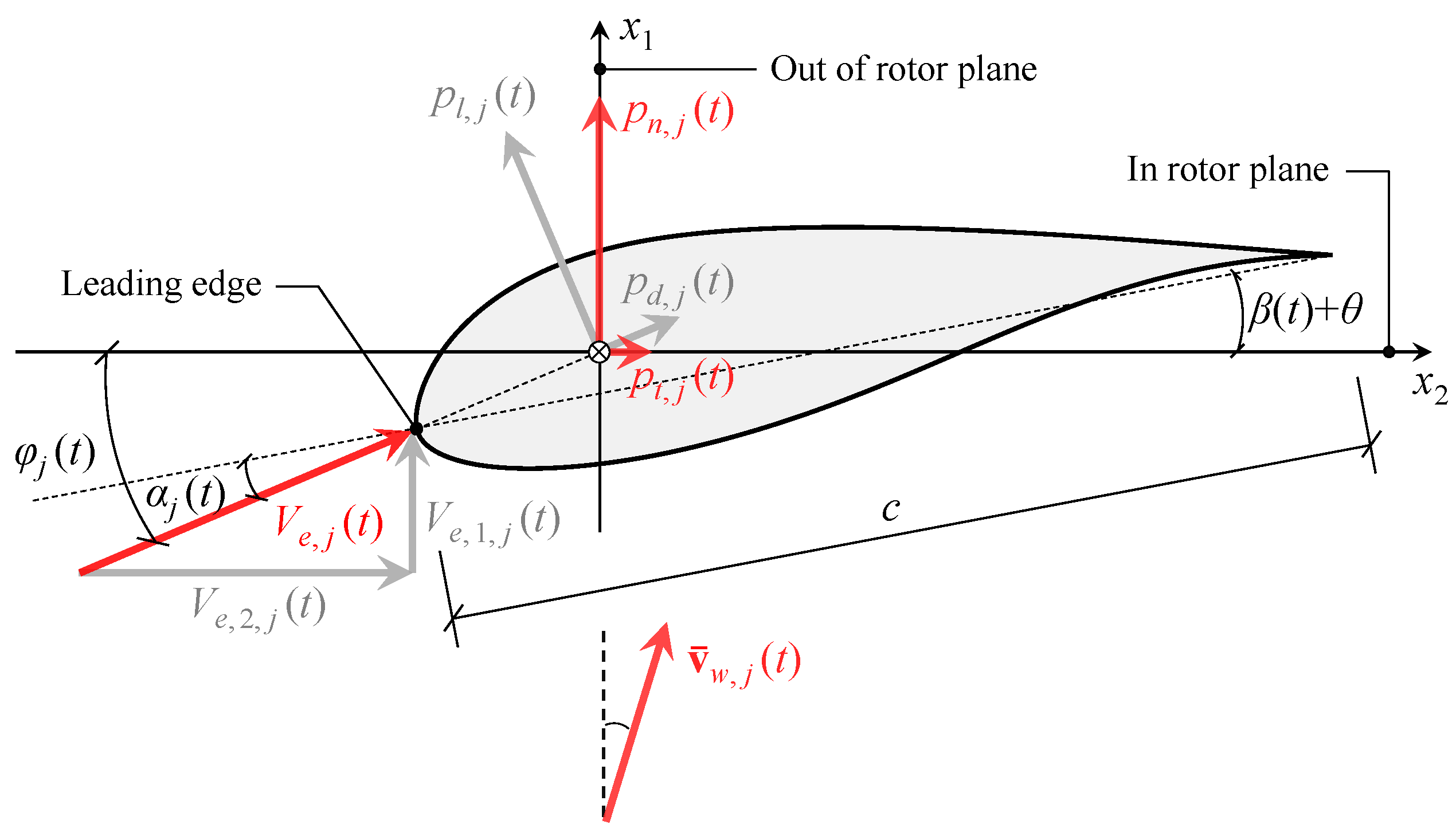
The aerodynamic loads on the blades are evaluated based on a modified BEM framework, incorporating Prandtl’s tip loss correction and Glauert’s turbulence wake correction [37]. Specifically, the distributed aerodynamic forces per unit length for each airfoil on the blade are determined first, followed by the formulation of the modal aerodynamic loads using the principle of virtual work. As shown in Figure 2, the aerodynamic analysis is conducted for an airfoil section at a radial distance $x_3$ from the hub center on blade j.

Given the undisturbed mean wind velocity ${\overline{\mathbf{v}}}_{w,j}(x_3,t)$ (already projected into the local blade CS), the normal and tangential components of effective wind velocity ${\mathbf{v}}_{e,j}(x_3,t)$ relative to the rotor plane is expressed as:

$$\left(\begin{array}{c}{V}_{e,1,j}(x_3,t)\\ V_{e,2,j}(x_3,t)\end{array}\right)=\underset{\mathrm{Mean}\mathrm{wind}\mathrm{velocity}\mathrm{with}\mathrm{induction}}{\underbrace{\left[\begin{array}{cc}1-a_j& 0\\ 0& 1+a_j^{\prime }\end{array}\right]\left(\begin{array}{c}{\overline{V}}_{w,1,j}\\ {\overline{V}}_{w,2,j}+x_3{\mathsf{\Omega }}_r\end{array}\right)}}+\underset{\mathrm{Turbulence}}{\underbrace{\left(\begin{array}{c}{\upsilon }_{1,j}^{\prime }\\ {\upsilon }_{2,j}^{\prime }\end{array}\right)}}-\underset{\mathrm{Blade}\mathrm{vibration}}{\underbrace{\left(\begin{array}{c}{V}_{B,1,j}\\ V_{B,2,j}+x_3{\mathsf{\Omega }}_r\end{array}\right)}}$$

(8)

where the two components of ${\mathbf{v}}_{e,j}(x_3,t)$, ${\overline{V}}_{e,1,j}(x_3,t)$ and ${\overline{V}}_{e,2,j}(x_3,t)$, are aligned with the local $x_1$- and $x_2$-axes, respectively. In a similar manner, ${\overline{V}}_{w,1,j}(x_3,t)$ and ${\overline{V}}_{w,2,j}(x_3,t)$ are the first two axial components of ${\overline{\mathbf{v}}}_{w,j}(x_3,t)$. $V_{B,1,j}(x_3,t)$ and $V_{B,2,j}(x_3,t)$ are the first two elements of the blade velocity ${\mathbf{v}}_{B,j}(x_3,t)$ expressed in Equation (3). Removing the rotor-speed-induced term $x_3{\mathsf{\Omega }}_r\left(t\right)$ from the tangential component $V_{B,2,j}(x_3,t)$ yields the blade vibrational velocity, which gives rise to the portion of the aerodynamic loads dependent on the structural velocity $\dot{\mathbf{q}}\left(t\right)$, thereby establishing the aeroelastic coupling within the system. ${\upsilon }_{1,j}^{\prime }(x_3,t)$ and ${\upsilon }_{2,j}^{\prime }(x_3,t)$ correspond to the normal and tangential components of the turbulence, which have zero mean and exhibit stochastic variability. The induced wind velocity, quantified by the induction factors $a_j(x_3,t)$ and $a_j^{\prime }(x_3,t)$, develops as the undisturbed flow passes through the rotor disk region. According to the modified BEM theory, these induction factors are determined iteratively following the procedure detailed in [37]. Convergence is achieved when the maximum absolute change in the induced velocity components between successive iterations falls below 0.01 m/s. The maximum number of iterations is limited to 100 to maintain numerical robustness under strongly nonlinear aerodynamic conditions. Furthermore, referring to Figure 2, the inflow angle ${\phi }_j(x_3,t)$ can be calculated via Equation (8), which further yields the angle of attack as ${\alpha }_j(x_3,t)={\phi }_j(x_3,t)-{\theta }_a\left(x_3\right)-\beta \left(t\right)$. The normal and tangential aerodynamic forces on blade j per unit length are then computed as:

$$\begin{array}{cc}\hfill \left(\begin{array}{c}{p}_{n,j}(x_3,t)\\ p_{t,j}(x_3,t)\end{array}\right)& =\left[\begin{array}{cc}cos{\phi }_j& sin{\phi }_j\\ -sin{\phi }_j& cos{\phi }_j\end{array}\right]\left(\begin{array}{c}{p}_{l,j}\\ p_{d,j}\end{array}\right)={\displaystyle \frac{1}{2}}\rho V_{e,j}^{2}c\left[\begin{array}{cc}cos{\phi }_j& sin{\phi }_j\\ -sin{\phi }_j& cos{\phi }_j\end{array}\right]\left(\begin{array}{c}{c}_l\left({\alpha }_j\right)\\ c_d\left({\alpha }_j\right)\end{array}\right)\hfill \end{array}$$

(9)

where the aerodynamic lift $p_{l,j}(x_3,t)$ and drag $p_{d,j}(x_3,t)$, the resultant effective wind speed $V_{e,j}(x_3,t)$, and the airfoil chord length $c\left(x_3\right)$ are illustrated in Figure 2. $\rho$ denotes the air density, and $c_l\left({\alpha }_j\right)$ and $c_d\left({\alpha }_j\right)$ are the lift and drag coefficients of a given airfoil. Utilizing the principle of virtual work, the elements of the modal aerodynamic load vector ${\mathbf{f}}_a\left(\dot{\mathbf{q}}\left(t\right),\mathbf{q}\left(t\right),\beta \left(t\right),t\right)$ are derived by integrating the distributed aerodynamic forces over the blade length $L_B$ as follows:

$$\begin{array}{cc}\hfill & f_{a,j}\left(t\right)={\int }_0^{L_B}{\Phi }_f^T\left(p_{n,j}(x_3,t)cos\beta -p_{t,j}(x_3,t)sin\beta \right)\mathrm{d}{x}_3,j=1,2,3\hfill \end{array}$$

(10)

$$\begin{array}{cc}\hfill & f_{a,j+3}\left(t\right)={\int }_0^{L_B}{\Phi }_e^T\left(p_{n,j}(x_3,t)sin\beta +p_{t,j}(x_3,t)cos\beta \right)\mathrm{d}{x}_3,\hfill \end{array}$$

(11)

$$\begin{array}{cc}\hfill & f_{a,7}\left(t\right)={\displaystyle \sum _{j=1}^3}{\int }_0^{L_B}{p}_{n,j}(x_3,t)\mathrm{d}{x}_3,\hfill \end{array}$$

(12)

$$\begin{array}{cc}\hfill & f_{a,8}\left(t\right)={\displaystyle \sum _{j=1}^3}{\int }_0^{L_B}{p}_{t,j}(x_3,t)cos{\Psi }_j\mathrm{d}{x}_3,\hfill \end{array}$$

(13)

$$\begin{array}{cc}\hfill & f_{a,9}\left(t\right)={\displaystyle \sum _{j=1}^3}{\int }_0^{L_B}{p}_{t,j}(x_3,t)sin{\Psi }_j\mathrm{d}{x}_3,\hfill \end{array}$$

(14)

$$\begin{array}{cc}\hfill & f_{a,10}\left(t\right)=-{\displaystyle \sum _{j=1}^3}{\int }_0^{L_B}{x}_3·p_{t,j}(x_3,t)\mathrm{d}{x}_3,\hfill \end{array}$$

(15)

$$\begin{array}{cc}\hfill & f_{a,11}\left(t\right)={\displaystyle \sum _{j=1}^3}{\int }_0^{L_B}{x}_3·p_{n,j}(x_3,t)cos{\Psi }_j\mathrm{d}{x}_3+{\displaystyle \sum _{j=1}^3}{\int }_0^{L_B}s·p_{t,j}(x_3,t)sin{\Psi }_j\mathrm{d}{x}_3,\hfill \end{array}$$

(16)

$$\begin{array}{cc}\hfill & f_{a,12}\left(t\right)={\displaystyle \sum _{j=1}^3}{\int }_0^{L_B}{x}_3·p_{n,j}(x_3,t)sin{\Psi }_j\mathrm{d}{x}_3-{\displaystyle \sum _{j=1}^3}{\int }_0^{L_B}s·p_{t,j}(x_3,t)cos{\Psi }_j\mathrm{d}{x}_3,\hfill \end{array}$$

(17)

$$\begin{array}{cc}\hfill & f_{a,13}\left(t\right)=-(1-\mu ){\displaystyle \sum _{j=1}^3}{\int }_0^{L_B}{x}_3·p_{t,j}(x_3,t)\mathrm{d}{x}_3.\hfill \end{array}$$

(18)

where $\mu$ is the friction coefficient of the drivetrain. Specifically, $f_{a,1}\left(t\right)$ to $f_{a,6}\left(t\right)$ represent the generalized modal aerodynamic loads on the blade flapwise and edgewise DOFs, $q_1\left(t\right)$ to $q_6\left(t\right)$, while $f_{a,7}\left(t\right)$ to $f_{a,12}\left(t\right)$ correspond to the nacelle DOFs, $q_7\left(t\right)$ to $q_{12}\left(t\right)$. In the absence of modal aerodynamic loads on the generator DOF $q_{14}\left(t\right)$, the associated 14th element of ${\mathbf{f}}_a(\dot{\mathbf{q}}\left(t\right),\mathbf{q}\left(t\right),\beta \left(t\right),t)$, denoted as $f_{a,14}$, is zero.

2.3. Gravitational Load and Servo Control Modeling

Within the 14-DOF aeroelastic model, the gravitational effects exerted on the three blades along the $x_1$- and $x_2$-axes are taken into consideration. The expression for the corresponding modal gravitational load, ${\mathbf{f}}_g(\beta \left(t\right),t)$, is defined as follows:

$$\begin{array}{cc}\hfill {\mathbf{f}}_g(\beta \left(t\right),t)& =g\{m_{f}sin{\Psi }_1\left(t\right)sin\beta \left(t\right)m_{f}sin{\Psi }_2\left(t\right)sin\beta \left(t\right)m_{f}sin{\Psi }_3\left(t\right)sin\beta \left(t\right)\hfill \\ \hfill & -m_{e}sin{\Psi }_1\left(t\right)cos\beta \left(t\right)-m_{e}sin{\Psi }_2\left(t\right)cos\beta \left(t\right)-m_{e}sin{\Psi }_3\left(t\right)cos\beta \left(t\right){\mathbf{0}}_{8\times 1}{\}}^{\mathrm{T}}\hfill \end{array}$$

(19)

Here, the parameters $m_f$ and $m_e$ represent the respective modal masses of the blade in the flapwise and edgewise directions, while g stands for the gravitational acceleration constant.

The system’s servo control, which integrates both collective pitch control and generator torque control, is established using a gain-scheduled PI algorithm combined with a first-order low-pass filter [38,39,40]. Once the mean wind speed goes beyond its rated value, the collective pitch control engages ($\beta \left(t\right)>0$). The primary objective here is to maintain the generator speed at its rated level, denoted by $N{\mathsf{\Omega }}_0$. Consequently, the formulation for the pitch control signal at a specific time step $t_m$ is given by:

$$\beta \left(t_m\right)=K_{pr}e\left(t_m\right)+K_{in}{\displaystyle \sum _{n=0}^m}e\left(t_n\right)·(t_n-t_{n-1})$$

(20)

In this equation, the generator speed error is expressed as $e\left(t_m\right)=N{\mathsf{\Omega }}_0-{\mathsf{\Omega }}_{Ge{n}_f}\left(t_m\right)$, where ${\mathsf{\Omega }}_{Ge{n}_f}\left(t_m\right)$ refers to the filtered real-time generator speed. The dynamic scheduling of the proportional and integral gains ($K_{pr}$ and $K_{in}$) is dependent on the filtered pitch angle ${\beta }_f\left(t_m\right)$. For the numerical case study presented later, the determination of these gains relies on the scheduling strategy originally designed for the reference 10 MW OWT, as described in [41]. Regarding the control of generator torque ${\mathbf{f}}_{gen}\left(t\right)$, a fine-tuned ROSCO controller algorithm is adopted [42]. This controller operation is divided into four distinct regions: Regions 1/1.5, 2, 2.5, and 3. Operating as transition zones, Regions 1/1.5 and 2.5 utilize PI controllers to achieve specific targets: attaining the minimum generator speed and the rated generator speed, respectively. The primary function of Region 2 is to maximize power extraction through optimal tip-speed ratio tracking when the wind speed is below the rated value. In contrast, when the wind speed surpasses its rated threshold, Region 3 is tasked with maintaining a constant generator torque. Furthermore, to mitigate high-frequency oscillations, the generator torque controller relies on a filtered generator speed signal for its input.

3. Coupling and Verification of the Rotor–Nacelle Superelement

This section presents and validates the hybrid modeling framework of the fully coupled OWT system using the aero–servo–elastic rotor–nacelle superelement developed in Section 2. Section 3.1 formulates a 3-DOF modal-based tower–monopile substructure represented by an idealized continuous beam with a clamped-base boundary condition. This configuration—explicitly omitting soil–structure interactions and local joint flexibility—is chosen to maintain modeling consistency with the modal-based OpenFAST benchmark and to provide a baseline configuration for verification of the proposed coupling framework. This simplified substructure enables direct comparison with OpenFAST prior to the introduction of the high-fidelity FE substructure in Section 4. Section 3.2 and Section 3.3 present the system assembly procedure and the corresponding time-domain verification results.

3.1. Hydroelastic Tower–Monopile Substructure

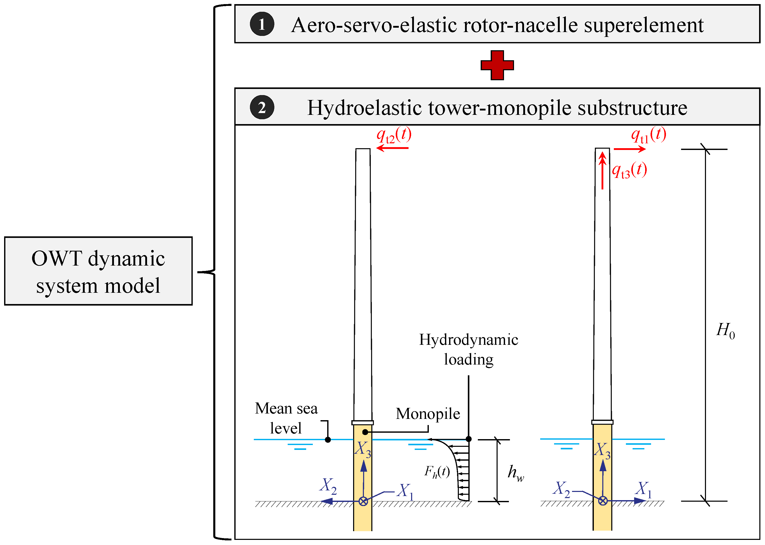
As shown in Figure 3, in order to incorporate the aero–servo–elastic rotor–nacelle superelement into the OWT system dynamics, a hydroelastic model of the tower–monopile substructure is required. Within the modal-based framework, the tower and monopile are treated as a unified substructure, where the dominant low-frequency dynamics are represented by the fore–aft DOF $q_{t1}$, the side–side DOF $q_{t2}$, and the torsional DOF $q_{t3}$.

The associated fundamental mode shapes in the fore–aft, side–side, and torsional directions are denoted by ${\Phi }_{t1}\left(X_3\right)$, ${\Phi }_{t2}\left(X_3\right)$, and ${\Phi }_{t3}\left(X_3\right)$, respectively. Following the similar methodology used in Section 2 for the modeling of the rotor–nacelle superelement, the governing equations of motion for the tower–monopile substructure are derived as:

$${\mathbf{M}}_t{\ddot{\mathbf{q}}}_t\left(t\right)+{\mathbf{C}}_t{\dot{\mathbf{q}}}_t\left(t\right)+{\mathbf{K}}_t{\mathbf{q}}_t\left(t\right)={\mathbf{f}}_h\left({\ddot{\mathbf{q}}}_t\left(t\right),{\dot{\mathbf{q}}}_t\left(t\right),t\right)$$

(21)

where ${\mathbf{q}}_t\left(t\right)={\{q_{t1},q_{t2},q_{t3}\}}^{\top }$ is the DOF vector for the substructure, while ${\mathbf{M}}_t$, ${\mathbf{C}}_t$, and ${\mathbf{K}}_t$ denote the corresponding mass, damping, and stiffness matrices. The mass and stiffness matrices in Equation (21) are provided as:

$${\mathbf{M}}_t={\int }_0^{H_0}\left[\begin{array}{ccc}{\Phi }_{t1}^2{m}_t+J_t{\Phi }_{t1}^{\prime 2}& 0& 0\\ 0& {\Phi }_{t2}^2{m}_t+J_t{\Phi }_{t2}^{\prime 2}& 0\\ 0& 0& 2J_t{\Phi }_{t3}^2\end{array}\right]\mathrm{d}{X}_3,{\mathbf{K}}_t={\int }_0^{H_0}\left[\begin{array}{ccc}E{I}_t{\Phi }_{t1}^{\prime \prime 2}& 0& 0\\ 0& E{I}_t{\Phi }_{t2}^{\prime \prime 2}& 0\\ 0& 0& G{J}_t{\Phi }_{t3}^{\prime 2}\end{array}\right]\mathrm{d}{X}_3$$

(22)

where ${\Phi }_{tk}^{\prime }\left(X_3\right)$ and ${\Phi }_{tk}^{\prime \prime }\left(X_3\right)$ for $k=1,2,3$ denote the first and second derivatives of the substructure’s mode shape ${\Phi }_{tk}\left(X_3\right)$ with respect to the height $X_3$. The terms $m_t\left(X_3\right)$, $I_t\left(X_3\right)$, and $J_t\left(X_3\right)$ represent the distributed mass, area moment of inertia, and polar moment of inertia of the substructure’s circular section, respectively. $E\left(X_3\right)$ and $G\left(X_3\right)$ are the elastic and shear moduli of the material. Additionally, the integrals corresponding to the diagonal matrix entries are evaluated over the interval $[0,H_0]$, where $H_0$ denotes the tower height above the seabed. The structural damping matrix ${\mathbf{C}}_t$ is constructed using prescribed modal damping ratios in conjunction with Rayleigh’s formulation.

To determine the hydrodynamic load ${\mathbf{f}}_h\left({\ddot{\mathbf{q}}}_t\left(t\right),{\dot{\mathbf{q}}}_t\left(t\right),t\right)$ on the left side of Equation (21), this study applies Morison’s equation [43], which effectively characterizes the fluid–structure interaction between the submerged portion of the monopile and the steady water or incoming waves. For cylindrical support structures, the elemental hydrodynamic force is calculated as the superposition of three distinct terms:

$$d{F}_h=\underset{\mathrm{Froude}–\mathrm{Krylov}\mathrm{force}}{\underbrace{{\rho }_w{\displaystyle \frac{\pi D^2}{4}}\mathrm{d}{X}_3{\ddot{u}}_w}}+\underset{\mathrm{Hydrodynamic}\mathrm{mass}\mathrm{force}}{\underbrace{{\rho }_w{C}_A{\displaystyle \frac{\pi D^2}{4}}\mathrm{d}{X}_3({\ddot{u}}_w-{\ddot{u}}_s)}}+\underset{\mathrm{Drag}\mathrm{force}}{\underbrace{{\displaystyle \frac{1}{2}}{\rho }_w{C}_{D}D\mathrm{d}{X}_3({\dot{u}}_w-{\dot{u}}_s)|{\dot{u}}_w-{\dot{u}}_s|}}$$

(23)

where ${\rho }_w$ and D refer to the density of water and the outer diameter of the monopile, respectively. The drag coefficient $C_D$ and the added mass coefficient $C_A$ are empirically determined values, both taken as 1.0 for cylindrical shapes [44]. Moreover, the structural kinematics are defined by the velocity ${\dot{u}}_s$ and acceleration ${\ddot{u}}_s$, while the horizontal fluid velocity and acceleration are denoted as ${\dot{u}}_w$ and ${\ddot{u}}_w$, respectively. By applying the principle of virtual work, the non-zero elements of the modal hydrodynamic load ${\mathbf{f}}_h\left({\ddot{\mathbf{q}}}_t\left(t\right),{\dot{\mathbf{q}}}_t\left(t\right),t\right)$, associated with the fore–aft $q_{t1}\left(t\right)$ and side–side $q_{t2}\left(t\right)$ DOFs, are obtained by multiplying Equation (23) with their respective mode shapes, ${\Phi }_{t1}\left(X_3\right)$ and ${\Phi }_{t2}\left(X_3\right)$, and integrating along the submerged portion of the monopile.

3.2. Fully Coupled Aero-Hydro-Servo-Elastic OWT System

In essence, the analytical model of the fully coupled OWT system is established by combining the governing equations of the 14-DOF superelement (Equation (5)) with those of the substructure, as illustrated in Figure 3. For the 3-DOF tower–monopile model developed in Section 3.1, this combination corresponds to the coupling of Equations (5) and (21). Furthermore, owing to the rigid connection at the tower–nacelle interface and the consistent definition of the CS, the substructure DOFs $q_{t1}\left(t\right)$, $q_{t2}\left(t\right)$, $q_{t3}\left(t\right)$ are directly compatible with the superelement DOFs $q_7\left(t\right)$, $q_8\left(t\right)$, $q_{12}\left(t\right)$, respectively, allowing them to be used interchangeably in the governing equations. To finalize the system setup, the DOF $q_9\left(t\right)$ is eliminated since the axial deformation of the substructure is neglected in the present modal-based OWT model. Meanwhile, the adoption of Euler–Bernoulli beam theory imposes a kinematic constraint, meaning that the nacelle rotation DOFs, $q_{10}\left(t\right)$ and $q_{11}\left(t\right)$, are no longer independent variables. Instead, they are analytically derived from the substructure bending DOFs, $q_7\left(t\right)$ and $q_8\left(t\right)$, in conjunction with their corresponding mode shape values at the tower top, given as [18]:

$$q_{10}\left(t\right)=-q_8\left(t\right){\Phi }_{t2}^{\prime }\left(H_0\right),q_{11}\left(t\right)=q_7\left(t\right){\Phi }_{t1}^{\prime }\left(H_0\right)$$

(24)

Consequently, the combination of Equations (5) and (21) yields the governing equations of an 11-DOF fully coupled system:

$$\tilde{\mathbf{M}}\left(t\right)\ddot{\tilde{\mathbf{q}}}\left(t\right)+\tilde{\mathbf{C}}\left(t\right)\dot{\tilde{\mathbf{q}}}\left(t\right)+\tilde{\mathbf{K}}\left(t\right)\tilde{\mathbf{q}}\left(t\right)={\tilde{\mathbf{f}}}_a\left(\dot{\tilde{\mathbf{q}}}\left(t\right),\tilde{\mathbf{q}}\left(t\right),\beta \left(t\right),t\right)+{\tilde{\mathbf{f}}}_h\left(\ddot{\tilde{\mathbf{q}}}\left(t\right),\dot{\tilde{\mathbf{q}}}\left(t\right),t\right)+{\tilde{\mathbf{f}}}_g(\beta \left(t\right),t)+{\tilde{\mathbf{f}}}_{gen}\left(t\right)$$

(25)

where $\tilde{\mathbf{q}}\left(t\right)={\{q_1,q_2,\dots ,q_8,q_{12},q_{13},q_{14}\}}^{\mathrm{T}}$ is the DOF vector of the coupled system, and $\tilde{\mathbf{M}}\left(t\right)$, $\tilde{\mathbf{C}}\left(t\right)$, and $\tilde{\mathbf{K}}\left(t\right)$ are the associated mass, damping and gyroscopic, and stiffness matrices. These system matrices are obtained through the same subsystem coupling procedure and are provided in the Supplementary Materials. Taking the mass matrix $\tilde{\mathbf{M}}\left(t\right)$ as an example, its expression, derived by superimposing the subsystem mass matrices from Equations (6) and (22) onto their shared DOFs, is given by:

$$\begin{array}{cc}\hfill \tilde{\mathbf{M}}\left(t\right)& =\left[\begin{array}{ccc}{\mathbf{M}}_{BB}& {\mathbf{M}}_{BT}\left(t\right)& {\mathbf{M}}_{BD}\left(t\right)\\ {\mathbf{M}}_{BT}^T\left(t\right)& {\mathbf{M}}_{TT}\left(t\right)& {\mathbf{M}}_{TD}\left(t\right)\\ {\mathbf{M}}_{BD}^T\left(t\right)& {\mathbf{M}}_{TD}^T\left(t\right)& {\mathbf{M}}_{DD}\left(t\right)\end{array}\right],\hfill \end{array}$$

(26)

where the submatrices ${\mathbf{M}}_{BB}$, ${\mathbf{M}}_{BD}\left(t\right)$, and ${\mathbf{M}}_{DD}\left(t\right)$ pertain solely to the blade and drivetrain, allowing them to be directly adopted from Equation (6). In contrast, the $3\times 3$ submatrices related to the substructure—namely ${\mathbf{M}}_{BT}\left(t\right)$, ${\mathbf{M}}_{TT}\left(t\right)$, and ${\mathbf{M}}_{TD}\left(t\right)$—are derived by applying the two above-mentioned DOF elimination procedures to the $6\times 6$ submatrices ${\mathbf{M}}_{BN}\left(t\right)$, ${\mathbf{M}}_{NN}\left(t\right)$, and ${\mathbf{M}}_{ND}\left(t\right)$ from Equation (6), and subsequently superimposing them with the $3\times 3$ matrix ${\mathbf{M}}_t$ from Equation (22).

Correspondingly, the right-hand side of Equation (25) comprises the $11\times 1$ external modal load vectors of the fully coupled OWT system. The original hydrodynamic load vector ${\mathbf{f}}_h\left({\ddot{\mathbf{q}}}_t\left(t\right),{\dot{\mathbf{q}}}_t\left(t\right),t\right)$ (Equation (21)), gravitational load vector ${\mathbf{f}}_g(\beta \left(t\right),t)$ (Equation (19)), and generator torque vector ${\mathbf{f}}_{gen}\left(t\right)$ (Equation (5)) do not directly act on the eliminated dependent DOFs $q_{10}\left(t\right)$ and $q_{11}\left(t\right)$. Therefore, they simply need to be zero-padded at the indices of the missing DOFs to form their system-level representations, denoted by the tilde (∼) in Equation (25). However, the aerodynamic loads acting on the originally dependent nacelle rotation DOFs, $q_{10}\left(t\right)$ and $q_{11}\left(t\right)$, as expressed in Equations (15) and (16), must be projected onto their corresponding master substructure bending DOFs, $q_8\left(t\right)$ and $q_7\left(t\right)$, respectively. Applying the principle of virtual work, the updated aerodynamic load terms for the fore–aft and side–side directions, $f_{a,7}\left(t\right)$ and $f_{a,8}\left(t\right)$, are expressed as follows:

$$\begin{array}{cc}\hfill & f_{a,7}\left(t\right)={\displaystyle \sum _{j=1}^3}{\int }_0^{L_B}{p}_{n,j}(x_3,t)\mathrm{d}{x}_3+{\Phi }_{t1}^{\prime }\left(H_0\right)({\displaystyle \sum _{j=1}^3}{\int }_0^{L_B}{x}_3·p_{n,j}(x_3,t)cos{\Psi }_j\mathrm{d}{x}_3\hfill \end{array}$$

$$\begin{array}{cc}\hfill & +{\displaystyle \sum _{j=1}^3}{\int }_0^{L_B}s·p_{t,j}(x_3,t)sin{\Psi }_j\mathrm{d}{x}_3),\hfill \end{array}$$

(27)

$$\begin{array}{cc}\hfill & f_{a,8}\left(t\right)={\displaystyle \sum _{j=1}^3}{\int }_0^{L_B}{p}_{t,j}(x_3,t)cos{\Psi }_j\mathrm{d}{x}_3+{\Phi }_{t2}^{\prime }\left(H_0\right){\displaystyle \sum _{j=1}^3}{\int }_0^{L_B}{x}_3·p_{t,j}(x_3,t)\mathrm{d}{x}_3.\hfill \end{array}$$

(28)

Importantly, the fully coupled OWT model synthesized by assembling the matrices and external load vectors of the above superelement and substructure models is mathematically equivalent to the OWT model constructed integrally using modal-based and multibody dynamics formulations [24]. This equivalence is fundamentally rooted in the additive property of kinetic and potential energies, enabling the governing equations of system dynamics to be derived either globally or separately. As a result, the proposed aero–servo–elastic superelement fully preserves its structural and aeroelastic coupling with the substructure via the six spatial DOFs of the nacelle, providing the theoretical foundation that integrating this superelement with substructure models—whether in system hybrid formulation, co-simulations, or real-time hybrid simulations—is capable of accurately reproducing comprehensive dynamics of the OWT system.

3.3. Time-Domain Verification Against OpenFAST

To verify the accuracy of the 11-DOF fully coupled system model based on the aero–servo–elastic superelement, its time-domain responses are compared with those obtained from the widely used aeroelastic simulation tool OpenFAST (v4.0.4). The structural and aerodynamic data originate from the IEA 10 MW monopile-supported OWT [41], designed for a water depth of 30 m. Its key geometric and operational parameters are detailed in

Table 1. Key parameters of the IEA 10-MW monopile supported offshore wind turbine [41].

Rated Power	10.0 MW (IEC Class 1A)
Rotor orientation, configuration	Upwind, 3 blades
Control	Variable speed, collective pitch
Drivetrain	Direct-drive gearbox
Rated, cut-in rotor speed	8.7 rpm, 5.0 rpm
Rated, cut-in, cut-out wind speed	10.7 m/s, 4 m/s, 25 m/s
Rotor, hub diameter	198.3 m, 4.6 m
Overhang	7.1 m
Tower top height above the mean sea level	115.6 m

.

To ensure maximum physical consistency, the OpenFAST model is tailored to include the first flapwise and edgewise bending modes of the blades, the first fore–aft and side–side bending modes of the tower–monopile substructure, as well as the drivetrain torsional flexibility and generator DOFs. Unsteady aerodynamic effects, including dynamic inflow and dynamic stall, are disabled, and higher-order geometric features such as rotor cone and shaft tilt are neglected (set to zero). The validation load case adopts a typical offshore wind shear exponent of 0.1 and an above-rated mean hub-height wind speed of 17 m/s.

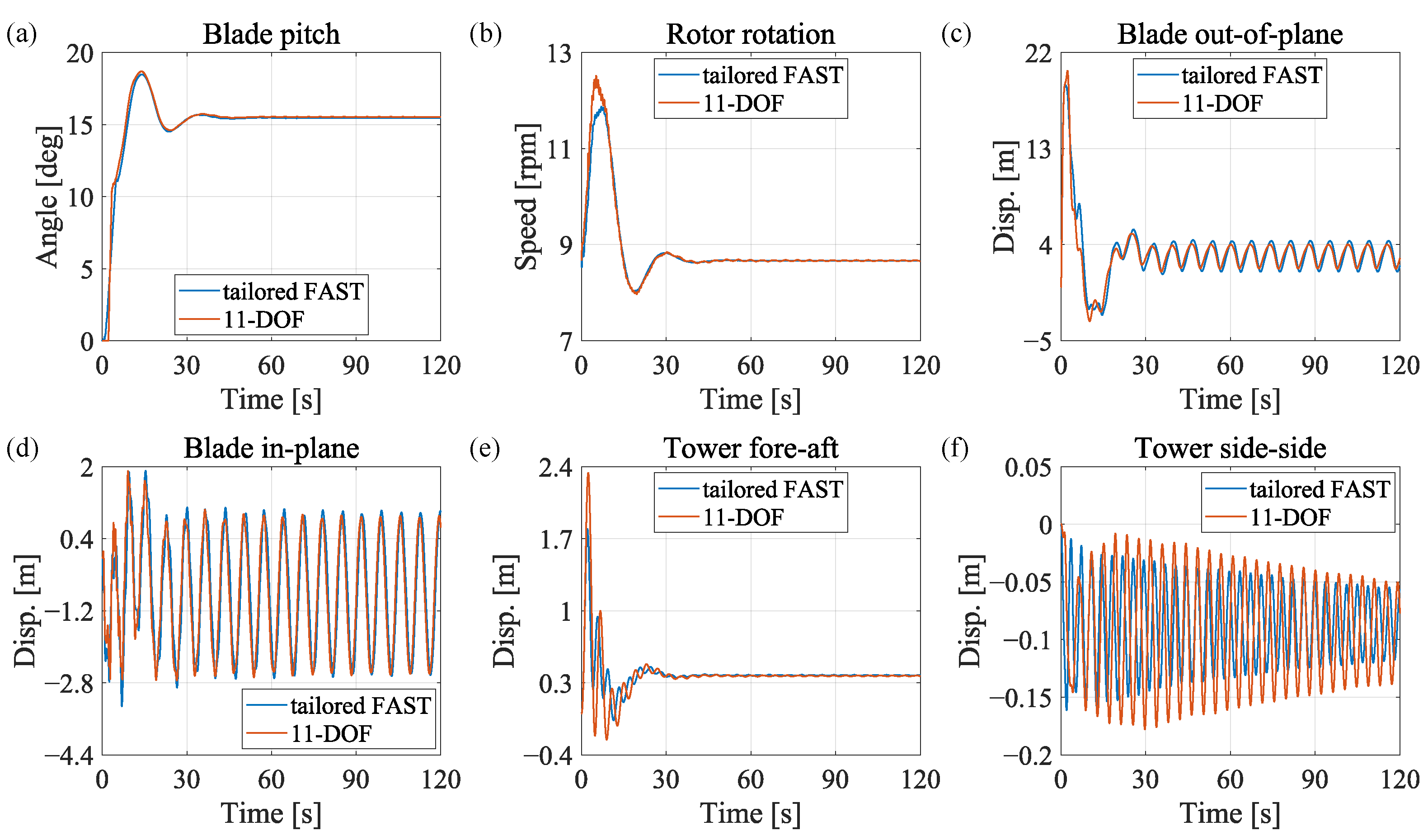
The core response results of the 10 MW OWT system, simulated by the 11-DOF fully coupled model and the tailored OpenFAST model, are given in Figure 4. Figure 4a,b present the time histories of the operational-point parameters—namely, the collective blade pitch angle and rotor speed—over 0 to 120 s. After an initial transient phase, both models exhibit high consistency in the steady-state values of these parameters. However, unlike the pitch angle, which maintains excellent agreement throughout the entire simulation, the rotor speed predicted by the 11-DOF model shows an overshoot near the peak of the transient phase. This primarily stems from minor implementation differences in the control algorithms compared with the tailored OpenFAST model, though it does not compromise the physical validity of their respective aero–servo–elastic modeling. Furthermore, Figure 4c,d show the out-of-plane and in-plane tip displacement responses of blade 1, which are transformed from the directly solved blade flapwise and edgewise DOFs, $q_1\left(t\right)$ and $q_3\left(t\right)$, based on the pitch angle. Under the influence of gravitational loads and wind shear, both the out-of-plane and in-plane steady-state responses exhibit a pronounced 1P frequency (the rotor rotational frequency). The predictions of the 11-DOF model agree closely with those of the OpenFAST model for the in-plane response, but slightly underestimates the amplitude of the steady-state response in the out-of-plane direction. This minor discrepancy is considered acceptable, as it likely arises from differences in modeling details, such as the omission of higher-order structural coupling terms in the 11-DOF model. Finally, Figure 4e,f present the tower-top, fore–aft, and side–side displacements. While the fore–aft responses are highly consistent, the side–side predictions show a more noticeable transient divergence, with the 11-DOF model yielding higher amplitudes. This behavior is primarily associated with the substantially lower aerodynamic damping of the side–side mode compared with the fore–aft mode. Based on the analytical aerodynamic damping formulation developed in [45], the first side–side modal aerodynamic damping ratio of the operational IEA 10 MW OWT is estimated to be approximately 0.2%, which is significantly lower than that of the first fore–aft mode (∼8.0%). Consequently, transient initialization differences decay more slowly in the lightly damped side–side direction before the responses converge toward steady state. In summary, the 11-DOF model demonstrates high consistency with the tailored OpenFAST model in the predictions of global trends and steady-state mean responses. Furthermore, since minor deviations in transient responses and steady-state amplitudes are ubiquitous across the simulation results from different aeroelastic codes, the proposed model is proven highly capable of analyzing the fundamental dynamic behaviors of the OWT system.

4. Dynamic Analysis of OWTs Using a Hybrid Superelement–FE Framework

This section formulates the hydroelastic tower–monopile substructure using 1D FE theory and integrates it with the proposed aero–servo–elastic superelement, establishing a hybrid modeling framework to evaluate the dynamics of the OWT system under normal and harsh environments. Consistent with the verification configuration adopted in Section 3, the support structure retains the idealized clamped-base boundary condition. This simplified configuration enables a clear demonstration of the framework’s capability in recovering high-resolution internal forces and distributed stress responses through the FE formulation. Section 4.1 outlines the synthesis of the hybrid system model and evaluates the structural modal properties of the IEA 10 MW monopile-supported OWT. Building upon this, Section 4.2 examines the displacement, force, and stress responses of the OWT operating under typical combined wind–wave loadings, while Section 4.3 investigates these structural responses under an extreme idling scenario.

4.1. Hybrid Model of the OWT System

The tower–monopile substructure, hereafter referred to as the tower for convenience, is discretized using two-node Timoshenko beam elements in a global CS consistent with that of the superelement shown in Figure 1, with each node possessing six DOFs. This is fully compatible with the six nacelle DOFs of the aero–servo–elastic superelement, enabling direct coupling of the substructures through elemental assembly. With 100 beam elements distributed along the tower height, the fully coupled OWT system yields global matrices of dimension 608 × 608, where the first six DOFs are constrained to enforce the clamped boundary condition at the base. A mesh convergence study confirmed that the adopted 100-element discretization provides converged modal characteristics, with the successive relative differences of the first 10 natural frequencies reduced to approximately 0.1% or lower. The adopted mesh therefore ensures sufficient structural accuracy for the 1D FE model while maintaining favorable computational efficiency. In addition, the structural damping matrix of the tower is constructed using the Rayleigh damping formulation, with the coefficients determined from the first two well-separated modal frequencies to account for modal-frequency-dependent damping behavior.

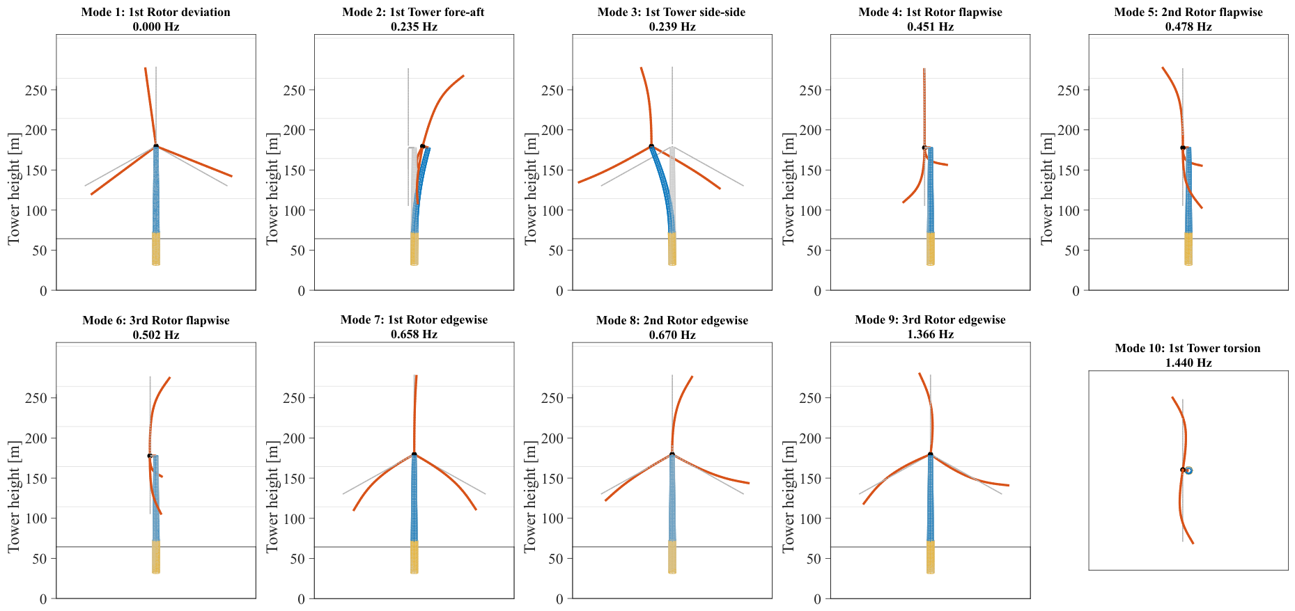
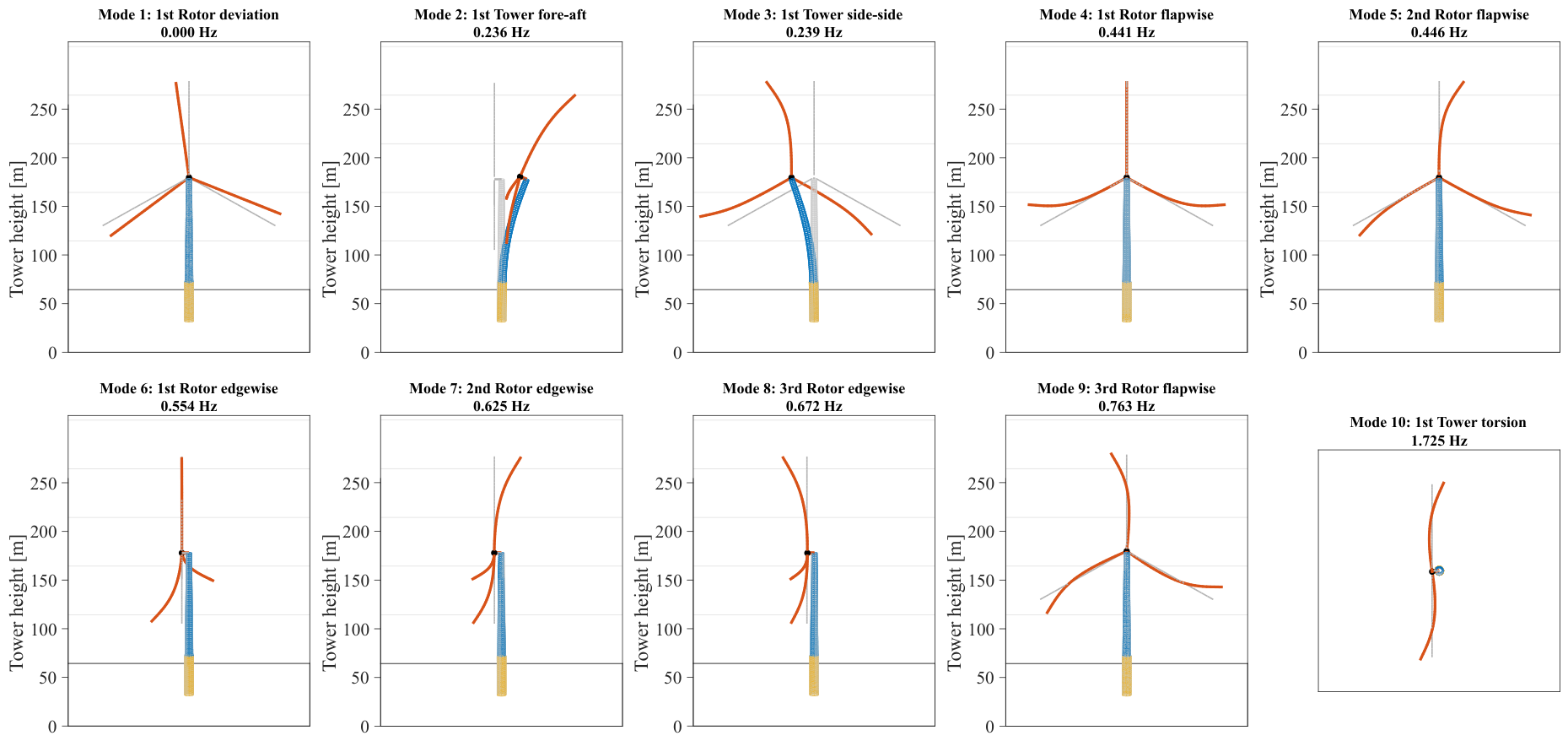
For the dynamic analysis, the structural properties are quantified using the IEA 10 MW monopile-supported OWT reference data presented in Section 3.3. An undamped structural modal analysis is then performed under an operational scenario corresponding to a mean wind speed of 15 m/s, with a rotor azimuth of $0°$, a rated rotational speed of 8.7 rpm (see Table 1), and a pith angle of $12.7°$. Figure 5 presents the first 10 mode shapes and their respective frequencies. The visualization perspectives are selected to highlight the structural deformation corresponding to the dominant modal kinetic energy. The first structural mode (Mode 1) represents rotor deviation, i.e., a near rigid-body rotational mode with negligible periodicity. Modes 2 and 3 correspond to the tower’s first fore–aft and side–side bending modes, with frequencies of approximately 0.24 Hz; in each case, more than 98% of the modal energy is concentrated in the corresponding deformation direction. Modes 4 to 6 capture the rotor flapwise dynamics (0.45–0.50 Hz), primarily associated with the fundamental vibrations of the three individual blades. Owing to the higher blade edgewise stiffness, Modes 7 to 9 correspond to the rotor edgewise dynamics at higher frequencies. While the first two edgewise modes are closely spaced (0.66 Hz and 0.67 Hz), the third increases significantly to 1.37 Hz, approaching the tower’s first torsional mode, which appears as the tenth structural mode. Due to the coupled nature of the OWT dynamics, modes dominated by a specific structural component and direction may still exhibit noticeable responses in other components and directions. For instance, Mode 4, identified as the rotor first flapwise mode, has a dominant modal kinetic energy contribution of approximately 84%, while the remaining energy is primarily associated with tower torsion, indicating a pronounced structural coupling between these motions. Similarly, in the higher-frequency Mode 10, primarily governed by tower torsion, about 15% of the modal kinetic energy is contributed by rotor flapwise motion.

Following the same convention, Figure 6 presents the first 10 modal frequencies and mode shapes of the OWT idling at a mean wind speed of 50 m/s, characterized by a rotor azimuth of $0°$, a low rotational speed of about 0.19 rpm, and a pitch angle of $90°$. Due to significant changes in rotor speed and pitch angle, both the structural mode shapes and natural frequencies are noticeably altered. The rotor flapwise modes become predominantly in-plane (within the rotor plane), whereas the edgewise modes primarily exhibit out-of-plane motion. Compared with the relatively minor variations observed in the low-frequency modes, the third flapwise mode exhibits a pronounced frequency shift, increasing from 0.50 Hz under the operating scenario to 0.76 Hz in the idling scenario. This frequency surpasses those of the first to third edgewise modes, which decrease overall, thereby becoming the ninth structural mode. In terms of motion coupling, the modal kinetic energy distribution indicates that Mode 6 and Mode 10 are respectively dominated by rotor first edgewise vibration (68.7% of the total energy) and tower torsion (66.7%). Both modes exhibit pronounced structural coupling between the blade along-wind edgewise and tower torsional vibrations.

4.2. Normal Operational Scenario

The typical scenario adopted for the OWT system features a mean wind speed of 15 m/s, a wind shear exponent and turbulence intensity both set to 0.14, and a significant wave height of 4.0 m. The wave loads are applied in the side–side direction to account for a rare wind–wave misalignment condition. Under this operational scenario, the rotor speed and power output dynamically track their rated values (as listed in Table 1) via constant generator torque and PI pitch control strategies (as described in Section 2.3).

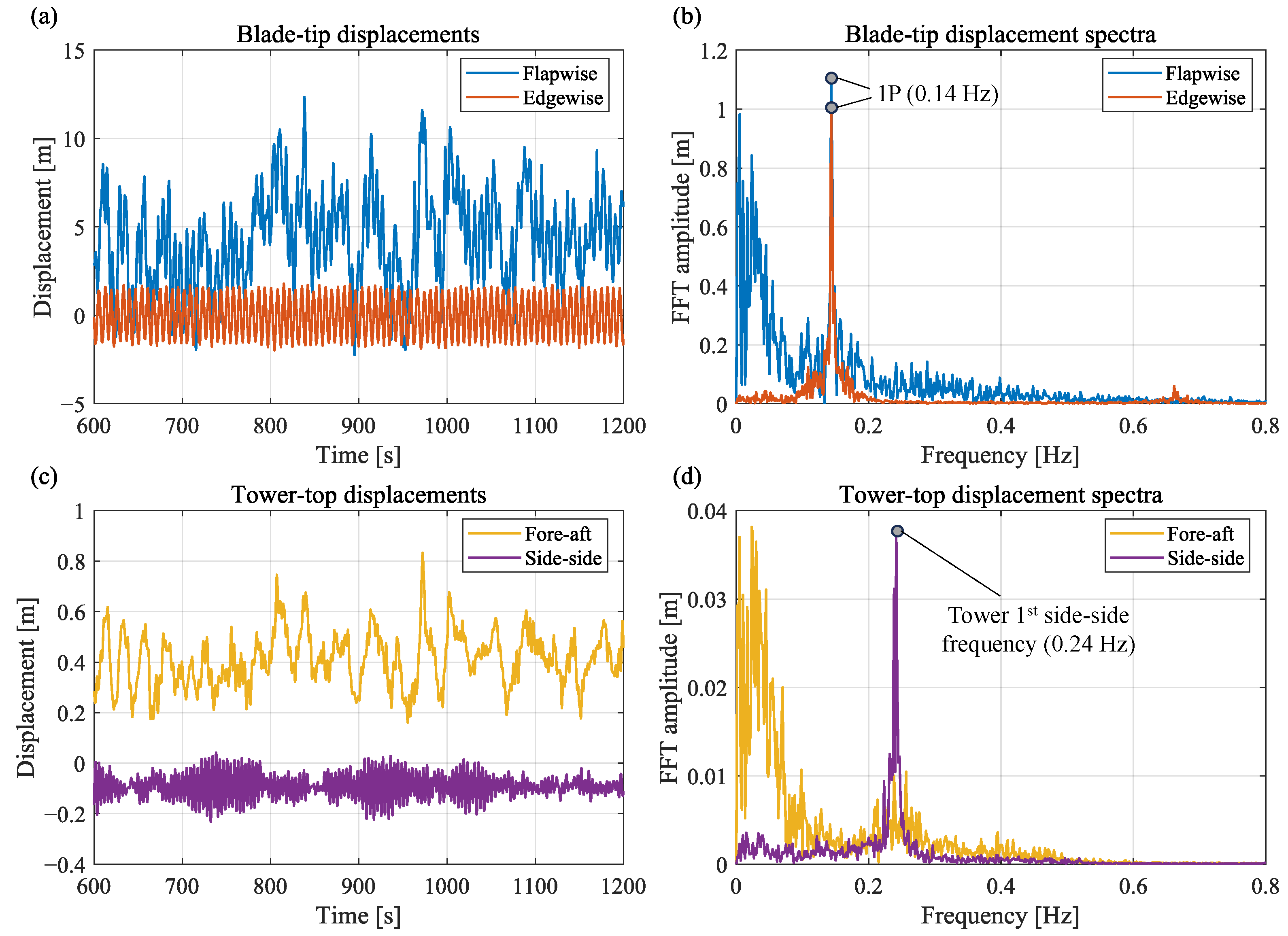
Figure 7 presents the time-domain displacement responses at the blade tip and tower top together with their corresponding frequency spectra. The spectra are included to identify dominant excitation frequencies and structural resonance characteristics that are less apparent in the time-domain responses, thereby assisting in the interpretation of the system’s dynamic behavior. Figure 7a shows the blade-tip displacements in the flapwise and edgewise directions. The irregular variation in flapwise motion—largely aligned with the incoming wind velocity—is attributed to wind shear, turbulence, gravitational loads, and the resulting pitch adjustments. This variation is, however, quasi-static due to the high aerodynamic damping of the flapwise mode [45]. In contrast, the edgewise displacement, which lies approximately within the rotor plane, is dominated by gravitational loads, exhibiting a near-zero mean and pronounced harmonic-like characteristics. As illustrated in Figure 7b, compared with the edgewise response, which is almost exclusively concentrated at the 1P excitation frequency due to rotationally asymmetric effects, the flapwise response additionally exhibits high amplitudes in the low-frequency region driven by turbulence. Furthermore, Figure 7c,d display the time- and frequency-domain displacement responses of the tower top in the fore–aft and side–side directions. Similar to the flapwise dynamics, the fore–aft vibration of the tower, aligned with the along-wind direction, concentrates in the low-frequency region. Notably, the tower’s first side–side mode with a natural frequency of 0.24 Hz is significantly excited by the combined wind–wave loading, resulting in significant resonant behavior in the side–side displacement shown in Figure 7c. The observed strong dynamic amplification effect is fundamentally tied to the inherently low aerodynamic damping of the tower side–side mode [45].

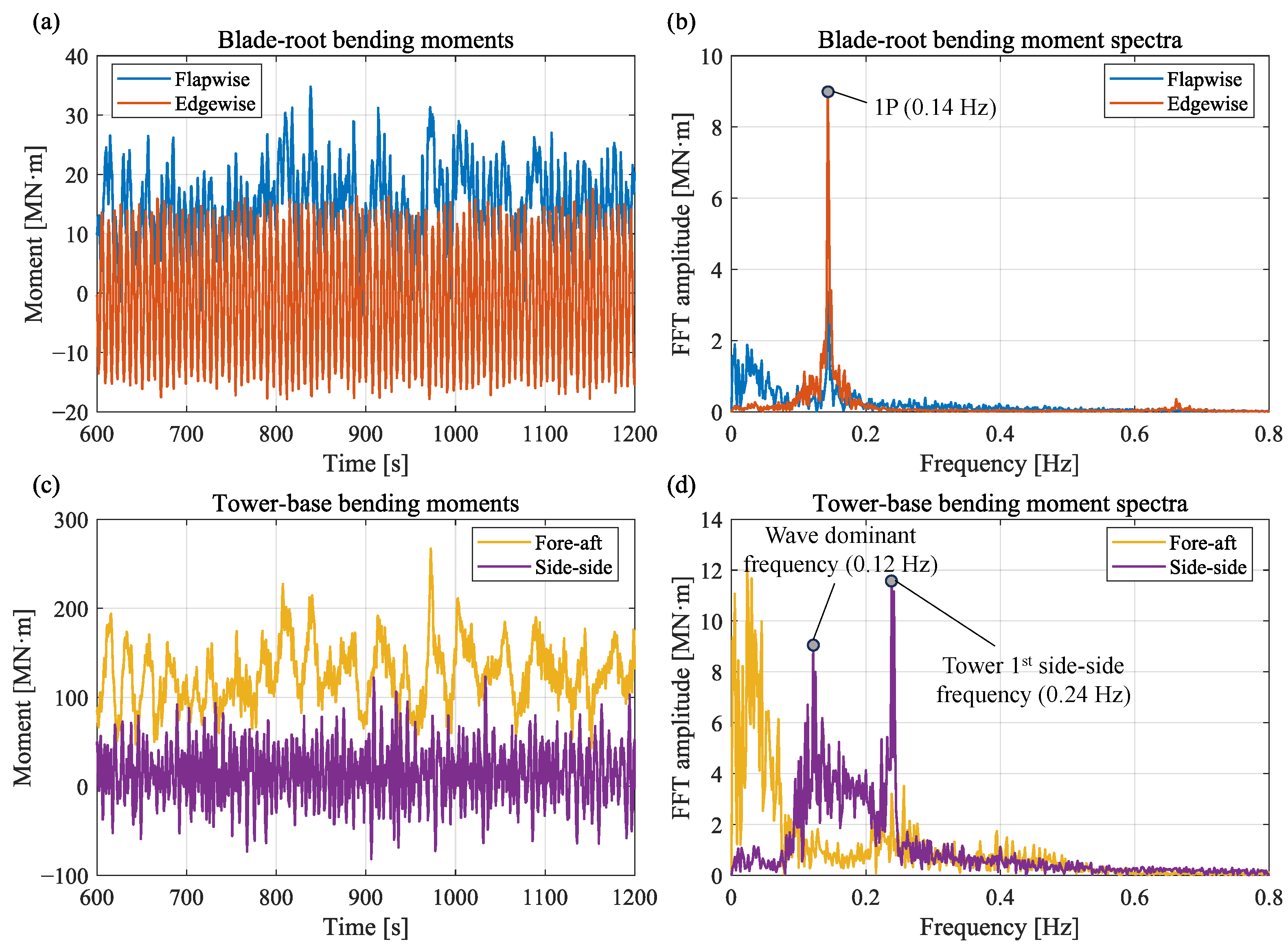
Figure 8 presents the bending moments at the blade root and tower base of the OWT. As anticipated, the blade-root bending moments in Figure 8a,b closely mirror the blade-tip displacement characteristics in Figure 7a,b, particularly regarding the pronounced 1P–dominated frequency and the amplitude peaks in the low-frequency region for the quasi-static flapwise response. However, in stark contrast to the relatively low spectral peak of the edgewise displacement in Figure 7a, the amplitude of the edgewise bending moment in Figure 8a significantly surpasses its flapwise counterpart. This amplification is driven by the higher edgewise structural stiffness, indicating a critical concern for fatigue damage. It is worth noting that the bending moments at the blade root cannot be calculated using the mode shape polynomials inherent to the modal-based formulation of the superelement. The primary reason is that the curvature at the highly stiff blade root is extremely small in magnitude (on the order of ${10}^{-4}$ for this case). In this context, using sixth-order polynomial fits of the blade mode shapes (${\Phi }_f$ and ${\Phi }_e$) to evaluate such minute curvatures can introduce substantial relative errors. Instead, the blade-root bending moments are reconstructed through direct superposition of the aerodynamic, gravitational, and inertial load components, which are associated with the underlying velocity- and acceleration-dependent dynamics. This highlights the inherent advantage of the FE theory over the modal approach in computing internal forces, as it can directly calculate accurate curvatures at prescribed cross-sections through post-processing of the densely discretized DOF field. Figure 8c,d present the tower-base fore–aft and side–side bending moments, which are directly obtained by multiplying these FE-derived curvatures by the corresponding sectional stiffnesses. The time- and frequency-domain characteristics of the fore–aft bending moment at the tower base closely align with those of the tower-top fore–aft displacements shown in Figure 7c,d. However, compared with the tower-top side–side displacement, the tower-base side–side bending moment not only features a resonance peak corresponding to the first side–side frequency of the tower, but also exhibits a distinct spectral peak matching the peak wave period, as shown in Figure 8d.

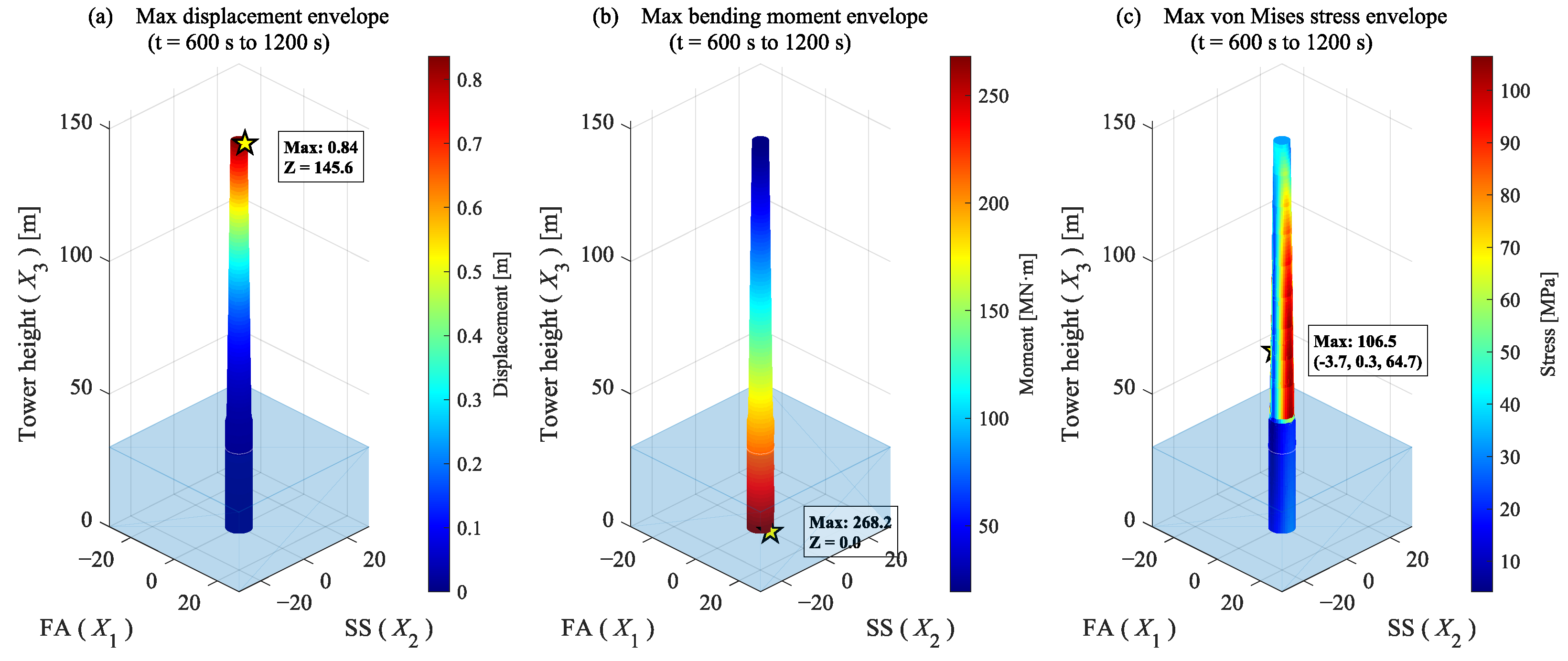
Based on the displacement response field from the 1D FE model of the tower, Figure 9a,b present the envelopes of maximum displacement and maximum bending moment over time along the tower height. Here, the displacement refers to the horizontal resultant magnitude synthesized from the fore–aft and side–side components, with axial deformation neglected due to its relatively small contribution. As shown in Figure 9a, the maximum tower displacement occurs at the tower top ($X_3$ = 145.6 m) with a value of 0.84 m. This displacement decreases monotonically with decreasing height, reaching zero at the clamped tower base. Conversely, the maximum bending moment in Figure 9b increases continuously toward the base, attaining a peak value of 268.2 MN·m. Furthermore, Figure 9c presents the spatial envelope of the maximum von Mises stress over the entire tower based on equivalent beam theory. Unlike the monotonic trends observed in the displacement and bending moment envelopes, the stress level in the monopile section is markedly lower than that in the tower section, primarily due to the abrupt increase in sectional stiffness at the tower–monopile transition. In addition, since the sectional stiffness of the tower—governed by its inner and outer diameters—decreases toward the tower top, a high-stress region extends over a considerable length, as indicated by the red area in Figure 9c. Consequently, under this combined wind–wave loading condition, the global maximum von Mises stress over both time and space occurs at $X_3=64.7$ m, rather than at the bottom of the tower section ($X_3=40$ m). From an engineering perspective, the maximum stress of 106.5 MPa remains well below the yield strength of typical wind turbine tower steels (e.g., S355 steel). In addition, the recovered spatial stress distributions provide useful insight into the localization of high-stress regions, which is relevant for structural optimization and material-efficient tower design.

4.3. Extreme Idling Scenario

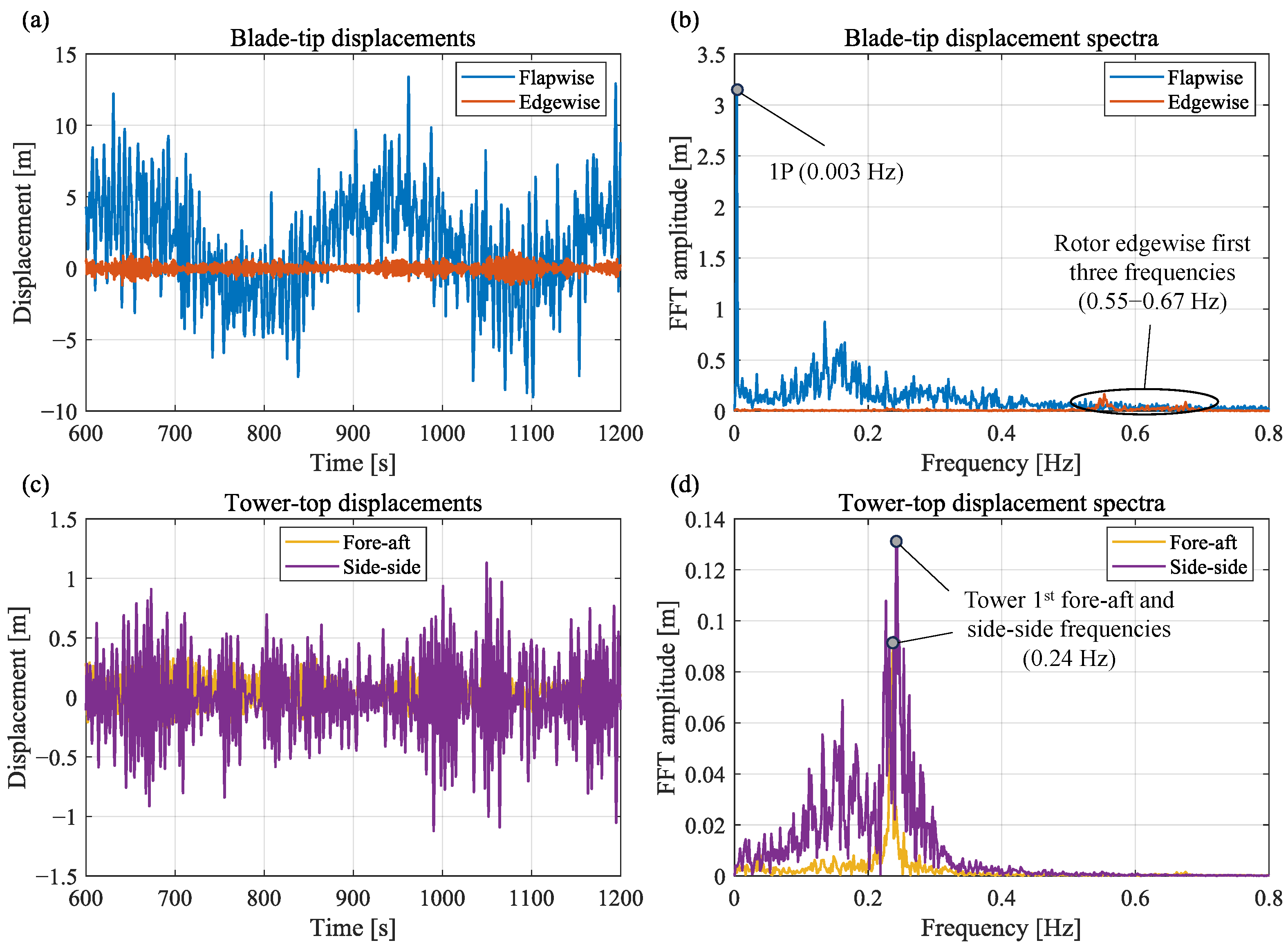
The extreme idling scenario evaluated for the OWT system features a 50-year return period wind speed of 50 m/s, a wind shear exponent and turbulence intensity both set to 0.11, and a significant wave height of 10.0 m applied in the side–side direction. In this state, the three blades are feathered to $90°$, the servo control is deactivated, and the rotor idles at a minimal speed. Figure 10a presents the corresponding displacement time histories at the blade tip and tower top. Due to blade feathering, the cross-wind flapwise response under the extreme idling scenario exhibits displacement amplitudes comparable to those under the normal operational scenario (Figure 7a). This mitigation of aerodynamic loading effects is more evident in the edgewise response, where gravitational load components are currently absent in this direction. As shown in Figure 10a, the edgewise displacement under extreme wind speed is even lower than its operational counterpart (Figure 7), despite the emergence of resonance behavior observed in Figure 10b. Additionally, turbulence continues to introduce the relatively low-frequency components in the flapwise displacement. Comparing Figure 7b and Figure 10b shows that when the OWT shifts from rated operation to low-speed idling, the 1P frequency dominating the flapwise vibration decreases from 0.14 Hz to 0.003 Hz. Conversely, the edgewise vibration becomes dominated by resonance frequencies of 0.55–0.67 Hz, rendering the 1P effect negligible. Figure 10c,d show that the tower-top fore–aft and side–side displacements both exhibit resonance behavior under combined wind–wave loading, with a dominant frequency of approximately 0.24 Hz, consistent with the structural natural frequency identified in Figure 6. Furthermore, due to blade feathering, the tower side–side direction aligns with the blade flapwise direction; consequently, the corresponding low-frequency response (Figure 10d) exhibits a distribution pattern similar to that of the flapwise response (Figure 10b), with minimal influence from wave excitation.

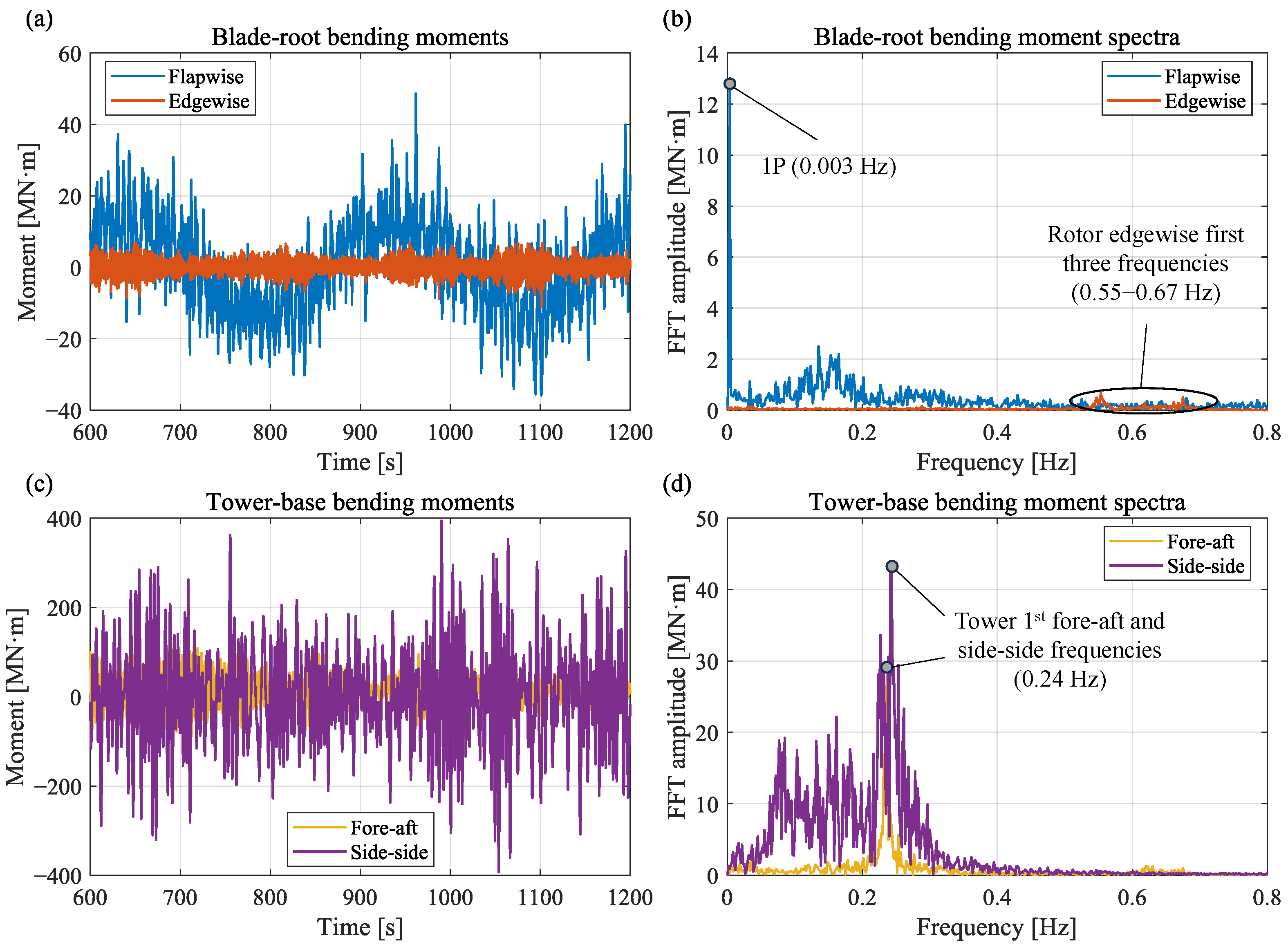
The response characteristics of the blade-root and tower-base bending moments shown in Figure 11 are highly consistent with those in Figure 10. For the blade-root moments in Figure 11a,b, the in-plane flapwise bending moment response is primarily governed by the 1P loading and low-frequency turbulent excitation, whereas the out-of-plane edgewise bending moment is dominated by its resonance frequencies. Although the steady aerodynamic loading is significantly reduced due to blade feathering, the flapwise bending moment remains at a relatively high level under the combined effects of gravity and turbulence. The tower-base, fore–aft, and side–side bending moments shown in Figure 11c,d are also consistently dominated by their corresponding resonance frequencies. However, comparison between Figure 10 and Figure 11d indicates that wave excitation contributes more noticeably to the low-frequency response of the tower-base bending moment than to the tower-top displacement, which is consistent with the characteristics of wave loading under operational scenario (Figure 7 and Figure 8d).

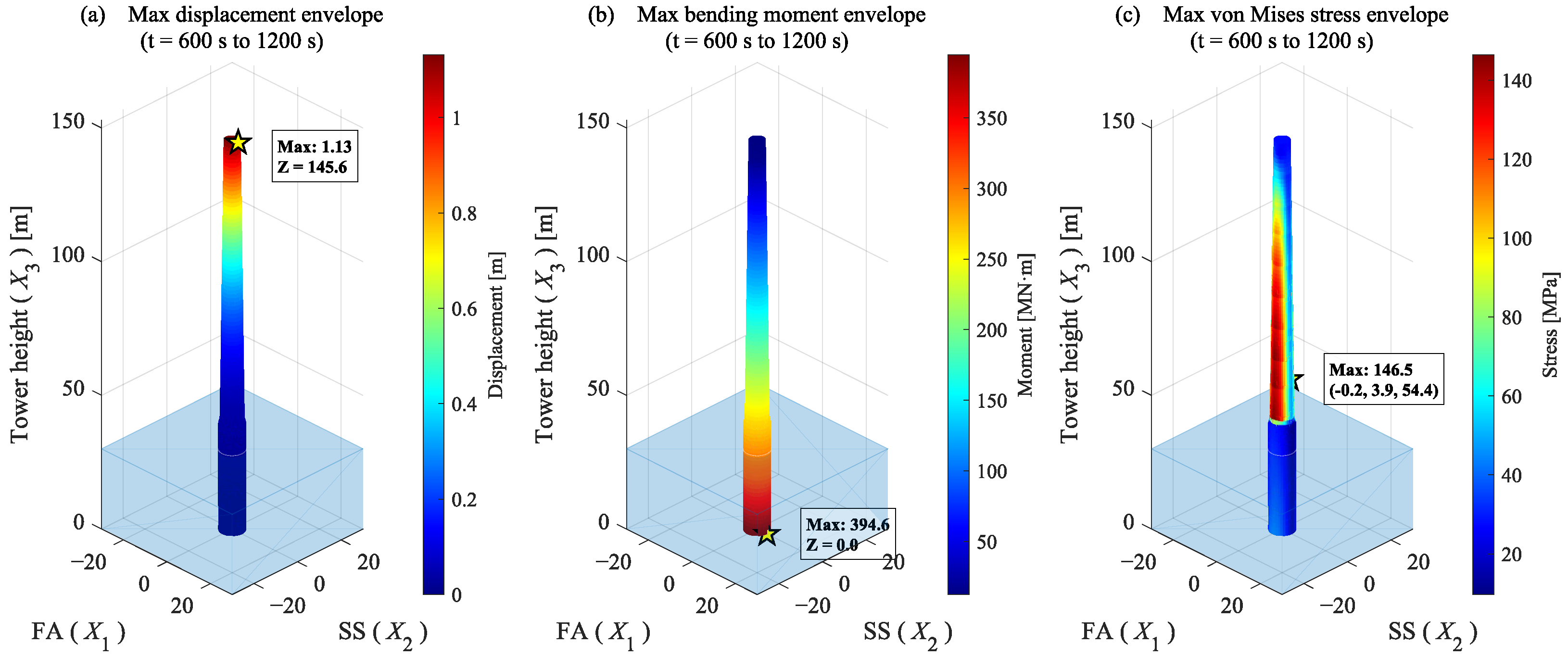
Figure 12 presents the envelope of maximum structural response of the tower under the extreme idling scenario, following the same plotting convention as in Figure 9. Similarly, as shown in Figure 12a,b, the envelopes of maximum displacement and maximum bending moment also exhibit monotonic variations with height. This behavior is essentially a manifestation of the tower vibration being dominated by its fundamental mode. Compared with the normal operating scenario, the maximum tower-top displacement increases to 1.13 m, while the maximum tower-base bending moment reaches 394.6 MN·m, corresponding to increases of 34.5% and 47%, respectively. Although these increases are significant, they are entirely acceptable as the cost of withstanding extreme wind–wave loading, providing direct evidence of the highly effective structural protection afforded by blade feathering. The maximum stress contour distribution under the extreme idling scenario (Figure 12c) is, however, different from that under the operational scenario (Figure 9c). Roughly speaking, the present stress distribution pattern in Figure 12c can be interpreted as a 90° rotation of that in Figure 9c. This is because blade feathering reverses the alignment relationship between the tower fore–aft/side–side directions and the blade flapwise/edgewise directions. Consequently, the high-stress region switches from the along-wind side to the cross-wind side. Accordingly, the global maximum stress occurs at the cross-section located at an elevation of 54.4 m, with a side–side coordinate of $X_2=3.9$ m, while the fore–aft coordinate is $X_1=-0.2$ m. The peak von Mises stress reaches 144.7 MPa, which, although significantly amplified compared with the operational scenario, still remains well below the yield strength of commonly used structural steels. More importantly, the circumferential shift of the high-stress region suggests that fatigue-critical locations may vary with the operating state of the OWT. The proposed hybrid framework enables such spatially varying stress distributions to be resolved continuously in the time domain.

4.4. Limitations of the Present Implementation

The present study establishes and verifies a hybrid aero–servo–hydro–elastic modeling framework for OWTs by coupling a reduced-order rotor–nacelle superelement with a FE-based support structure. Although dynamic analyses utilizing this framework demonstrate favorable capability in predicting global structural dynamics and recovering distributed internal force and stress responses, several modeling simplifications remain in the current demonstrative implementation.

On the rotor–nacelle side, the proposed superelement retains only the blade first flapwise and first edgewise modes and employs quasi-steady aerodynamics. Such a reduced-order representation is intended to capture the dominant low-frequency aero–servo–elastic behavior under typical scenarios while preserving physically consistent coupling with the support-structure system and accurate transmission of aerodynamic loading through the nacelle DOFs. Consequently, higher-frequency blade dynamics as well as unsteady aerodynamic effects (e.g., dynamic stall and dynamic wake) are not explicitly incorporated in the current study. These simplifications may influence the prediction accuracy for loading conditions involving rapidly varying inflow conditions or stronger higher-mode participation. On the support-structure side, the present work adopts a demonstrative monopile-supported configuration with an idealized clamped-base boundary condition and a 1D FE representation to provide a consistent verification configuration for the proposed hybrid framework. Within this implementation, foundation-related effects, including soil–structure interaction and alternative support-structure configurations (e.g., jacket-type and floating foundations), are not considered. In addition, although the adopted 1D FE formulation is effective for global structural response analysis and recovery of distributed internal force and stress responses, detailed three-dimensional local structural behavior cannot be fully resolved.

Nevertheless, these assumptions are associated with the current demonstrative implementation rather than the hybrid coupling framework itself. Owing to the general interface-based formulation adopted in the present study, the framework can be systematically extended in future work to incorporate higher-order blade representations, more advanced aerodynamic and hydrodynamic load models, and higher-fidelity support-structure formulations, including soil-interacting foundations, floating systems, and 3D FE models.

5. Conclusions

In this study, an efficient hybrid modeling framework is proposed for the dynamic analysis of offshore wind turbines (OWTs) by integrating an aero–servo–elastic rotor–nacelle superelement with a hydroelastic substructure. The governing equations of the 14-DOF superelement are derived analytically using a modal-based multibody dynamics formulation, capturing the rigorous aeroelastic coupling and spinning effects governed by structural deformation, nonlinear aerodynamics, and active servo controls. By matching the interface degrees of freedom at the nacelle, this superelement can be dynamically coupled with either a finite element (FE) model of the substructure or a physical laboratory substructure. This versatility establishes a robust foundation for high-fidelity system hybrid formulation, co-simulations, and real-time hybrid simulations. To validate the analytical formulation of the superelement, an 11-DOF fully coupled OWT model was first verified against a tailored OpenFAST model using a similar modal-based formulation, demonstrating high consistency in predicting both transient and steady-state dynamics. Building upon this validated superelement, the proposed hybrid architecture—integrating the superelement with a 1D FE substructure model as an example—resolves the challenge of internal force recovery. It guarantees high computational efficiency and rigorous aerodynamic coupling and damping effects via the 14-DOF analytically derived superelement, while utilizing the high-resolution FE tower–monopile model to accurately compute local curvatures and strains for superior internal force and stress evaluations. Leveraging these capabilities, the demonstrative dynamic analyses of the IEA 10 MW OWT yielded the following key insights:

• Under the typical operational scenario, the blade-tip flapwise/edgewise displacements and their corresponding root bending moments exhibit pronounced 1P characteristics due to non-axisymmetric loads. The edgewise response, less susceptible to turbulence, demonstrates clear quasi-harmonic behavior. The tower fore–aft responses mirror the near-aligned flapwise dynamics in the low-frequency region, whereas the side–side responses experience significant resonance.
• Under the extreme idling scenario, blade flapwise responses remain 1P-dominated, while edgewise motions exhibit resonance. Blade feathering aligns the tower side–side motion with the blade flapwise vibration, yielding similar spectral distributions in the low-frequency region between them. Moreover, both tower fore–aft and side–side responses develop pronounced resonance peaks.
• Unlike the monotonic displacement and moment envelopes, the maximum stress envelope distributes non-monotonically, with its high-stress region concentrating broadly in mid-lower tower sections characterized by lower stiffness and larger bending moments. The blade feathering mechanism shifts this high-stress region from the along-wind to the cross-wind side due to the altered kinematic correspondence.

Future work will focus on extending the present hybrid framework toward higher-fidelity aero-servo-hydro-elastic simulations by incorporating higher-order structural representations, more advanced unsteady aerodynamic and hydrodynamic models, and enhanced support-structure formulations accounting for soil–structure interaction and various foundation configurations.

References

1. Global Wind Energy Council. Global Wind Report 2025; Technical report; Global Wind Energy Council (GWEC): Brussels, Belgium, 2025. [Google Scholar]
2. Xie, F.; Aly, A.M. Structural control and vibration issues in wind turbines: A review. Eng. Struct. 2020, 210, 110087. [Google Scholar] [CrossRef]
3. He, G.; Zhao, C.; Cui, T.; Luan, Z.; Liu, C.; He, R. A review of hydrodynamic response and mitigation strategies of floating offshore wind turbines under extreme conditions. Ocean Eng. 2026, 355, 125140. [Google Scholar] [CrossRef]
4. Chen, W.L.; Zhang, Z.; Liu, J.; Gao, D. Experimental study on dynamic characteristics of a jacket-type offshore wind turbine under coupling action of wind and wave. Appl. Energy 2025, 378, 124876. [Google Scholar] [CrossRef]
5. Cao, Q.; Xiao, L.; Cheng, Z.; Liu, M.; Wen, B. Operational and extreme responses of a new concept of 10MW semi-submersible wind turbine in intermediate water depth: An experimental study. Ocean Eng. 2020, 217, 108003. [Google Scholar] [CrossRef]
6. Ren, Y.; Shi, W.; Venugopal, V.; Zhang, L.; Li, X. Experimental study of tendon failure analysis for a TLP floating offshore wind turbine. Appl. Energy 2024, 358, 122633. [Google Scholar] [CrossRef]
7. Jia, X.; Liang, F.; Zhang, H.; Cui, W.; Zhong, G. A wind-current flume study of scour and remediation effects on dynamics of monopile offshore wind turbines during operation and typhoon-induced shutdown. Ocean Eng. 2026, 357, 125538. [Google Scholar] [CrossRef]
8. Sun, C.; Song, W.; Jahangiri, V. A real-time hybrid simulation framework for floating offshore wind turbines. Ocean Eng. 2022, 265, 112529. [Google Scholar] [CrossRef]
9. Huang, H.; Liu, Q.; Iglesias, G.; Li, C. Advanced multi-physics modeling of floating offshore wind turbines for aerodynamic design and load management. Energy Convers. Manag. 2025, 346, 120437. [Google Scholar] [CrossRef]
10. Miao, W.; Li, C.; Wang, Y.; Xiang, B.; Liu, Q.; Deng, Y. Study of adaptive blades in extreme environment using fluid–structure interaction method. J. Fluids Struct. 2019, 91, 102734. [Google Scholar] [CrossRef]
11. Shyam, A.; Aryan, A.S.; Shailesh, C.; Harigovind, R.; Vipin, V.; Krishnan, A. Design and analysis of small-scale horizontal axis wind turbine using PVC material. Mater. Today Proc. 2022, 52, 2238–2254. [Google Scholar] [CrossRef]
12. Liu, Y.; Li, N.; Wang, P.; Wang, T.; Zhou, J.; Qin, Z.; Chu, F. A review of vibration analysis and suppression for wind turbine blades: State of the art, challenges and perspectives. Thin-Walled Struct. 2026, 218, 114095. [Google Scholar] [CrossRef]
13. Jiang, S.; Duan, S. A Multibody Dynamics Approach for Vibration Analysis of Horizontal Axis Wind Turbine Blades. In Proceedings of the ASME 2016 International Mechanical Engineering Congress and Exposition; American Society of Mechanical Engineers: New York, NY, USA, 2016; Volume 4. [Google Scholar] [CrossRef]
14. Mo, W.; Li, D.; Wang, X.; Zhong, C. Aeroelastic coupling analysis of the flexible blade of a wind turbine. Energy 2015, 89, 1001–1009. [Google Scholar] [CrossRef]
15. Xu, J.; Zhang, L.; Li, X.; Li, S.; Yang, K. A study of dynamic response of a wind turbine blade based on the multi-body dynamics method. Renew. Energy 2020, 155, 358–368. [Google Scholar] [CrossRef]
16. Zhao, X.; Maißer, P.; Wu, J. A new multibody modelling methodology for wind turbine structures using a cardanic joint beam element. Renew. Energy 2007, 32, 532–546. [Google Scholar] [CrossRef]
17. Hansen, M.; Sørensen, J.; Voutsinas, S.; Sørensen, N.; Madsen, H. State of the art in wind turbine aerodynamics and aeroelasticity. Prog. Aerosp. Sci. 2006, 42, 285–330. [Google Scholar] [CrossRef]
18. Timoshenko, S. History of Strength of Materials; McGraw-Hill: Columbus, OH, USA, 1953. [Google Scholar]
19. Hodges, D.H. Geometrically Exact, Intrinsic Theory for Dynamics of Curved and Twisted Anisotropic Beams. AIAA J. 2003, 41, 1131–1137. [Google Scholar] [CrossRef]
20. Wu, H.; Ke, S.; Ren, H.; Tian, W.; Wang, H.; Zhu, S.; Wang, T. An efficient reduced-order modeling framework for spatiotemporal aerodynamic damping in flexible wind turbine blades. Phys. Fluids 2025, 37, 055149. [Google Scholar] [CrossRef]
21. Zienkiewicz, O.C.; Taylor, R.L. The Finite Element Method for Solid and Structural Mechanics; Elsevier: Amsterdam, The Netherlands, 2005. [Google Scholar]
22. Hilber, H.M.; Hughes, T.J.R.; Taylor, R.L. Improved numerical dissipation for time integration algorithms in structural dynamics. Earthq. Eng. Struct. Dyn. 1977, 5, 283–292. [Google Scholar] [CrossRef]
23. Hodges, D.H.; Pierce, G.A. Introduction to Structural Dynamics and Aeroelasticity, 2nd ed.; Cambridge Aerospace Series; Cambridge University Press: Cambridge, UK, 2011. [Google Scholar] [CrossRef]
24. Li, X.; Xu, Z.; Basu, B.; Alujevic, N.; Habib, G.; Zhang, Z. Dynamic modeling and analysis of gyroscopic effects in bottom-fixed wind turbines under normal and extreme wind conditions. Renew. Energy 2026, 256, 124678. [Google Scholar] [CrossRef]
25. Zhang, Z.; Li, X.; Larsen, T.G.; Sun, T.; Yang, Q. Pole-Placement-Based Calibration of an Electromagnetically Realizable Inerter-Based Vibration Absorber (IDVA) for Rotating Wind Turbine Blades. Struct. Control Health Monit. 2024, 2024, 7255774. [Google Scholar] [CrossRef]
26. Insam, C.; Rixen, D.J. Fidelity assessment of Real-Time Hybrid Substructuring based on convergence and extrapolation. Mech. Syst. Signal Process. 2022, 175, 109135. [Google Scholar] [CrossRef]
27. Zhang, Z.; Staino, A.; Basu, B.; Nielsen, S.R. Performance evaluation of full-scale tuned liquid dampers (TLDs) for vibration control of large wind turbines using real-time hybrid testing. Eng. Struct. 2016, 126, 417–431. [Google Scholar] [CrossRef]
28. Zhang, Z.; Basu, B.; Nielsen, S.R. Real-time hybrid aeroelastic simulation of wind turbines with various types of full-scale tuned liquid dampers. Wind Energy 2019, 22, 239–256. [Google Scholar] [CrossRef]
29. Song, W.; Sun, C.; Zuo, Y.; Jahangiri, V.; Lu, Y.; Han, Q. Conceptual Study of a Real-Time Hybrid Simulation Framework for Monopile Offshore Wind Turbines Under Wind and Wave Loads. Front. Built Environ. 2020, 6, 129. [Google Scholar] [CrossRef]
30. Ha, Y.J.; Ahn, H.; Park, S.; Park, J.Y.; Kim, K.H. Development of hybrid model test technique for performance evaluation of a 10 MW class floating offshore wind turbine considering asymmetrical thrust. Ocean Eng. 2023, 272, 113783. [Google Scholar] [CrossRef]
31. National Renewable Energy Laboratory (NREL). OpenFAST Documentation; National Renewable Energy Laboratory: Golden, CO, USA, 2026.
32. Xu, J.; He, Z.; Wang, D.; He, G.; Wu, Q.; Zhang, Z. Nonlinear dynamic response analyses of Onshore Wind Turbines with Steel–Concrete Hybrid Tower using a co-simulation approach. Renew. Energy 2025, 243, 122475. [Google Scholar] [CrossRef]
33. Wang, D.; Xu, J.; He, Z.; Yu, Q.; Tang, W.; He, G.; Wu, Q. High-fidelity integrated co-simulation model for dynamic analysis of onshore wind turbines with Steel–Concrete Hybrid Tower. Mech. Syst. Signal Process. 2025, 230, 112583. [Google Scholar] [CrossRef]
34. Zhang, Z. Passive and Active Vibration Control of Renewable Energy Structures. Ph.D. Thesis, Aalborg University, Aalborg, Denmark, 2015. [Google Scholar] [CrossRef]
35. Humar, J. Dynamics of Structures; CRC Press: Boca Raton, FL, USA, 2012. [Google Scholar]
36. Shabana, A.A. Dynamics of Multibody Systems; Cambridge University Press: Cambridge, UK, 2020. [Google Scholar]
37. Hansen, M. Aerodynamics of Wind Turbines; Routledge: London, UK, 2015. [Google Scholar] [CrossRef]
38. Smith, S.W. The Scientist and Engineer’s Guide to Digital Signal Processing; California Technical Publishing: San Diego, CA, USA, 1997. [Google Scholar]
39. Ogata, K.; Yang, Y. Modern Control Engineering; Prentice Hall: New York, NY, USA, 2002; Volume 5. [Google Scholar]
40. Jonkman, J.; Butterfield, S.; Musial, W.; Scott, G. Definition of a 5MW Reference Wind Turbine for Offshore System Development; Technical report; National Renewable Energy Laboratory (NREL): Golden, CO, USA, 2009. [CrossRef]
41. Bortolotti, P.; Tarres, H.C.; Dykes, K.L.; Merz, K.; Sethuraman, L.; Verelst, D.; Zahle, F. IEA Wind TCP Task 37: Systems Engineering in Wind Energy—WP2.1 Reference Wind Turbines; Technical report; National Renewable Energy Laboratory (NREL): Golden, CO, USA, 2019. [CrossRef]
42. Abbas, N.; Zalkind, D.; Pao, L.; Wright, A. A Reference Open-Source Controller for Fixed and Floating Offshore Wind Turbines. Wind Energy Sci. Discuss. 2021, 2021, 1–33. [Google Scholar] [CrossRef]
43. Faltinsen, O. Sea Loads on Ships and Offshore Structures; Cambridge University Press: Cambridge, UK, 1990. [Google Scholar]
44. Robertson, A.N.; Wendt, F.; Jonkman, J.M.; Popko, W.; Borg, M.; Bredmose, H.; Schlutter, F.; Qvist, J.; Bergua, R.; Harries, R.; et al. OC5 project phase Ib: Validation of hydrodynamic loading on a fixed, flexible cylinder for offshore wind applications. Energy Procedia 2016, 94, 82–101. [Google Scholar] [CrossRef]
45. Li, X.; Basu, B.; Habib, G.; Zhang, Z. Closed-form solution to multi-mode aerodynamic damping of monopile-supported offshore wind turbines. Eng. Struct. 2025, 332, 119993. [Google Scholar] [CrossRef]
Figure 1. The OWT model described by the DOFs q 1 ( t ) , q 2 ( t ) , , q 13 ( t ) and q 14 ( t ) , along with the global and local coordinate systems.
Jmse 14 01001 g001
Figure 2. The airfoil at x 3 -position on blade j subjected to the nonlinear aerodynamic loads (the dependency on x 3 is omitted in the notations for conciseness).
Jmse 14 01001 g002
Figure 3. Schematic of a modal-based OWT model coupling the aero–servo–elastic rotor–nacelle superelement and a 3-DOF ( q t 1 , q t 2 , q t 3 ) hydrodynamic tower–monopile substructure.
Jmse 14 01001 g003
Figure 4. Dynamic responses of the 11-DOF model and the tailored OpenFAST model under a hub-height mean wind speed of 17 m/s and wind shear exponent of 0.1. ( a ) Collective pitch angle, ( b ) rotor rotational speed, ( c ) blade-tip out-of-plane displacement, ( d ) blade-tip in-plane displacement, ( e ) tower-top fore–aft displacement, ( f ) tower-top side–side displacement.
Jmse 14 01001 g004
Figure 5. Modal frequencies and mode shapes of the hybrid OWT system model derived at a normal operational scenario, characterized by a zero rotor azimuth and a mean wind speed of 15 m/s (red lines: blades; blue region: tower; yellow region: monopile).
Jmse 14 01001 g005
Figure 6. Modal frequencies and mode shapes of the hybrid OWT system model derived at an extreme idling scenario, characterized by a zero rotor azimuth and a mean wind speed of 50 m/s (red lines: blades; blue region: tower; yellow region: monopile).
Jmse 14 01001 g006
Figure 7. Structural displacements of the operating OWT system under the combined wind–wave loading (mean wind speed 15 m/s, wind shear exponent 0.14, turbulence intensity 0.14, significant wave height 4.0 m). (a) time- and (b) frequency-domain blade-tip displacements in the flapwise and edgewise directions, (c) time- and (d) frequency-domain tower-top displacements in the fore–aft and side–side directions. (Note in (b) that the blade flapwise and edgewise vibrations are dominated by the 1P frequency of 0.14 Hz).
Jmse 14 01001 g007
Figure 8. Structural bending moments of the operating OWT system under the combined wind–wave loading. (a) time- and (b) frequency-domain blade-root bending moments associated with flapwise and edgewise motions, (c) time- and (d) frequency-domain tower-base bending moments associated with fore–aft and side–side motions.
Jmse 14 01001 g008
Figure 9. Maximum tower response envelopes of the operating OWT system under the combined wind–wave loading. (a) Maximum displacement envelope, (b) maximum bending moment envelope; (c) maximum von Mises stress envelope. Note that the responses in (a,b) are distributed along the tower height, whereas the stress in (c) is distributed along both the height and circumference.
Jmse 14 01001 g009
Figure 10. Structural displacements of the idling OWT system under the combined wind–wave loading (mean wind speed 50 m/s, wind shear exponent 0.11, turbulence intensity 0.11, significant wave height 10.0 m). (a) time- and (b) frequency-domain blade-tip displacements in the flapwise and edgewise directions, (c) time- and (d) frequency-domain tower-top displacements in the fore–aft and side–side directions. (Note that the 1P frequency shown here in (b) decreases to 0.003 Hz, and the edgewise vibration shifts to being dominated by resonance frequencies of 0.55–0.67 Hz (compared with Figure 7b).
Jmse 14 01001 g010
Figure 11. Structural bending moments of the idling OWT system under the combined wind–wave loading. (a) time- and (b) frequency-domain blade-root bending moments associated with flapwise and edgewise motions, (c) time- and (d) frequency-domain tower-base bending moments associated with fore–aft and side–side motions.
Jmse 14 01001 g011
Figure 12. Maximum tower response envelopes of the idling OWT system under the combined wind–wave loading. (a) Maximum displacement envelope, (b) maximum bending moment envelope; (c) maximum von Mises stress envelope. Note in (c) that the high-stress region highlighted in red has shifted circumferentially by 90 ° compared with Figure 9c.
Jmse 14 01001 g012