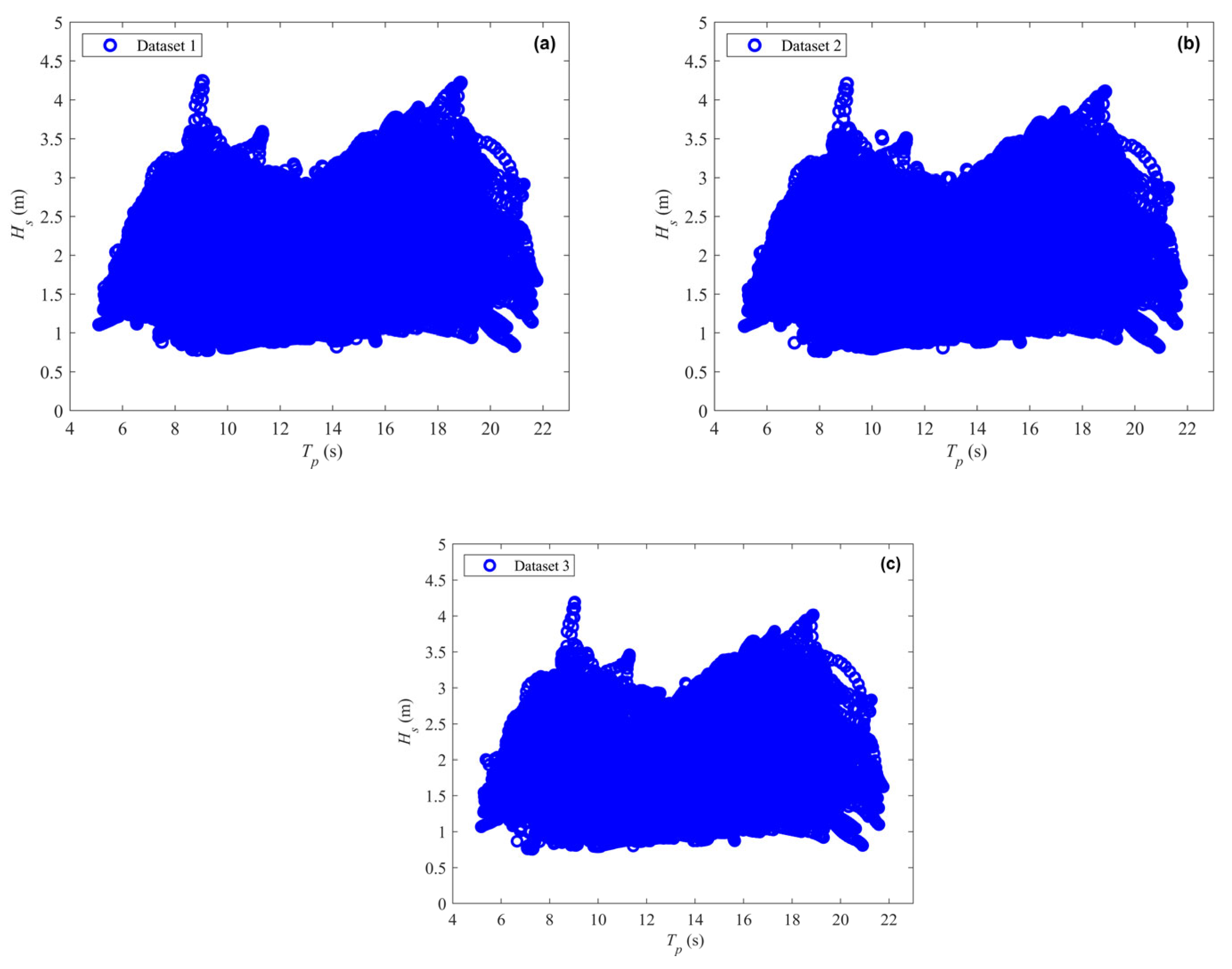
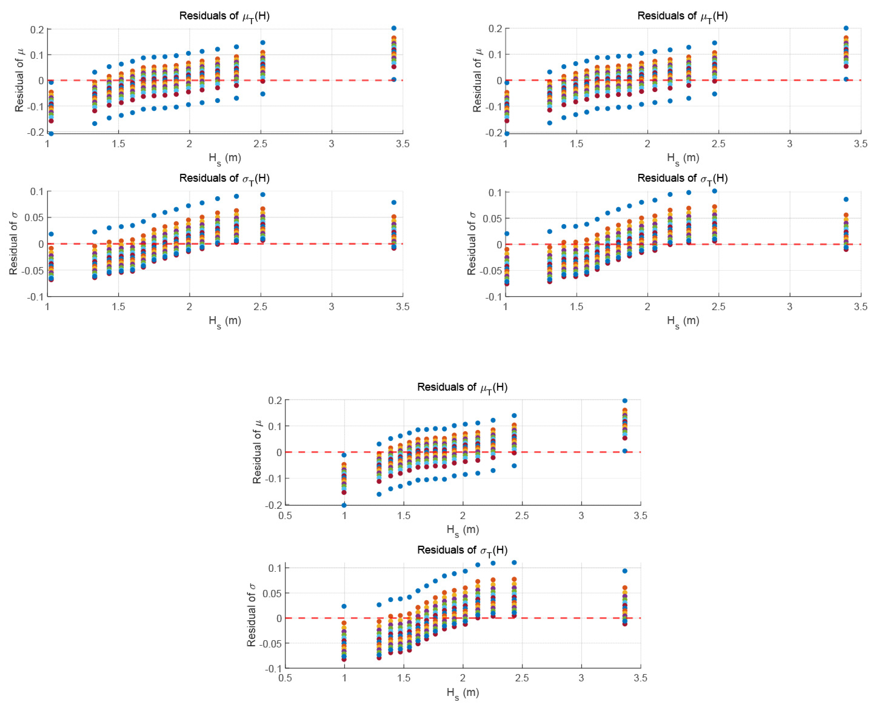
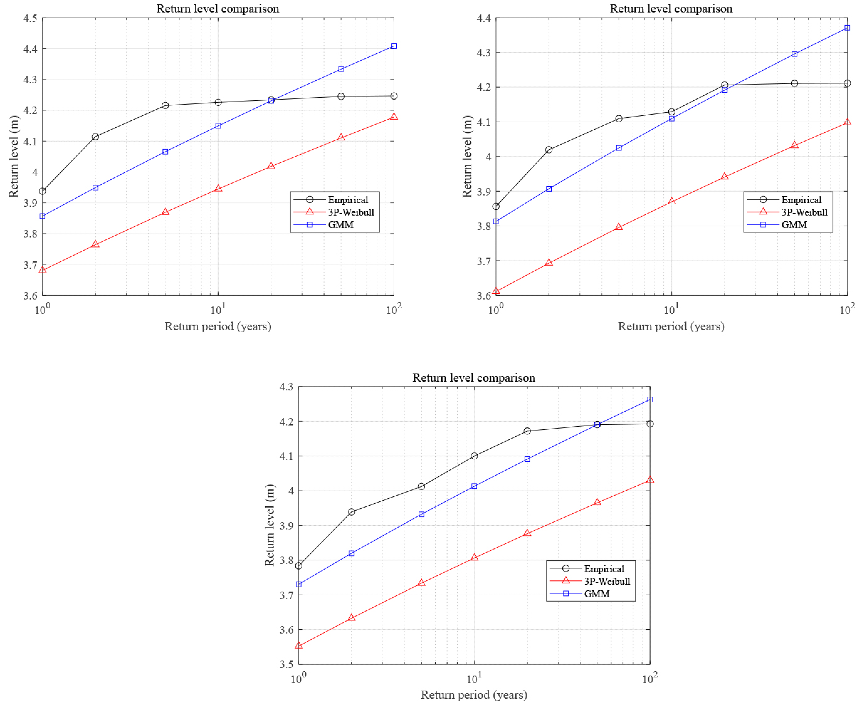
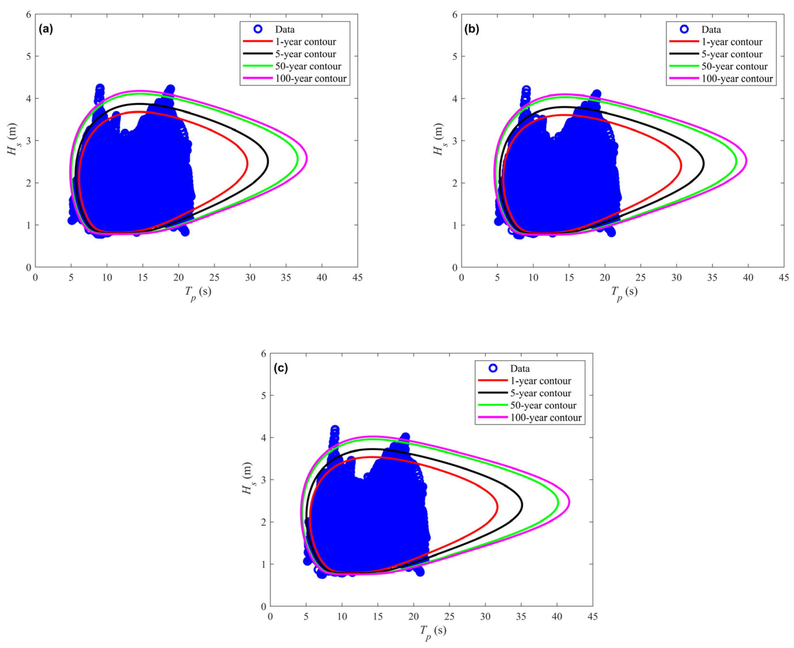
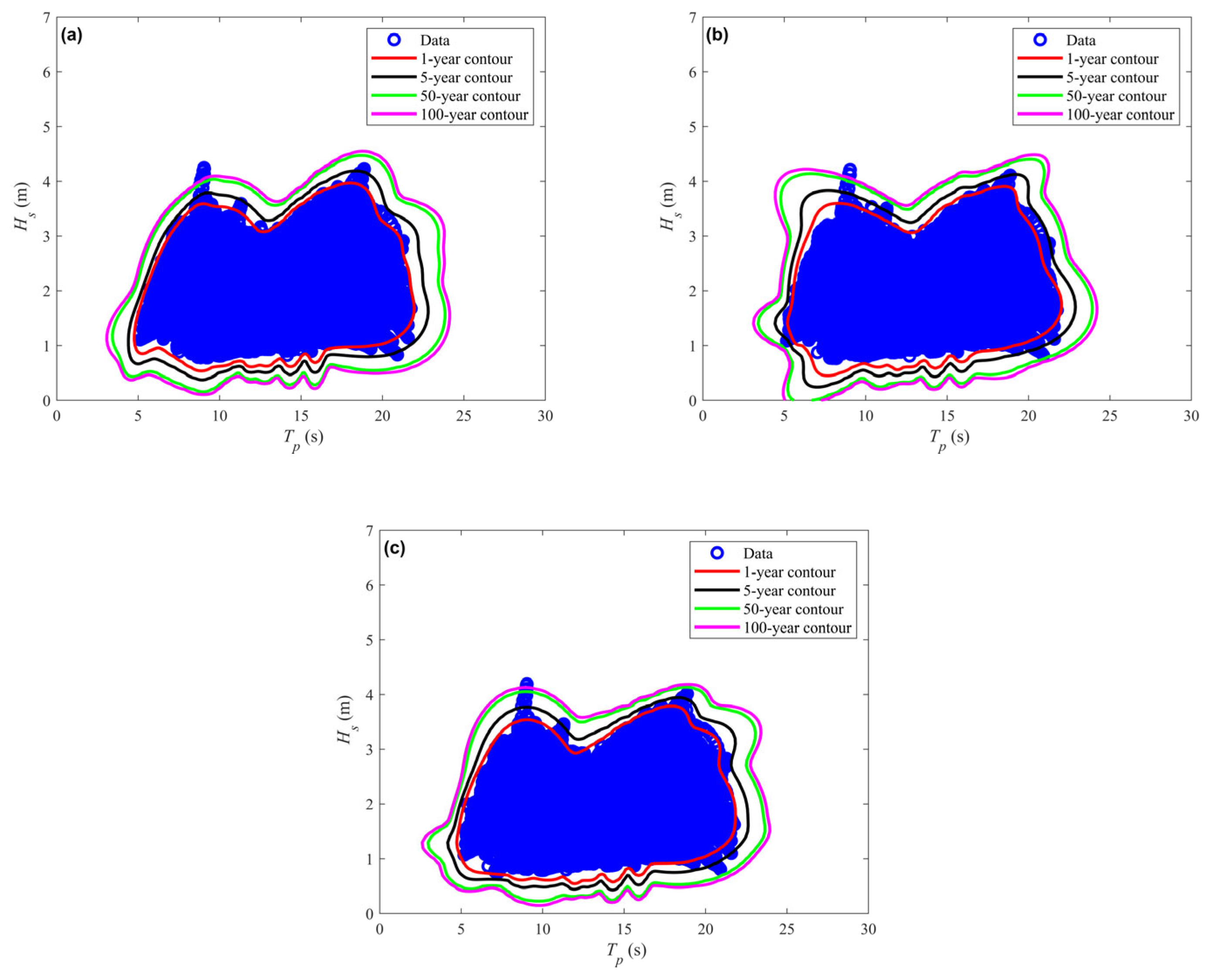
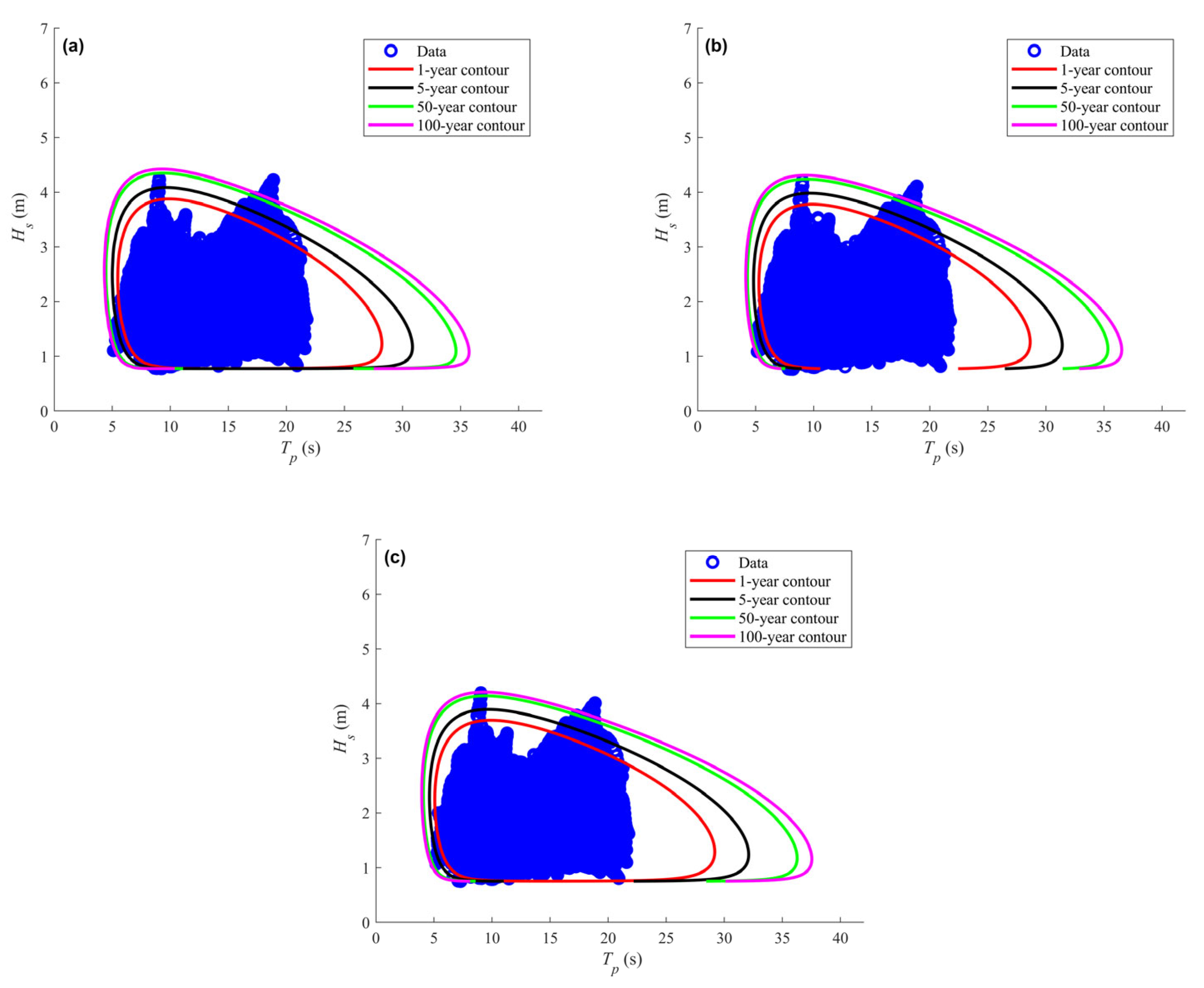
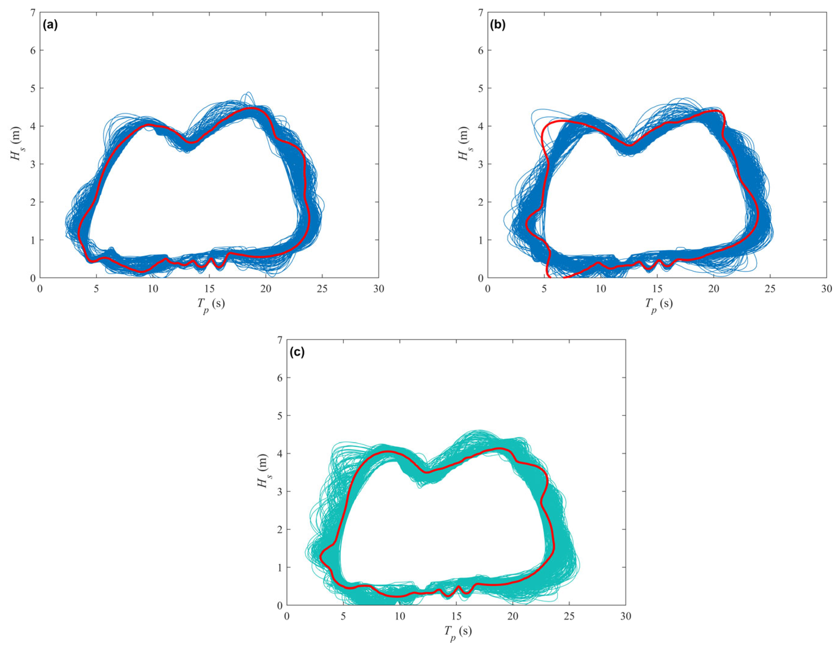
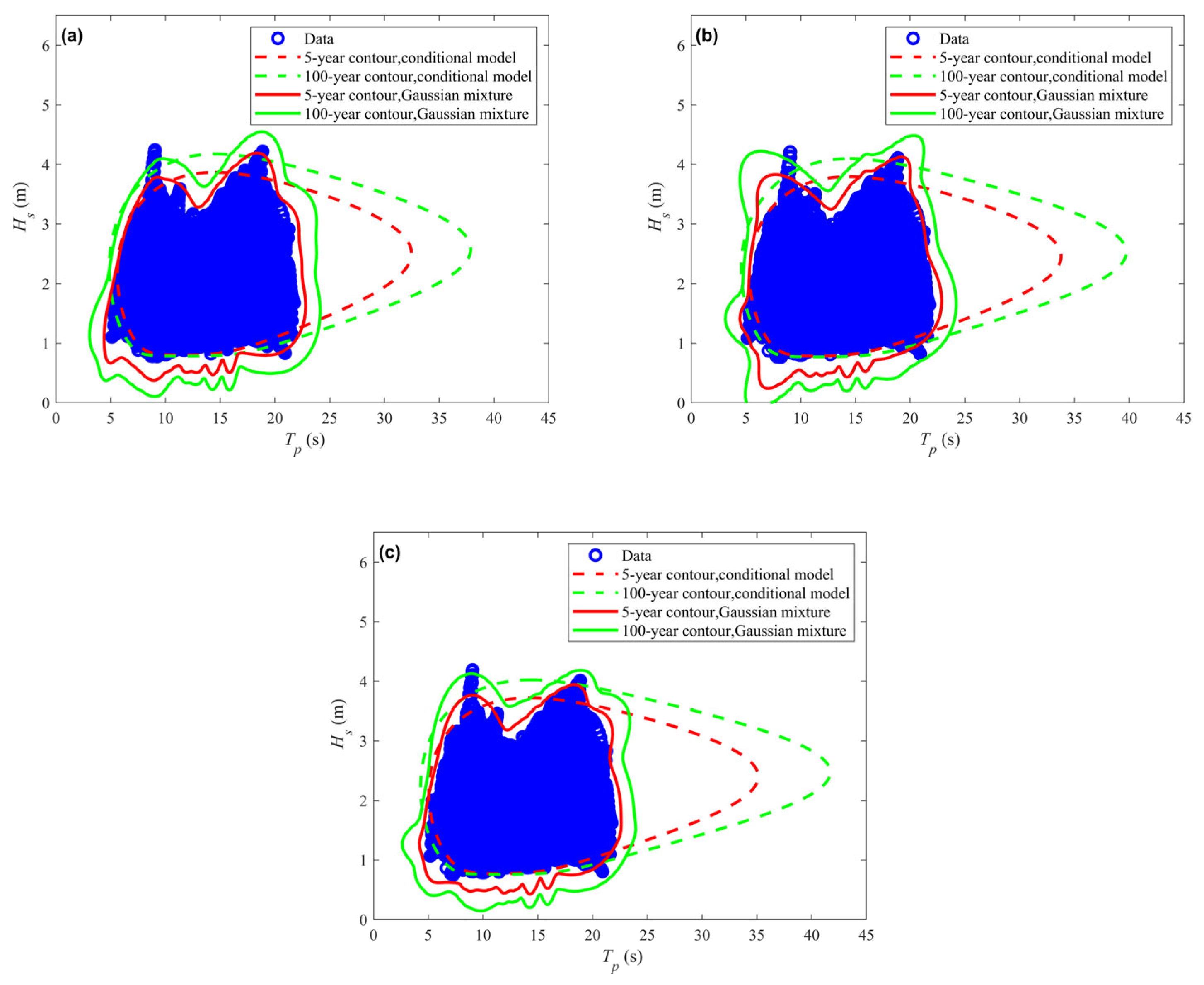
The performances of the conditional joint distribution and the Gaussian mixture distribution are further evaluated by comparing simulated data with the original observations. To facilitate this comparison, random variables are generated following the candidate joint probability density functions. Monte Carlo simulation is employed to produce discrete random wave data, and the inverse transform method is applied for random variable simulation, given that the marginal and joint distributions of the wave parameters are properly defined. For reproducibility, the random seed was fixed to 42 (
rng(42)). Initially, 100,000 uniformly distributed random samples (
z1,
z2) are generated. We repeated the simulation with 10,000, 50,000, 100,000, and 500,000 samples. The tail statistics (e.g., the 95th percentile of
Hs) showed a relative change of less than 2% when increasing the sample size from 100,000 to 500,000. Subsequently, random environmental variables are transformed as
and
for the conditional model, while for the GMM, random samples are drawn directly from the fitted mixture distribution using the
random method. For all three locations, every generated sample fell within the physically admissible range (
Hs > 0,
Tp > 0), and a sensitivity analysis confirmed that 100,000 samples provide stable tail statistics (relative change < 2% compared to 500,000 samples). In the Monte Carlo simulation, we sampled directly from the fitted GMM without explicit truncation. Given that environmental contours focus on extreme sea states (large
Hs and
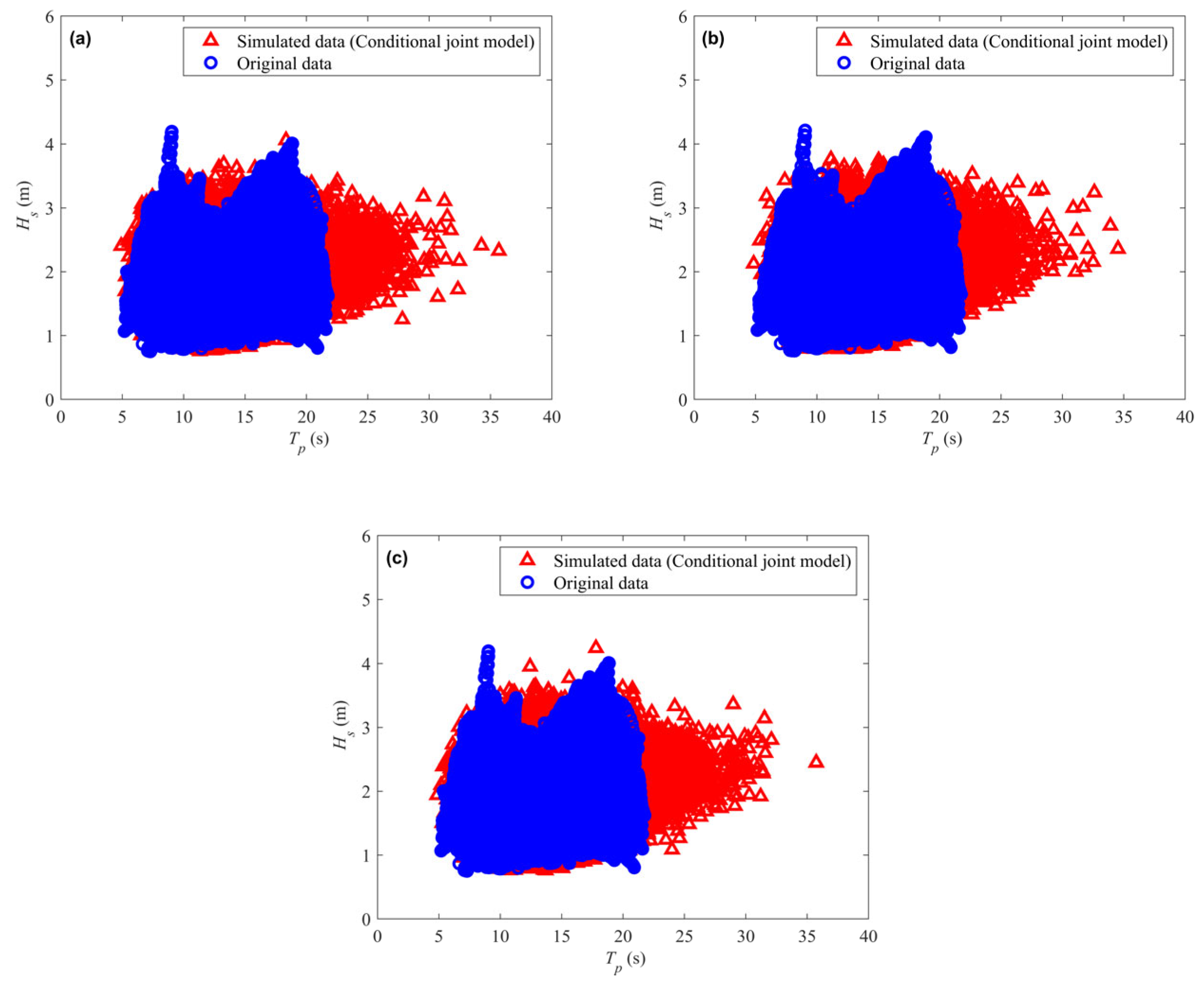
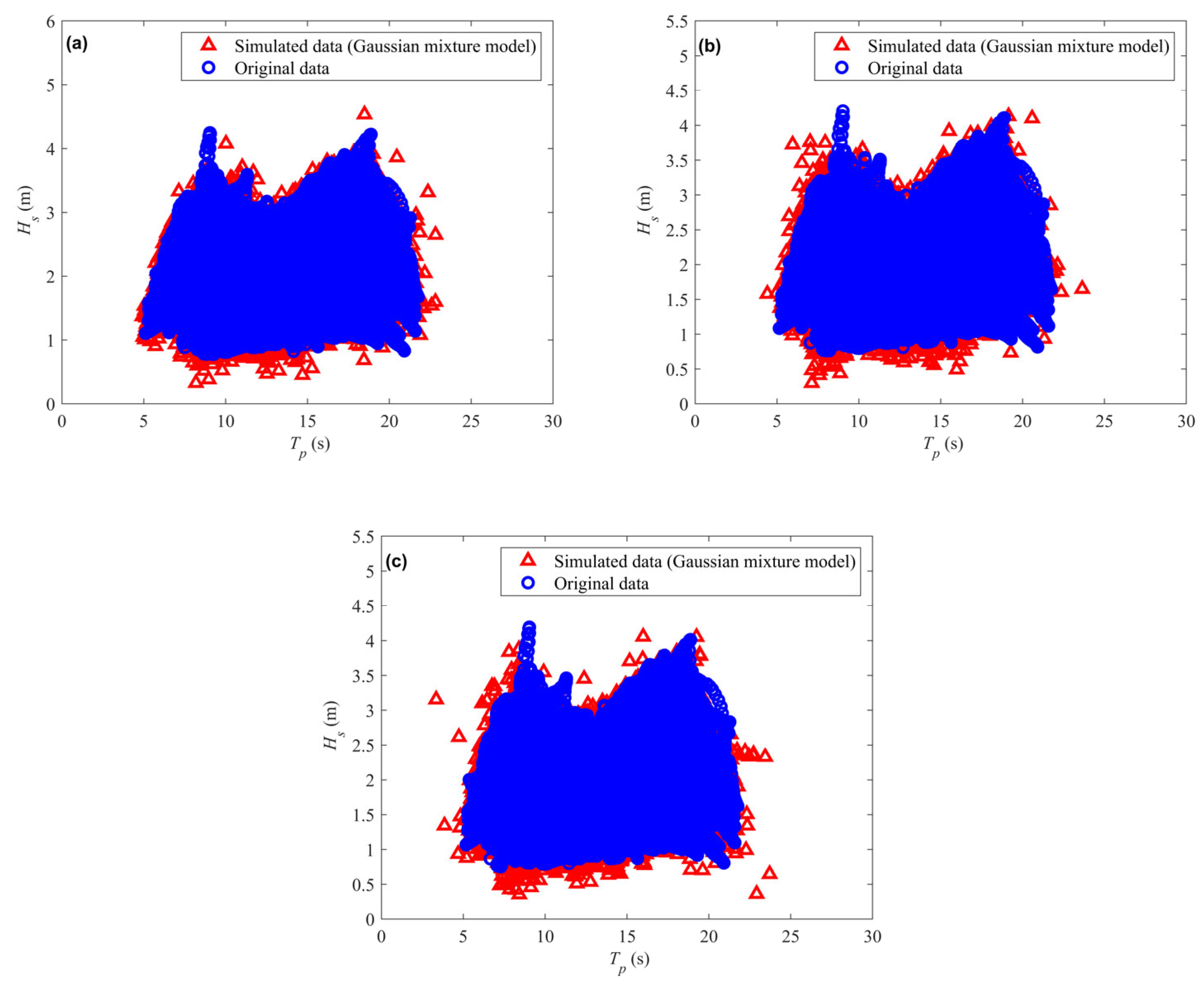
Tp), this negligible negative tail has no practical effect on the contour estimates. Therefore, we treated the negative probability mass as numerically negligible and did not apply truncation in the sampling step. Scatter plots of the original observations and simulated realizations from the conditional joint distribution and GMM are presented in
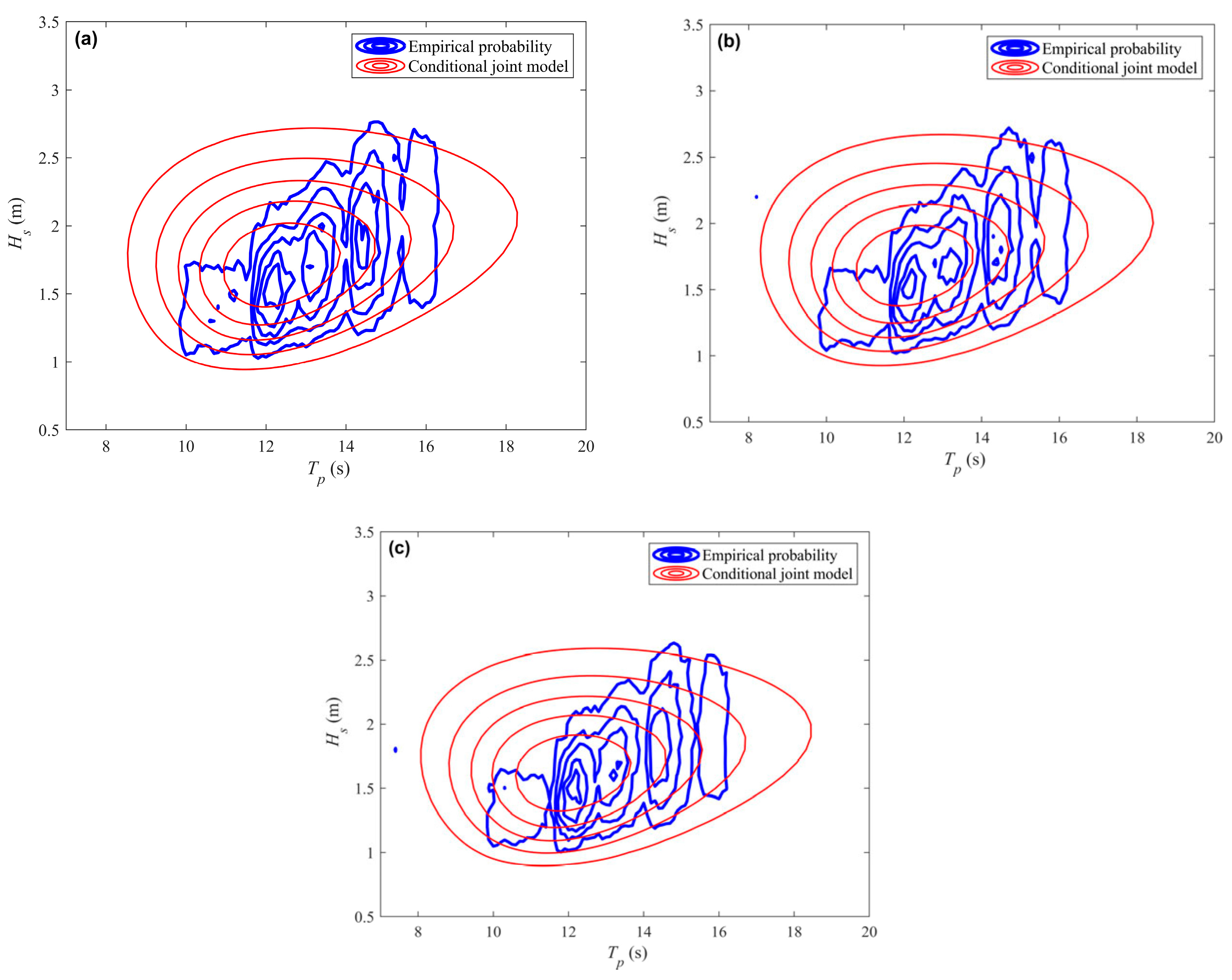
Figure 15 and
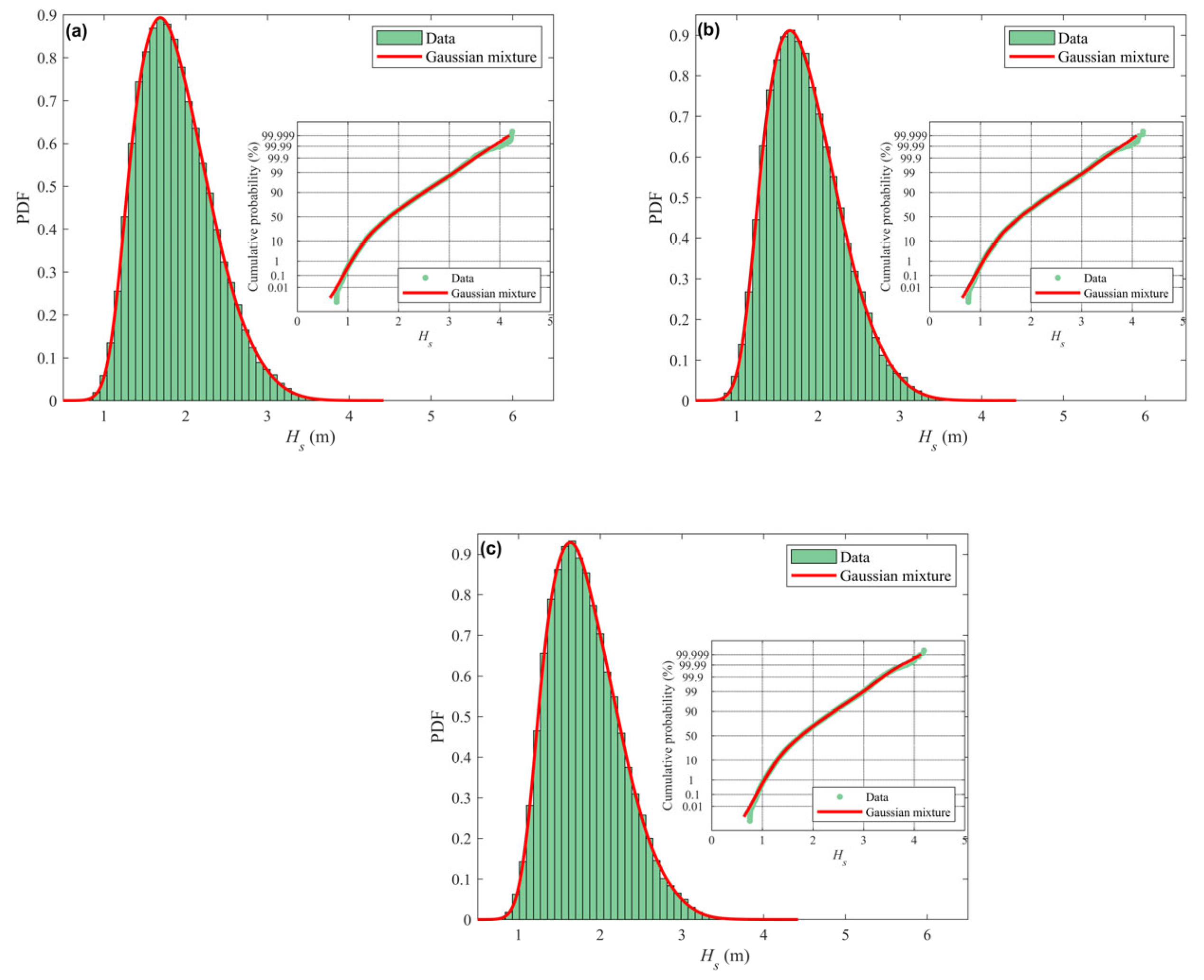
Figure 16, respectively, providing a visual assessment of the fitness of various joint models to the measured data. As can be observed from
Figure 16, the GMM yields reasonable simulations that exhibit good agreement with the empirical data across the entire range of wave conditions. The simulated data points effectively replicate the joint distribution characteristics of the original observations, including the multimodal structure and the extended tail behavior observed at all three locations. In contrast, as shown in
Figure 15, the simulated variables from the conditional joint distribution fail to fully describe the entire original dataset. Considering the complex dependence structure in datasets from locations with mixed wind and swell conditions, the mixture model provides a more accurate description of the dependence compared to the conventional conditional joint model. The ability of the GMM to capture the bimodal patterns and complex dependence structures is clearly reflected in the simulated scatter plots, which closely mirror the empirical data distribution. The results of random variable simulation based on the two candidate models are consistent with the joint probability density plots shown in
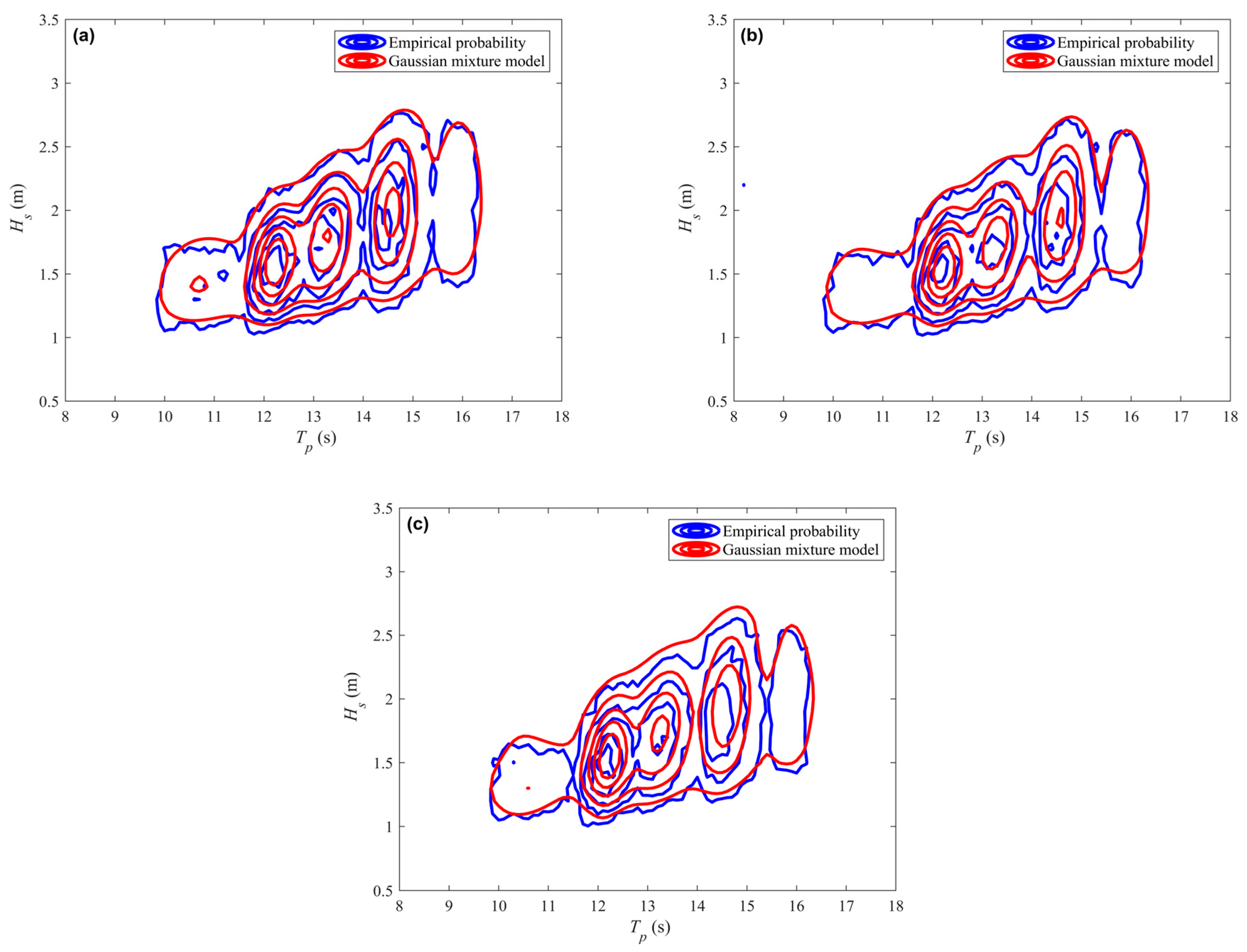
Figure 9 and
Figure 14, further validating the superior performance of the mixture model in representing both ordinary and extreme sea states.
Error Metrics
Beyond the qualitative inspection using scatter plots, a quantitative goodness-of-fit analysis was performed, and error statistics were derived to appraise the two joint probabilistic models. Two commonly adopted accuracy indicators,
RMSE and
R2, were employed to evaluate the discrepancies between empirical observations and theoretical distributions. A model with a smaller
RMSE is generally preferred, and an
R2 value approaching unity signifies a closer alignment between the measured data and model predictions.
Fi is the empirical copula value
C(
Ui,
Vi), where
Ui =
FH(
Hi) and
Vi =
FT(
Ti) are obtained via the empirical marginal distributions.
are computed from the fitted GMM and conditional models, respectively, for the GMM,
; for the conditional Weibull–Lognormal model,
.
Table 9 reports the computed error metrics. For each of the three datasets, the GMMs yield
R2 values nearly equal to 1.0000, reflecting an exceptionally strong correspondence between actual and estimated values. Clearly, the GMMs achieve markedly lower
RMSE values and therefore demonstrate a considerably better fit than their conditional counterparts. In comparison with the conditional modeling technique, the GMMs offer a substantially improved representation of the bivariate behavior of wave parameters. The RMSE values computed over the upper 5%, 10%, 15%, and 20% of the data are listed in
Table 10. Additionally, a hold-out validation (70% training/30% testing) was performed to reassess the models on independent data. The RMSE and
R2 were recomputed on the testing set using the same empirical CDF definition, and the log-likelihood values on the testing set are presented in
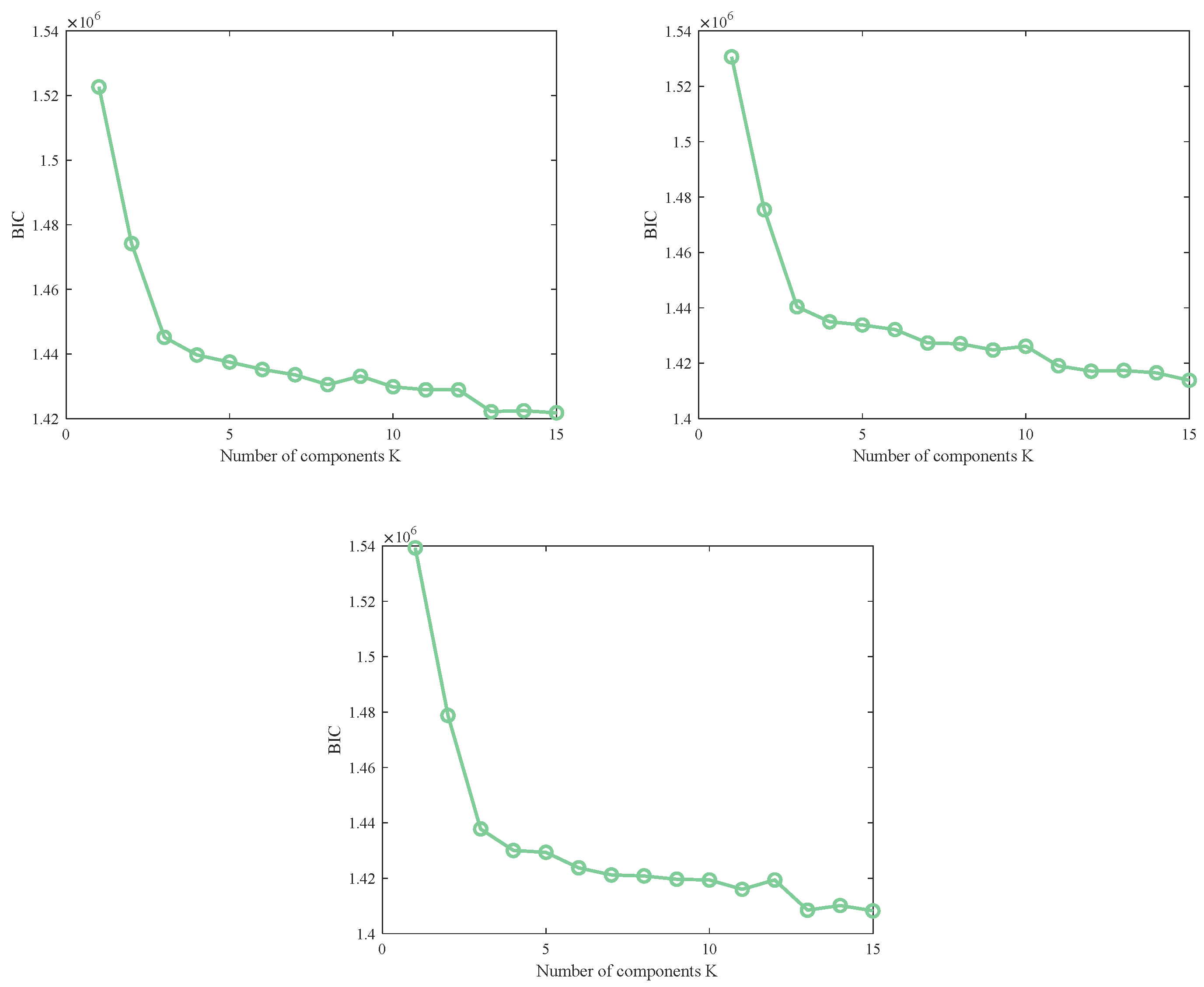
Table 11. We have performed 5-fold cross-validation for the GMM fitting. Specifically, each dataset was randomly split into five folds; four folds were used for training (EM algorithm with BIC-selected number of components) and the remaining fold for testing. This process was repeated five times, ensuring that every data point appears once in the test set. The average test-set log-likelihood and tail RMSE (upper 10% tail) were very close to the training-set values across all folds, indicating that the relatively high number of components (K = 14–15) captures genuine structure rather than overfitting noise. Detailed per-fold results are presented in
Table 12.
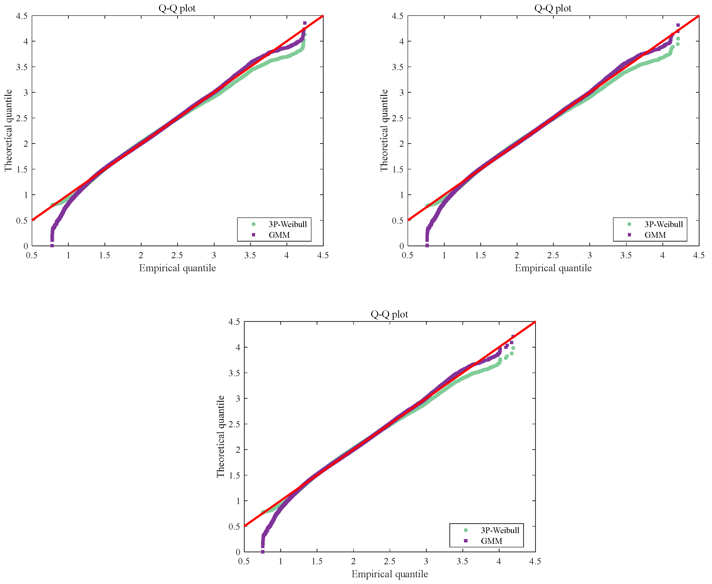
The accurate modeling of marginal distributions for significant wave height is critical, as it directly indicates the severity of sea states, especially for extreme sea condition estimation. To evaluate the performance of the adopted models, the three-parameter Weibull distribution and the GMM, univariate goodness-of-fit tests were conducted using both the KS and chi-square criteria. The test is performed using MATLAB’s built-in
chi2gof function, which automatically divides the data into a number of bins (chosen to be equiprobable under the fitted distribution) and applies a default binning strategy that ensures an expected count of at least 5 in each bin; the actual number of bins is printed in the output. The degrees of freedom are automatically corrected as df = number of bins−1−number of estimated parameters. For Dataset 2, the GMM gave a χ
2 statistic of 16.31 with df = 9, which corresponds to a
p-value of approximately 0.06. Since this
p-value is greater than 0.05, the null hypothesis (that the data come from the fitted GMM) cannot be rejected at the 5% significance level. The conditional model, by contrast, gave a χ
2 of 4.87 × 10
3 with a
p-value < 0.001, leading to rejection of the null hypothesis and indicating a clearly worse fit. To assess sensitivity to binning, we repeated the test with 8, 10, and 12 manually specified bins; the
p-value for the GMM remained above 0.05 in all cases, confirming the robustness of the GMM fit.
Table 13 summarizes the resulting statistics for the three datasets. In this table, an “(F)” mark denotes that the test statistic exceeds the corresponding critical value, implying that the theoretical distribution fails the GOF test. For all three datasets, the three-parameter Weibull distribution exhibits KS values (0.0255, 0.0272, 0.0332) larger than the critical value (0.0026) and χ
2 values (4.66 × 10
3, 4.87 × 10
3, 5.71 × 10
3) far above the respective thresholds (15.51), thus failing every test. In contrast, the GMM yields KS statistics (0.0010, 0.0015, 0.0011) below the critical value and χ
2 statistics (13.63, 16.31, 13.65) under the critical values (16.92 for all three, given 9 degrees of freedom), thereby passing all GOF tests. It is worth noting that the extremely small KS critical value arises from the large sample sizes, making the test stringent. These results indicate that the measured significant wave height records are not well represented by the conventional three-parameter Weibull distribution; its use could introduce substantial statistical errors in fitting Hs and subsequently in estimating extreme wave loads. From the perspective of both the KS and χ
2 tests, the GMM offers a superior and reliable fit for the marginal distribution of
Hs.