Wave–Current Force Characteristics of Monopile Foundations on Scoured Seabeds

Abstract

Local scour around offshore wind turbine foundations is a common engineering challenge. It changes the hydrodynamic loads and affects the foundation’s load-bearing capacity. This study investigates the field scour characteristics and wave–current force characteristics under local scour effects using field data, physical modeling, and numerical simulations. The results show that the field scour hole slope is more gradual than that observed in laboratory settings, and Zhang’s scour depth equation proves more accurate for practical engineering. In addition, under wave–current conditions (Keulegan–Carpenter number, 2 < KC ≤ 15), the relative maximum post-scour wave–current force increases with the relative post-scour water depth but decreases as the KC rises. An equation is developed to predict the relative maximum post-scour wave–current force. This provides key insights for improving load assessments of offshore wind foundations on scoured seabeds.

1. Introduction

Offshore wind power, as a burgeoning sector within clean energy engineering, presents significant potential for development and extensive application opportunities. In recent years, propelled by rapid advancements in marine construction technology, both the number and scale of offshore wind power projects have demonstrated a marked trend of accelerated growth. Nonetheless, the complex dynamics of marine environments impose substantial local scour [1,2] challenges on the foundations of offshore wind turbines. This scour phenomenon not only modifies the load distribution on wind turbine foundations but can also lead to considerable reductions in their structural bearing capacity, thereby posing serious threats to the safe and stable operation of these projects [3,4]. As a result, the issue of local scour affecting wind turbine foundations, along with the associated variations in load, has persistently been a focal point of research and concern among engineers and scientists.

Many scholars have conducted extensive research on local scour related to wind turbine foundations. These studies, conducted under varying hydrodynamic conditions, can be categorized into three primary types: unidirectional current, wave [5] or wave–current, and tidal current. Under unidirectional currents, numerous studies [6,7,8] have demonstrated that local scour at piles progresses rapidly during the initial phase, eventually reaching a static or dynamic equilibrium. The ultimate equilibrium scour depth is influenced by factors such as flow velocity, water depth, sediment characteristics, and the dimensions of the pile foundation. Using relevant empirical investigations, various scholars have developed distinct methodologies for calculating local scour depth. Notable examples include the US HEC-18 equation [9], Melville’s method [10], the Ettmer equation [11], and the cohesive soil standard equation [12], among others. As for wave or wave–current conditions, Sumer and Fredsøe [13,14] studied the scour mechanisms of large-diameter piles under wave or wave–current conditions. They argued that the KC number is the main factor influencing scour depth under pure wave action, while under wave–current combined action, the current velocity ratio is also a key factor affecting scour depth in addition to the KC number. Qi et al. [15] investigated the equilibrium scour depth around pile foundations under wave–current conditions using a physical model and formulated a scour equation related to the wave–current Froude number (Fr_a). Guan et al. [16] established a machine learning model to predict local scour depth under wave or wave–current conditions. Under tidal conditions, flow velocity changes periodically with bidirectional flow directions. A tidal cycle is often semi-diurnal [17], with a longer period and gentler velocity change than waves. These conditions cause complex vortex systems to alternate around pile foundations, impacting local scour development. Some scholars [18,19,20,21,22] have used experiments and simulations to study scour under tidal currents. They found that scour depths are typically less than those under steady flows. However, scale effects limit these findings, causing discrepancies with real-world scour patterns. Recent advancements in field observation technologies have provided new insights from offshore wind projects or sea-crossing bridge. Several researchers [23,24,25,26] have conducted analyses on the collected field scour data, revealing significant discrepancies between field scour depth and present scour equations. Zhang et al. [20] analyzed the geometry and depth characteristics of the scour hole using field data from the Hangzhou Bay Bridge. The results showed that the field scour slopes under tidal currents are gentler than the angle of repose. In addition, the scour depths are similar to those under steady flows at high intensities but differ significantly at low intensities. In conclusion, the scale effects result in discrepancies between the characteristics of scour holes observed in real-world engineering projects and those derived from laboratory experiments. With the growing availability of field observation data, it is imperative to conduct analyses of the morphological characteristics of scour holes in practical engineering contexts using extensive empirical data. Furthermore, assessing the applicability of existing scour equations to actual engineering conditions is essential. Despite this necessity, a systematic and comprehensive study has yet to be undertaken.

In the study of wave or wave–current loading on monopiles, the Morison equation (Equations (1) and (2)) [27] represents the most widely utilized theoretical framework.

$$f={\displaystyle \frac{\rho C_{D}D}{2}}[u(z,t)+u_0]\left|u(z,t)+u_0\right|+{\displaystyle \frac{\rho C_M\pi D^2}{4}}\left({\displaystyle \frac{\partial u(z,t)}{\partial t}}\right)$$

(1)

$$F={\int }_{-h_0}^{\eta \left(t\right)}fdz$$

(2)

where f is the wave–current force per unit length at elevation z; D is the diameter of the mono pile; u(z,t) is wave velocity at elevation z and u₀ is current velocity; h₀ is stationary water depth; η is water surface elevation; and F is the total wave–current force of the monopile. C_D and C_M are the drag coefficient and inertia coefficient, respectively.

Morison theory disaggregates wave–current forces into two components: drag force and inertia force. As shown in Equations (1) and (2), the drag component scales with the square of the wave orbital velocity or the combined wave and current velocity, while the inertial component scales linearly with wave acceleration. Extensive research [28,29,30,31] has been conducted by numerous scholars on the drag coefficient C_D and inertia coefficient C_M within the Morison equation, with pertinent design codes providing guidelines for these parameters. Their studies reveal that both coefficients correlate with the KC [31] under both pure wave and combined wave–current conditions.

$$KC=\left\{\begin{array}{c}{\displaystyle \frac{U_{m}T}{D}}[\sin \phi +\left(\pi -\phi \right)\cos \phi , u_m>u_0\\ {\displaystyle \frac{\pi u_{0}T}{D}}, { u}_m\le u_0\end{array}\right.$$

(3)

where u_m is the maximum wave velocity at stationary water depth $\phi ={\cos }^{-1}(u_0/u_m)$.

Specifically, C_D exhibits an initial increase followed by a subsequent decrease with increasing KC, whereas C_M decreases monotonically with KC and gradually asymptotes to a stable value. Nevertheless, existing studies have predominantly concentrated on scenarios involving a horizontal seabed surface. In practical engineering, however, the presence of a local scour hole modifies the local flow regime and increases the exposed length of the pile, rendering the conventional Morison method inadequate. Some researchers have explored the impact of wave–current loading under scour conditions, contributing to the understanding of these complex interactions. For instance, Sui et al. [32] conducted an investigation into the dynamic response of wave–seabed interactions in the presence of scour holes, concluding that the pile loading experienced an increase. Similarly, Li et al. [33] examined the dynamic response of wave interactions on a monopile foundation on a scoured seabed and also reported an increase in loading. As for the steady current condition [34], the presence of a scour hole leads to substantial attenuation or even the disappearance of wake vortex structures. This flow regime causes the flow field around the pile to become increasingly streamlined, transforming the pressure distribution in the downstream region at the pile base from negative to positive pressure. Consequently, the total hydrodynamic load on the pile decreases compared to the flat seabed condition. As noted in a previous study, the influence of scour on hydrodynamic loads differs between pure wave action and pure current action. Moreover, under coupled wave–current action, the interaction between waves and currents complicates the composition of inertial and drag forces, thereby influencing the variation in wave–current forces under scour conditions. Given this intricate force composition, the specific influence of factors such as KC or wave height on wave–current forces under scour conditions, independent of scour depth effects, has yet to be elucidated.

This study aims to achieve a comprehensive understanding of the wave–current hydrodynamic response of offshore wind monopiles on scoured seabed. Based on field data from various offshore projects, the research evaluates the morphology and characteristics of scour holes. Furthermore, a combined approach of physical experimentation and numerical simulation is employed to investigate the hydrodynamic performance under wave–current conditions on both flat and scoured seabeds.

2. Methods

2.1. Field Scour Data

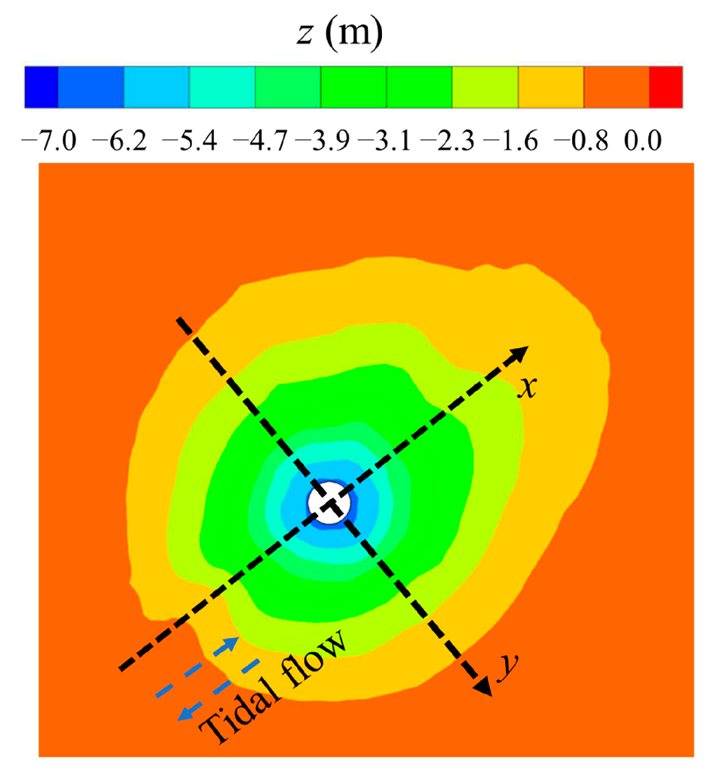
In the analysis of scour holes, the primary focus is on both scour depth and profile. Figure 1 illustrates the typical geometry of a scour hole as observed in practical engineering. To investigate prototype-scale scour characteristics, this study compiled field data from several offshore wind farms (OWFs). These data cover scour under combined wave and tidal current conditions, which are prevalent in practical engineering. In addition, field data from several sea-crossing bridge projects are also collected. The sources of these field measurements are detailed in

Table 1. Statics of field scour data.

No	Site	Sediment Median Diameter (mm)	Annual Mean Significant Wave Height (m)	Peak Tidal Current (m/s)	Mean Water Depth (m)	Pile Diameter (m)	Scour Depth (m)	References
1	Scroby Sands OWF, UK	0.26	1.0	1.10	7.5	4.20	5.80	[23]
2	N7, North Sea, The Netherlands	0.20	1.1	0.75	7.0	6.00	6.30	[25]
3	Scarweather Sands OWF, UK	0.28	1.4	1.10	11.0	2.20	2.50	[25]
4	Destin tidal inlet bridge pier, USA	0.28	0.0	0.60	3.8	0.86	1.10	[25]
5	Barrow OWF, UK	0.22	1.2	0.80	15.0	4.75	5.75	[25]
6	Otzumer Balje inlet bridge, Germany	0.36	0.0	1.40	11.7	1.50	2.20	[25]
7	Gunfleet Sands OWF, UK	0.20	1.6	1.10	11.4	4.70	8.00	[26]
8	Robin Rigg OWF, UK	0.25	1.2	1.60	9.0	4.50	7.60	[24]
9	Dafeng OWF, China	0.02	0.8	1.66	20.0	7.25	8.00	[35]
10	Hangzhou Bay bridge, China	0.05	0.5	2.89	13.2	4.06	10.10	[20]
11	Xiangshan bridge, China	0.004	0.5	1.50	18.6	8.00	1.90	[20]

. The field data encompass seabed environments composed of both non-cohesive sand (d₅₀ > 0.08 mm) and cohesive silt (d₅₀ < 0.005 mm). Furthermore, the peak current velocity during a typical spring tide and the annual mean significant wave height are utilized as hydrodynamic conditions in this study given that scour development is a long-term process. A spring tide cycle has an approximate duration of 12 h. With approximately 24 spring tides occurring each year, the cumulative duration extends to 24 days. In contrast, the period during which the annual maximum significant wave height occurs is generally limited to a few hours, which is inadequate to achieve equilibrium scour. Therefore, the annual mean significant wave height is chosen as the representative wave height for this analysis.

2.2. Experiment Setup

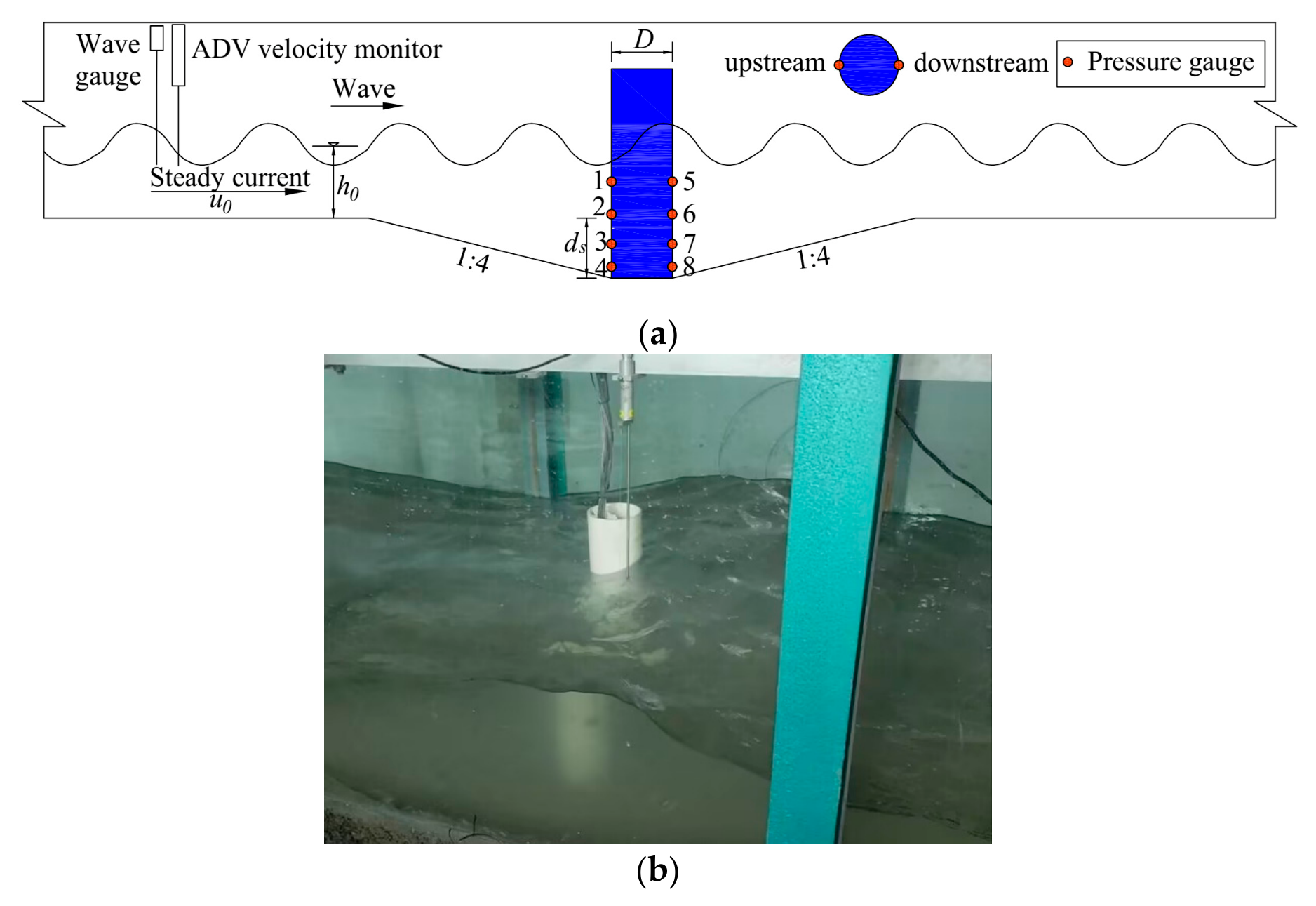
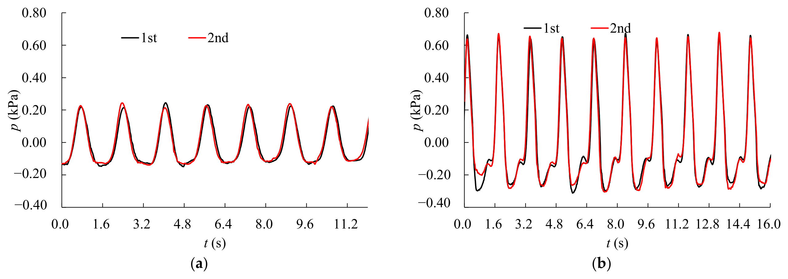
The wave–current forces on monopile foundations are investigated through a combined experimental–numerical approach. The experiments were conducted in the wave–current flume at the Zhejiang Institute of Hydraulics and Estuary, Hangzhou, China. The flume is 50 m in length, 1.5 m in width, and 1.2 m in height. The comprehensive experimental setup is depicted in Figure 2. The monopile model, constructed from a cylindrical plastic pipe with a diameter of 0.11 m, was centrally positioned in the flume, approximately 27 m from the wave generator. Two wave gauge were respectively placed 2 m upstream of the pile and at the position of pile. An acoustic Doppler velocimeter (ADV) (Nortek, Rud, Norway) was installed to measure current velocity. Both flat bed and scoured bed conditions were systematically examined. In the scoured bed scenario, a single scour depth of (d_s = 0.15 m) was examined. It has a side slope ratio of 1:4, which is close to the scour slope in practical engineering. Eight pressure sensors were strategically installed on the model pile, with four sensors positioned on the upstream face and four on the downstream face. The specific positions of each pressure sensor are detailed in

Table 2. Distribution of pressure gauges.

z (m)	Pressure Gauge No.
	Upstream	Downstream
0.10	1	5
0.02	2	6
−0.06	3	7
−0.14	4	8

. It should be noted that, under the flat bed condition, only sensors numbered 1, 2, 5, and 6 are capable of recording pressure data. A total of 32 experimental runs are conducted, with wave height varying from 0.04 m to 0.10 m and flow velocity reaching up to 0.33 m/s. According to Equation (3), the KC of experimental cases ranges from 2 to 15. The comprehensive test parameters are outlined in

Table 3. Experimental cases.

Seabed Type	Water Depth h0 (m)	Time Period T (s)	Wave Height H (m)	Current Velocity u0 (m/s)
Flat seabed	0.22	1.64	0.04, 0.06, 0.08, 0.10	0, 0.11, 0.22, 0.33
Scoured seabed	0.22	1.64	0.04, 0.06, 0.08, 0.10	0, 0.11, 0.22, 0.33

. Duplicate tests were also conducted for each case. Figure 3 illustrates the consistency of the time history of pressure at Gauge No. 1 under wave heights of 0.04 m and 0.10 m with steady current u₀ = 0.33 m/s. The pressure variation processes for the two tests under each case demonstrate a high degree of concordance. Statistically, the mean discrepancy between the two measurements is approximately 0.001 kPa, with a maximum discrepancy of about 0.006 kPa, both of which are below 0.01 kPa. The repeatability deviation is less than 3% of the maximum pressure, signifying a high level of repeatability.

2.3. Numerical Model

The olaFlow solver within the OpenFOAM framework is selected for modeling wave–current hydrodynamics. This solver resolves the incompressible Navier–Stokes equations, employing the volume of fluid (VOF) method to capture wave free surfaces. The governing equations, expressed in differential form, are as follows:

$${\displaystyle \frac{\partial u_i}{\partial x_j}}=0$$

(4)

$$\rho {\displaystyle \frac{\partial u_i}{\partial t}}+\rho u_j{\displaystyle \frac{\partial u_i}{\partial x_j}}=-{\displaystyle \frac{\partial p}{\partial x_i}}+{\displaystyle \frac{\partial }{\partial x_j}}\left(\mu {\displaystyle \frac{\partial u_i}{\partial x_j}}\right)+s_i$$

(5)

where u is the velocity vector; s the source term; subscripts i and j (=1, 2, 3) represent the x, y, and z directional components; p is the pressure; ρ is the density; and μ is the dynamic viscosity.

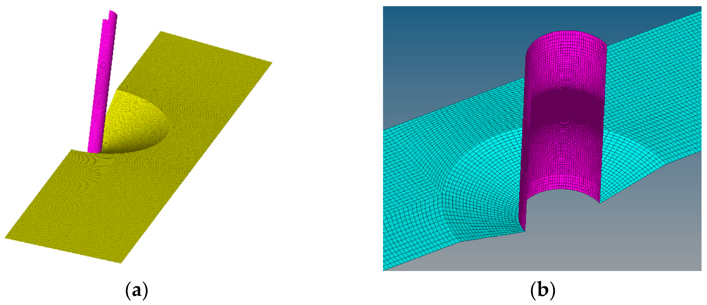
In the numerical simulations, the computational domain is configured with a length of 13 m, and the cylindrical pile, with a diameter of 0.11 m, is positioned at x = 6.5 m to align with the parameters of the physical experiments. Due to the symmetry inherent in the structure and flow field, only half of the structure is modeled to optimize computational efficiency. The width of the flume is set at 1.0 m. To ensure computational precision, local mesh refinement is implemented near the cylinder and the free surface. In the horizontal plane, the mesh size varies from a maximum of 0.03 m to a minimum of 0.005 m. In the vertical (z) direction, it ranged from a maximum of 0.005 m to a minimum of 0.002 m. The simulations encompassed all cases from the physical experiments, including both flat bed and scoured bed conditions. Moreover, simulations are also carried out for the conditions of h₀ = 0.15 m, H = 0.06 m, and u₀ = 0.33 m/s current velocity on both flat and scoured beds. Figure 4 provides an illustration of the computational domain and local mesh configuration for the scoured bed scenario. In terms of boundary conditions, the left boundary of the computational domain is designated as a wave generation boundary. To mitigate the effects of wave reflection, active wave absorption boundaries are employed on both the left and right boundaries. The front wall, bottom surface, and cylinder surface are characterized as no-slip boundaries, whereas the rear boundary is defined as a symmetry boundary.

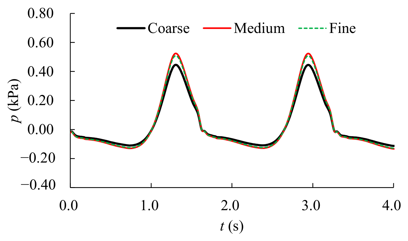
To discretize the governing equations, this work employs a first-order Euler scheme for temporal derivatives, while the Gauss linear approach is utilized for both gradient and velocity divergence terms. The Gauss interface compression method is implemented for the phase volume divergence, and a corrected Gauss linear scheme is applied to the Laplacian terms. The k-ω SST turbulence model is adopted in this study, with its detailed governing equations omitted for the sake of brevity. The convergence of each time step is controlled by residual tolerances of 10⁻⁷ for pressure and 10⁻⁸ for velocity, volume fraction, and turbulence quantities, with a maximum of 20–30 inner iterations and 3–5 PIMPLE outer correctors; the simulation proceeds only when the global continuity error falls below 10⁻⁶. For near wall turbulence, a blended wall treatment based on the SST k-ω turbulence model is employed. This approach automatically transitions between the viscous sublayer formulation and the logarithmic law of the wall according to the local dimensionless wall distance y⁺. Specifically, the wall boundary condition for a specific dissipation rate ω is prescribed using a smooth quadratic blending of the viscous sublayer solution (applicable at y⁺ < 5) and the logarithmic layer solution (applicable at y⁺ > 30). This blended formulation eliminates the requirement for the first cell centroid to be strictly located in the logarithmic layer (y⁺ = 30–300) and ensures numerical robustness across the buffer layer (5 < y⁺ < 30). The time step is automatically adjusted at each iteration to maintain a Courant number below 0.2, a conservative threshold widely adopted in transient free-surface flow simulations to ensure both numerical stability and temporal accuracy. The adaptive time step is strictly bounded between a minimum of 0.0005 s and a maximum of 0.002 s throughout the entire computation. A grid sensitivity analysis was conducted using three meshing strategies. The maximum planar mesh sizes in the upstream region of the cylinder are 0.05 m (coarse mesh), 0.03 m (medium mesh), and 0.01 m (fine mesh), respectively. Figure 5 presents the pressure variations at Gauge No. 1 (H = 0.08 m, u₀ = 0.33 m/s) under the three grids. The maximum difference between the fine and medium meshes is less than 5%. Therefore, the medium mesh is used in the following simulations.

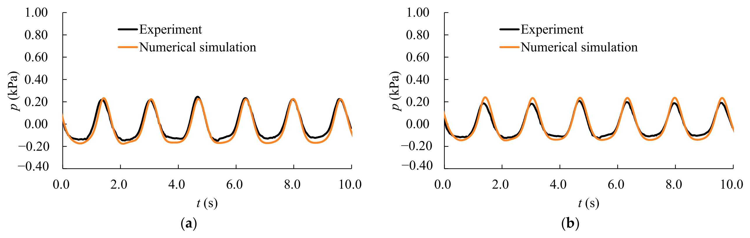
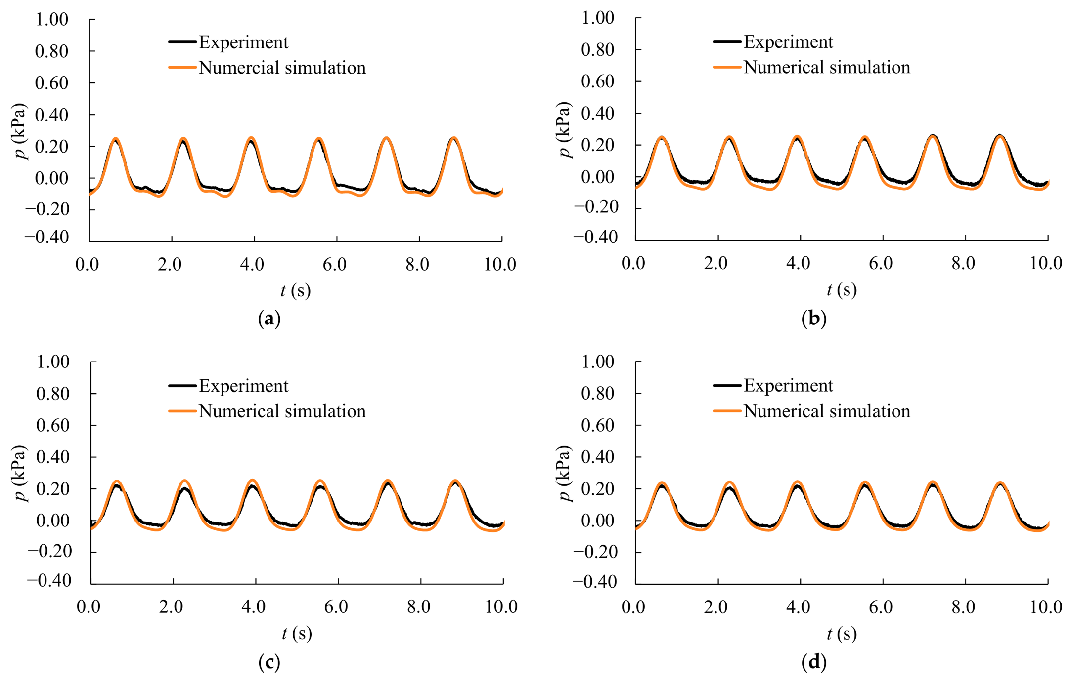
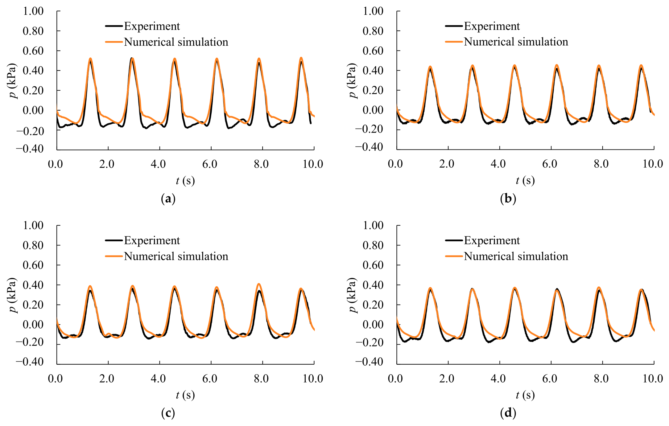
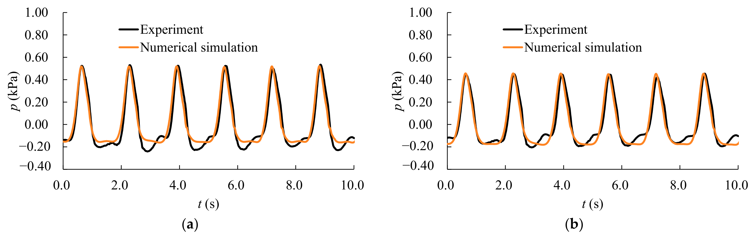
The numerical model was further validated against multiple test conditions: (1) H = 0.04 m, u₀ = 0.33 m/s, flat seabed; (2) H = 0.08 m, u₀ = 0.33 m/s, flat seabed; (3) H = 0.04 m, u₀ = 0.33 m/s, scoured seabed; and (4) H = 0.08 m, u₀ = 0.33 m/s, scoured seabed. Figure 6, Figure 7, Figure 8 and Figure 9 present the comparisons between the numerical simulation results and the physical experimental results for the different conditions. The corresponding positions of the pressure sensors are listed in Table 2. It can be observed that for both large and small wave heights, the numerical simulation results are in good agreement with the physical experimental results. The average error of the maximum pressure for each condition is within 0.03 kPa, with a relative error of approximately 6%, indicating that the numerical simulation results are basically reliable.

3. Results and Discussions

3.1. Scour Depth

Numerous predictive models have been developed to estimate equilibrium scour depth. In the context of wave–current interactions, the DNV equation and Qi equation are frequently cited. In addition, some engineers apply steady or tidal current scour equations to predict maximum scour value. The mathematical equations of above are presented below.

DNV Equation

$$d_s/D=1.3$$

(6)

where d_s denote the scour depth, and D indicates the monopile diameter.

Qi Equation [15]

$$\lg \left({\displaystyle \frac{d_s}{D}}\right)=1.11-0.8e^{\left({\displaystyle \frac{0.14}{{Fr}_a}}\right)}$$

(7)

where Fr_a is the wave–current Froude number, which is defined as $F{r}_a=u_a/\sqrt{gD}$. Here, g represents the gravitational acceleration, and u_a indicates the combined wave–current velocity. The expression for u_a is given by $u_a=u_0+2u_m/\pi$, where u₀ is the tidal current velocity, and u_m the maximum wave-induced velocity.

HEC-18 Equation [9]

$$d_s=2.0k_1{k}_2{k}_3{\left({\displaystyle \frac{D}{h}}\right)}^{0.65}{Fr}^{0.43}$$

(8)

where k₁, k₂, and k₃ are the pile type coefficient, the water flow and pier angle coefficient, and the seabed coefficient, respectively. In present study, k₁ and k₂ coefficients both equal 1.0, and k₃ is 1.1 in case of flat seabed. h represents the water depth. Fr is Froude number $Fr=u/\sqrt{gh}$.

Zhang Equation [20]

$$d_s=2.2k_1{k}_2(0.1{\displaystyle \frac{u_a}{u_c}}+0.52)D^{0.65}({\displaystyle \frac{2.6u_a-u_c}{\sqrt{g}}}{)}^{0.7}$$

(9)

where u_c denotes the sediment incipient velocity and other symbols retain their previous definitions.

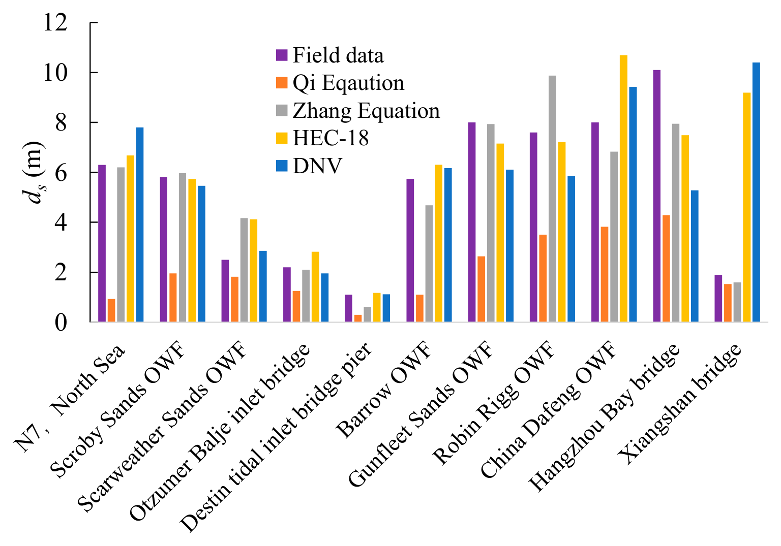
The previously mentioned scour depth equations were validated using collected field observation data. Figure 10 and

Table 4. Statics of relative errors and RMSE.

Prediction Method	Qi	Zhang	HEC	DNV
Relative error (%)	56	21	52	56
RMSE (m)	3.91	1.24	2.51	3.10

illustrate the comparison between the calculated and observed values for each equation. It is apparent that the Qi equation generally produces underestimated predictions, with a relative error of 56%, indicating that its calculated values are typically lower than the field measurements. Conversely, the Zhang equation demonstrates superior performance, with a relative error of only 21%, closely aligning with the field data and thereby exhibiting higher accuracy. The internationally recognized HEC-18 method results in a relative error of 52% and shows an overall deviation. Similarly, the DNV method yields a relative error of 56%, with predictions generally exceeding the observed values. In terms of RMSE (root mean square error), Zhang’s method stands out as the only one with values below 2 m, while all other methods yield values between 2 and 4 m. In summary, the Zhang equation achieves the highest predictive accuracy among the four methods, whereas the Qi equation and DNV method exhibit relatively lower precision.

3.2. Scour Hole Slope

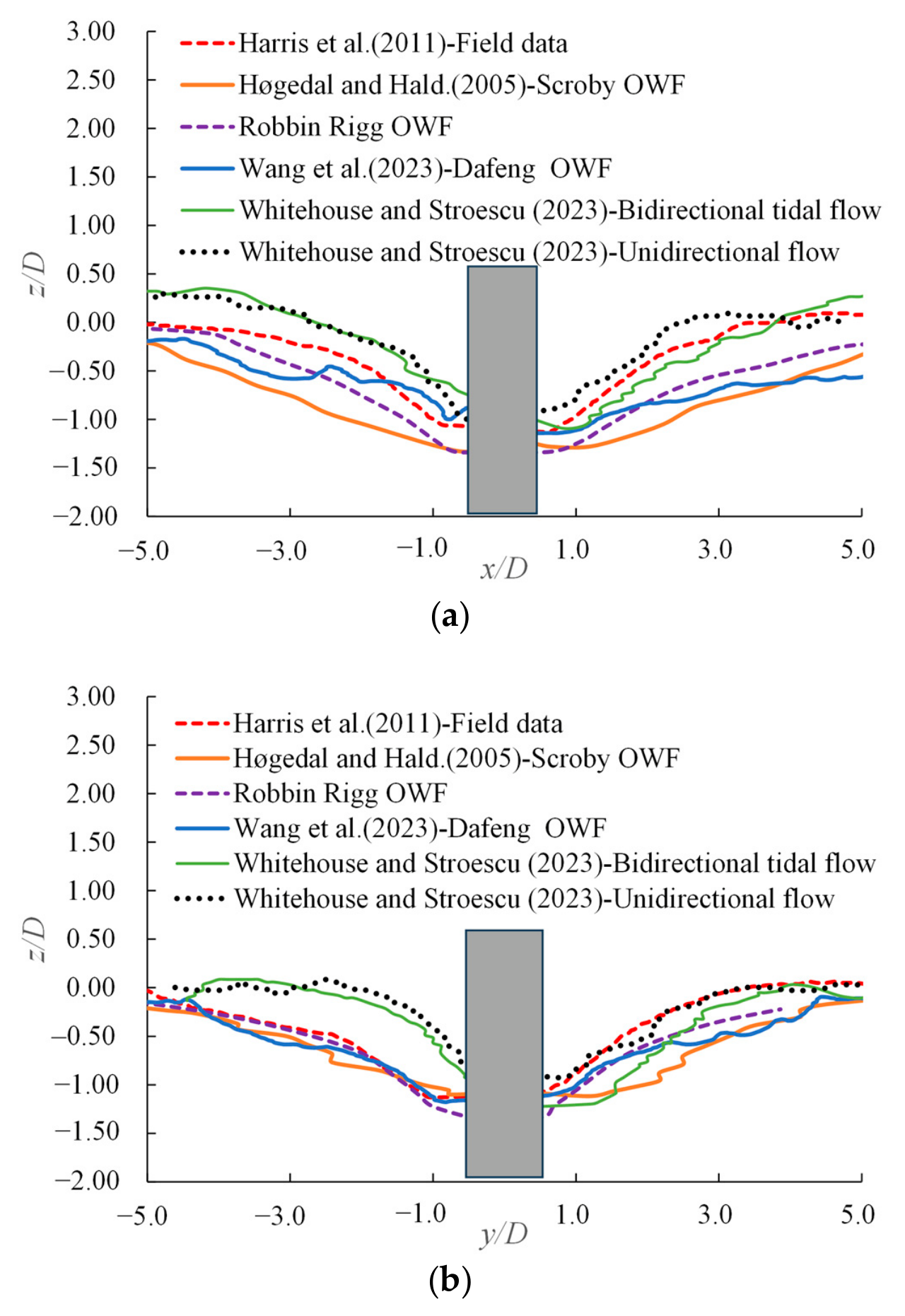
In addition to scour depth, the dimensions of the scour hole significantly affect local hydrodynamic properties. For monopile foundations, the side slope of the scour hole acts as a clear indicator of the scour profile, with gentler slopes indicating larger affected areas. Previous laboratory-scale physical experiments and numerical simulations have suggested that the side slopes of scour holes approximate the sediment’s angle of repose, typically around 30°. However, in practical engineering scenarios involving bidirectional tidal currents, the scour hole slopes deviate considerably from those observed under unidirectional flow conditions. Figure 11 provides a detailed statistical analysis of scour hole profiles from four real-world offshore wind farm projects. These analyses are compared with laboratory test data from Whitehouse and Stroescu [36]. The findings reveal that the cross-sections of scour holes exhibit near circular symmetry in both directions. In addition, laboratory-scale experiments indicate that the extent of scour is limited under both bidirectional tidal and unidirectional flow conditions, with the influence of scour holes generally restricted to within 3.0D and side slopes of approximately 1:3. In contrast, under prototype-scale conditions, which are influenced by turbulent wake effects with high Reynolds numbers, the scour slopes are significantly gentler, typically ranging from 1:3 to 1:5, with an average slope of 1:4 (approximately 15°). This is notably flatter than the sediment’s angle of repose (approximately 30°). This discrepancy can be attributed to two primary mechanisms: (1) the generation of alternating vortex shedding on either side of the pile by bidirectional tidal currents, which leads to the destabilization and flattening of upstream and downstream slope angles; and (2) the disparity in Reynolds numbers [37], with prototype-scale Reynolds numbers reaching tens of millions (Re > 10⁷), while laboratory-scale Reynolds numbers typically remain below 10⁵. The increased turbulence intensity associated with high Reynolds numbers enhances sediment mobilization, thereby resulting in significantly gentler scour hole slopes at the prototype scale compared to those observed under laboratory conditions.

3.3. Pressure Distribution on Flat Seabed

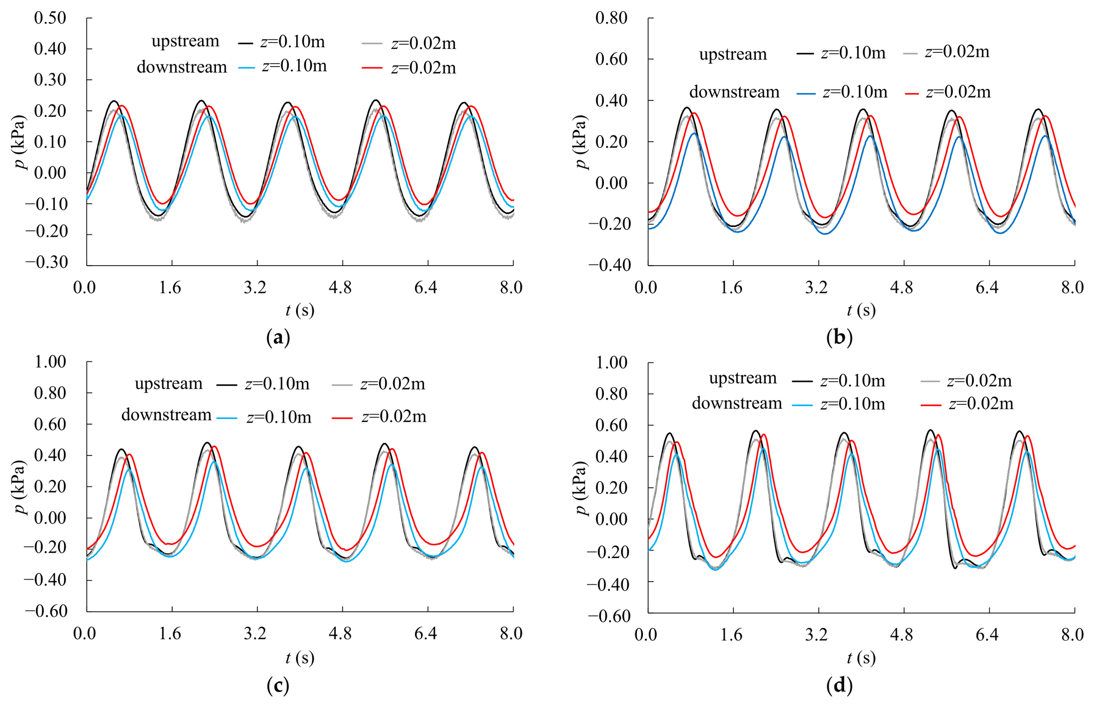
The time histories of pressure at different locations are obtained in each experiment. Figure 12 presents the time histories of pressure under different wave intensities on flat seabed. It is seen that pressure variations at the front and rear sides of the pile follow similar temporal patterns across all heights. Discrepancies are minor and confined to peak magnitudes and their occurrence times. Specifically, the maximum pressure at z = 0.1 m on the wave-facing side is the largest, while at z = 0.02 m, the peak pressure is slightly smaller. Regarding the leeward side, the peak pressures at both positions are smaller than those on the wave-facing side. This is primarily because at the moment of peak pressure, the vortices generated behind the pile column cause pressure reduction. In terms of the occurrence time of peak pressure, due to differences in planar positions, certain phase differences exist between the pressure measurements at the wave-facing and leeward sides.

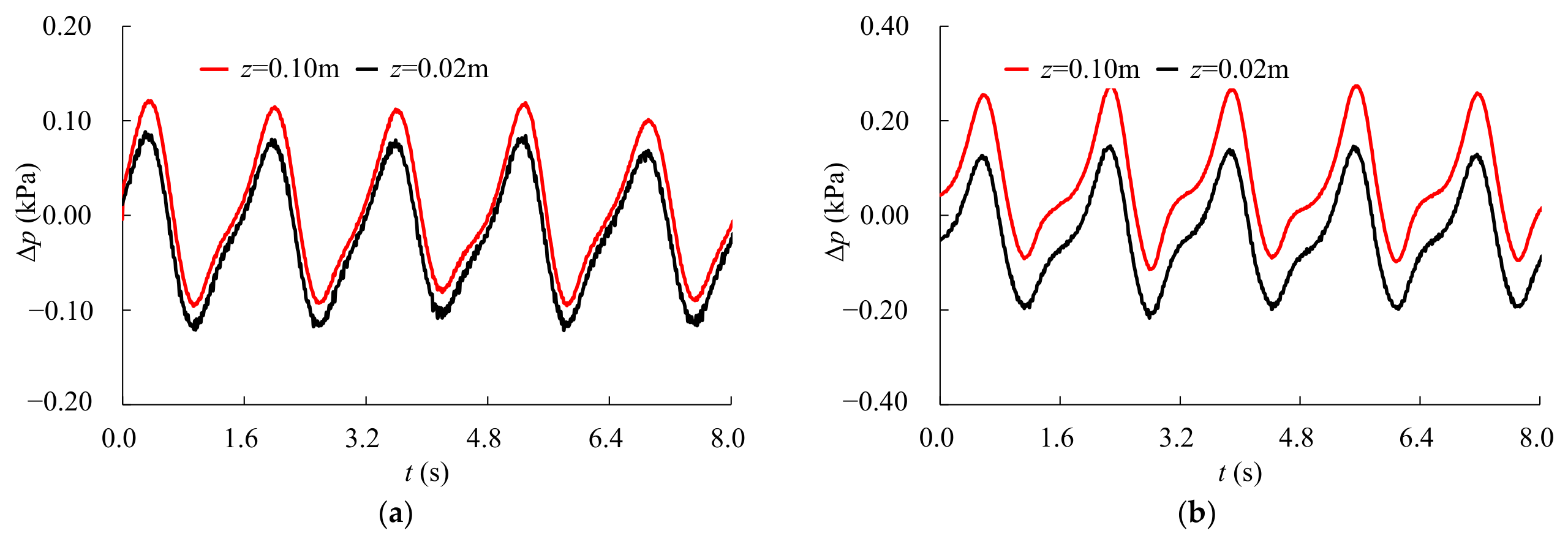
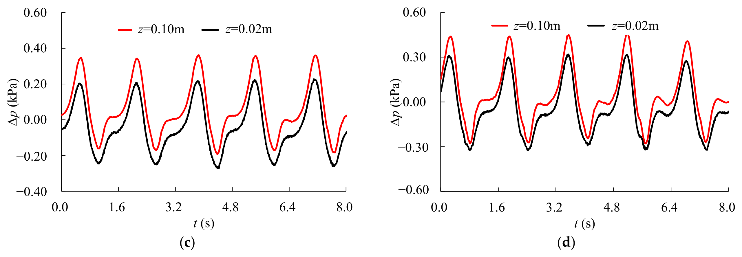
In practical engineering, the differential pressure method is commonly employed to estimate wave–current force. Here, we performed subtraction calculations between the front and rear pressures at the same height on the wave-facing and leeward sides to obtain the pressure differences at various elevations. Figure 13 presents the pressure differences at corresponding heights. The pressure difference Δp similarly exhibits periodic fluctuations following the cyclical variation of waves. In addition, the maximum pressure difference increases monotonically with wave height at both elevations. At z = 0.10 m, it rises from 0.12 kPa (H = 0.04 m) to 0.42 kPa (H = 0.10 m), while at z = 0.02 m, it grows from 0.10 kPa to 0.35 kPa.

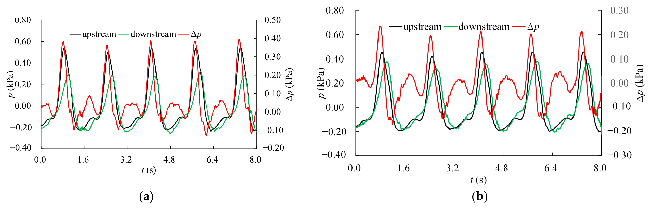
In addition to pure wave conditions, the presence of current in combined wave–current scenarios also affect both the wave–current pressure and pressure difference. Figure 14 presents the pressure and pressure difference variations at different positions with H = 0.08 m and u₀ = 0.33 m/s. It can be observed that under the influence of current, the vortices on the leeward side become relatively intense, resulting in a slightly larger difference between the peak pressures on the wave-facing and leeward sides. Correspondingly, the pressure difference generally remains in a positive pressure state. The higher the elevation, the greater the pressure difference becomes. For instance, at 0.1 m above the bed surface, the maximum pressure difference reaches 0.4 kPa, while at 0.02 m above the bed surface, the pressure difference also attains 0.2 kPa.

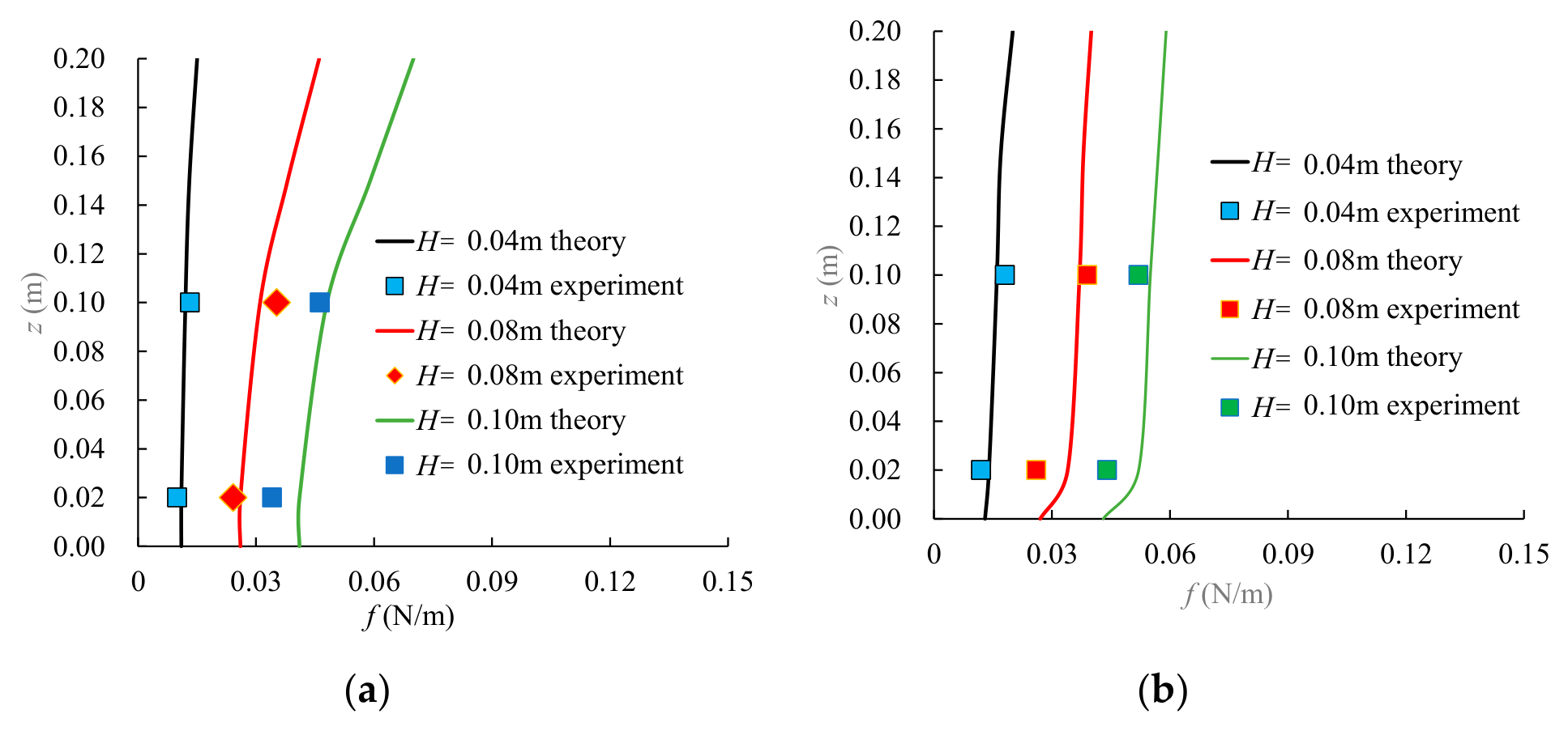
The wave–current force per unit length, denoted as f, at various elevations can be approximately determined by multiplying the pressure difference by the blocking dimension D. Concurrently, under flat bed conditions, the unit length wave–current force can also be theoretically calculated using the Morison equation, as shown in Equation (1). Figure 15 illustrates both the experimental measurements and the theoretical solutions derived from the Morison equation for the unit length wave–current force. It is evident that f increases with elevation, with particularly pronounced vertical variations observed under conditions of large wave heights. In summary, the approach for calculating unit-length wave–current force using the pressure difference between the front and rear surfaces produces results that align closely with theoretical values under conditions of small wave heights. Conversely, under scenarios involving large wave heights, while the vertical distribution of the pressure difference between two points also increases with elevation, the overall calculated values consistently fall short of the theoretical predictions. This suggests that in the context of large wave heights, it is advisable to incorporate additional pressure measurement points to accurately determine the unit length wave–current force.

3.4. Pressure Distribution on Scoured Seabed

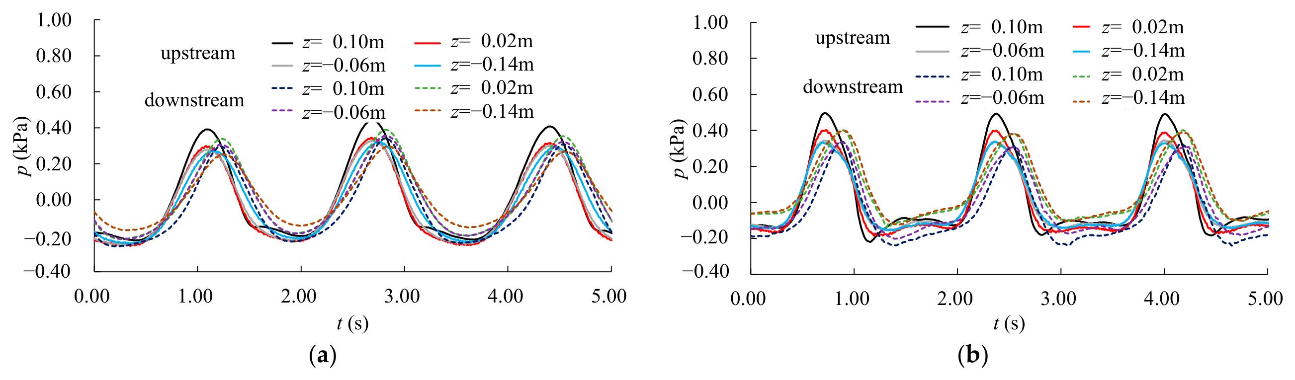
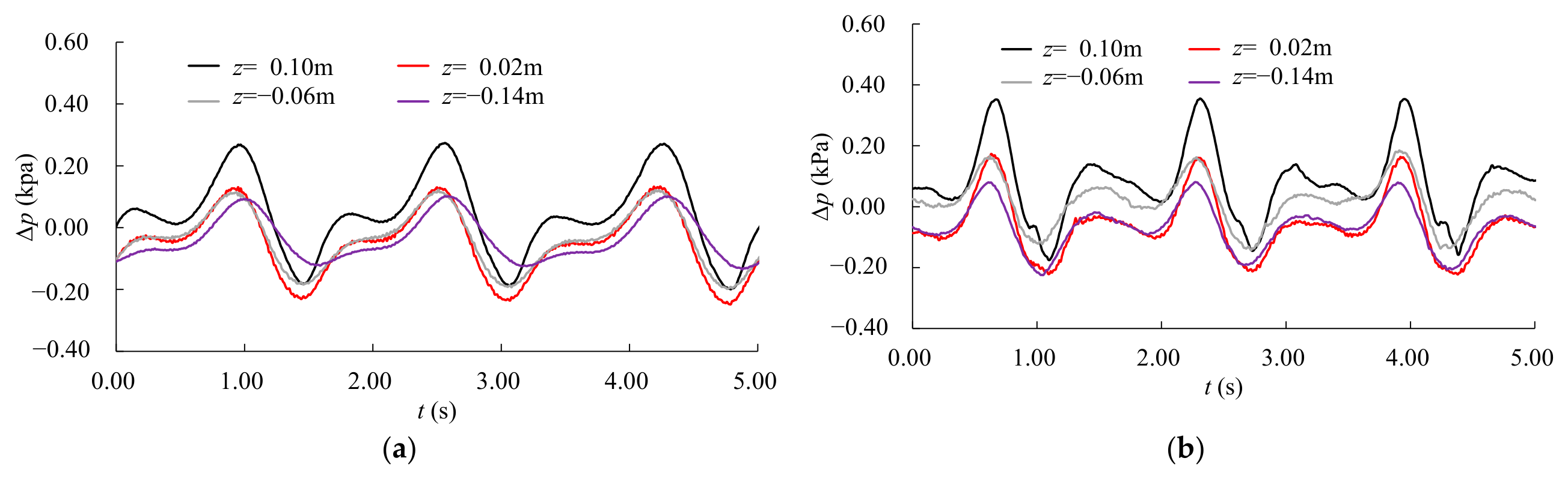
Under scour hole conditions, the pressure values at each point are basically similar to those without a scour hole. The difference lies in that the points within the scour hole also exhibit pressure variations. Figure 16 presents the pressure variations for a wave height of 0.08 m under pure wave conditions and with a current velocity of 0.33 m/s. It can be observed that in the presence of a scour hole, the pressure variation processes at the four points inside the scour hole are relatively similar to those outside the scour hole. Compared to pure wave conditions, the pressure variations under wave–current conditions appear somewhat more irregular, and the maximum pressures are slightly larger than those in the pure wave case. Regarding the pressure difference (Figure 17), these values exhibit periodic variations at different locations, but the maximum pressure differentials vary significantly among different positions.

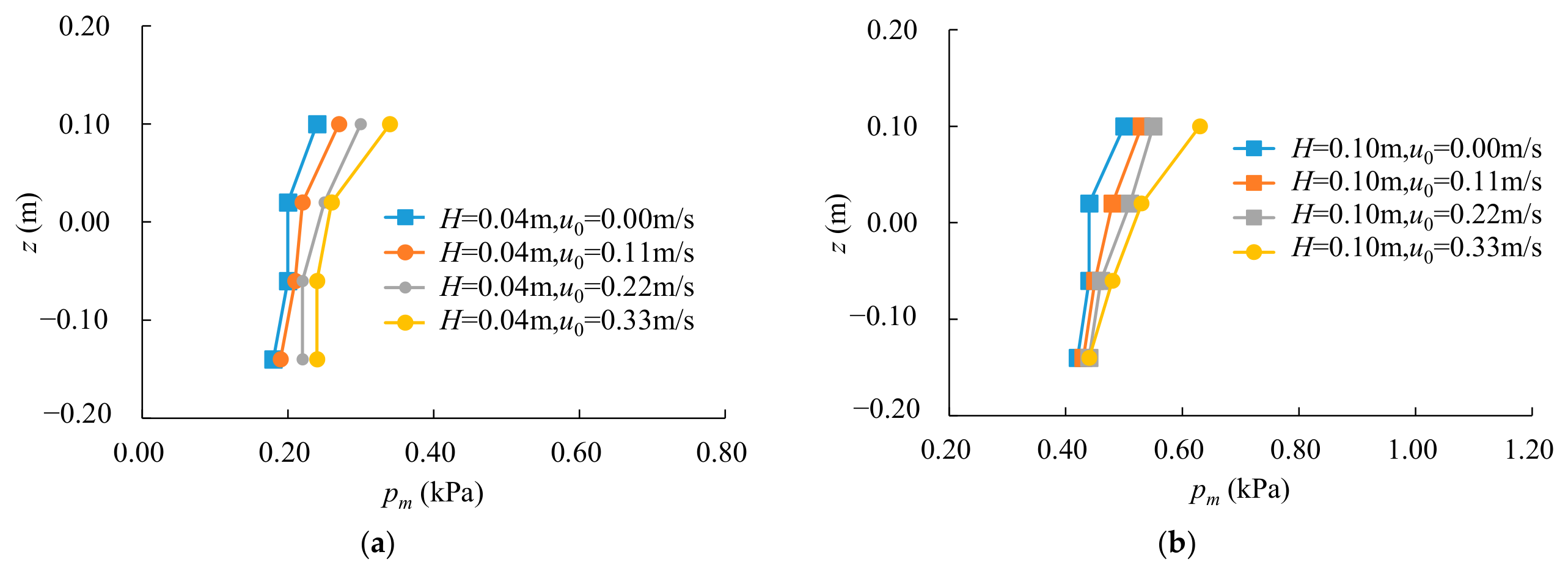
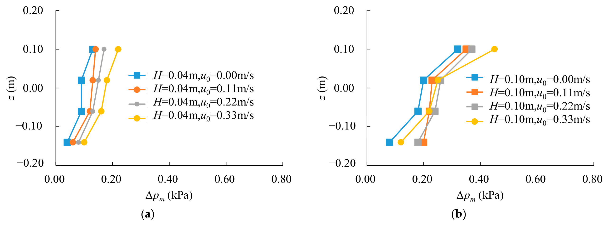
Figure 18 and Figure 19 show the distribution patterns of maximum pressure p_m and the maximum pressure difference ∆p_m at different vertical positions, respectively. In terms of p_m, the closer it is to the seabed, the smaller the maximum pressure value becomes. The difference in p_m between the interior of the scour hole and the region above the bed surface (above 0 m) is within 0.2 kPa. For example, at a wave height of 0.04 m and current velocity of 0.33 m/s, the peak pressure increases from 0.25 kPa to nearly 0.4 kPa, while at a wave height of 0.10 m and current velocity of 0.33 m/s, the maximum pressure increases from 0.4 kPa to 0.6 kPa. Regarding the maximum pressure difference ∆p_m, except for the measurement point located at the bottom of the scour hole where ∆p_m is relatively small (within 0.1 kPa), the ∆p_m at the mid-depth position of the scour hole is basically comparable to that at the position of z = 0.02 m. In summary, when considering the scour hole, the exposed portion of the pile column within the scour hole also generates a net pressure difference, thereby increasing the wave–current loading on the pile column. However, the generally smaller pressure difference values within the scour hole compared to those above the initial seabed indicate that the unit length load acting on the pile column portion inside the scour hole is smaller than that on the pile column above the initial bed surface.

3.5. Effect of Scour on Hydrodynamic Force

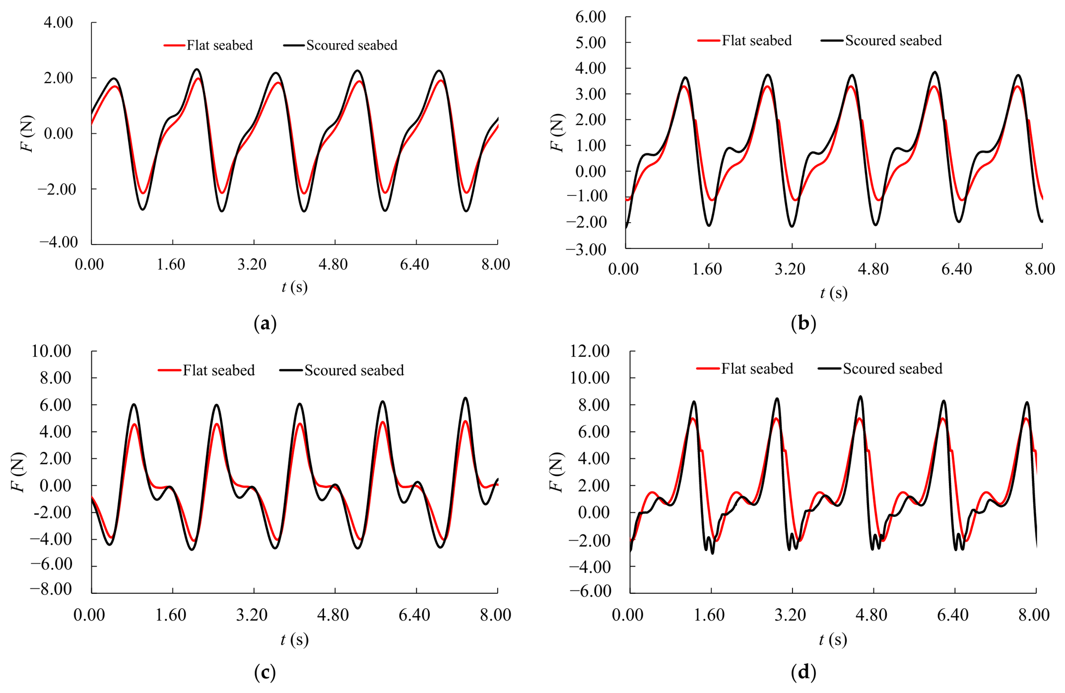
The previous analysis shows that pressure differences in the scour hole create extra forces, but it does not accurately quantify the total wave–current force on the monopile in the experiment. In contrast, numerical simulations can accurately provide a time history of wave–current force. Figure 20 shows simulated wave–current forces for wave heights of 0.04 m and 0.08 m under wave-only and combined wave–current scenarios. For small wave heights, wave force varies linearly. Adding current velocity shifts the force curve positively, creating double-peaked or plateau distortions due to steady drag and nonlinear wave effects. For large wave heights, waves enter the cnoidal regime, where phase differences between drag and inertia force peaks introduce nonlinear features to the wave–current force evolution. In addition, under conditions involving a scour hole, the extended effective length of the pile column exposed to wave–current interactions leads to an increase in both the maximum and minimum wave–current forces.

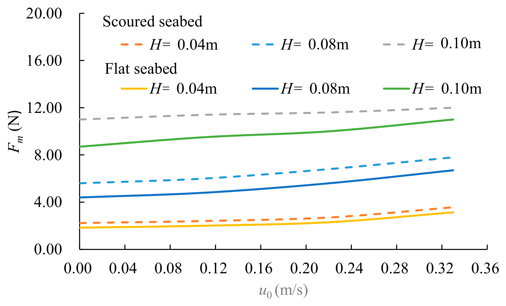
A comprehensive statistical analysis is performed on the maximum wave–current forces F_m under various conditions (Figure 21). The findings reveal that the maximum wave–current force exerted on the pile column exhibits a monotonically increasing pattern with rising approach flow velocity. Concurrently, there is a notable positive correlation between the maximum wave–current force and wave height, with the impact of wave height on loading significantly surpassing that of flow velocity. This observation suggests that in wave–current coupling environments, the inertia force associated with water particle acceleration in waves generally predominates, thereby making wave loading the dominant factor, while the additional contribution from the current velocity remains comparatively minor. Further investigation into the influence of the scour hole indicates that under conditions of seabed scour, the increased effective exposed length of the pile enhances the effective acting area and pressure differential, leading to systematic increases in wave–current forces across all test conditions. It is particularly noteworthy that the absolute increase induced by scour becomes increasingly significant at greater wave heights. Furthermore, the scour-induced amplification of maximum wave–current force amounts to approximately 10–30% relative to that on the flat bed.

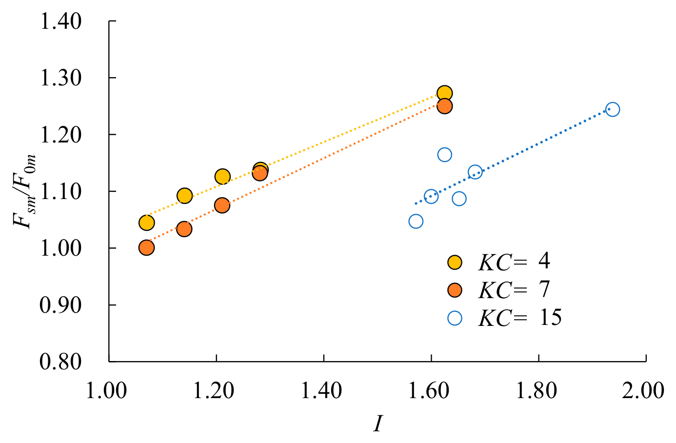
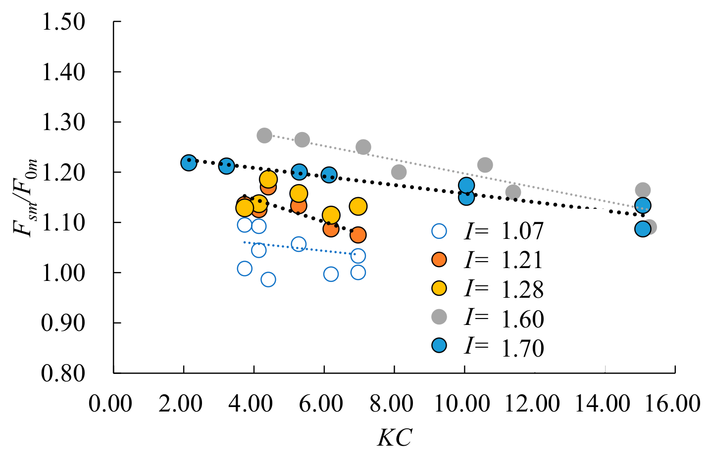
The influence of scour holes on pile loading demonstrates significant dependence on flow regime characteristics. Under steady current (current-dominated) conditions, the total hydrodynamic load on the pile decreases compared to the flat seabed scenario. In contrast, under wave-dominated conditions where pile loading primarily originates from inertia forces induced by water particle acceleration, the formation of a scour hole increases the effective water-structure interaction length on the upstream face of the pile. In this situation, the acceleration effects of the larger water volume become the controlling factor, resulting in a general increasing trend in pile loading. In summary, the key factor influencing the impact of scour holes on pile loading is the balance between inertial and drag forces in wave–current interactions, rather than just the scour depth. This balance is measured by the KC number. A higher KC number means drag forces dominate, while a lower KC number indicates a stronger influence of inertial forces. In addition to KC, a dimensionless post-scour water depth I = (h₀ + d_s + H/2)/(h₀ + H/2) is introduced here to account for the combined effects of scour depth and wave height. Based on present wave–current numerical data and pure wave physical model test data reported by Li et al. [33], the effects of KC and I on monopile maximum wave–current forces are deeply discussed. This study’s research data include KC values ranging from 2 to 15 and I values ranging from 1.07 to 1.94. Using the relative maximum post-scour wave–current force F_sm/F_0m (the ratio of maximum force on scoured seabed to the value on flat seabed) as the evaluation metric, the amplifying effect of scoured topography on structural forces is quantitatively characterized. Figure 22 illustrates how the relative maximum post-scour wave–current force F_sm/F_0m varies with the relative post-scour water depth I. It can be seen that F_sm/F_0m increases with I, indicating that a greater scour depth or larger wave height amplifies the hydrodynamic loading. Quantitatively, over the range of I ≈ 1.0–1.6, the maximum force rises by approximately 23% for KC = 4 (from 1.05 to 1.28) and 25% for KC = 7 (from 1.00 to 1.25). By contrast, for a higher KC of 15, the ratio increases by roughly 19% (from 1.05 to 1.24) over I ≈ 1.5–2.0. At a comparable I value, the amplification is markedly stronger under the lower KC conditions (inertia-dominated regime) than under the drag-dominated condition of KC = 15. Figure 23 further reveals the regulatory role of the KC on the relative maximum post-scour wave–current force. F_sm/F_0m exhibits an overall decreasing trend with increasing KC, and this pattern remains consistent across different I values (ranging from 1.07 to 1.70). This phenomenon can be explained through the composition mechanism of wave forces. At small KC numbers, the inertia force component dominates the total wave–current force. The presence of the scour hole increases both the projected area of water action on the upstream face of the pile and the added mass, leading to significant enhancement of inertial forces. Hence, F_sm/F_0m is markedly greater than 1.0. As the KC number increases, the proportion of the drag force component gradually rises, while the sensitivity of vortex structures to the scour hole geometry decreases relatively, causing the force amplification induced by scour to diminish gradually.

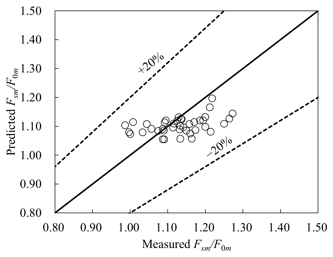
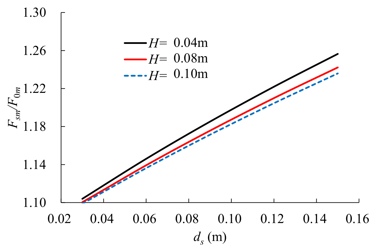
As discussed above, the relative maximum post-scour wave–current force (F_sm/F_0m) is proportional to the relative depth ratio (I) and inversely proportional to the KC. To facilitate practical engineering applications, multivariate regression analysis is employed to derive a predictive equation (Equation (10)) for F_sm/F_0m as a function of I and KC. Figure 24 presents a comparison between the predictions and the research results. Generally, the prediction errors remain within 20%, indicating that the equation is basically reliable. The equation was further employed to investigate the respective contributions of wave height and scour depth within parameter I. Figure 25 indicates that as the scour depth increases from 0.03 m to 0.15 m, the F_sm/F_0m rises markedly from 1.10 to 1.25. By contrast, when the wave height increases from 0.04 m to 0.10 m, the F_sm/F_0m only varies slightly from 1.19 to 1.17. This comparison demonstrates that the F_sm/F_0m is governed primarily by the scour depth rather than the wave height in parameter I.

$${\displaystyle \frac{F_{sm}}{F_{0m}}}=1.20{KC}^{-0.06}{I}^{0.33} 2<KC\le 15$$

(10)

4. Conclusions

This study presents a comprehensive investigation into wave–current force characteristics of monopile foundations under flat bed and scoured bed conditions, utilizing field data, physical experiments, and numerical simulations. The following conclusions are drawn:

(1)

Field scour data analysis implies that prototype-scale scour hole side slopes are considerably gentler than laboratory observations, averaging approximately 1:4 (15°) under bidirectional tidal conditions. Among existing scour depth methods, Zhang’s scour depth equation demonstrates the highest accuracy for field applications, with a relative error of 21% and an RMSE of 1.24 m.

(2)

Under combined wave–current conditions, local scour systematically increases the maximum wave–current force by approximately 10–30% relative to the flat bed value. The relative maximum post-scour force F_sm/F_0m is positively correlated with the dimensionless relative post-scour water depth I (ranging from 1.07 to 1.94) but decreases with increasing KC number (ranging from 2 to 15). A predictive equation is proposed for engineering applications, yielding prediction errors within 20%.

(3)

The present study focuses on KC numbers below 15, where inertia effects remain significant. Future research should extend the KC range to cover higher values fully validate the predictive equation under drag-dominated conditions and further refine its applicability across broader hydrodynamic regimes.

References

1. Sumer, B.M.; Fredsøe, J. The Mechanics of Scour in the Marine Environment; World Scientific: Singapore, 2002. [Google Scholar]
2. Zhang, Z.; Du, S.; He, K.; Guo, Y.; Cheng, W.; Li, Z.; Yang, L.; Zhang, P. Live-bed contraction scour induced by bridge foundations on silty seabed in Hangzhou Bay. Ocean Eng. 2026, 349, 124191. [Google Scholar] [CrossRef]
3. Yu, D.; Wen, M.; Ge, X.; Zhang, Y.; Wan, J.; Lou, S. Semianalytical Solution for One-Dimensional Consolidation of Unsaturated–Saturated Soil Foundations Based on the Interfacial Flow Contact Resistance Model. Int. J. Numer. Anal. Methods Geomech. 2026, 50, 2446–2469. [Google Scholar] [CrossRef]
4. Zhao, Z.; Wang, J.; Shiau, J.; Luo, H.; Yu, D. Probabilistic Analysis of Pile-Reinforced Slopes Considering Anisotropic Spatial Soil Properties. Int. J. Numer. Anal. Methods Geomech. 2026, 50, 1309–1327. [Google Scholar] [CrossRef]
5. Ruan, W.; Qiu, E.; Wu, Z.; Chen, Y.; Sun, B.; Fang, P. Lazy wave configuration for shallow-water dynamic power cables of floating wind turbines: RUC-derived stiffness characterization and global response analysis. Ocean Eng. 2026, 352, 124640. [Google Scholar] [CrossRef]
6. Melville, B.; Chiew, Y. Time Scale for Local Scour at Bridge Piers. J. Hydraul. Eng. 1999, 125, 59–65. [Google Scholar] [CrossRef]
7. Chiew, Y.M.; Melville, B.W. Local scour around bridge piers. J. Hydraul. Res. 1987, 25, 15–26. [Google Scholar] [CrossRef]
8. Yuan, C.; Melville, B.W.; Adams, K.N. Scour at wind turbine tripod foundation under steady flow. Ocean Eng. 2017, 141, 277–282. [Google Scholar] [CrossRef]
9. Richardson, E.V.; Davis, S.R. Evaluating Scour at Bridge, 4th ed.; Hydraulic Engineering Circular No. 18 (HEC-18); Federal Highway Administration, U.S. Department of Transportation: Washington, DC, USA, 2001.
10. Coleman, S.E.; Lauchlan, C.S.; Melville, B.W. Clear-water scour development at bridge abutments. J. Hydraul. Res. 2003, 41, 521–531. [Google Scholar] [CrossRef]
11. Ettmer, B.; Orth, F.; Link, O. Live-Bed Scour at Bridge Piers in a Lightweight Polystyrene Bed. J. Hydraul. Eng. 2015, 141, 4015017. [Google Scholar] [CrossRef]
12. Ting, F.C.K.; Briaud, J.L.; Chen, H.C.; Gudavalli, R.; Perugu, S.; Wei, G.S. Flume Tests For Scour in Clay at Circular Piers. J. Hydraul. Eng. 2001, 127, 969–978. [Google Scholar] [CrossRef]
13. Sumer, B.; Fredsøe, J. Wave Scour around a Large Vertical Circular Cylinder. J. Waterw. Port Coast. Ocean Eng. 2001, 127, 125–134. [Google Scholar] [CrossRef]
14. Sumer, B.; Fredsøe, J. Scour around Pile in Combined Waves and Current. J. Hydraul. Eng. 2001, 127, 403–411. [Google Scholar] [CrossRef]
15. Qi, W.; Gao, F. Equilibrium scour depth at offshore monopile foundation in combined waves and current. Sci. China Technol. Sci. 2014, 57, 1030–1039. [Google Scholar] [CrossRef]
16. Guan, D.; Xie, Y.; Chiew, Y.; Ding, F.; Ferradosa, T.F.; Hong, J. Estimation of local scour around monopile foundations for offshore structures using machine learning models. Ocean Eng. 2024, 296, 116951. [Google Scholar] [CrossRef]
17. Zhang, Z.; Guo, Y.; Yang, Y.; Shi, B.; Wu, X. Scale Model Experiment on Local Scour around Submarine Pipelines under Bidirectional Tidal Currents. J. Mar. Sci. Eng. 2021, 9, 1421. [Google Scholar] [CrossRef]
18. Han, H.; Chen, Y.; Sun, Z. Estimation of Maximum Local Scour Depths at Multiple Piles of Sea/Bay-crossing Bridges. KSCE J. Civ. Eng. 2019, 23, 567–575. [Google Scholar] [CrossRef]
19. Schendel, A.; Hildebrandt, A.; Goseberg, N.; Schlurmann, T. Processes and evolution of scour around a monopile induced by tidal currents. Coast. Eng. 2018, 139, 65–84. [Google Scholar] [CrossRef]
20. Zhang, Z.; Du, S.; Guo, Y.; Yang, Y.; Zeng, J.; Sui, T.; Wei, R.; Li, Z. Field study of local scour around bridge foundations on silty seabed under irregular tidal flow. Coast. Eng. 2023, 185, 104382. [Google Scholar] [CrossRef]
21. Wang, S.; Qi, W.; Li, B.; Wang, C.; Gao, F. Tidal currents-induced scour development around pile foundations: Effects of flow velocity hydrograph. Coast. Eng. 2024, 191, 104533. [Google Scholar] [CrossRef]
22. Zhang, N.; Qiu, G.; Zhao, W.; Zhai, W.; Yin, S.; Zheng, Y. Scour around offshore wind turbine monopile foundations under tidal flow: CFD-DEM coupled approach. Ocean Eng. 2026, 343, 123411. [Google Scholar] [CrossRef]
23. Høgedal, M.; Hald, T. Scour assessment and design for monopile foundations for offshore wind turbines. In Proceedings of the Copenhagen Offshore Wind, Copenhagen, Denmark, 26–28 October 2005. [Google Scholar]
24. Harris, J.M.; Whitehouse, R.J.S.; Sutherland, J. Marine Scour and Offshore Wind: Lessons Learnt and Future Challenges. In Proceedings of the 30th International Conference on Ocean, Offshore and Arctic Engineering, Rotterdam, The Netherlands, 19–24 June 2011. [Google Scholar]
25. Whitehouse, R.J.S.; Harris, J.M.; Sutherland, J.; Rees, J. The nature of scour development and scour protection at offshore windfarm foundations. Mar. Pollut. Bull. 2011, 62, 73–88. [Google Scholar] [CrossRef]
26. Dixen, F.H.; Dixen, M.; Pedersen, J.; Dahl, J.F. Scour Development Around Offshore Wind Turbine Foundation: Field Measurement & Analysis. In Proceedings of the 6th International Conference on Scour and Erosion, Paris, France, 27–31 August 2012. [Google Scholar]
27. Morison, J.R.; Johnson, J.W.; Schaaf, S.A. The Force Exerted by Surface Waves on Piles. J. Pet. Technol. 1950, 2, 149–154. [Google Scholar] [CrossRef]
28. Sumer, B.M.; Fredsøe, J. Hydrodynamics Around Cylindrical Structures; World Scientific: Singapore, 2006. [Google Scholar]
29. Wolfram, J.; Naghipour, M. On the estimation of Morison force coefficients and their predictive accuracy for very rough circular cylinders. Appl. Ocean Res. 1999, 21, 311–328. [Google Scholar] [CrossRef]
30. Yuan, Z.; Huang, Z. An experimental study of inertia and drag coefficients for a truncated circular cylinder in regular waves. J. Hydrodyn. 2010, 22, 318–323. [Google Scholar] [CrossRef]
31. Li, Y.; Wang, F.; Kang, H. Wave-Current Forces on Slender Circular Cylinders. China Ocean Eng. 1991, 5, 287–310. [Google Scholar]
32. Sui, T.; Liu, C.; Zhang, J.; Zhang, C.; Zheng, J. 3D numerical modeling of wave–monopile–seabed interaction in the presence of a scour hole. Ocean Eng. 2024, 298, 117254. [Google Scholar] [CrossRef]
33. Li, B.; Qi, W.; Gao, F.; He, B.; Yang, L. Experimental investigation of scour effects on regular and breaking wave loads on a monopile. Coast. Eng. 2025, 197, 104696. [Google Scholar] [CrossRef]
34. Aksel, M.; Yagci, O.; Kirca, V.S.O.; Erdog, E.; Heidari, N. A comparative analysis of coherent structures around a pile over rigid-bed and scoured-bottom. Ocean Eng. 2021, 226, 108759. [Google Scholar] [CrossRef]
35. Wang, Z.; Huan, C.; Chen, L. Research of Real-time Monitoring for Local Scour of Offshore Wind Power Pile Foundation Based on Sonar Image. J. Ocean Technol. 2023, 42, 91–99. [Google Scholar]
36. Whitehouse, R.J.S.; Stroescu, E.I. Scour depth development at piles of different height under the action of cyclic (tidal) flow. Coast. Eng. 2023, 179, 104225. [Google Scholar] [CrossRef]
37. Zhao, E.; Mu, L.; Qin, H.; Jiang, H. Study on dynamic slope angle of sandy seabed around the submarine piggyback pipeline in steady flow. J. Mar. Eng. Technol. 2021, 20, 324–336. [Google Scholar] [CrossRef]
Figure 1. Typical scour profile around OWF.
Jmse 14 00989 g001
Figure 2. Wave–current flume experiment: layout and photo. (a) Vertical layout of the experiment setup; (b) experimental photo.
Jmse 14 00989 g002
Figure 3. Repeatability tests of wave–current pressure (a) H = 0.04 m, u0 = 0.33 m/s; (b) H = 0.10 m, u0 = 0.33 m/s.
Jmse 14 00989 g003
Figure 4. Computational domain and mesh distribution. (a) Computational domain; (b) mesh distribution around a monopile.
Jmse 14 00989 g004
Figure 5. Grids sensitivity.
Jmse 14 00989 g005
Figure 6. Validation of time process of upstream pressure: H = 0.04 m, u0 = 0.33 m/s, scoured seabed. (a) Gauge No. 1; (b) Gauge No. 2; (c) Gauge No. 3; (d) Gauge No. 4.
Jmse 14 00989 g006
Figure 7. Validation of time process of upstream pressure: H = 0.08 m, u0 = 0.33 m/s, scoured seabed. (a) Gauge No. 1; (b) Gauge No. 2; (c) Gauge No. 3; (d) Gauge No. 4.
Jmse 14 00989 g007
Figure 8. Validation of time process of upstream pressure: H = 0.04 m, u0 = 0.33 m/s, flat seabed. (a) Gauge No. 1; (b) Gauge No. 2.
Jmse 14 00989 g008
Figure 9. Validation of time process of upstream pressure: H = 0.08 m, u0 = 0.33 m/s, flat seabed. (a) Gauge No. 1; (b) Gauge No. 2.
Jmse 14 00989 g009
Figure 10. Comparison of different predicted methods versus field data.
Jmse 14 00989 g010
Figure 11. Scour hole profile in different directions [23,24,35,36]. (a) Inflow direction; (b) crossflow direction.
Jmse 14 00989 g011
Figure 12. Time history of pressure at various points. (a) H = 0.04 m, u0 = 0.0 m/s; (b) H = 0.06 m, u0 = 0.0 m/s; (c) H = 0.08 m, u0 = 0.0 m/s; (d) H = 0.10 m, u0 = 0.0 m/s.
Jmse 14 00989 g012
Figure 13. Time history of pressure differences at different elevations. (a) H = 0.04 m, u0 = 0.0 m/s; (b) H = 0.06 m, u0 = 0.0 m/s; (c) H = 0.08 m, u0 = 0.0 m/s; (d) H = 0.10 m, u0 = 0.0 m/s.
Jmse 14 00989 g013aJmse 14 00989 g013b
Figure 14. Time histories of pressure and pressure difference (H = 0.08 m, u0 = 0.33 m/s). (a) z = 0.1 m; (b) z = 0.02 m.
Jmse 14 00989 g014
Figure 15. Vertical distribution of wave–current force per unit length. (a) u0 = 0.00 m/s; (b) u0 = 0.33 m/s.
Jmse 14 00989 g015
Figure 16. Time histories of pressure at different points. (a) H = 0.08 m, u0 = 0.0 m/s; (b) H = 0.08 m, u0 = 0.33 m/s.
Jmse 14 00989 g016
Figure 17. Time histories of the pressure difference. (a) H = 0.08 m, u0 = 0.0 m/s; (b) H = 0.08 m, u0 = 0.33 m/s.
Jmse 14 00989 g017
Figure 18. Vertical distribution of the maximum pressure at the upstream side. (a) H = 0.04 m; (b) H = 0.10 m.
Jmse 14 00989 g018
Figure 19. Vertical distribution of the maximum pressure difference. (a) H = 0.04 m; (b) H = 0.10 m.
Jmse 14 00989 g019
Figure 20. Time series of wave–current forces in different cases. (a) H = 0.04 m, u0 = 0.00 m/s; (b) H = 0.04 m, u0 = 0.33 m/s; (c) H = 0.08 m, u0 = 0.00 m/s; (d) H = 0.08 m, u0 = 0.33 m/s.
Jmse 14 00989 g020
Figure 21. Maximum wave–current forces in different cases.
Jmse 14 00989 g021
Figure 22. Variation in the relative maximum post-scour force with relative post-scour water depth.
Jmse 14 00989 g022
Figure 23. Variation in the relative maximum post-scour force with KC.
Jmse 14 00989 g023
Figure 24. Comparisons of measured and predicted Fsm/F0m values.
Jmse 14 00989 g024
Figure 25. Variation in the relative maximum post-scour force with absolute scour depth.
Jmse 14 00989 g025