Article

Optimization of Extreme Design Parameters for Swell-Dominated Waves Using a Gaussian Mixture Model

1
Shandong Electric Power Engineering Consulting Institute Co., Ltd., Jinan 250013, China
2
College of Engineering, Ocean University of China, Qingdao 266100, China
*
Author to whom correspondence should be addressed.
J. Mar. Sci. Eng. 2026, 14(11), 988; https://doi.org/10.3390/jmse14110988
Submission received: 18 April 2026 / Revised: 22 May 2026 / Accepted: 22 May 2026 / Published: 27 May 2026
(This article belongs to the Special Issue Breakthrough Research in Marine Structures)

Abstract

Environmental condition assessment is essential for the design of floating wind turbines, particularly when determining design sea states that balance safety and economy. The environmental contour method, typically constructed through the Inverse First Order Reliability Method combined with parametric joint distributions, is widely adopted for this purpose. However, conventional models often struggle to adequately characterize complex sea states involving mixed wind and swell systems, which exhibit multimodality and irregular dependence structures. To address this limitation, this study applies the use of Gaussian mixture models (GMM) to construct environmental contours. The GMM-based approach models the joint distribution of environmental variables in a flexible and data-adaptive manner, with the number of mixture components determined by the Bayesian Information Criterion and model parameters estimated via the expectation-maximization algorithm. Compared with the conventional conditional Weibull–Lognormal model, the GMM significantly improves fitting accuracy: the RMSE decreases from approximately 0.06 to below 0.0013, and the R2 increases to nearly 1.000 across all three datasets. The KS and χ2 tests confirm that the GMM adequately fits the observed data at the 0.05 significance level, whereas the baseline model is rejected in several cases. For the 100-year return period, the GMM yields maximum significant wave heights of 4.19–4.55 m with associated peak periods of 18.8–20.3 s, while the baseline model gives 4.02–4.18 m and 14.3–14.6 s, respectively. These quantitative improvements demonstrate that the mixture-based contours capture the intricate characteristics of wind–swell coexisting sea conditions more accurately, leading to enhanced representativeness of extreme sea states. Consequently, the adopted method enables more refined and reliable design sea state assessments for tested datasets, contributing to the optimization of environmental parameter selection for floating wind turbines.

1. Introduction

Marine structures operating in offshore environments are constantly subjected to challenging sea conditions that directly influence their design, operational safety, and lifecycle integrity. Within the framework of reliability-based design, the accurate characterization of extreme environmental conditions is paramount for ensuring structural adequacy while maintaining economic viability. The environmental contour (EC) method has emerged as a widely adopted approach for identifying critical sea states and estimating long-term extreme responses of marine structures [1,2,3]. This method offers a practical compromise between computational efficiency and analytical rigor by decoupling the environmental description from the structural response analysis. Typically, ECs are constructed using the Inverse First Order Reliability Method (IFORM) in conjunction with joint probability models that capture the dependencies among metocean variables such as significant wave height, wave period, wind speed, and current velocities [4,5,6].
The accuracy and reliability of environmental contours are fundamentally contingent upon the fidelity of the underlying joint probability model [7,8]. Over the past decades, various statistical approaches have been developed to characterize the joint distribution of environmental parameters (Table 1). Early efforts relied on parametric bivariate distribution functions, such as the bivariate Lognormal model proposed by Ochi [9] for wave height and period. However, these simple parametric forms often prove insufficient for capturing the intricate dependence structures inherent in real-world oceanographic data. The conditional modeling approach has gained considerable popularity, wherein the joint distribution is constructed through a marginal distribution combined with conditional probability functions [10,11,12,13,14]. Notable examples include the Burr-Lognormal conditional model applied by Clarindo and Guedes Soares [15] for wave data, as well as the Weibull–Lognormal framework extensively employed in engineering practice. While these conditional models offer computational tractability, they impose predefined functional forms that may inadequately represent nonlinear dependencies or asymmetric tail behaviors, features that are critically important for extreme value estimation.
Copula-based models have emerged as a flexible alternative, enabling separate specification of marginal distributions and dependence structures [16,17,18]. By decoupling these two components, copulas allow for greater flexibility in capturing complex dependence patterns, including upper and lower tail dependencies that are particularly relevant for extreme sea state characterization. Studies by Montes-Iturrizaga and Heredia-Zavoni [19,20] have demonstrated the application of bivariate and vine copulas for environmental contour construction. Nonetheless, parametric copulas still impose assumptions regarding the functional form of dependence, which may be restrictive when dealing with heterogeneous datasets that exhibit multimodal characteristics or varying dependence regimes across the data domain [21,22].
Nonparametric methods, such as kernel density estimation (KDE), offer an alternative that avoids prespecified parametric forms [23,24]. These approaches can adapt to the empirical data distribution without imposing strong assumptions, yet they face challenges related to bandwidth selection and may produce contours that are overly sensitive to sampling variability. Furthermore, nonparametric methods often require substantial data volumes to achieve stable estimates, particularly in the tail regions where extreme environmental conditions reside. The serial correlation present in environmental time series further complicates the estimation of extreme events and environmental contours [25,26].
A notable limitation of conventional approaches, whether parametric, conditional, or copula-based, lies in their struggle to adequately characterize complex sea states involving mixed wind and swell systems. Such conditions frequently exhibit multimodality, irregular dependence structures, and distinct subpopulations that cannot be captured by single-distribution models. This challenge is particularly acute in regions where distinct wave systems coexist, such as the Indonesian archipelago, where the interplay between local wind seas and distant swell systems creates heterogeneous wave climates. The presence of multiple wave regimes necessitates modeling frameworks capable of representing multimodal distributions while maintaining consistency between marginal and joint characteristics [27,28]. To address these limitations, mixture distribution models have gained increasing attention in ocean engineering applications. The Gaussian mixture model (GMM) offers a flexible and versatile framework that combines the mathematical tractability of Gaussian components with the capacity to approximate arbitrary probability distributions through linear combinations of component densities [29]. By adjusting the number of mixture components, GMM can adapt to data with varying degrees of complexity, from unimodal to multimodal structures. The Expectation-Maximization (EM) algorithm provides an efficient means for parameter estimation, while information criteria such as the Bayesian Information Criterion (BIC) enable objective selection of the optimal number of components. These properties make GMM particularly well-suited for modeling metocean data that exhibit complex, multimodal characteristics arising from mixed sea conditions.
Table 1. Comparison of different joint distribution approaches for environmental contour construction.
Method CategoryRepresentative StudiesKey CharacteristicsLimitations
Conventional conditional modelsOchi [9]; Agarwal and Manuel [10]; Vanem et al. [11]; Kwon et al. [12]; Beshbichi et al. [13]; Zhao and Dong [14]; Clarindo and Guedes Soares [15]Marginal Weibull + conditional Lognormal with polynomial functions; computationally efficientPoor tail fitting; fails for multimodal data; parametric dependence assumptions
Copula-based methodsFang et al. [16]; Zhao and Dong [17]; Li and Wei [18]; Montes-Iturrizaga and Heredia-Zavoni [19,20]; Heredia-Zavoni and Montes-Iturrizaga [21]; Wu et al. [22]Separate marginal and dependence modeling; flexible tail dependencePrespecified copula families; limited for high dimensions; still parametric
KDE/NonparametricWang [23]; Jiang et al. [24]Data-adaptive; no parametric assumptionsSensitive to bandwidth; large data required; unstable tails
Existing mixed model methodsLucas and Guedes Soares [27]; Li et al. [28]; Zhao et al. [29]Multimodal capability; EM + BIC; IFORM contoursEvaluated on open-ocean sites; limited comparison with standard conditional model
This study (GMM-IFORM)Zhao et al. [29]Application to mixed wind-swell seas vs. general open-ocean; Indonesian hindcast vs. NDBC buoys; strong bimodality vs. weak multimodality; tail-specific metrics, hold-out, cross-validation vs. basic fitting; explicit extraction of design sea states for floating wind turbines vs. not providedRef. [29] used open-ocean datasets with weaker multimodality, no methodological innovation over Ref. [29]
This study aims to enhance the accuracy and reliability of environmental contour-based design sea state assessment for floating wind turbines by employing GMMs within the IFORM framework. The adopted approach offers several key advantages over conventional methods: (1) the flexibility to capture multimodal joint distributions arising from mixed wind and swell systems; (2) the capacity to model both marginal and joint characteristics within a unified framework; and (3) data-adaptive model selection through information criteria that balance goodness-of-fit with model complexity. It is important to note that this study does not propose a new contour algorithm; rather, it extends the applicability of the existing GMM-IFORM to mixed wind-swell dominated sea states and provides a comprehensive validation framework including tail-specific error metrics, out-of-sample testing, bootstrap uncertainty bands, and design sea state extraction. Section 2 introduces the theoretical foundations underlying the environmental contour approach, covering the IFORM methodology and the conventional conditional joint distribution model commonly used in practice. Section 3 presents the GMM, detailing its formulation, the EM algorithm for parameter estimation, and the BIC for model selection. Section 4 provides an overview of the environmental data employed in this study, with emphasis on the mixed wind and swell conditions characteristic of Indonesian waters, followed by the implementation of the contour construction procedure and a comparative evaluation between the adopted mixture-based method and the conventional conditional Weibull–Lognormal model. Section 5 discusses the results, highlighting the improvements achieved through the mixture-based approach and its implications for design sea state assessment.

2. Theoretical Background

This section presents the theoretical foundations underlying environmental contour construction. The conventional IFORM-based contour method is first introduced, followed by a description of the commonly used conditional joint distribution model for wave variables. The limitations of conventional approaches are then discussed, motivating the adoption of mixture models for improved representation of complex sea states.

2.1. IFORM-Based Environmental Contours

In the reliability-based design of floating wind turbines, the long-term extreme response associated with a specified return period serves as a critical input for assessing structural integrity. For a target return period of N years, the extreme response sN can be expressed as
s N = F S 1 ( 1 P f )
where F S 1 ( ) denotes the inverse cumulative distribution function of the long-term extreme response, and Pf represents the failure probability corresponding to the N-year return period.
Considering the environmental variability, the failure probability can be formulated through the integration of the short-term response over the joint distribution of environmental variables. Let X = ( X 1 , X 2 , , X n ) T denote the vector of metocean variables (e.g., significant wave height Hs, wave peak period Tp, wind speed Vs), and let g(X) represent the limit state function that defines the boundary between safe and failure domains. The failure probability is then given by
P f = g ( X ) 0 f X ( x ) d x
where fX(x) is the joint probability density function of the environmental variables.
In the FORM, the failure boundary is approximated by a first-order Taylor expansion at the design point, the point on the limit state surface with the highest probability density. The reliability index β is defined as the minimum distance from the origin to the limit state surface in the standard Gaussian space. The Inverse FORM employs this concept to construct environmental contours by tracing the set of points that correspond to a constant reliability index in the physical space, thereby decoupling the environmental description from the structural response analysis. The design failure probability Pf is expressed as
P f = 1 N λ
where N is the return period in years, and λ = 8760 is the number of independent hourly sea states per year (sea-state duration = 1 h). The failure probability Pf is thus the exceedance probability per individual sea state.
The transformation from the physical space to the standard Gaussian space is achieved through the Rosenblatt transformation. For bivariate wave data consisting of significant wave height Hs and spectral peak period Tp, points on the contour in the standard Gaussian space lie on a circle of radius βF,
u 1 = β F sin θ ,   u 2 = β F cos θ , θ 0 , 2 π
where U = (u1, u2) are independent standard normal variables. The corresponding environmental variables in the physical space are obtained via the inverse Rosenblatt transformation:
x 1 = F X 1 1 [ Φ ( u 1 ) ] ,   x 2 = F X 2 | X 1 1 [ Φ ( u 1 ) | x 1 ]
where Φ ( ) denotes the cumulative distribution function of the standard normal distribution, and F X 1 1 ( ) and F X 2 | X 1 1 ( ) represent the inverse marginal and conditional cumulative distribution functions, respectively.

2.2. Conditional Joint Distribution Model

Among various approaches for modeling the joint distribution of wave parameters, the conditional modeling framework has gained widespread acceptance and is recommended by several design standards (e.g., DNV [30]). In this framework, the joint probability density function of Hs and Tp is expressed as the product of the marginal distribution of Hs and the conditional distribution of Tp given Hs:
f H s , T p ( h s , t p ) = f H s ( h s ) f T p | H s ( t p | h s )
For the marginal distribution of significant wave height, the three-parameter Weibull distribution is commonly employed due to its flexibility in capturing the tail behavior:
F H s ( h s ) = 1 exp h s γ α β , h s γ
where α > 0 is the scale parameter, β > 0 is the shape parameter, and γ is the location parameter. These parameters are typically estimated using the maximum likelihood method.
The conditional distribution of wave period given wave height is frequently modeled using a lognormal distribution:
f T p | H s ( t p | h s ) = 1 t p 2 π σ ( h s ) e x p ln t p μ ( h s ) 2 2 σ 2 ( h s )
where the conditional mean μ(hs) and conditional standard deviation σ(hs) are expressed as functions of Hs. In practice, these functions are often approximated by polynomial forms, such as quadratic or cubic polynomials, fitted to the data using nonlinear least squares regression:
μ ( h s ) = a 0 + a 1 h s + a 2 h s 2 , σ ( h s ) = b 0 + b 1 h s + b 2 h s 2
Higher-order polynomial terms may be introduced when necessary to capture more complex dependencies. The coefficients are estimated from the available measurements by minimizing the sum of squared residuals.

2.3. Limitations of Conventional Models and Motivation for Improvement

Despite the widespread application of the conditional joint distribution approach, its performance in constructing accurate environmental contours can be inconsistent across different geographical locations and sea state characteristics. Several limitations inherent to conventional models motivate the exploration of more flexible alternatives. First, the marginal distribution of significant wave height is typically represented by a single parametric distribution, such as the three-parameter Weibull model. While such models often provide acceptable fits for the bulk of the data, they may exhibit considerable discrepancies in the upper tail region, which is of primary importance for extreme value estimation. Overestimation or underestimation of extreme wave heights can lead to non-conservative or overly conservative structural designs. Various alternative distributions have been explored in the literature to improve tail fitting, including the exponentiated Weibull distribution [31], the Burr distribution [15], and hybrid models combining lognormal and Weibull components [32]. Nevertheless, no single parametric form has been found to universally outperform others across all sea areas, underscoring the need for data-adaptive approaches. Second, the conditional distribution parameters of wave period are often approximated using low-order polynomial functions of wave height. This parametric assumption may inadequately capture the true dependence structure, particularly when the relationship between Hs and Tp exhibits nonlinearity, heteroscedasticity, or multimodality. In cases where the wave climate comprises multiple generating mechanisms, such as the coexistence of local wind seas and distant swells, the conditional relationship can become highly complex and may not be well represented by any smooth function of Hs alone. This limitation not only affects the accuracy of the joint distribution but also propagates to the resulting environmental contours, potentially biasing the estimated extreme sea states. Third, the challenge of accurately modeling multivariate environmental data extends beyond the conditional framework. Alternative approaches, including multivariate parametric distributions and copula-based models, also face limitations when confronted with complex dependence structures. Parametric copulas impose predefined forms of dependence that may not align with the actual data characteristics, while nonparametric methods, though flexible, are susceptible to sampling variability and require large datasets for reliable estimation in the tail regions. Furthermore, none of these conventional approaches are designed to handle multimodal distributions that naturally arise in mixed sea conditions, where distinct wave populations coexist and contribute to the overall environmental variability.
The complexity of real-world ocean environments, particularly in regions such as Indonesian waters, where wind seas and swells frequently interact, necessitates modeling frameworks capable of capturing multimodal characteristics and intricate dependence structures without imposing restrictive parametric assumptions. Mixture models offer a promising solution by combining multiple component distributions to approximate arbitrarily complex probability densities. Among these, the GMM provides a mathematically tractable and computationally efficient framework that can adapt to the underlying data structure through the selection of an appropriate number of components. By enabling the joint distribution to be represented as a weighted sum of Gaussian components, GMM can effectively capture the multimodal nature of mixed sea states while maintaining the ability to model both marginal and joint characteristics consistently.
This study therefore adopts the GMM within the IFORM framework to construct environmental contours for floating structure design. The flexibility of GMM, combined with systematic parameter estimation via the expectation-maximization algorithm and component selection using the Bayesian information criterion, offers a robust alternative to conventional approaches. The following sections detail the formulation and implementation of this mixture-based method, with application to wave data from Indonesian waters characterized by complex wind–swell interactions.

3. Gaussian Mixture Model for Environmental Variables

The GMM provides a flexible parametric framework for characterizing environmental data exhibiting complex, multimodal structures. This approach assumes that the overall data distribution can be represented as a weighted combination of multiple Gaussian components, each capturing a distinct underlying subpopulation. In this section, the formulation of the finite GMM is presented, followed by a description of the EM algorithm for parameter estimation. The criteria used for model selection and goodness-of-fit assessment are also introduced.

3.1. Mixture Model Formulation and EM Algorithm

For a set of d-dimensional environmental observations X = {x1, x2, …, xn}, the finite mixture model can be expressed as [33]
f ( x ; ξ ) = k = 1 K π k f k ( x ; θ k )
where K denotes the number of mixture components, πk represents the mixing weight for the kth component satisfying k = 1 K π k = 1 and 0 < π k 1 , and fk(x; θk) is the probability density function of the kth component with parameter vector θk. The complete set of unknown parameters is denoted as ξ = ( π 1 , , π K , θ 1 , , θ K ) . Both the number of components K and the parameters ξ must be determined from the data.
When adopting a multivariate GMM to describe the joint distribution of environmental variables, each component follows a Gaussian distribution. The overall probability density function is then given by
f ( x ; ξ ) = k = 1 K π k N ( x ; μ k , Σ k )
where N ( ; μ k , Σ k ) denotes the multivariate Gaussian density with mean vector μk and covariance matrix Σk for the kth component.
Parameter estimation for GMMs is typically performed using the EM algorithm, an iterative procedure that alternates between expectation and maximization steps [34]. The algorithm introduces latent variables z i = ( z i 1 , , z i K ) indicating the component membership of each observation, where zik = 1 if xi belongs to the kth component and zik = 0 otherwise. The posterior probability that observation i belongs to component k is defined as
γ i k = π k N x i ; μ k , Σ k j = 1 K π j N x i ; μ j , Σ j
In the E-step, the expected complete-data log-likelihood is computed based on the current parameter estimates. For the rth iteration, this expectation is formulated as
Q ξ | ξ ( r ) = i = 1 M k = 1 K q z k = 1 | x i , ξ ( r ) ln q x , z k = 1 | ξ = i = 1 M k = 1 K π k ( r ) N x i | μ k ( r ) , Σ k ( r ) j = 1 K π j ( r ) N x i | μ k ( r ) , Σ k ( r ) ln π k N x i | μ k , Σ k
The M-step involves maximizing this expected log-likelihood with respect to the parameters, yielding updated estimates. By taking partial derivatives of Q with respect to each parameter
Q ( ξ ) μ k = i = 1 M π k N x i | μ k , Σ k j = 1 K π j N x i | μ j , Σ j Σ k 1 x i μ k = 0
Q ( ξ ) Σ k = i = 1 M π k N x i | μ k , Σ k j = 1 K π j N x i | μ j , Σ j 1 2 Σ k 1 + 1 2 Σ k 1 x i μ k x i μ k T Σ k 1 = 0
π k Q ( ξ ) + λ k = 1 K π k 1 = i = 1 M N x i | μ k , Σ k j = 1 K π j N x i | μ j , Σ j + λ = 0
The following closed-form updates are obtained:
π k ( r + 1 ) = 1 M i = 1 M γ i k ( r )
μ k ( r + 1 ) = i = 1 M γ i k ( r ) x i i = 1 M γ i k ( r )
Σ k ( r + 1 ) = i = 1 M γ i k ( r ) x i μ k ( r ) x i μ k ( r ) T i = 1 M γ i k ( r )
The iteration proceeds until convergence, typically assessed by monitoring the change in the log-likelihood function:
L ξ ( r + 1 ) L ξ ( r ) < ε
where ε is a predefined tolerance threshold. The complete log-likelihood function for the GMM is expressed as
L ξ = i = 1 M ln g x i | ξ = i = 1 M ln k = 1 K π k N x i | μ k , Σ k
The transformation proceeds in two steps. The marginal CDF of X1 is
F 1 ( x 1 ) = k = 1 K π k Φ ( x 1 μ k , 1 σ k , 1 )
Given a standard normal sample u1, we solve for x 1 = F 1 1 ( Φ ( u 1 ) ) via numerical root-finding.
The conditional CDF of X2 given X1 = x1 is a Gaussian mixture:
F 2 | 1 ( x 2 | x 1 ) = k = 1 K ω k ( x 1 ) Φ ( x 2 μ k , 2 | 1 ( x 1 ) σ k , 2 | 1 )
with component weights
ω k ( x 1 ) = π k N ( x 1 | μ k , 1 , σ k , 1 2 ) j = 1 K π j N ( x 1 | μ j , 1 , σ j , 1 2 )
conditional mean
μ k , 2 | 1 ( x 1 ) = μ k , 2 + ρ k σ k , 2 σ k , 1 ( x 1 μ k , 1 )
and conditional standard deviation
σ k , 2 | 1 = σ k , 2 1 ρ k 2
Given u2, we solve F 2 | 1 ( x 2 | x 1 ) = Φ ( u 2 ) for x2 using the same numerical procedure. The inverse Rosenblatt transformation is implemented with Brent’s method (tolerance 1 × 10⁻⁸, maximum 100 iterations). Initial brackets are set using the 0.001 and 0.999 quantiles of the respective distributions.

3.2. Model Selection and Goodness-of-Fit Assessment

Determining the appropriate number of mixture components K is a critical step in mixture modeling. The BIC provides a widely adopted metric for model selection that balances goodness-of-fit against model complexity. The BIC is defined as
B I C = 2 L ξ ^ + n ξ log M
where L ξ ^ is the maximized log-likelihood value, nξ denotes the total number of unknown parameters in the mixture model, and M is the sample size. The optimal number of components is selected as the value of K that minimizes the BIC. While BIC values do not directly indicate the absolute fit quality of a candidate model, they serve as a relative measure for comparing models with different complexities.
To evaluate the performance of the fitted joint distribution models, goodness-of-fit tests must be conducted. Two quantitative error metrics are commonly employed to assess the discrepancy between empirical observations and theoretical distributions. The root mean square error (RMSE) is defined as
R M S E = i = 1 M F i F ^ i 2 M
where Fi and F ^ i represent the empirical and estimated cumulative probabilities for the ith observation, respectively. The coefficient of determination (R2) is expressed as
R 2 = 1 i = 1 M F i F ^ i 2 i = 1 M F i F ¯ i 2
where F ¯ denotes the mean of the empirical cumulative probabilities. Higher R2 values and lower RMSE values indicate better agreement between the theoretical model and the observed data.
For univariate distribution fitting, additional statistical tests are employed to validate the adequacy of the selected models. The chi-square (χ2) test is commonly applied to examine whether observations follow a hypothesized theoretical distribution. The test statistic is computed by partitioning the data into m bins and comparing observed and expected frequencies:
χ 2 = j = 1 m O j E j 2 / E j
where Oj and Ej denote the observed and expected frequencies within the jth bin, respectively. Under the null hypothesis that the data follow the specified distribution, the test statistic asymptotically follows a chi-square distribution with mnξ−1 degrees of freedom.
The Kolmogorov–Smirnov (KS) test provides an alternative nonparametric goodness-of-fit assessment. The test statistic measures the maximum absolute difference between the empirical cumulative distribution function and the theoretical cumulative distribution function
D N = sup x | F N ( x ) G ( x ) |
where FN(x) is the empirical cumulative distribution function of the sample and G(x) is the hypothesized cumulative distribution function. The null hypothesis that the observations are drawn from the assumed distribution is accepted if DN is smaller than the critical value DN,ε at a given significance level ε.

4. Wave Data Description

Three datasets comprising significant wave height (Hs) and spectral peak period (Tp) are utilized in this study to evaluate the performance of the adopted mixture-based environmental contour approach. These datasets are derived from numerical wave simulations conducted in offshore waters of Indonesia, a region characterized by complex sea state conditions where wind seas and swells frequently coexist. The geographical setting provides an ideal testbed for assessing the capability of statistical models to capture multimodal and irregular dependence structures in metocean variables.
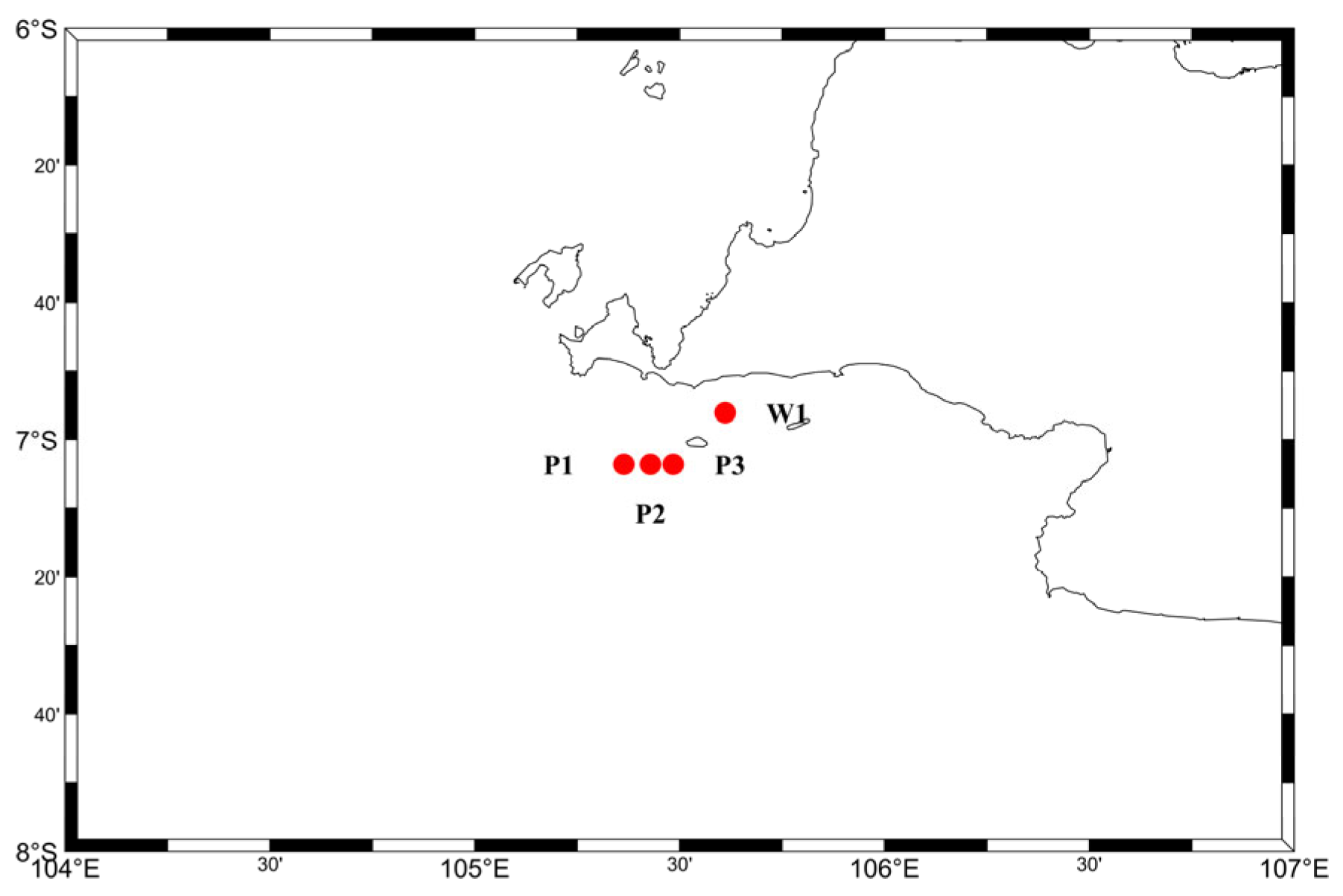
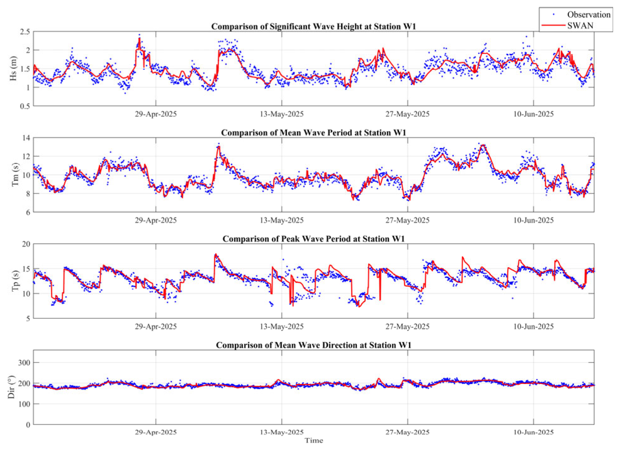
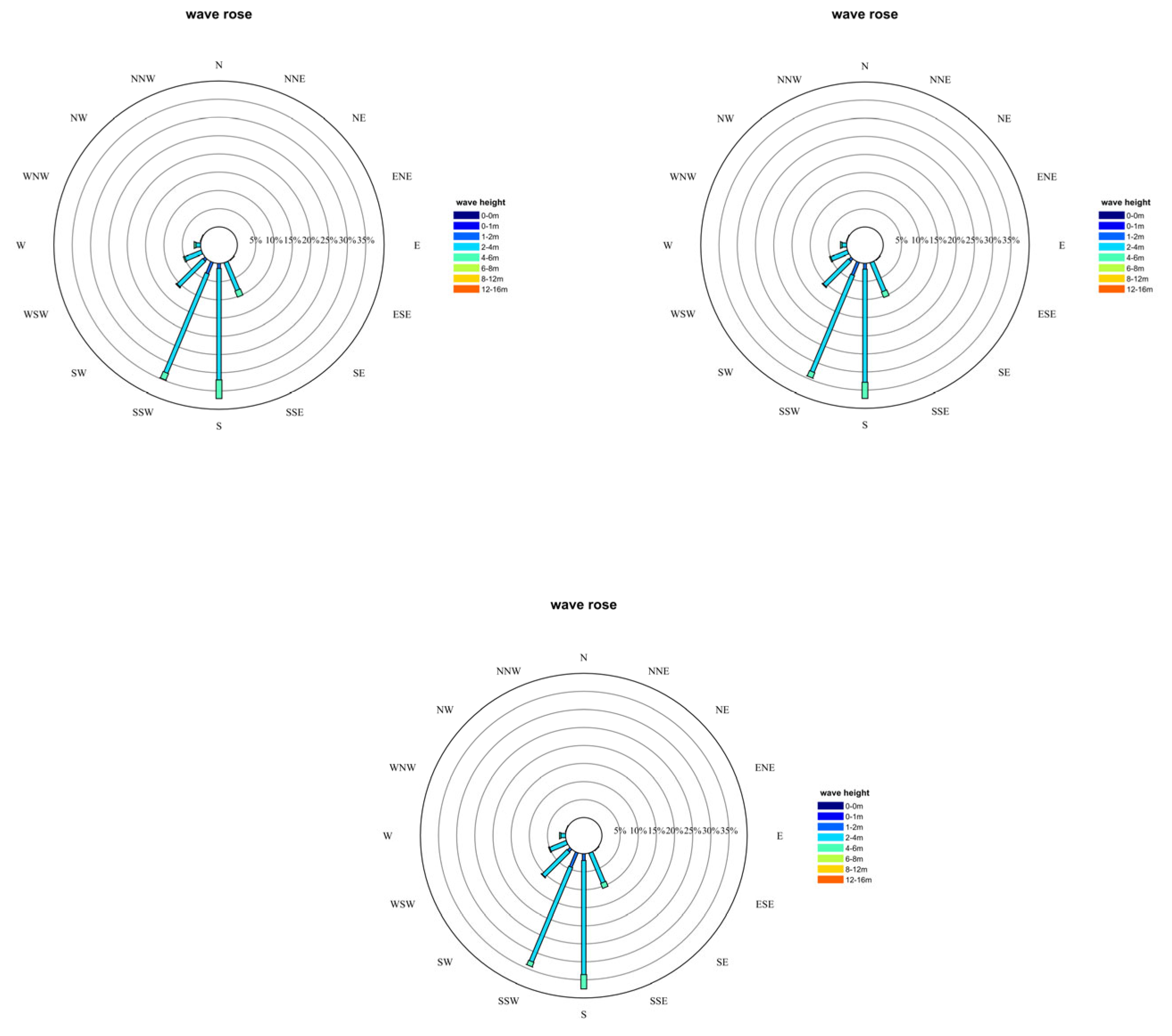
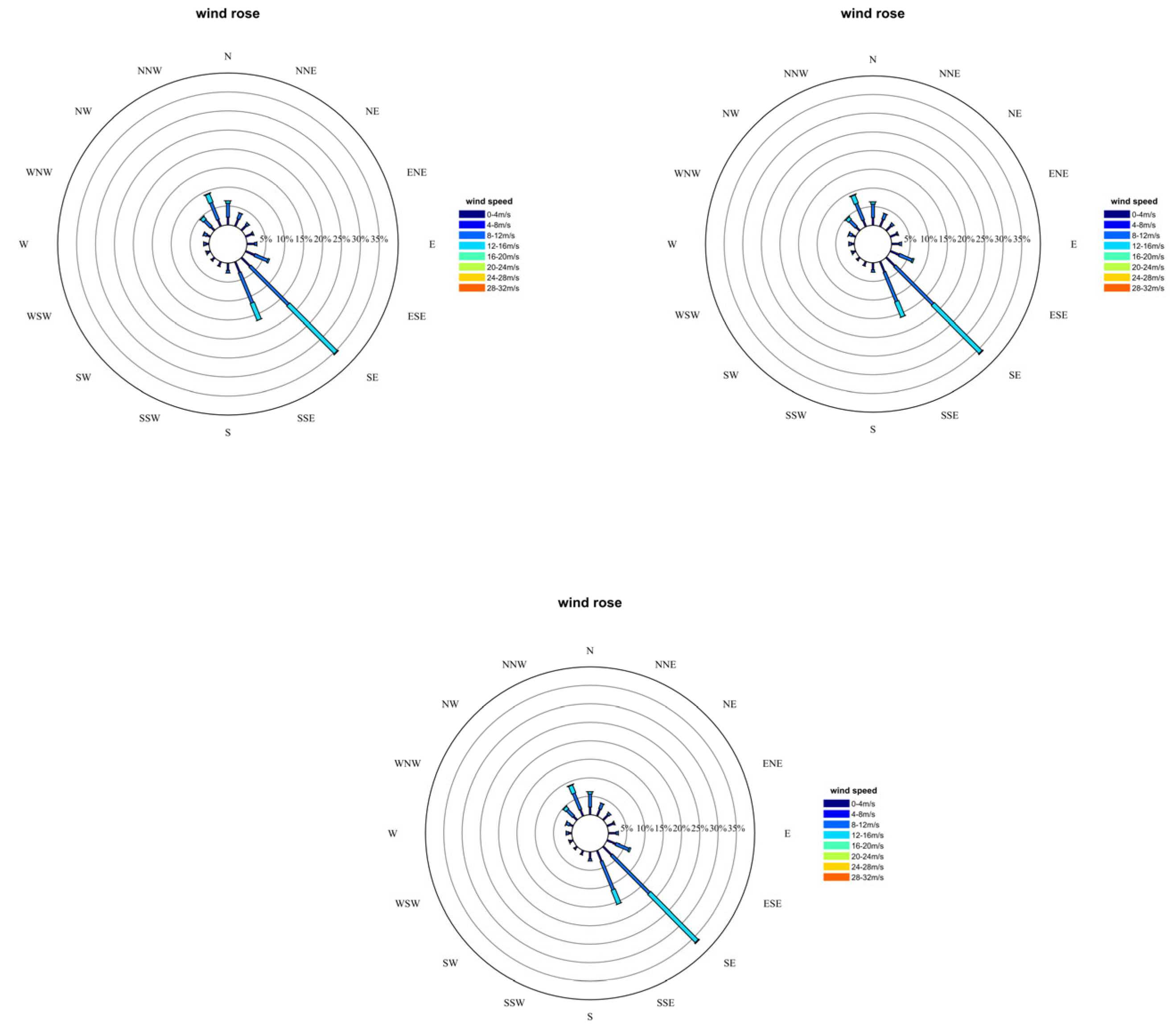
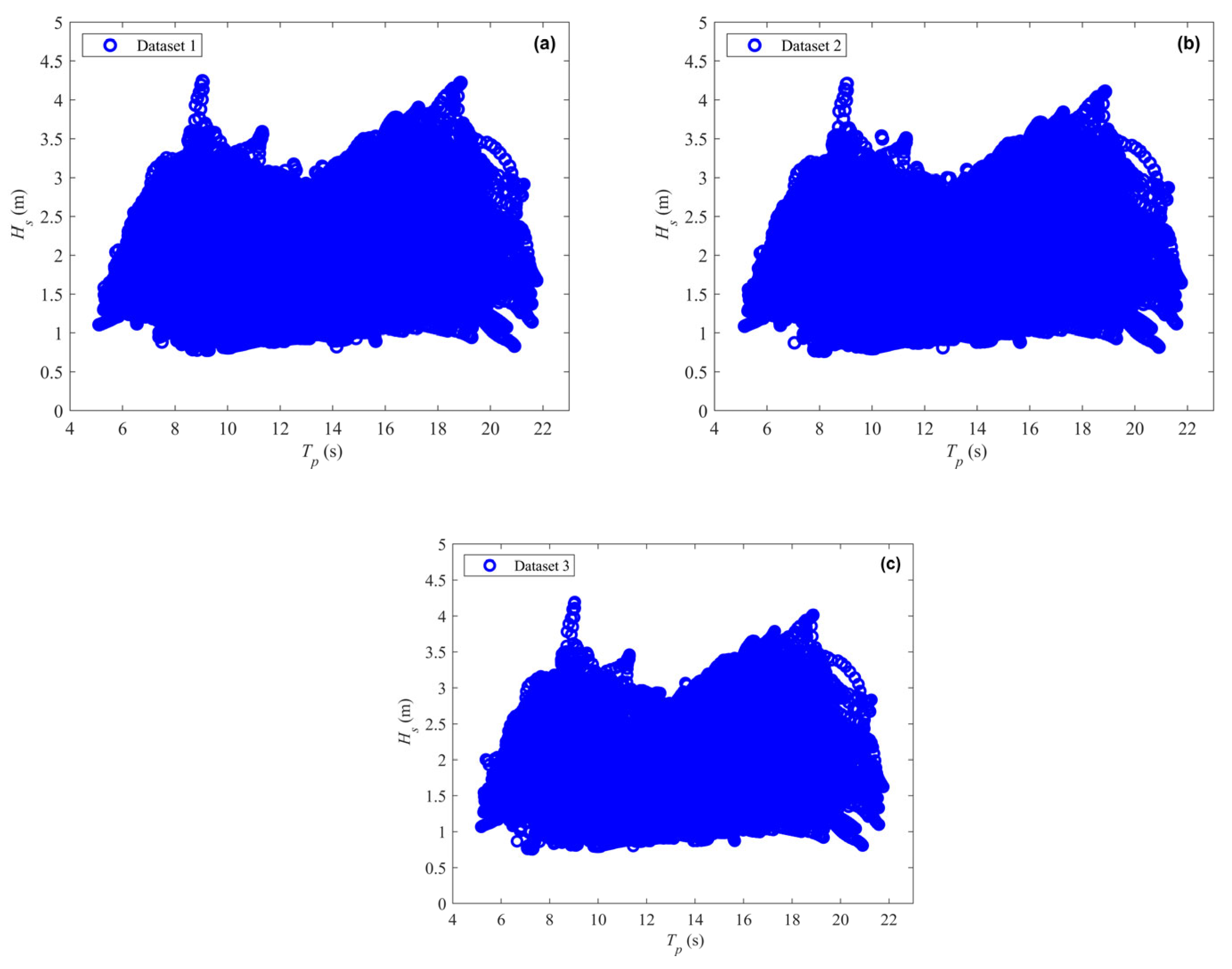
The three selected locations represent similar wave climate regimes within Indonesian waters, positioned in a transitional zone where both swell-dominated and wind-sea-dominated conditions occur with comparable frequencies. Hourly wave data were generated through numerical hindcasting using the SWAN model (version 41.31), forced by ERA5 wind fields (0.25° × 0.25° spatial resolution, hourly) and GEBCO bathymetry (30-arc-second resolution). The hindcast covers 30 years (1996–2025) at three locations, and the SWAN model configuration is listed in Table 2. To validate the hindcast, simulated wave data were compared against available buoy measurements; the geographic positions of the three model locations relative to the measured sites are shown in the new Figure 1, and the validation results are presented in Figure 2 and Table 3. To quantitatively classify the wave regimes, the dimensionless wave age parameter β = Cp/U10 is adopted, where Cp is the peak phase speed and U10 is the wind speed at 10 m height. Following established criteria, 0.8 ≤ β ≤ 1.2 represents mixed/transitional conditions. For the three locations, the 30-year average β values are 1.05 (Location 1), 1.04 (Location 2), and 1.05 (Location 3). The wave and wind roses are presented in Figure 3 and Figure 4. Scatter plots of the wave observations at the three locations are presented in Figure 5. The joint distributions of Hs and Tp exhibit notable differences across the three sites, reflecting the distinct underlying wave generation mechanisms. In contrast to typical wind-sea-dominated datasets, which usually display a relatively narrow and unimodal cloud of points, the scatter plots at all three locations reveal more complex patterns. All three datasets exhibit clear multimodal joint distributions and are representative of mixed wind-swell regimes. The wave/wind roses show comparable directional spread and seasonal patterns. Thus, they are considered as three instances of the same general mixed-sea phenomenon, allowing a consistent evaluation of the GMM-IFORM across varying degrees of swell/wind-sea interaction.
Basic statistical properties of the three datasets are summarized in Table 4. For each location, the mean, standard deviation, maximum value, skewness, and kurtosis are calculated separately for Hs and Tp. The mean significant wave height ranges from 1.82 m to 1.88 m across the three sites. The maximum observed Hs values exceed 4.0 m at all locations, indicating the presence of energetic sea states during extreme events. Skewness and kurtosis provide important insights into the shape characteristics of the marginal distributions. Positive skewness values for Hs at all three locations indicate an asymmetric distribution with a longer upper tail, which is typical for wave height data where extreme events are relatively infrequent but can reach substantial magnitudes. The kurtosis values for Hs are consistently above 3, suggesting heavier tails than a Gaussian distribution. This tail heaviness has direct implications for extreme value estimation, as it indicates a non-negligible probability of encountering severe sea states. For Tp, the statistical characteristics exhibit greater variability across locations. All locations display negative skewness, reflecting a distribution with a longer lower tail. The kurtosis values for Tp also similar, which corresponds to the multimodal structure observed in the scatter plot. This multimodal characteristic is further corroborated by the relatively large standard deviations in Tp, indicating a broad range of wave periods. The distinct statistical properties of the three datasets, particularly the presence of multimodal joint distributions and complex dependence structures, make them well-suited for evaluating the performance of the GMM against conventional conditional joint distribution approaches. The following sections present the implementation of environmental contour construction using both methods, with a focus on their ability to accurately represent the underlying probabilistic characteristics of the wave data.

4.1. Conditional Joint Distribution

The conditional joint distribution approach relies on an accurate specification of the marginal distribution of significant wave height [35]. In this study, a three-parameter Weibull distribution is employed to fit the marginal distribution of Hs for each of the three Indonesian locations. The estimated parameters are listed in Table 5. The fitting performance of the cumulative probability is illustrated in Figure 6, where the empirical cumulative distribution functions derived from the observed data are compared with those estimated using the three-parameter Weibull model.
As can be observed from Figure 6, the three-parameter Weibull distribution provides a reasonable approximation for the central portion of the wave height distribution across all three locations. However, notable deviations between the observed and fitted curves become evident in the upper tail regions, which are of particular importance for extreme value estimation and design sea state assessment. At Location 1, where the wave climate is dominated by swells, the fitted Weibull model tends to underestimate the cumulative probabilities for higher Hs values, indicating that the model fails to capture the extended upper tail characteristic of the observed data. A similar pattern is observed at Locations 2 and 3, which exhibits transitional wave conditions, where the discrepancies in the upper tail are also pronounced. These discrepancies suggest that the three-parameter Weibull distribution, despite its widespread use and mathematical convenience, may not offer an ideal fit for the entire marginal distribution of Hs, particularly in regions where mixed wave systems, such as the coexistence of wind seas and swells, give rise to more complex distributional shapes. In practical terms, underestimation of the upper tail probabilities can lead to unconservative predictions of extreme wave heights for long return periods. While such underestimation may reduce the estimated design loads on floating wind turbines, it introduces potential risks to structural reliability under actual sea conditions. Accurate characterization of the tail behavior is therefore essential for ensuring both safety and economy in marine structure design. The limitations observed in the marginal fitting further underscore the necessity of adopting more flexible modeling frameworks. In the following sections, the GMM is introduced as an alternative approach capable of capturing the full range of the wave height distribution, including its tail behavior, with greater fidelity.
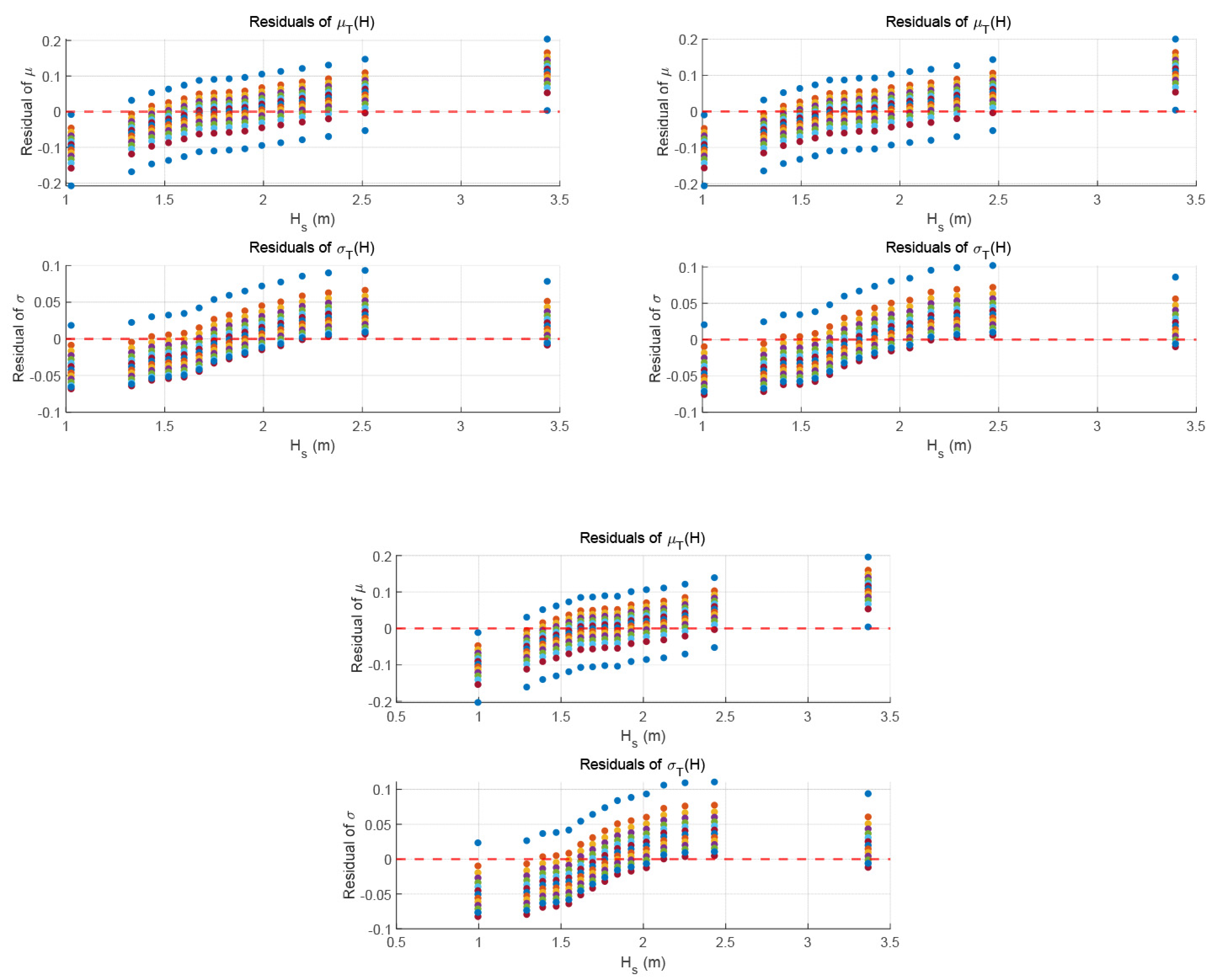
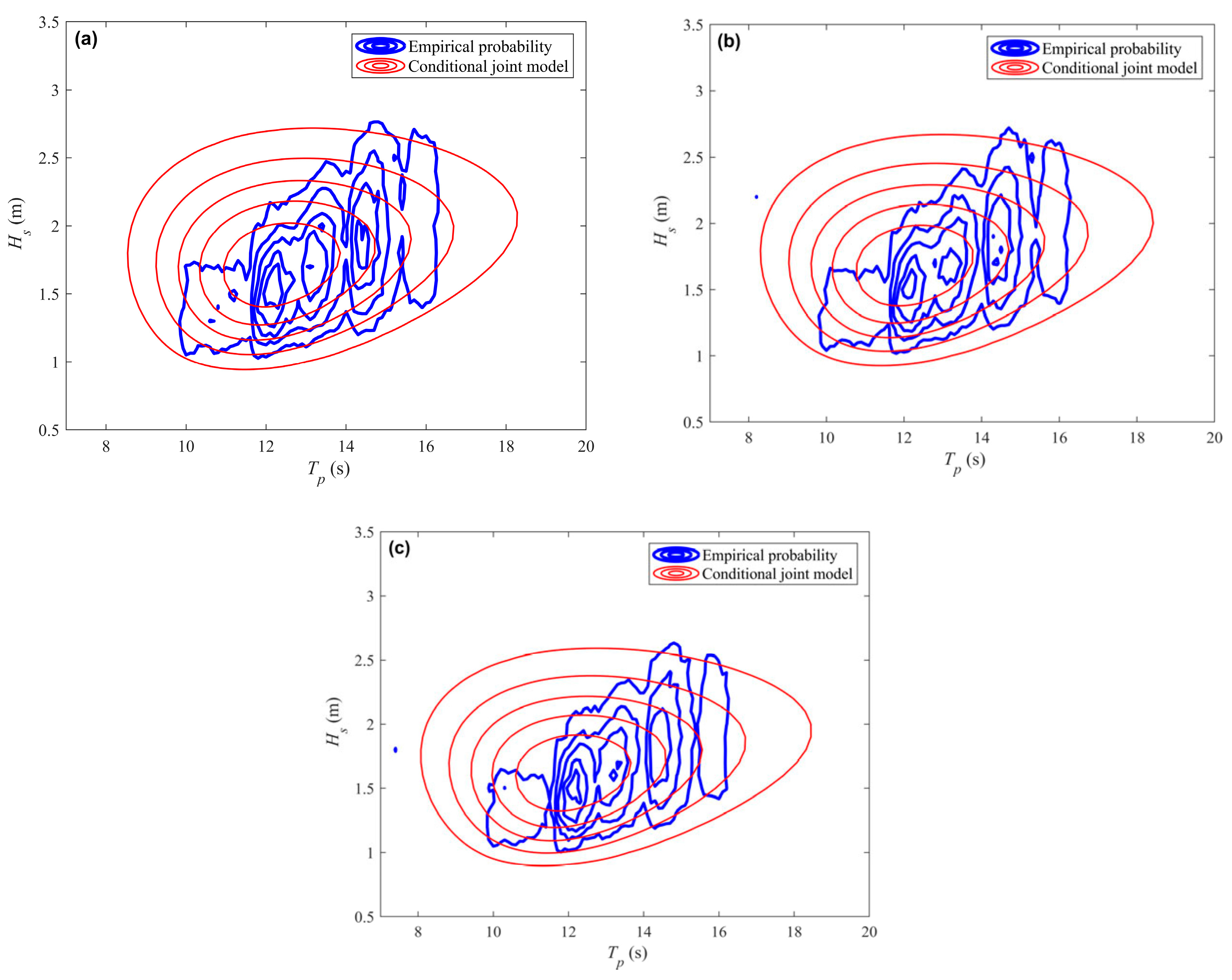
The conditional joint distribution approach, formulated as the product of the marginal distribution of Hs and the conditional distribution of Tp given Hs, is employed to model the joint behavior of wave observations at the three Indonesian locations. A three-parameter Weibull distribution is applied to characterize the marginal distribution of Hs, while a lognormal distribution is used to model Tp conditional on Hs. 15 bins over the range of Hs, with the conditional mean and standard deviation of ln(Tp) computed within each bin. The conditional parameters, namely the expectation μ and standard deviation σ of lnTp, are expressed as quadratic functions of Hs. The coefficients of these quadratic functions are estimated for each location using nonlinear least squares regression, and the results are summarized in Table 6. The fitted curves for μ and σ as functions of Hs are presented in Figure 7 for all three locations, which was performed using the MATLAB2023b Curve Fitting Toolbox. Regression residuals for µ(Hs) and σ(Hs) shown in new Figure 8. As can be observed, the quadratic functions provide a general representation of the trend in the conditional parameters; however, considerable scatter exists around the fitted curves, particularly at higher wave heights. This scatter indicates that the relationship between Tp and Hs is not adequately captured by a simple second-order polynomial, suggesting more complex dependence structures that vary across different wave regimes. Using the estimated conditional model, the bivariate joint probability density of (Hs, Tp) is constructed. Density contour plots derived from the conditional joint model are presented in Figure 9 alongside empirical density contours, which are obtained by aggregating the observed data into a joint histogram with cell sizes of 0.1 m × 0.1 s.
As evident from Figure 9, the density contours generated by the conditional joint model exhibit notable discrepancies from the empirical contours across all three locations. At all locations, where multimodal patterns are present in the empirical data, the conditional model produces a unimodal distribution that fails to capture the distinct swell and wind-sea populations. The model contours appear overly smooth and fail to reflect the complex multimodal structure inherent in the observed wave data. The conditional model struggles to capture the extended tail behavior and the more diffuse structure evident in the empirical contours. Deviations persist in the upper tail region where extreme wave heights and associated periods occur.
The observed discrepancies can be attributed to two primary factors. First, as discussed in Section 4.1, the three-parameter Weibull distribution does not adequately represent the upper tail of the marginal distribution of Hs, leading to biased estimates in the extreme value region. Second, the conditional lognormal model, with its assumed quadratic functional forms for μ(h) and σ(h), imposes a restrictive structure on the dependence between wave height and period. This limitation becomes particularly pronounced when the underlying dependence is nonlinear, heteroscedastic, or multimodal, features that are characteristic of mixed sea states involving coexisting wind seas and swells. The inability to accurately capture these complex dependence patterns results in substantial deviations in the resulting joint density contours, particularly in the tail regions that are most critical for design sea state assessment.

4.2. Gaussian Mixture Distributions

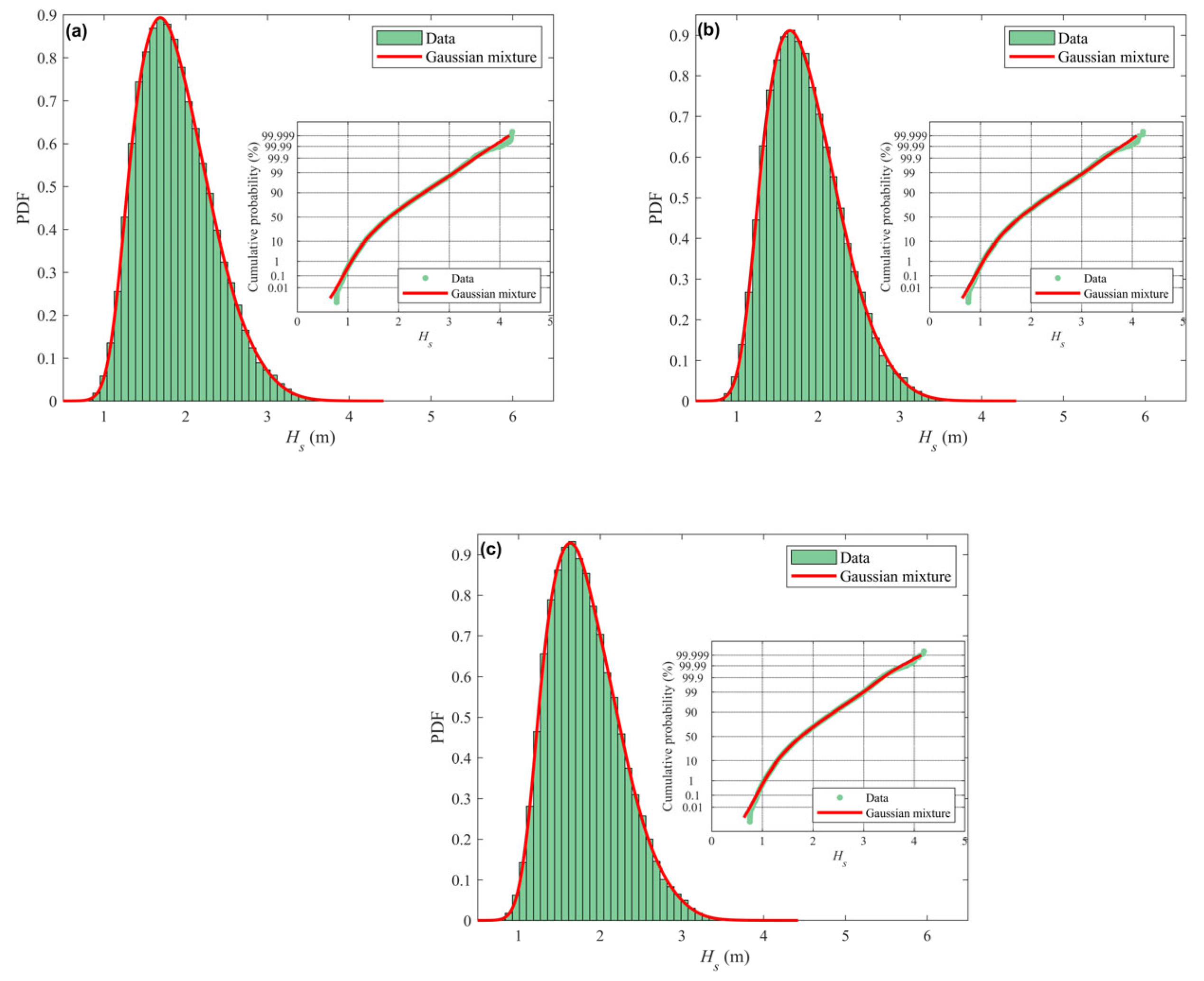
Given that the conditional joint model fails to adequately capture the complex characteristics of wave data from regions with mixed wind and swell conditions, the GMM, constructed as linear combinations of univariate or multivariate Gaussian distributions, is employed as an alternative approach to characterize the distributional patterns of wave parameters. In this study, a univariate GMM is first applied to fit the marginal distribution of significant wave height Hs. The fitting performance of the mixture model for the marginal distribution is illustrated in Figure 10, where the probability density function and cumulative distribution function estimated from the GMM are compared with the empirical distributions derived from the observed data. As can be observed from Figure 10, the GMM provides a significantly improved representation of the marginal distribution of Hs compared to the three-parameter Weibull model discussed in Section 4.1. The mixture model captures both the central tendency and the tail behavior with greater fidelity. The improved marginal fitting achieved by the GMM lays a solid foundation for the subsequent construction of bivariate environmental contours. In the following section, the bivariate GMM is employed to capture the joint distribution of (Hs, Tp) and to derive environmental contours for design sea state assessment. To further quantify the upper-tail behavior, we provide Q-Q plots (Figure 11) comparing the empirical quantiles of Hs against the fitted three-parameter Weibull quantiles. Return-level comparisons between the Weibull model and the Gaussian mixture model are presented in Figure 12, and tail RMSE values computed for the upper 5%, 10%, 15%, and 20% of the data are summarized in Table 7. These quantitative assessments clearly demonstrate that the Weibull model consistently underestimates the upper-tail probabilities, whereas the GMM provides a much closer fit. Quantitative uncertainty bands for the tail estimates (e.g., confidence intervals for return levels or exceedance probabilities) are not provided; this is a limitation of the current study. Future work should incorporate such uncertainty quantification to further strengthen the tail comparison.
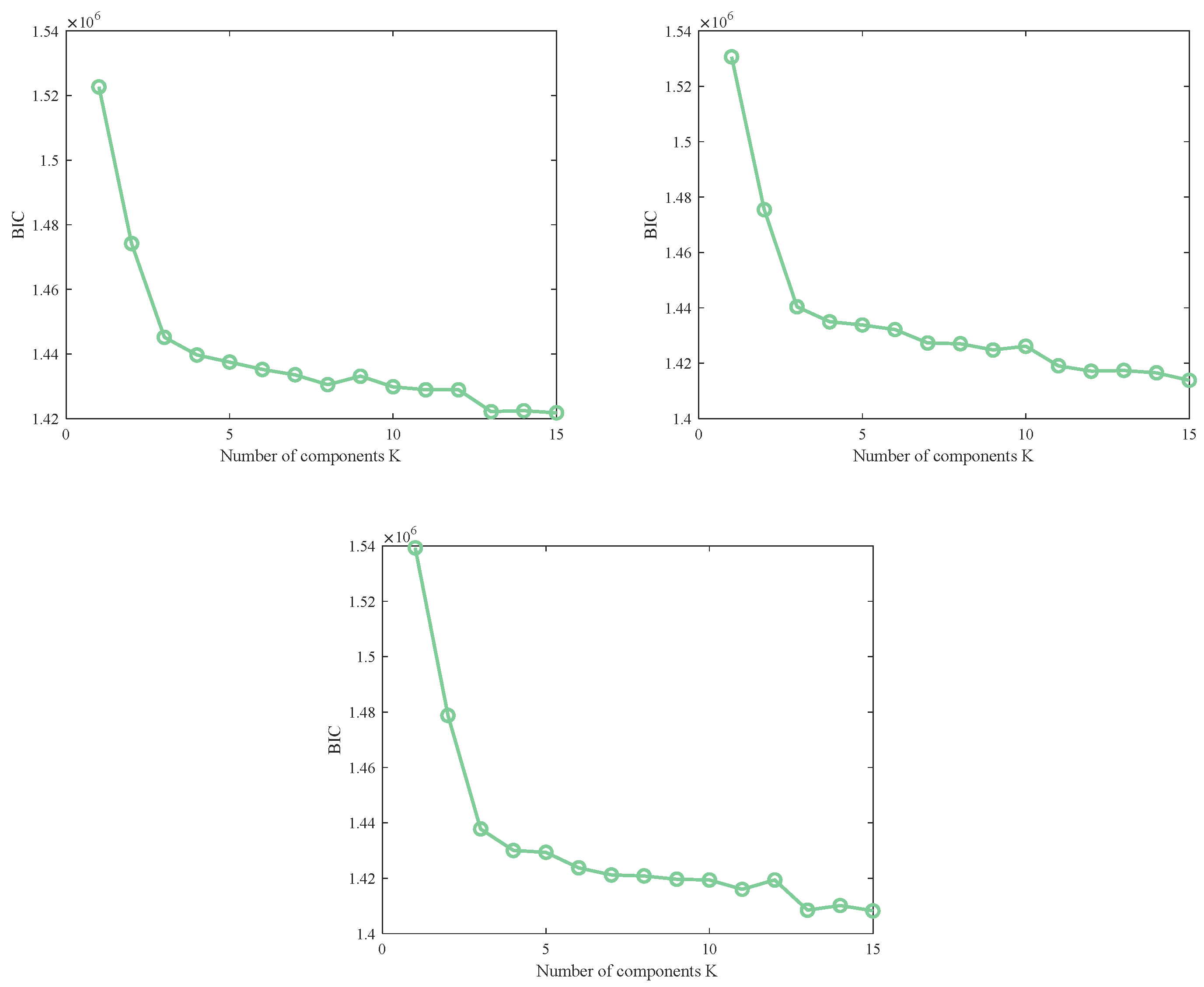
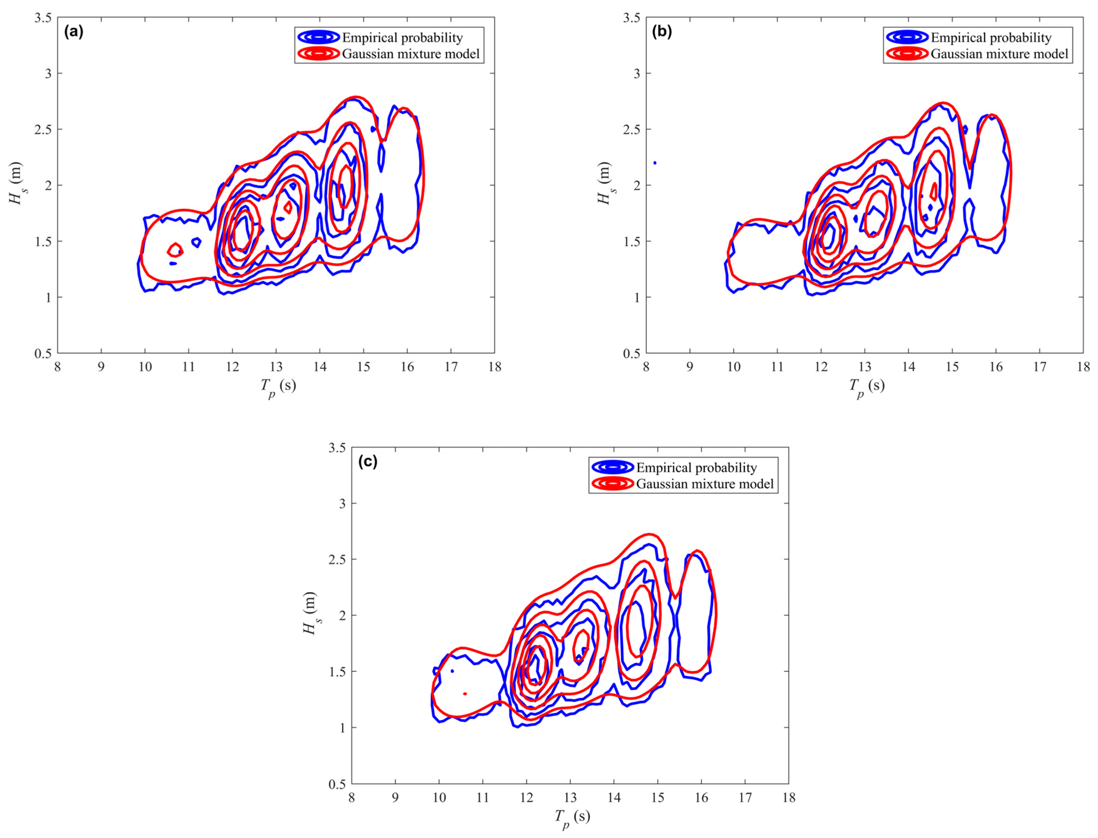
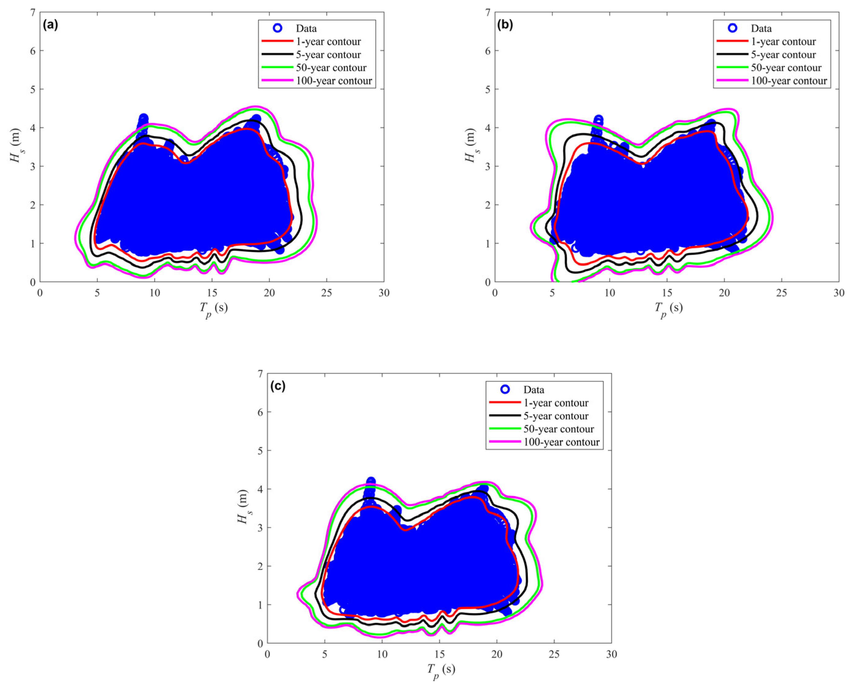
The optimal number of mixture components for each location is determined based on the BIC, which balances model fit against complexity. The calculated BIC values for different numbers of components, along with the selected optimal component numbers, are summarized in Table 8. Figure 13 shows the BIC curves for K = 1 to 15, confirming that the minimum occurs at K = 14–15 for all three locations. To avoid overfitting, the EM algorithm was implemented with full covariance matrices, k-means++ initialization (ten repeated runs), a regularization constant of 1 × 10⁻⁶ on covariance diagonals, and convergence declared when the log-likelihood change fell below 1 × 10⁻⁶ (or after 1000 iterations). These settings ensure that the high component numbers capture genuine multimodal structure rather than noise. With the EM algorithm, training on ~260,000 hourly samples with K = 15 converges in approximately 40 s on a standard desktop (Intel i7, 16 GB RAM). Once fitted, generating a 200 × 200 PDF grid and extracting contours takes less than 2 s. The density contours derived from the bivariate GMM are presented in Figure 14 alongside the empirical density contours obtained from the observed data. As clearly observed from Figure 14, the bivariate GMM exhibits a high degree of concordance with the empirical joint distribution across all three Indonesian locations. Compared to the conditional joint model presented in Section 4.1, the GMM offers several distinct advantages. First, it allows the data itself to determine the underlying components. Second, it naturally accommodates multimodal distributions that arise from mixed sea conditions, which conventional models struggle to represent. Third, it provides consistent modeling of both marginal and joint characteristics within a unified framework, ensuring that the fitted distribution accurately reflects the empirical probability structure across the entire range of the data. It is worth noting that although Gaussian components assign small but non-zero probability to physically unrealistic negative values of Hs and Tp, we truncate the fitted distributions at zero and renormalize, which introduces negligible error. For all three locations, the integrated probability over the range (−∞,0) for Hs is less than 1 × 10⁻⁶, and for Tp it is less than 5 × 10⁻⁶. After truncation at zero and renormalization, the relative change in key quantiles is below 0.01%, confirming that the effect is negligible. The improved fitting performance of the GMM is particularly evident in the tail regions, which are of critical importance for design sea state assessment. While the conditional joint model exhibited systematic deviations in the upper tails of both marginal and joint distributions, the mixture model maintains a close agreement with empirical probabilities even at extreme values. This capability is essential for reliable estimation of return periods and extreme responses in marine structure design.

4.3. Distribution Models Assessment

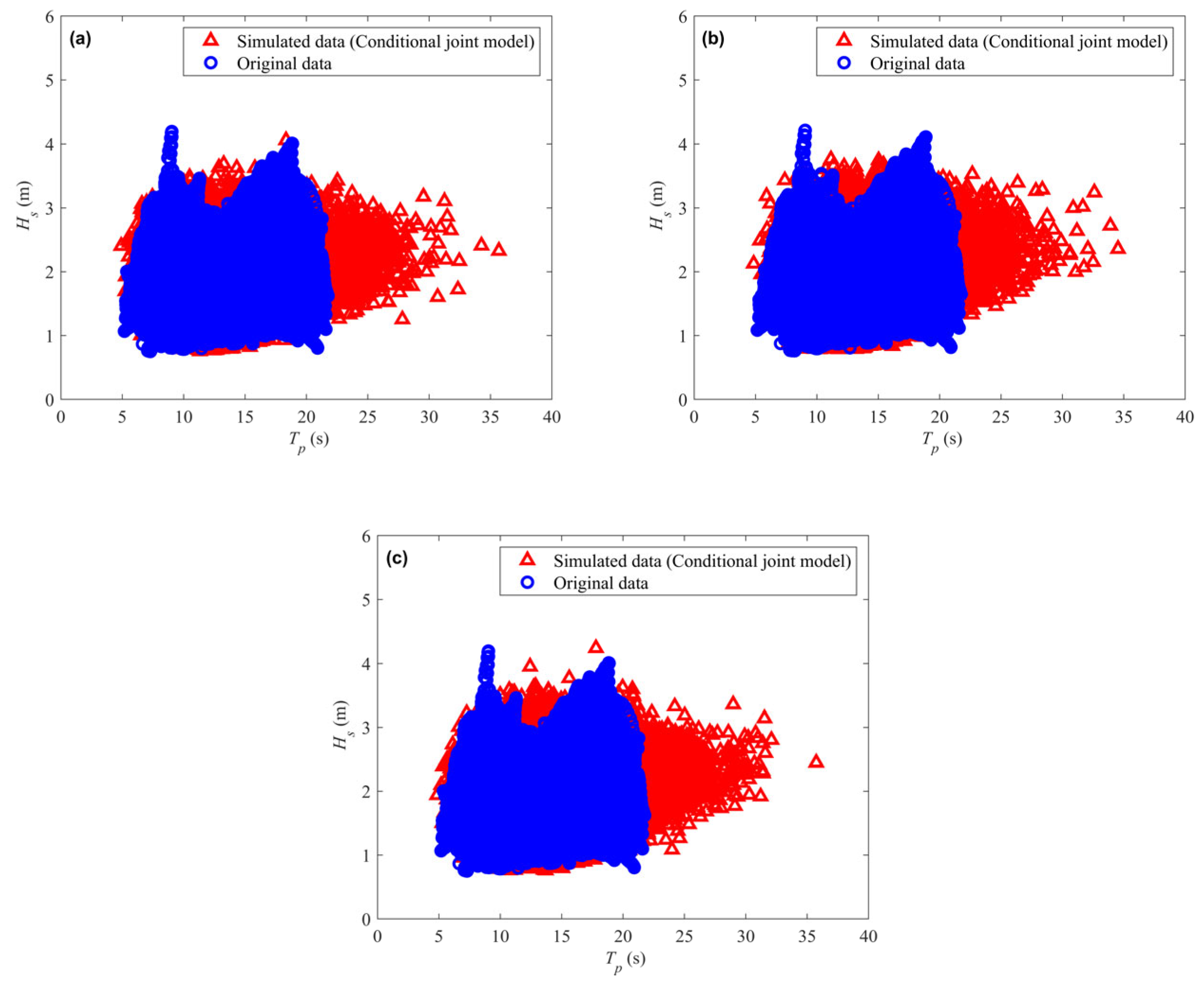
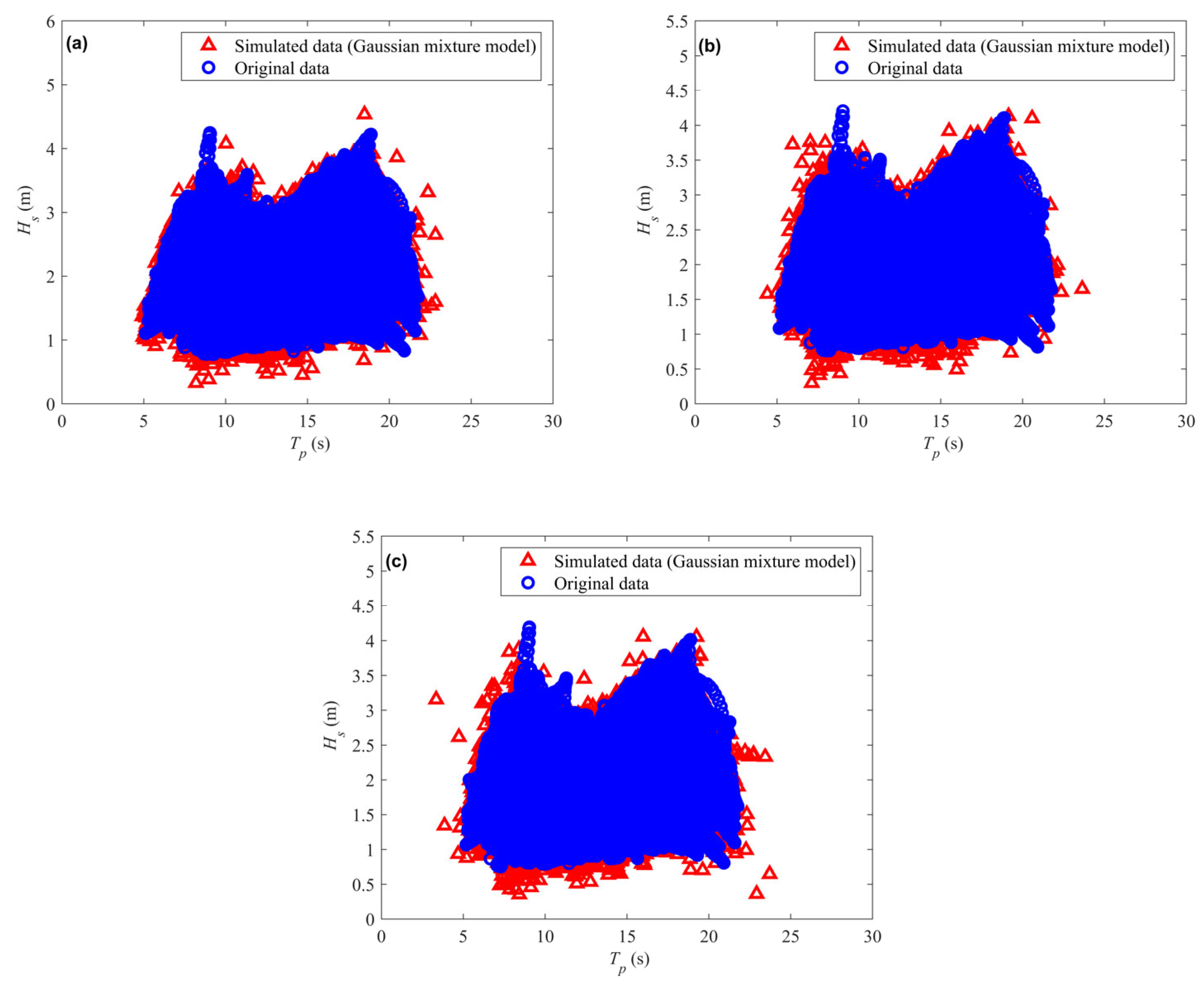
The performances of the conditional joint distribution and the Gaussian mixture distribution are further evaluated by comparing simulated data with the original observations. To facilitate this comparison, random variables are generated following the candidate joint probability density functions. Monte Carlo simulation is employed to produce discrete random wave data, and the inverse transform method is applied for random variable simulation, given that the marginal and joint distributions of the wave parameters are properly defined. For reproducibility, the random seed was fixed to 42 (rng(42)). Initially, 100,000 uniformly distributed random samples (z1, z2) are generated. We repeated the simulation with 10,000, 50,000, 100,000, and 500,000 samples. The tail statistics (e.g., the 95th percentile of Hs) showed a relative change of less than 2% when increasing the sample size from 100,000 to 500,000. Subsequently, random environmental variables are transformed as x 1 = F X 1 1 ( x 1 ) and x 2 = F X 2 | X 1 1 ( z 2 | x 1 ) for the conditional model, while for the GMM, random samples are drawn directly from the fitted mixture distribution using the random method. For all three locations, every generated sample fell within the physically admissible range (Hs > 0, Tp > 0), and a sensitivity analysis confirmed that 100,000 samples provide stable tail statistics (relative change < 2% compared to 500,000 samples). In the Monte Carlo simulation, we sampled directly from the fitted GMM without explicit truncation. Given that environmental contours focus on extreme sea states (large Hs and Tp), this negligible negative tail has no practical effect on the contour estimates. Therefore, we treated the negative probability mass as numerically negligible and did not apply truncation in the sampling step. Scatter plots of the original observations and simulated realizations from the conditional joint distribution and GMM are presented in Figure 15 and Figure 16, respectively, providing a visual assessment of the fitness of various joint models to the measured data. As can be observed from Figure 16, the GMM yields reasonable simulations that exhibit good agreement with the empirical data across the entire range of wave conditions. The simulated data points effectively replicate the joint distribution characteristics of the original observations, including the multimodal structure and the extended tail behavior observed at all three locations. In contrast, as shown in Figure 15, the simulated variables from the conditional joint distribution fail to fully describe the entire original dataset. Considering the complex dependence structure in datasets from locations with mixed wind and swell conditions, the mixture model provides a more accurate description of the dependence compared to the conventional conditional joint model. The ability of the GMM to capture the bimodal patterns and complex dependence structures is clearly reflected in the simulated scatter plots, which closely mirror the empirical data distribution. The results of random variable simulation based on the two candidate models are consistent with the joint probability density plots shown in Figure 9 and Figure 14, further validating the superior performance of the mixture model in representing both ordinary and extreme sea states.

Error Metrics

Beyond the qualitative inspection using scatter plots, a quantitative goodness-of-fit analysis was performed, and error statistics were derived to appraise the two joint probabilistic models. Two commonly adopted accuracy indicators, RMSE and R2, were employed to evaluate the discrepancies between empirical observations and theoretical distributions. A model with a smaller RMSE is generally preferred, and an R2 value approaching unity signifies a closer alignment between the measured data and model predictions. Fi is the empirical copula value C(Ui, Vi), where Ui = FH(Hi) and Vi = FT(Ti) are obtained via the empirical marginal distributions. F ^ i are computed from the fitted GMM and conditional models, respectively, for the GMM, F ^ i = k = 1 K π k Φ ( ( H s i , T p i ) ; μ k , Σ k ) ; for the conditional Weibull–Lognormal model, F ^ i = F H s ( H s i ) F T p | H s ( T p i | H s i ) . Table 9 reports the computed error metrics. For each of the three datasets, the GMMs yield R2 values nearly equal to 1.0000, reflecting an exceptionally strong correspondence between actual and estimated values. Clearly, the GMMs achieve markedly lower RMSE values and therefore demonstrate a considerably better fit than their conditional counterparts. In comparison with the conditional modeling technique, the GMMs offer a substantially improved representation of the bivariate behavior of wave parameters. The RMSE values computed over the upper 5%, 10%, 15%, and 20% of the data are listed in Table 10. Additionally, a hold-out validation (70% training/30% testing) was performed to reassess the models on independent data. The RMSE and R2 were recomputed on the testing set using the same empirical CDF definition, and the log-likelihood values on the testing set are presented in Table 11. We have performed 5-fold cross-validation for the GMM fitting. Specifically, each dataset was randomly split into five folds; four folds were used for training (EM algorithm with BIC-selected number of components) and the remaining fold for testing. This process was repeated five times, ensuring that every data point appears once in the test set. The average test-set log-likelihood and tail RMSE (upper 10% tail) were very close to the training-set values across all folds, indicating that the relatively high number of components (K = 14–15) captures genuine structure rather than overfitting noise. Detailed per-fold results are presented in Table 12.
The accurate modeling of marginal distributions for significant wave height is critical, as it directly indicates the severity of sea states, especially for extreme sea condition estimation. To evaluate the performance of the adopted models, the three-parameter Weibull distribution and the GMM, univariate goodness-of-fit tests were conducted using both the KS and chi-square criteria. The test is performed using MATLAB’s built-in chi2gof function, which automatically divides the data into a number of bins (chosen to be equiprobable under the fitted distribution) and applies a default binning strategy that ensures an expected count of at least 5 in each bin; the actual number of bins is printed in the output. The degrees of freedom are automatically corrected as df = number of bins−1−number of estimated parameters. For Dataset 2, the GMM gave a χ2 statistic of 16.31 with df = 9, which corresponds to a p-value of approximately 0.06. Since this p-value is greater than 0.05, the null hypothesis (that the data come from the fitted GMM) cannot be rejected at the 5% significance level. The conditional model, by contrast, gave a χ2 of 4.87 × 10³ with a p-value < 0.001, leading to rejection of the null hypothesis and indicating a clearly worse fit. To assess sensitivity to binning, we repeated the test with 8, 10, and 12 manually specified bins; the p-value for the GMM remained above 0.05 in all cases, confirming the robustness of the GMM fit. Table 13 summarizes the resulting statistics for the three datasets. In this table, an “(F)” mark denotes that the test statistic exceeds the corresponding critical value, implying that the theoretical distribution fails the GOF test. For all three datasets, the three-parameter Weibull distribution exhibits KS values (0.0255, 0.0272, 0.0332) larger than the critical value (0.0026) and χ2 values (4.66 × 10³, 4.87 × 10³, 5.71 × 10³) far above the respective thresholds (15.51), thus failing every test. In contrast, the GMM yields KS statistics (0.0010, 0.0015, 0.0011) below the critical value and χ2 statistics (13.63, 16.31, 13.65) under the critical values (16.92 for all three, given 9 degrees of freedom), thereby passing all GOF tests. It is worth noting that the extremely small KS critical value arises from the large sample sizes, making the test stringent. These results indicate that the measured significant wave height records are not well represented by the conventional three-parameter Weibull distribution; its use could introduce substantial statistical errors in fitting Hs and subsequently in estimating extreme wave loads. From the perspective of both the KS and χ2 tests, the GMM offers a superior and reliable fit for the marginal distribution of Hs.

4.4. Environmental Contour

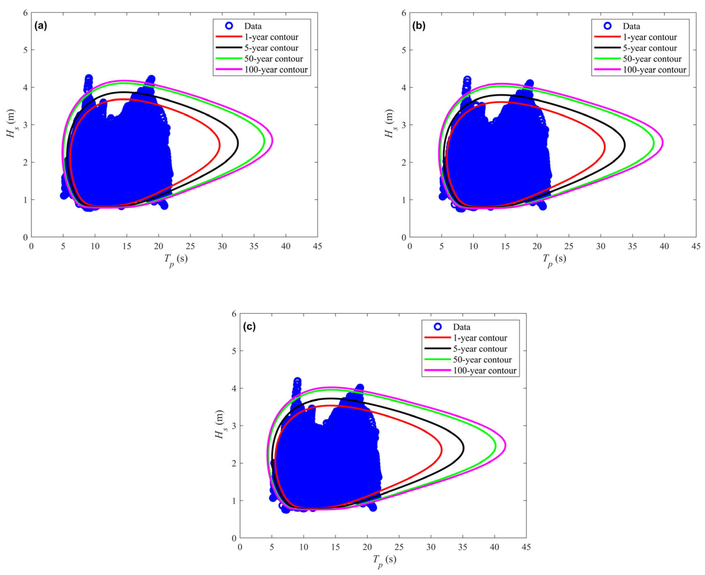
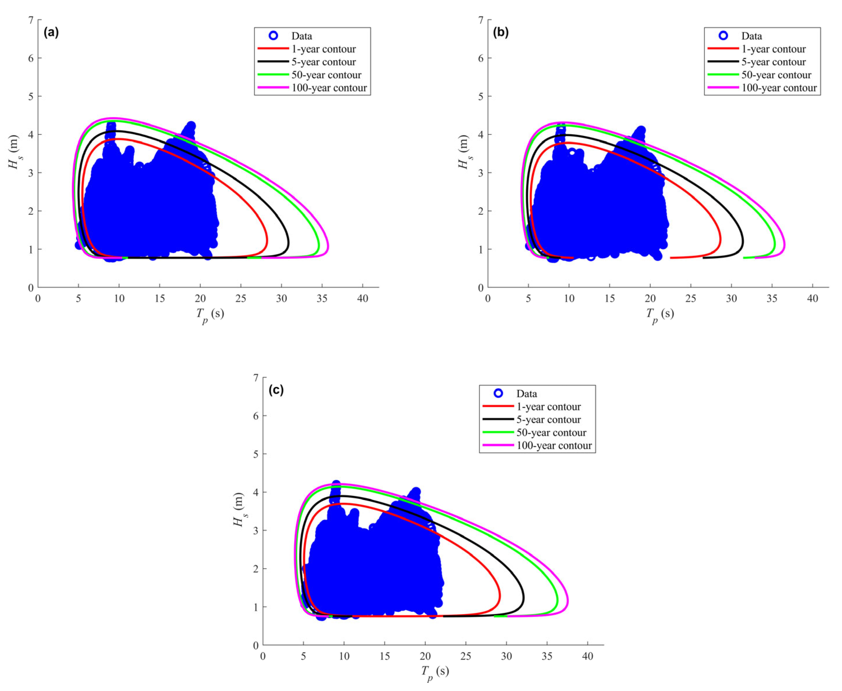
Environmental contours serve as a standard tool for providing representative or extreme ocean parameters in the design load calculation and damage assessment of marine structures. To accurately apply the environmental contour method for structural response evaluation, it is essential to develop reliable probabilistic models that can faithfully represent the joint behavior of metocean variables [36]. Sea-state duration is 1 h (hourly observations). Hourly sea states are treated as independent for the purpose of return-period definition, which follows standard practice (DNV [30]). The average number of independent sea states per year is λ = 365 × 24 = 8760. If one wishes to account for serial dependence, the work of Vanem on the effect of serial dependence in environmental contours can be consulted [25]. The return-period exceedance probability for a contour is computed as Pf = 1/(N·λ), and the corresponding probability level for the contour is set equal to Pf. The reliability index is then β = Φ−1(1 − Pf), where Φ−1 is the inverse standard normal CDF. The environmental contour in the standard normal space is a circle of radius β: u1 = βcosθ, u2 = βsinθ, with θ discretized into 360 equally spaced angles. For each θ, the point in the physical space (Hs, Tp) is obtained via the Rosenblatt transformation using the fitted GMM and conditional joint model. The environmental contours derived from the conventional conditional joint distribution and those generated from the GMM within the IFORM framework are presented in Figure 17 and Figure 18, respectively. These contours correspond to four return periods, 1-year, 5-year, 50-year, and 100-year, which span both moderate and severe sea conditions. A comparison of the two figures reveals that the contours based on the GMM exhibit substantially enhanced performance relative to those obtained from the conventional approach. As illustrated in Figure 18, the GMM demonstrates considerable flexibility in adapting to the underlying structure of the wave data. It effectively determines the appropriate number of components and captures the dependence patterns among them, allowing for a more accurate representation of complex wave characteristics. This adaptability is particularly evident in regions where the scatter plots exhibit multimodality or irregular dependence structures. The slightly irregular/wavy shape of the GMM contours is a numerical artefact caused by the high number of mixture components (K = 14–15) and the local variations in the contour lines; in this case study, it has a slight effect on the estimated extreme sea states. Compared with the conditional Weibull–Lognormal distribution, the GMM provides a more plausible description of severe sea conditions, which are inherently less frequent in the observational record. The contours constructed using the GMM align well with the majority of the measured wave data and follow the trend of the empirical density distribution. In contrast, the contours derived from the conditional joint distribution, shown in Figure 17, appear less reliable when extrapolating to rare extreme events. Substantial gaps exist between the data points and the environmental contours, which exhibit poor alignment in shape and trend. This shortcoming stems from two main limitations: the three-parameter Weibull distribution inadequately captures the upper tail of the wave height distribution, and the conditional lognormal parameters cannot be accurately represented by the assumed quadratic functions. Given that extreme events with low occurrence probabilities are critical for evaluating structural integrity and reliability, the predictive capability of the conditional joint model in the tail region proves insufficient for guiding structural response assessments. Overall, in the tail region, the GMM exhibits a closer correspondence with the empirical density values, suggesting that it can be a suitable framework for constructing environmental contours and estimating extreme sea states. Additionally, we have now compared the GMM contours with those derived from a Gaussian copula with Weibull marginals (Figure 19). The copula-based contours are smoother but underestimate the extreme tail coverage [19]. This work demonstrated improvement in joint distribution fitting under mixed wind-swell conditions compared with Gaussian copula model; a quantitative contour-level validation is recommended for future work.
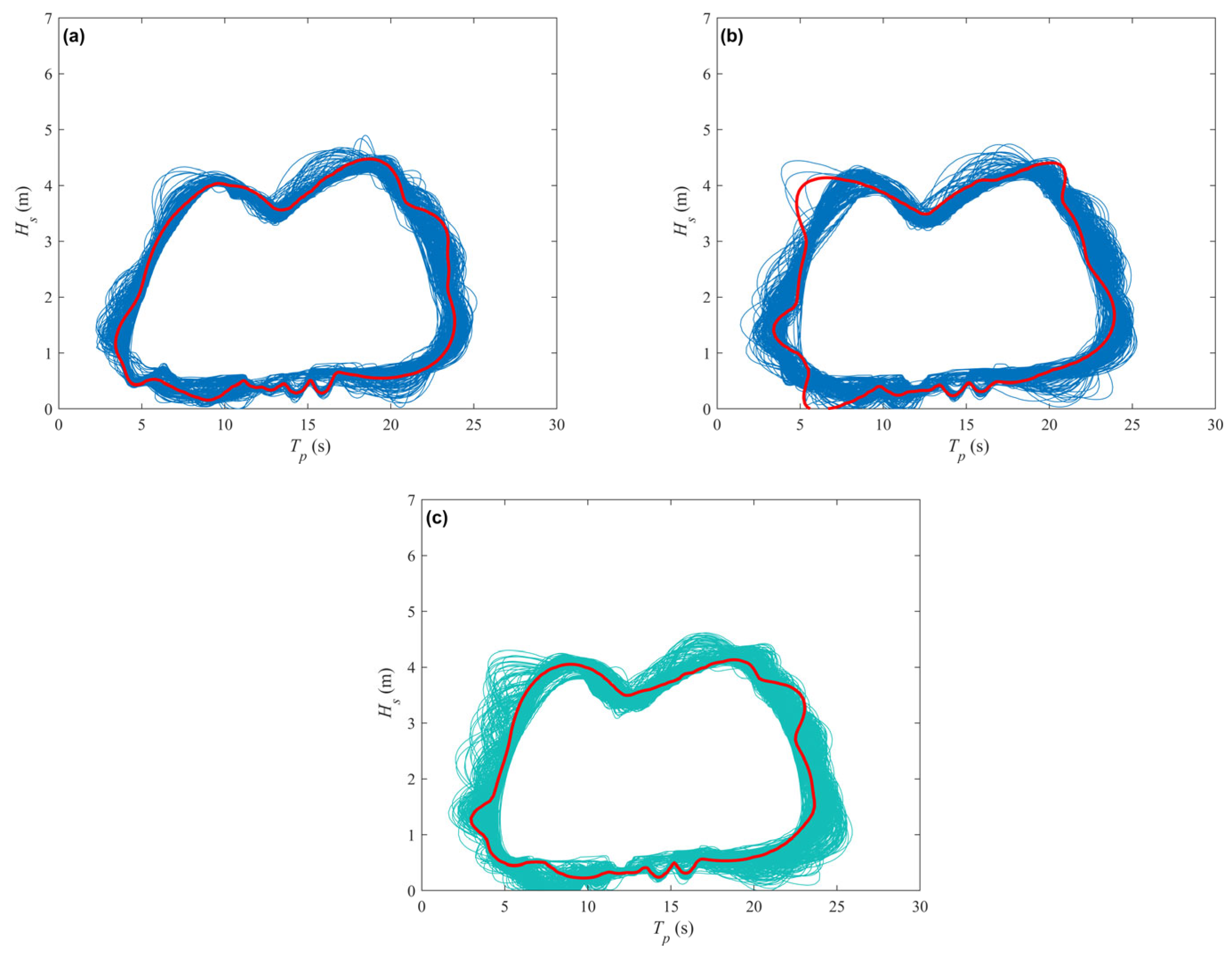
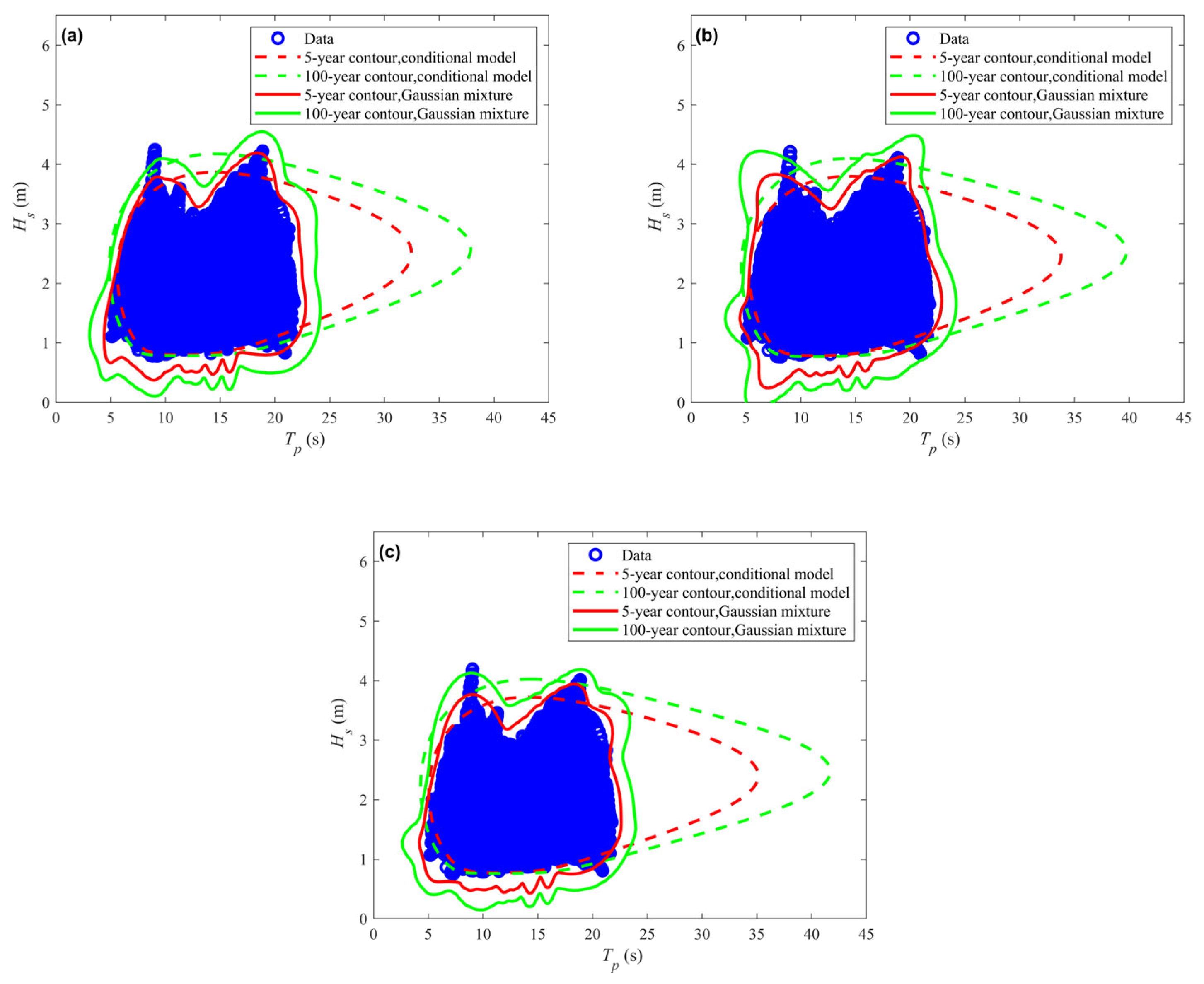
Figure 20 presents the bootstrap results (500 resamples) for the 50-year return period environmental contour derived from the Gaussian mixture model. Specifically, for the 50-year contour, the 95% confidence band width (maximum Hs range) is approximately 0.25 m. The analysis shows that the GMM-based design sea states are stable with a coefficient of variation below 3%, confirming the robustness of the estimated extreme values. Bootstrap uncertainty bands for the 100-year contour are not provided, and this is acknowledged as a limitation of the current study. Figure 21 presents the environmental contours derived from both the conditional Weibull–Lognormal model and the GMM, overlaid on the scatter plots of measured wave data. Contours corresponding to return periods of 5 years and 100 years are shown to facilitate comparison between moderate and extreme sea state conditions. Across all three locations, the GMM shows better agreement with the empirical data distribution in terms of overall shape and trend, and improves distribution fit. For the 5-year return period contours, the GMM effectively covers the regions where the majority of wave observations are concentrated, particularly the zones associated with higher wave heights. In contrast, the contours generated by the conditional joint distribution exhibit noticeable deviations. Substantial gaps exist between the data points and the conditional model contours, with the latter showing relatively poor alignment in shape and trend. This discrepancy becomes more pronounced for the 100-year return period contours. Under extreme sea state conditions, the Weibull–Lognormal model tends to produce contours that deviate further from the empirical distribution, failing to adequately account for the sparse but critical regions that correspond to severe wave events. The GMM, by contrast, maintains a closer correspondence with the tail behavior of the data. The improved performance of the GMM is particularly evident at locations characterized by complex wave regimes. At all locations, where swell and wind-sea components coexist, the mixture-based contours successfully accommodate the multimodal structure observed in the scatter plot. The conditional model, however, yields contours that are overly smooth and do not capture the distinct wave populations.
Table 14 summarizes the design sea states extracted from the environmental contours for each location and return period. In standard practice (e.g., IEC 61400-3-2), the environmental contour method is used to identify extreme sea states; these discrete points along the contour are then employed as input to aero-hydro-servo-elastic simulations, and the environmental condition that leads to the maximum structural response is selected as the design load case. It should be noted that this study only provides the environmental input parameters; a full structural response analysis and design load verification are beyond the scope of the present work. For each model, the maximum significant wave height along the contour and its associated wave period are reported, along with the maximum wave period and its corresponding wave height. The results show that the GMM consistently predicts higher maximum Hs values compared to the conditional model across all locations and return periods. For instance, at Location 1, the 100-year maximum Hs estimated by the GMM is 4.55 m, whereas the conditional model yields 4.18 m. This difference reflects the ability of the mixture model to better capture the upper tail of the wave height distribution. In terms of wave period predictions, the GMM yields larger associated Tp values corresponding to the maximum Hs, indicating that extreme wave heights are more realistically paired with appropriate wave periods under the mixture framework. Conversely, the conditional model produces substantially larger maximum Tp values, with correspondingly low Hs values. This pattern suggests that the conditional model may overemphasize the occurrence of long-period waves in isolation, failing to properly represent the joint dependence structure between wave height and period. Such misrepresentation could lead to biased structural response predictions, particularly for floating wind turbines that are sensitive to both parameters. Overall, the comparative analysis confirms that the GMM offers a more robust and flexible framework for constructing environmental contours in regions with complex sea state characteristics. This suggests that the GMM provides a better fit for the present datasets when applied to design sea state assessment under mixed wind-swell conditions.

5. Conclusions

This study introduces a GMM for characterizing the joint distribution of significant wave height and wave period, with the aim of improving design sea state assessment for floating wind turbines operating in complex marine environments. Parameter estimation is carried out using the EM algorithm, while the BIC is employed to determine the appropriate number of mixture components. The adopted approach is evaluated using wave data collected from three locations in Indonesian waters, a region characterized by mixed wind-swell conditions. For comparative purposes, the conventional Weibull–Lognormal conditional joint model is also implemented to construct bivariate distributions. The fitting performance of both models is evaluated through statistical error metrics, with particular attention to their behavior in the tail regions and overall distributional fit. Environmental contours for different return periods are subsequently derived under the IFORM framework using both modeling schemes.
The findings reveal considerable differences in the performance of the two modeling approaches. The conventional conditional model, which relies on a three-parameter Weibull marginal distribution and a lognormal conditional distribution with quadratic parameter functions, demonstrates notable limitations. Its ability to fit the upper tail of the wave height distribution is inconsistent, leading to either overestimation or underestimation of extreme return values depending on the location. Moreover, the assumed functional forms fail to adequately capture the complex dependence structure between wave height and period, particularly in regions where swells and wind seas coexist. These shortcomings translate into environmental contours that exhibit poor alignment with the empirical data distribution, especially for longer return periods. In contrast, the GMM provides a flexible and data-adaptive alternative. By representing the joint distribution as a weighted combination of Gaussian components, it effectively captures the multimodal characteristics inherent in mixed sea states without imposing restrictive parametric assumptions. The univariate mixture model yields a superior fit to the marginal distribution of significant wave height across the full range of observations, including the upper tail. The bivariate mixture model accurately reproduces the empirical joint density contours and captures the intricate dependence patterns observed in the scatter plots. Environmental contours derived from the GMM show close agreement with the measured wave data and follow the trend of the empirical distribution more faithfully than those obtained from the conditional model. Thus, this study’s claims are restricted to the enhanced distribution-fit performance of the GMM. The advantages of the mixture-based approach are further reflected in the estimated design sea states. For all three locations and return periods examined, the GMM yields higher maximum significant wave heights along the contours, reflecting its improved capability in tail estimation. The associated wave periods corresponding to extreme wave heights are also more consistent with the observed joint structure. Conversely, the conditional model tends to produce excessively large wave period estimates paired with unrealistically low wave heights, indicating a misrepresentation of the underlying dependence.
Overall, the results suggest that the GMM appears to be a suitable and flexible framework for environmental contour construction in regions with complex wave climates. Its ability to adapt to the underlying data structure, capture multimodal distributions, and effectively capture dependence patterns makes it a potentially useful framework for the present datasets for design sea state assessment. The adopted approach has the potential to contribute to more reasonable estimates within the tested datasets, thereby potentially supporting improved design practices for floating marine structures. These findings are based on three hindcast datasets from Indonesian waters; independent validation on other regions is needed to assess generalizability. However, several limitations should be acknowledged. The study relies on hindcast wave data, which carry inherent uncertainties from the numerical model and forcing fields. The environmental contours involve extrapolation beyond the observed range (e.g., 100-year return periods), which is sensitive to the chosen model and the quality of the tail fit. The IFORM framework treats hourly sea states as independent, which may not fully account for serial dependence in the data. The high number of mixture components (K = 14–15) raises a possible risk of overfitting, although this was necessary to capture the complex multimodal structure of the mixed wind-swell data. Finally, the Gaussian components impose a symmetric tail assumption in each cluster, which may not perfectly match the true tail behavior of wave variables. This suggests that the GMM-based contours may offer improved environmental input estimates for subsequent response analysis, but direct structural response validation is required to confirm any benefit for extreme response prediction. Future work should address these limitations through independent validation, structural response analysis, and more rigorous uncertainty quantification.

Author Contributions

Conceptualization, Y.Z.; methodology, C.L., Y.F., Y.Z. and X.M.; software, Y.Z.; validation, C.L., Y.F., Y.Z. and X.M.; formal analysis, C.L. and Y.Z.; investigation, Y.Z. and X.M.; resources, C.L., Y.F., Y.Z. and X.M.; data curation, C.L. and Y.F.; writing—original draft preparation, Y.Z.; writing—review and editing, C.L. and Y.Z.; visualization, Y.Z.; project administration, C.L., Y.F., Y.Z. and X.M.; funding acquisition, Y.Z. and X.M. All authors have read and agreed to the published version of the manuscript.

Funding

This research was funded by the Laoshan Laboratory (No. LSKJ202201601), Natural Science Foundation of Shandong Province (ZR2023QE016), Fundamental Research Funds for the Central Universities (No. 202513038) and Qingdao Postdoctoral Applied Research Project (QDBSH20220202093).

Data Availability Statement

The original contributions presented in this study are included in this article. Further inquiries can be directed to the corresponding authors.

Conflicts of Interest

Authors Chao Li and Yudong Feng were employed by the Shandong Electric Power Engineering Consulting Institute Corp. The remaining authors declare that the research was conducted in the absence of any commercial or financial relationships that could be construed as a potential conflict of interest.

References

  1. IEC TS 61400-3-2; Wind Energy Generation Systems-Part 3-2: Design Requirements for Floating Offshore Wind Turbines. IEC TS: Geneva, Switzerland, 2019.
  2. Speers, M.; Randell, D.; Tawn, J.; Jonathan, P. Estimating metocean environments associated with extreme structural response to demonstrate the dangers of environmental contour methods. Ocean Eng. 2024, 311, 118754. [Google Scholar] [CrossRef]
  3. Noh, Y.; Sun, M. Environmental contours using copulas for extreme load estimate of offshore wind turbines. Ocean Eng. 2025, 326, 120919. [Google Scholar] [CrossRef]
  4. Qiao, C.; Myers, A.T. A new IFORM-Rosenblatt framework for calculation of environmental contours. Ocean Eng. 2021, 238, 109622. [Google Scholar] [CrossRef]
  5. Zhao, Y.; Dong, S. Comparison of environmental contour and response-based approaches for system reliability analysis of floating wind turbine. Struct. Saf. 2022, 94, 102150. [Google Scholar] [CrossRef]
  6. Liu, Z.; Fang, G.; Zhao, L.; Ge, Y.; Nikitas, N.; Zio, E. Extreme buffeting response of long-span bridges under probabilistic wind field: Environmental contours vs. brute-force Monte Carlo approaches. Reliab. Eng. Syst. Saf. 2026, 270, 112199. [Google Scholar] [CrossRef]
  7. Vanem, E. A comparison study on the estimation of extreme structural response from different environmental contour methods. Mar. Struct. 2017, 56, 137–162. [Google Scholar] [CrossRef]
  8. Haselsteiner, A.F.; Coe, R.G.; Manuel, L.; Chai, W.; Leira, B.; Clarindo, G.; Soares, C.G.; Hannesdóttir, Á.; Dimitrov, N.; Sander, A.; et al. A benchmarking exercise for environmental contours. Ocean Eng. 2021, 236, 109504. [Google Scholar] [CrossRef]
  9. Ochi, M.K. On long-term statistics for ocean and coastal waves. In Proceedings of the 16th Conference on Coastal Engineering, Hamburg, Germany, 27 August–3 September 1978. [Google Scholar]
  10. Agarwal, P.; Manuel, L. Simulation of offshore wind turbine response for long-term extreme load prediction. Eng. Struct. 2009, 31, 2236–2246. [Google Scholar] [CrossRef]
  11. Vanem, E.; Gramstad, O.; Bitner-Gregersen, E.M. A simulation study on the uncertainty of environmental contours due to sampling variability for different estimation methods. Appl. Ocean Res. 2019, 91, 101870. [Google Scholar] [CrossRef]
  12. Kwon, K.; Lee, J.; Choi, Y.; Paik, J.G.; Choi, Y.; Kong, J.-S. Environmental contour correction using Bayesian inference for areas with limited metocean data. Ocean Eng. 2025, 342, 123000. [Google Scholar] [CrossRef]
  13. El Beshbichi, O.; Rødstøl, H.; Xing, Y.; Ong, M.C. Prediction of long-term extreme response of two-rotor floating wind turbine concept using the modified environmental contour method. Renew. Energy 2022, 189, 1133–1144. [Google Scholar] [CrossRef]
  14. Zhao, Y.; Dong, S. Design load estimation with IFORM-based models considering long-term extreme response for mooring systems. Ships Offshore Struct. 2022, 17, 541–554. [Google Scholar] [CrossRef]
  15. Clarindo, G.; Guedes Soares, C. Environmental contours of sea states by the I-FORM approach derived with the Burr-Lognormal statistical model. Ocean Eng. 2024, 291, 116315. [Google Scholar] [CrossRef]
  16. Fang, C.; Xu, Y.L.; Li, Y. Optimized C-vine copula and environmental contour of joint wind-wave environment for sea-crossing bridges. J. Wind Eng. Ind. Aerodyn. 2022, 225, 104989. [Google Scholar] [CrossRef]
  17. Zhao, Y.; Dong, S. Multivariate probability analysis of wind-wave actions on offshore wind turbine via copula-based analysis. Ocean Eng. 2023, 288, 116071. [Google Scholar] [CrossRef]
  18. Li, H.; Wei, K. Risk assessment of strait-crossing routes using typhoon-induced multi-hazard environmental contours sampled from optimized hierarchical Archimedean copula models. Reliab. Eng. Syst. Saf. 2026, 266, 111668. [Google Scholar] [CrossRef]
  19. Montes-Iturrizaga, R.; Heredia-Zavoni, H. Environmental contours using copulas. Appl. Ocean Res. 2015, 52, 125–139. [Google Scholar] [CrossRef]
  20. Montes-Iturrizaga, R.; Heredia-Zavoni, H. Multivariate environmental contours using C-vine copulas. Ocean Eng. 2016, 118, 68–82. [Google Scholar] [CrossRef]
  21. Heredia-Zavoni, E.; Montes-Iturrizaga, R. Modeling directional environmental contours using three dimensional vine copulas. Ocean Eng. 2019, 187, 106102. [Google Scholar] [CrossRef]
  22. Wu, X.; Ma, C.Z.; Zhang, J. Multivariate reliability method using the environment contour model based on C-vine copulas. Ocean Eng. 2024, 299, 117282. [Google Scholar] [CrossRef]
  23. Wang, Y. A novel environmental contour method for predicting long-term extreme wave conditions. Renew. Energy 2020, 162, 926–933. [Google Scholar] [CrossRef]
  24. Jiang, D.; Miao, Q.; Wang, Z.; Zhao, Y. Design parameters optimization of offshore structures in the South China sea. Estuar. Coast. Shelf Sci. 2026, 333, 109787. [Google Scholar] [CrossRef]
  25. Vanem, E. Analysing multivariate extreme conditions using environmental contours and accounting for serial dependence. Renew. Energy 2023, 202, 470–482. [Google Scholar] [CrossRef]
  26. Meng, X.; Li, Z.X. 3-Dimensional environmental contours of winds and waves accounting for different sampling methods and seasonal effects. Ocean Eng. 2024, 304, 117724. [Google Scholar] [CrossRef]
  27. Lucas, C.; Guedes Soares, C. Bivariate distributions of significant wave height and mean wave period of combined sea states. Ocean Eng. 2015, 106, 341–353. [Google Scholar] [CrossRef]
  28. Li, W.; Isberg, J.; Waters, R.; Engström, J.; Svensson, O.; Leijon, M. Statistical analysis of wave climate data using mixed distributions and extreme wave prediction. Energies 2016, 9, 396. [Google Scholar] [CrossRef]
  29. Zhao, Y.; Dong, S.; Liang, B.; Yuan, Z.-M.; Incecik, A. Design sea state assessment via IFORM-based environmental contour approach derived with Gaussian mixture model. Ocean Eng. 2025, 340, 122259. [Google Scholar] [CrossRef]
  30. DNVGL-RP-C205; Environmental Conditions and Environmental Loads. DNV GL: Oslo, Norway, 2019.
  31. Haselsteiner, A.F.; Thoben, K.D. Predicting wave heights for marine design by prioritizing extreme events in a global model. Renew. Energy 2020, 156, 1146–1157. [Google Scholar] [CrossRef]
  32. Choi, J.; Jang, B.; Park, J.; Kim, H.; Park, S. Improved environmental contour methods based on an optimization of hybrid models. Appl. Ocean Res. 2019, 91, 101901. [Google Scholar] [CrossRef]
  33. Xu, Q.; Zhang, C.; Zhang, L. A fast elitism Gaussian estimation of distribution algorithm and application for PID optimization. Sci. World J. 2014, 2014, 597278. [Google Scholar] [CrossRef]
  34. Sun, H.; Zhang, D.; Peng, C.; Zhang, Y.; Gao, B.; Xu, J. Multi-objective confidence gap decision based robust optimal dispatch of integrated energy system using entropy expectation maximization GMM. Int. J. Electr. Power Energy Syst. 2023, 153, 109364. [Google Scholar] [CrossRef]
  35. Bitner-Gregesen, E.M.; Waseda, T.; Parunov, J.; Yim, S.; Hirdaris, S.; Ma, N.; Guedes Soares, C. Uncertainties in long-term wave modelling. Mar. Struct. 2022, 84, 103217. [Google Scholar] [CrossRef]
  36. Haselsteiner, A.F.; Coe, R.G.; Manuel, L. A second benchmarking exercise on estimating extreme environmental conditions. Ocean Eng. 2021, 234, 109111. [Google Scholar] [CrossRef]
Figure 1. Schematic map of the three hindcast locations and the measurement sites.
Jmse 14 00988 g001
Figure 2. Comparison of measured and hindcast wave parameters for validation.
Jmse 14 00988 g002
Figure 3. Wave roses at three Indonesian locations.
Jmse 14 00988 g003
Figure 4. Wind roses at three Indonesian locations.
Jmse 14 00988 g004
Figure 5. Scatter plots of the simulated wave data at three Indonesian locations: (a) Dataset 1; (b) Dataset 2; (c) Dataset 3.
Jmse 14 00988 g005
Figure 6. Fit of the three-parameter Weibull distribution to the marginal distribution of Hs at three Indonesian locations: (a) Dataset 1; (b) Dataset 2; (c) Dataset 3.
Jmse 14 00988 g006
Figure 7. Conditional joint model parameters (μ and σ) as functions of Hs at three Indonesian locations: (a) Dataset 1; (b) Dataset 2; (c) Dataset 3.
Jmse 14 00988 g007
Figure 8. Regression residuals for µ(Hs) and σ(Hs) estimation.
Jmse 14 00988 g008
Figure 9. Density contour plots of the conditional joint model for the observations at three Indonesian locations: (a) Dataset 1; (b) Dataset 2; (c) Dataset 3.
Jmse 14 00988 g009
Figure 10. Fit of the univariate GMM to the marginal distribution of Hs at three Indonesian locations: (a) Dataset 1; (b) Dataset 2; (c) Dataset 3.
Jmse 14 00988 g010
Figure 11. Q-Q plots for the three-parameter Weibull and GMM.
Jmse 14 00988 g011
Figure 12. Comparison of return level estimates between the three-parameter Weibull and GMM.
Jmse 14 00988 g012
Figure 13. BIC values as a function of the number of mixture components K (K = 1 to 15) for the three study locations.
Jmse 14 00988 g013
Figure 14. Density contour plots of the GMM for the simulated data at three Indonesian locations: (a) Dataset 1; (b) Dataset 2; (c) Dataset 3.
Jmse 14 00988 g014
Figure 15. Scatter plots of original observations and simulated realizations from the conditional joint distribution: (a) Dataset 1; (b) Dataset 2; (c) Dataset 3.
Jmse 14 00988 g015
Figure 16. Scatter plots of original observations and simulated realizations from the GMM: (a) Dataset 1; (b) Dataset 2; (c) Dataset 3.
Jmse 14 00988 g016
Figure 17. Environmental contours constructed using the conditional joint model for three Indonesian locations: (a) Dataset 1; (b) Dataset 2; (c) Dataset 3.
Jmse 14 00988 g017
Figure 18. Environmental contours generated via the GMM for three Indonesian locations: (a) Dataset 1; (b) Dataset 2; (c) Dataset 3.
Jmse 14 00988 g018
Figure 19. Environmental contours generated via the Gaussian copula for three Indonesian locations: (a) Dataset 1; (b) Dataset 2; (c) Dataset 3.
Jmse 14 00988 g019
Figure 20. Bootstrap results (500 resamples) for the 50-year return period environmental contour derived from the GMM. (a) Dataset 1; (b) Dataset 2; (c) Dataset 3.
Jmse 14 00988 g020
Figure 21. Overlaid environmental contours derived from the conditional Weibull–Lognormal model and the GMM for wave observations at three Indonesian locations. (a) Dataset 1; (b) Dataset 2; (c) Dataset 3.
Jmse 14 00988 g021
Table 2. SWAN model configuration.
Setting ItemSpecific Parameters
Simulation domain104° E–114° E, 10° S–5° S
Simulation period1996–2025, total 30 years
Horizontal grid resolution10 km × 10 km; 2 km × 2 km
Time step0.5 h; 10 min
Output interval1 h
Bathymetry inputGEBCO and nautical chart depth interpolation
Initial conditionJONSWAP spectrum
Open boundaryJONSWAP spectrum
Target location(105.36° E, 7.06° S), (105.43° E, 7.06° S), (105.48° E, 7.06° S),
Water depth47 m
spectral resolution36 frequencies, logarithmic from 0.04 to 1.0 Hz
directional resolution36 directions, 10° increments
boundary conditionsJONSWAP spectrum prescribed along open boundaries with site-specific parameters
calibration procedurewave parameters against buoy measurements
quality-control criteriarange checks, spike removal using 3σ threshold, and temporal consistency checks
Table 3. Statistical error analysis between simulated wave parameters and measured data.
Water ParameterCorrelation CoefficientRoot Mean Square Error
Significant wave height0.850.15
Mean wave period0.940.44
Peak period0.831.22
Mean wave direction0.835.61
Table 4. Basic statistics of the wave datasets at three Indonesian locations.
DatasetVariableMeanStandard DeviationMaximumSkewnessKurtosis
1Hs (m)1.880.454.250.593.16
Tp (s)13.172.4321.76−0.383.30
2Hs (m)1.850.444.210.593.15
Tp (s)13.102.5121.76−0.413.22
3Hs (m)1.820.444.190.593.15
Tp (s)13.042.5921.76−0.473.22
Table 5. Estimated Weibull distribution parameters.
Datasetαβγ
11.24082.59610.7770
21.21922.60120.7644
31.17132.54760.7534
Table 6. Estimated coefficients for the quadratic functions μ(Hs) = a0 + a1Hs + a2Hs2 and σ(Hs) = b0 + b1Hs + b2Hs2, where μ and σ are the mean and standard deviation of ln(Tp) (dimensionless), and Hs is in meters.
Dataseta0a1a2b0b1b2
12.31030.1711−0.01970.01240.1481−0.0254
22.30950.1697−0.01990.00090.1682−0.0294
32.31030.1671−0.0338−0.01070.1894−0.0338
Table 7. Tail RMSE values for the conditional Weibull–Lognormal model and the GMM at different upper-tail proportions.
DatasetModel5%10%15%20%
1Weibull0.00580.00590.00500.0051
GMM0.00140.00160.00150.0013
2Weibull0.00590.00600.00500.0051
GMM0.00110.00110.00100.0009
3Weibull0.00590.00600.00510.0051
GMM0.00140.00160.00140.0012
Table 8. Selected optimal component numbers and the corresponding BIC values.
Dataset123
K151414
BIC (×106)1.42041.41531.4084
Table 9. Error metrics computed from diverse joint models for the entire data (in-sample).
Statistical ModelsDataset 1Dataset 2Dataset 3
RMSER2RMSER2RMSER2
Conditional0.06700.93500.06580.93730.05870.9500
Mixture9.00 × 10−41.00000.00121.00000.00101.0000
Table 10. Tail-specific RMSE values for the conditional Weibull–Lognormal model and the GMM at different upper-tail proportions for the three locations (in-sample).
DatasetModel5%10%15%20%
1Conditional0.01510.02210.02520.0280
Mixture0.00270.00500.00790.0100
2Conditional0.01550.02290.02620.0292
Mixture0.00350.00670.00970.0116
3Conditional0.01660.02500.02880.0320
Mixture0.00260.00550.00910.0116
Table 11. Performance metrics on the testing set for the two joint distribution models (out-of-sample).
DatasetModelRMSE (CDF)R2Log-Likelihood (Test)
1Conditional0.06710.9347−231,191.01
Mixture0.00510.9996−214,466.70
2Conditional0.06560.9376−232,695.05
Mixture0.00530.9996−213,925.01
3Conditional0.06490.9388−234,686.83
Mixture0.00760.9991−214,523.43
Table 12. Five-fold cross-validation results for the three datasets: test-set log-likelihood and tail RMSE for the GMM and the conditional Weibull–Lognormal model.
DatasetFoldLogLik_GMMLogLik_ConTailRMSE_GMMTailRMSE_Con
11−1.4235 × 10⁵−1.5383 × 1050.00670.1395
2−1.4263 ×10⁵−1.5455 × 1050.00600.1367
3−1.4247 × 10⁵−1.5471 × 1050.00390.1345
4−1.4249 × 10⁵−1.5473 × 1050.00310.1375
5−1.4235 × 10⁵−1.5446 × 1050.00310.1369
21−1.4108 × 10⁵−1.5485 × 1050.00340.1360
2−1.4156 × 10⁵−1.5548 × 1050.00290.1331
3−1.4203 × 10⁵−1.5569 × 1050.00390.1308
4−1.4283 × 10⁵−1.5575 × 1050.00630.1339
5−1.4187 × 10⁵−1.5543 × 1050.00280.1334
31−1.4045 × 10⁵−1.5620 × 1050.00430.1336
2−1.4080 × 10⁵−1.5675 × 1050.00320.1307
3−1.4172 × 10⁵−1.5700 × 1050.00630.1287
4−1.4182 × 10⁵−1.5709 × 1050.00640.1316
5−1.4108 × 10⁵−1.5674 × 1050.00290.1313
Table 13. GOF test results for various marginal distributions of Hs.
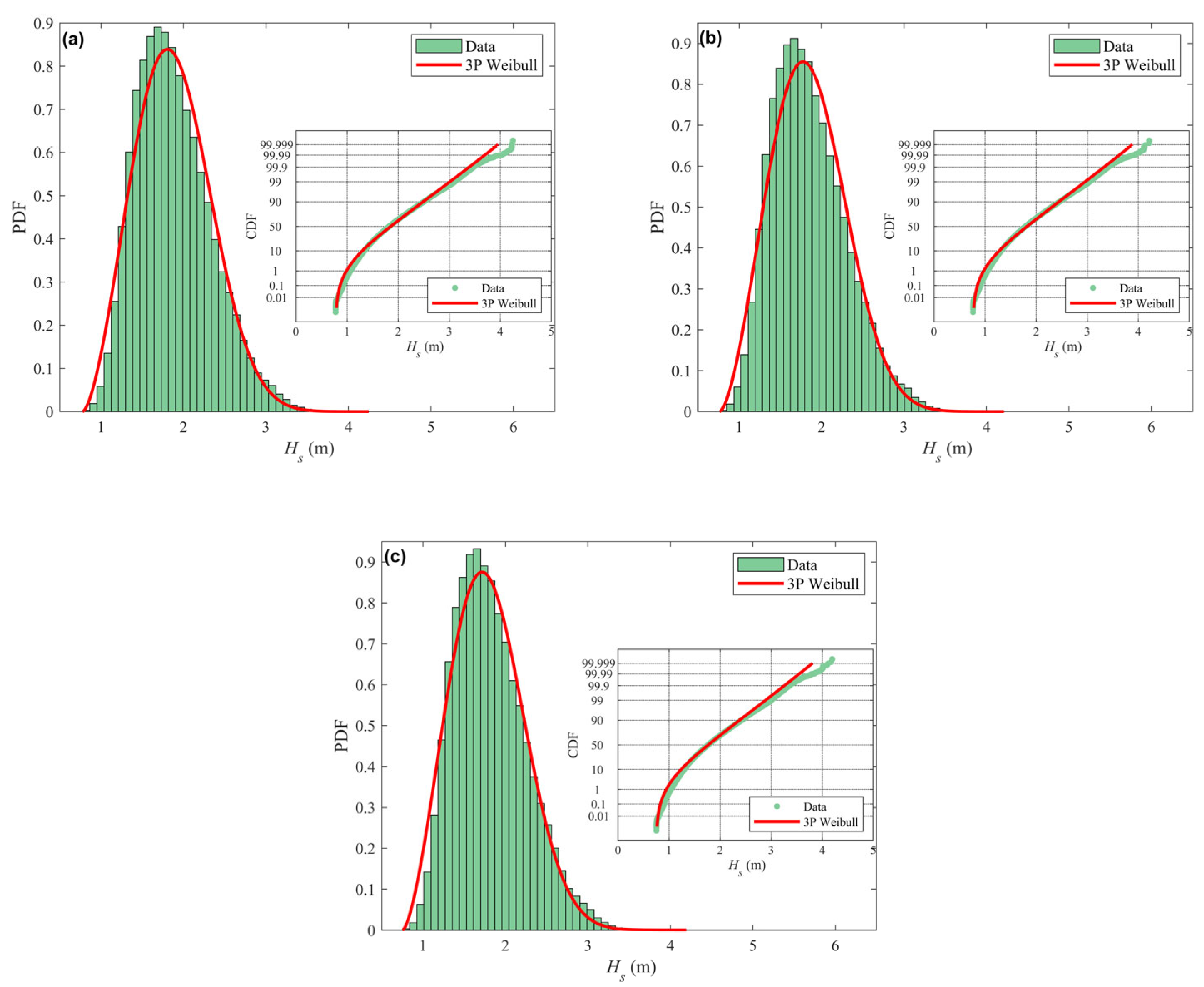
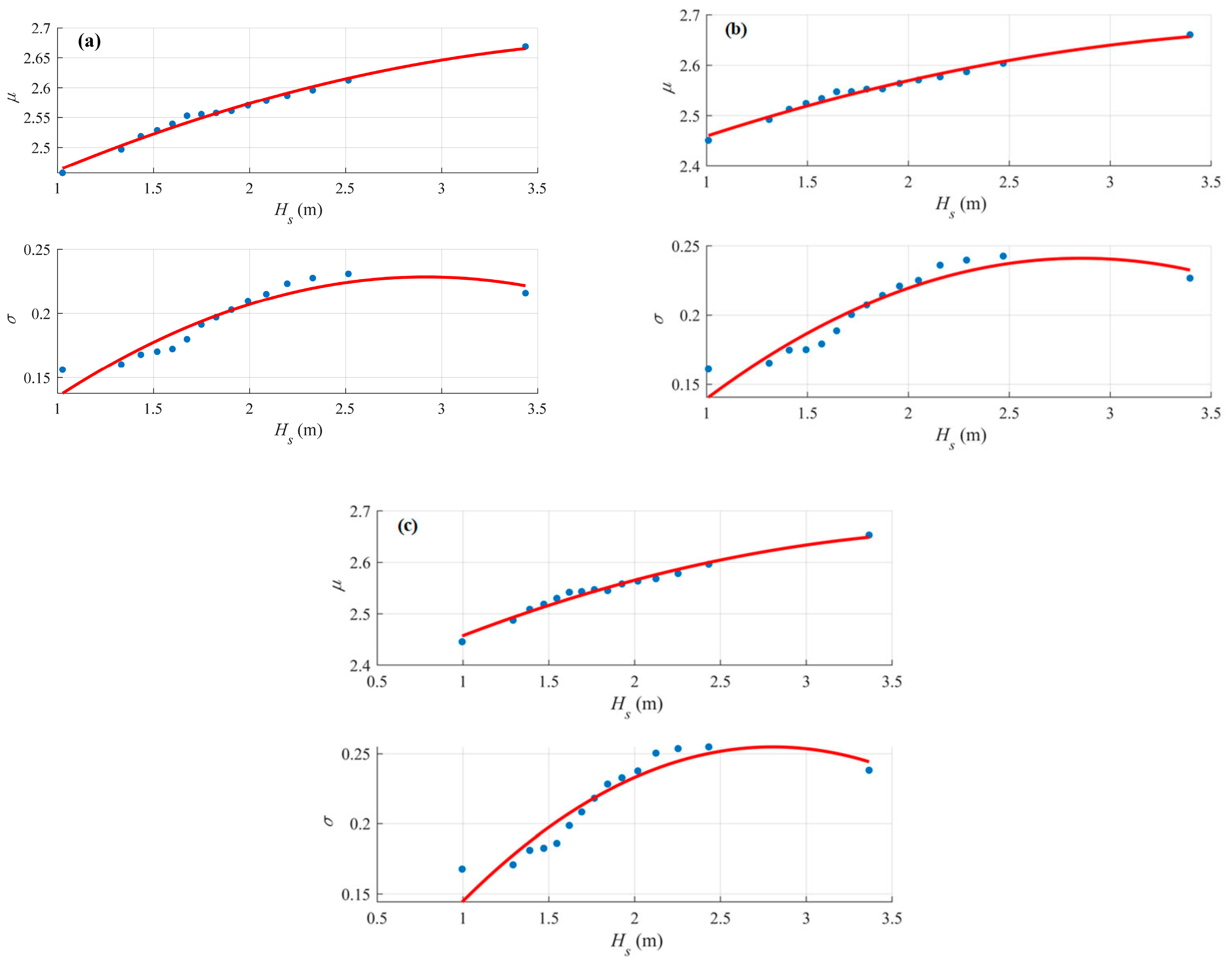
DatasetModelKSKS0.05χ2T χ 0.95 2
13-P Weibull0.0255(F)0.00264.66 × 103(F)815.51
Gaussian mixture0.00100.002613.63916.92
23-P Weibull0.0272(F)0.00264.87 × 103(F)815.51
Gaussian mixture0.00150.002616.31916.92
33-P Weibull0.0332(F)0.00265.71 × 103(F)815.51
Gaussian mixture0.00110.002613.65916.92
Table 14. Predicted design sea states derived from conditional Weibull–Lognormal and Gaussian mixture contours for wave simulations at three locations.
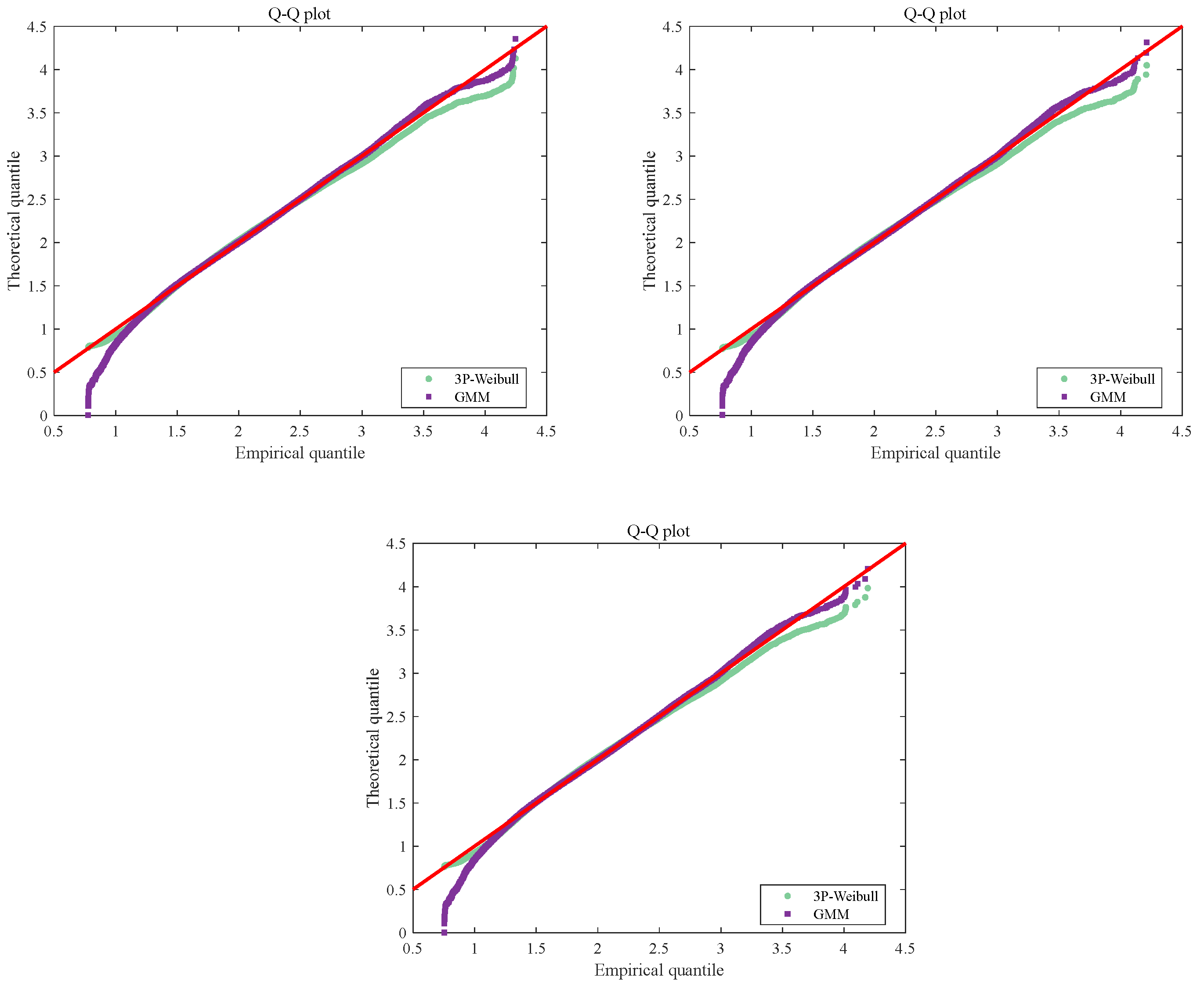
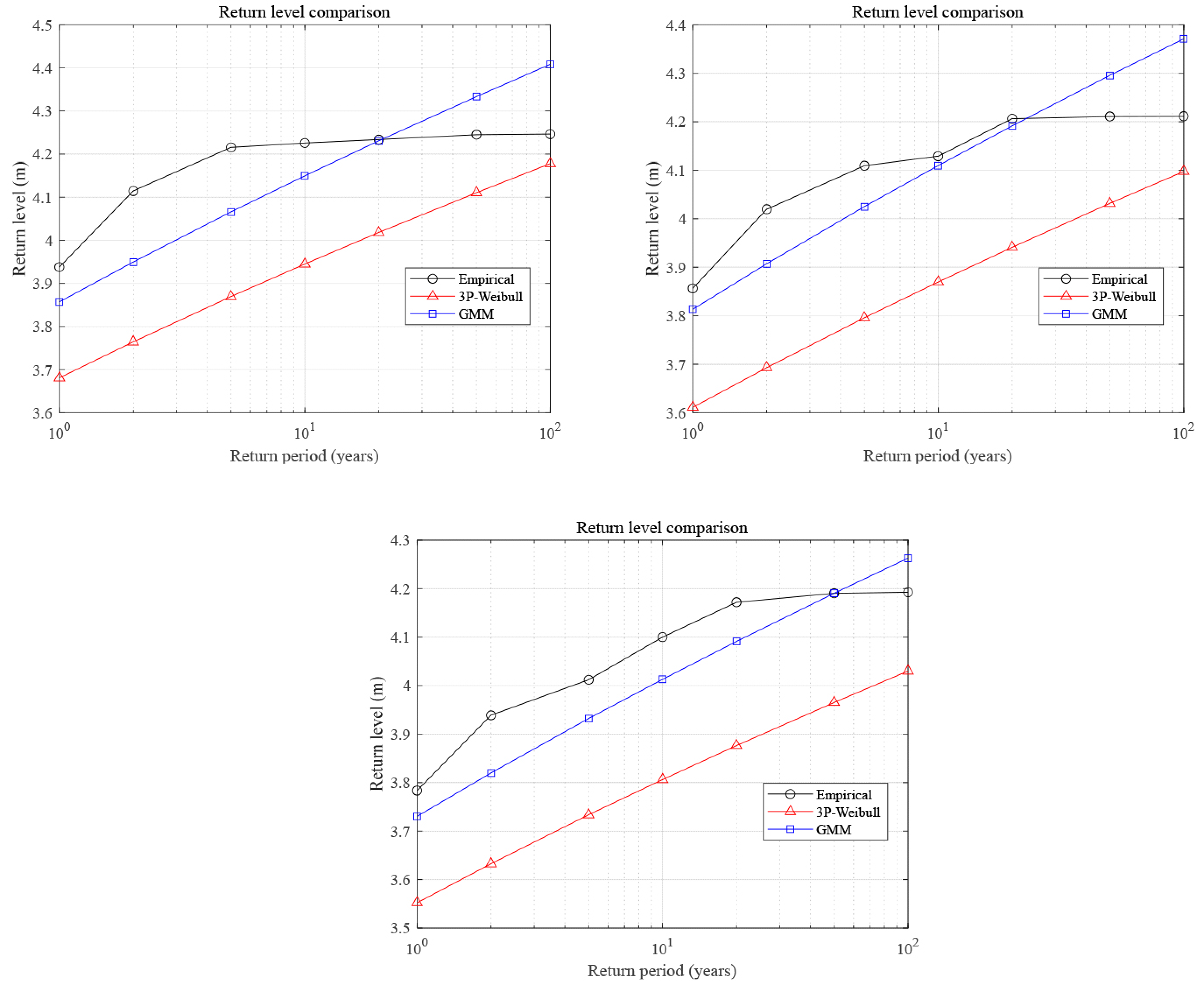
DatasetReturn PeriodModelMaximum Hs (m)Associated Tp (s)Maximum Tp (s)Associated Hs (m)
15-yearWeibull–Lognormal3.8714.5432.472.50
Gaussian Mixture4.1918.4022.811.60
100-yearWeibull–Lognormal4.1814.6037.882.57
Gaussian Mixture4.5518.8024.131.50
25-yearWeibull–Lognormal3.8014.4133.772.45
Gaussian Mixture4.1319.2022.881.70
100-yearWeibull–Lognormal4.1014.4639.732.53
Gaussian Mixture4.4820.3024.201.70
35-yearWeibull–Lognormal3.7214.2835.122.41
Gaussian Mixture3.9518.3022.621.60
100-yearWeibull–Lognormal4.0214.3441.702.46
Gaussian Mixture4.1918.9023.941.50
Disclaimer/Publisher’s Note: The statements, opinions and data contained in all publications are solely those of the individual author(s) and contributor(s) and not of MDPI and/or the editor(s). MDPI and/or the editor(s) disclaim responsibility for any injury to people or property resulting from any ideas, methods, instructions or products referred to in the content.