Article

Comparative Studies of Physics- and Machine Learning-Based Wave Buoy Analogy Models Under Various Ship Operating Conditions

HD Hyundai Heavy Industries Co., Ltd., Seongnam 13553, Republic of Korea
*
Author to whom correspondence should be addressed.
J. Mar. Sci. Eng. 2025, 13(9), 1823; https://doi.org/10.3390/jmse13091823
Submission received: 1 September 2025 / Revised: 16 September 2025 / Accepted: 18 September 2025 / Published: 20 September 2025
(This article belongs to the Special Issue Machine Learning for Prediction of Ship Motion)

Abstract

This study presents a comparative analysis of wave buoy analogy models for sea state estimation. A nonparametric, response amplitude operator-based model is introduced as a physics-based approach, while a convolutional neural network is adopted as a machine learning approach. Using time-domain simulation data of wave-induced ship motions under various operating conditions, the accuracy and reliability of each model’s estimation are evaluated. The sensitivity of the physics-based model to operating conditions is examined, along with optimization strategies such as hyperparameter tuning. In particular, regularization techniques based on bilinear and B-spline surface fitting are applied to the nonparametric model, and the effects of interpolation techniques on model performance are assessed. For the machine learning model, a parametric study is conducted to determine input data types and formats, including time series and spectral representations, as well as the required length of the time window and dataset volume. Finally, the feasibility of the proposed neural network in estimating not only sea state parameters but also loading and navigational information, such as ship speed and GM, is discussed.

1. Introduction

In recent years, advances in computing power and digital technologies have led to growing interest in the development of operational solutions for ships in real seaways. To meet this demand, the concept of the digital twin has been introduced at the operational phase as a platform for real-time fusion, processing, and analysis of sensor data, as well as for continuous information exchange between the physical ship and its virtual counterpart via performance monitoring and simulation [1,2,3]. In implementing a digital twin system, modeling the virtual ocean environment is as critical as constructing its virtual asset in cyberspace. In other words, the measurement and estimation of sea states around the vessel constitute core technologies for developing decision-support solutions for ship operators. Real-time sea state estimates can be utilized to monitor excessive ship motions and hull stresses and, further, provide operational safety guidance to mitigate risks such as cargo loss and capsizing. In addition, a database of encountered sea states during actual operations can be leveraged to evaluate speed-power performance and fuel consumption, considering added resistance induced by the ocean environment. Such performance assessments can provide feedback on hull form and on various energy-saving devices (ESDs), thereby enabling ship designs that reflect operational profiles (OPs) in real seaways.
In general, large commercial ships operate according to mid- and long-term voyage plans that incorporate weather forecasts, while responding to changes in the ocean environment during navigation based on the operator’s visual observations and empirical knowledge. However, weather forecast data inherently contains uncertainties in estimating sea states at the vessel’s exact location due to their coarse spatial resolution (typically 0.5 degrees latitude/longitude grids, approximately 50 km) and long update intervals (every 3 to 6 h). These uncertainties hinder the development of decision-support systems and the effective analysis of ship operation data. Therefore, to ensure the accuracy and reliability of operational solutions, real-time onboard wave measurements around the vessel are necessary. Marine radar technology [4,5,6], a representative method of onboard measurement, enables observation of the spatiotemporal evolution of the sea surface and the derivation of sea state information through post-processing. Nevertheless, marine radars have limitations, including high installation costs and a requirement for specialized expertise in calibration and maintenance. As an alternative, the wave buoy analogy (WBA) method, which estimates sea states from ship motion responses, provides a cost-effective solution requiring only relatively simple equipment such as a motion reference unit (MRU).
The wave buoy analogy (WBA), which has been continuously developed and applied over the past 20 to 30 years for sea state estimation, is fundamentally based on the relationship between ship motion dynamics and ocean waves in the frequency domain. Specifically, it involves an optimization process that minimizes the discrepancy between motion spectra obtained from measured time series data and those derived using response amplitude operators (RAOs) combined with an estimated wave spectrum. Frequency-domain WBA methods can be broadly categorized into parametric and nonparametric models. Parametric models [7,8,9,10,11,12] employ the parameterized forms of frequency spectrum and directional spreading function, offering advantages such as ease of interpreting sea states and avoidance of nonphysical optimization failures. However, they require significant computational resources for nonlinear optimization and may be prone to estimation errors due to convergence to local optima. In contrast, nonparametric models [13,14,15,16,17,18] are based on an unprescribed two-dimensional directional spectrum, providing greater flexibility and more degrees of freedom that can adapt to arbitrary wave energy distributions. Moreover, external estimation sources (e.g., marine radar measurements or machine learning models) can be incorporated through additional constraints, enabling integration with complementary methods [19]. However, to prevent overfitting of the numerical solution, regularization based on prior information about the geometric properties of the wave spectrum is required. As a result, sea state estimation results may be sensitive to the hyperparameters that determine the degree of regularization [20,21]. Further details on the theory and application of WBA are provided by [22,23].
The physics-based WBA models, which are indirect approaches rather than direct wave measurements, exhibit several limitations. First, optimization is constrained by the physical characteristics of wave-induced ship motions. Large commercial vessels act as low-pass filters, as they are not significantly excited by short waves (i.e., when the wavelength-to-ship-length ratio is below 0.5), which makes it difficult to capture high-frequency components. Furthermore, for a ship with forward speed in following or stern-quartering seas, the absolute and encounter frequencies exhibit a 1-to-3 relationship due to the Doppler effect, leading to motion responses concentrated within a narrow, low-frequency band. Consequently, to estimate the wave spectrum in terms of absolute frequencies, the motion energy at encounter frequencies must be accurately redistributed in reverse to reflect the original wave energy distribution. This inverse process may cause optimization failures, such as overfitting to high-frequency components [24,25]. Second, the physics-based model is rigidly dependent on RAOs. The motion transfer functions are generally computed using linear potential-flow methods, such as two-dimensional strip theory or three-dimensional panel methods. However, such seakeeping computations have limitations for addressing ship motions at high forward speeds or in large-amplitude waves, where significant nonlinear effects occur, resulting in discrepancies between theoretical models and actual ship dynamics. Moreover, operational data such as loading and navigational conditions contain inherent measurement uncertainties, which can propagate directly into errors in sea state estimation.
In recent years, machine learning (ML) models have been increasingly adopted within the WBA framework to overcome the limitations of physics-based approaches. These models can directly map the relationship between ocean environments and ship motions without relying on RAOs, even under uncertainties in loading and navigational conditions. In data-driven approaches, when sufficiently large datasets are available, accurate sea state estimation can be achieved even from the limited information contained in measured motion data, which is often distorted by the ship’s filtering effects. Within the WBA, convolutional neural networks (CNNs) and long short-term memory (LSTM) networks are widely employed to identify patterns in motion responses [26,27]. More advanced CNN-based architectures, such as ResNet and Inception [28], as well as attention mechanisms [29], have also been employed in recent studies. Various models have been developed for different output variables, including sea state classification [30,31], regression of integrated sea state parameters, and estimation of the full directional wave spectrum [32,33]. Comparative studies on input-output data types and formats, as well as on different ML architectures, can be found in [34,35].
One of the most critical challenges highlighted in previous studies on the application of ML models is acquiring labeled datasets for supervised learning and the associated limitations in generalization across a wide range of sea states and ship operating conditions. In particular, many studies have reported a significant decline in estimation accuracy in rare events, such as extreme sea states. To address this limitation, it is essential to perform uncertainty analyses of model inference and to improve model generalization by integrating physics-based models or leveraging transfer learning with numerical simulation data [36,37,38].
In this study, a comparative analysis is conducted between WBA models for sea-state estimation. A nonparametric, RAO-based model is adopted as the physics-based approach, while a CNN architecture is employed as the machine learning model. Time-domain numerical simulations are performed to generate synthetic ship-motion time series under various sea states and operating conditions, which is subsequently used for model validation and performance assessment. For the physics-based model, bi-linear and B-spline surface interpolation and regularization techniques are incorporated to optimize the numerical solution, and the resulting accuracy and reliability are evaluated across different operating conditions. For the machine learning model, a parametric study is carried out on the input–output data configurations to examine the optimal data types and formats. Finally, the applicability of the ML model is discussed not only for sea state estimation but also for the inference of ship loading and navigational information.

2. Theoretical Backgrounds

2.1. Problem Definition

This study considers a ship operating in an ocean environment characterized by irregular, short-crested random seas. For each wave component, χ and ω indicate the propagating direction and absolute frequency, and A and ε are its amplitude and phase, respectively. The ocean wave field is described in the Earth-fixed global coordinate system (O–XYZ) using a finite set of discretized wave components:
ζ X , Y , t = m n A m n e x p i k n X c o s χ m + k n Y s i n χ m ω n t + ε m n ,
where k is the wave number that satisfies the deep-water dispersion relation, ω2 = gk. The six degrees-of-freedom (DOF) wave-induced ship motions are defined with respect to the inertial coordinate system (o–xyz), which translates with the ship at a forward speed U. These motions consist of translational responses (surge ξ1, sway ξ2, and heave ξ3) and rotational responses (roll ξ4, pitch ξ5, and yaw ξ6). The relationship between the global and inertial coordinate systems is determined by the ship’s yaw angle (heading angle ψ). The coordinate systems and definitions are illustrated in Figure 1.
The present study is based on the following assumptions. First, the wave field is modeled as a Gaussian random process with stationary and homogeneous properties. Moreover, the wave height and the resulting ship motion responses are assumed to be small (kA, ξi ≪ 1) and are approximated as following a linear relationship. The ship is further considered to operate under steady-state navigational conditions, implying slow time variations in maneuvering. Accordingly, both the ship’s forward speed and heading angle are assumed constant, with the heading angle set to zero (ψ = 0).

2.2. Physics-Based Model: Nonparametric Model

In the physics-based model, ocean waves and ship motion responses are related in the frequency domain, such that:
S i j ω e = 0 2 π H i χ , ω e H j χ , ω e E χ , ω e d χ ,
where Sij denotes the cross spectra of the i-th and j-th motion mode time series. Similarly, Hi and Hi* represent the complex transfer function of the i-th motion mode and its conjugate, respectively. E is the directional wave spectrum, which serves as the solution to the governing equation. According to the relationship between the absolute frequency ω and encounter frequency ωe due to the Doppler effect, characterized by a 1-to-3 mapping, i.e., ωe = ω − αω2 where α = Ucosχ/g, the right-hand side of Equation (2) is transformed into the absolute-frequency domain and subsequently discretized with respect to wave directions, yielding:
S i j ω e = χ m = 1 M H i j m ω 1 E χ m , ω 1 d ω 1 d ω e                     + χ m = 1 M H i j m ω 2 E χ m , ω 2 d ω 2 d ω e                     + χ m = 1 M H i j m ω 3 E χ m , ω 3 d ω 3 d ω e where   H i j m ω a = H i χ m , ω a H j χ m , ω a .
Here, ωa for a = 1, 2, 3 denote the absolute frequencies for a given encounter frequency (see Figure 2). Among them, ω1, always exists, whereas ω2 and ω3 appear only under following or stern-quartering wave conditions, when cosχ > 0.
In this study, heave, roll, and pitch motions are selected as the response set. In particular, the roll response is selected as a port-starboard asymmetric mode to capture wave directionality. Accordingly, by the Hermitian property of the motion spectra, Sij = Sij*, where Sij = Cij + iQij, a total of nine spectra is employed to construct the governing equation. For the l-th encounter frequency ωe,l, the matrix equation is formulated as follows:
N l b l = N l A l F l f where   b l 9 × 1 = S 33 l S 44 l S 55 l C 34 l C 45 l C 53 l Q 34 l Q 45 l Q 53 l T , A l 9 × 3 M = χ H 33 m ω a H 44 m ω a H 55 m ω a R e H 34 m ω a R e H 45 m ω a R e H 53 m ω a I m H 34 m ω a I m H 45 m ω a I m H 53 m ω a d ω a / d ω e , f M N × 1 = E m n .
Here, Nl(9 × 9) is the normalization matrix to standardize the motion cross-spectral terms. According to [39], the real and imaginary parts of each component are independently normalized, such that
C i j l ^ = C i j l 1 2 S i i l S j j l + C i j l 2 Q i j l 2   ,   Q i j l ^ = Q i j l 1 2 S i i l S j j l C i j l 2 + Q i j l 2 .
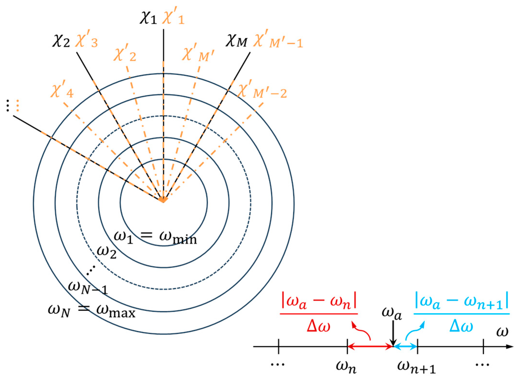
The solution f consists of a wave spectrum that is uniformly discretized into M directions and N absolute frequencies: Emn = E(χm, ωn), as shown in Figure 3. It should be noted that the discretized directions in the solution can be different from those used in the governing equation, i.e., M’ directions. In general, to incorporate more directional information, the wave spectrum is evaluated at a greater number of directions (M’ > M). Furthermore, the absolute frequencies corresponding to ωe,l, which are determined by the ship speed and wave direction, do not exactly coincide with the discretized frequencies of the solution. Therefore, an interpolation matrix Fl(3M’ × MN) is required to evaluate the wave spectrum at the governing equation’s collation points: fl(3M’ × 1) = [E(χ’m, ωa)].
Two interpolation methods are introduced. The first is a simple bilinear interpolation, which uses the solution values of the four nearest bins in direction and in absolute frequency. The second method employs B-spline surface interpolation. Based on the cubic B-spline basis function Bnp of order p = 3, the surface of the wave spectrum can be expressed as follows:
E χ , ω = m = 0 N c , χ 1 m = 0 N c , ω 1 c m n B m p u B n p v   ,
where u and v are the surface parameters obtained by normalizing the direction and frequency, respectively. cmn denotes the control points, and Nc,χ and Nc,ω are the numbers of control points along each axis. For cubic B-splines, Nc,χ = M + 2 and Nc,ω = N + 2. The B-spline basis function follows the Cox-de Boor recurrence formula, such that
B m p u = u u m 1 u m + p 1 u m 1 B m 1 p 1 u + u m + p u u m + p u m B m p 1 u where   B m 0 u = 1 w h e n   u m 1 u u m 0 e l s e ,   m = 0 N c 1 B m p u = 1 .
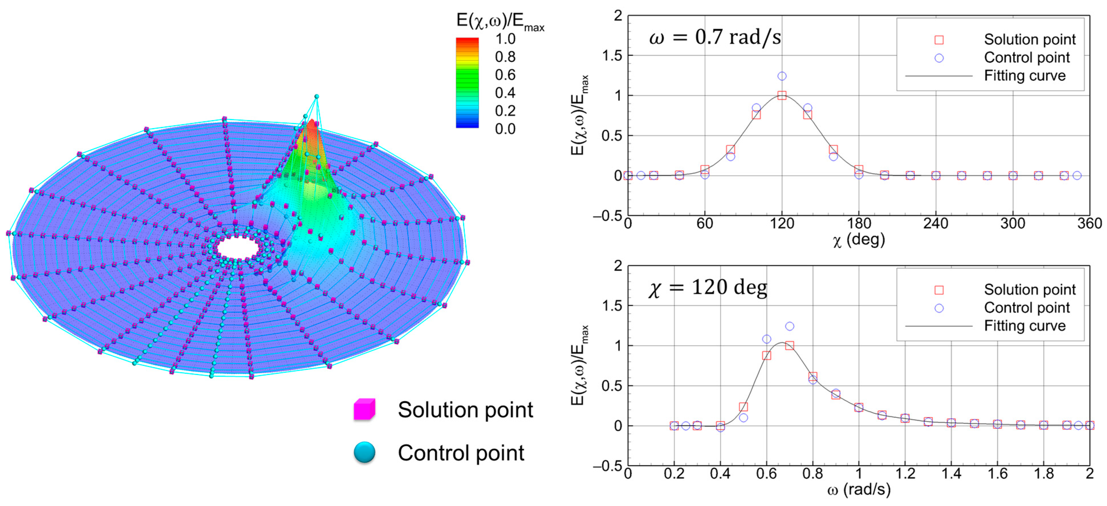
Here, um for m = 1, …, κ are the knots, where κ = Nc + 4. It should be noted that, by aligning the control points with the solution points and placing the remaining two between the solution points at both boundaries, additional boundary conditions are satisfied along each axis: circular boundary conditions along the direction axis (C0, C1, and C2 continuities) and zero-gradient conditions along the frequency axis (∂E/∂ω = 0), as shown in Figure 4. In summary, the B-spline surface interpolation can be expressed in matrix form as follows:
f l = B l χ m , ω a c where   c M N × 1 = D c f .
Here, Dc denotes the mapping matrix between the control points c and the solution vector f. In addition, Bl(χ’m, ωa) is the evaluation matrix composed of cubic B-spline basis functions, which is used to perform interpolation at the collocation points according to Equation (6).
For a given set of encounter frequencies defined in spectral analysis (a total of L encounter frequencies), the governing equation can be formulated to serve as the basis for data fitting. However, the numerical solution may be susceptible to overfitting due to noise and biases in the motion measurements, uncertainties in the ship operation data, and numerical errors in RAO computations. Therefore, regularization based on prior information about the wave spectrum is required to stabilize the solution. The most representative prior assumption is that the wave spectrum exhibits continuity and smoothness, often referred to as a smoothness constraint. The implementation of this constraint varies depending on the interpolation method. For bilinear interpolation, it is commonly assumed that the second-order derivatives vanish to prevent locally abrupt variations in the wave spectrum. By introducing finite differences, the regularization equation is formulated as follows:
β χ D χ β ω D ω f = 0 where   D χ f = E m 1 n 2 E m n + E m + 1 n ,   D ω f = E m n 1 2 E m n + E m n + 1
Here, Dχ and Dω denote the regularization matrices representing the second-order derivatives along each axis, and βχ and βω are hyperparameter matrices that specify the strength of regularization at the discretized solution points. A detailed explanation of the regularization matrices based on bilinear interpolation can be found in [14]. Alternatively, in B-spline surface interpolation, the smoothness constraint is imposed by penalizing discrepancies between the control points and the solution values. Specifically, a regularization equation is formulated to minimize distances between them:
β s D s f = 0 where   D s = D c I .
For bilinear interpolation-based regularization, constraints are applied independently along the direction and frequency axes, using only four adjacent solution points. In contrast, B-spline surface-based interpolation and regularization provide more accurate data fitting through higher-order basis functions and enable two-dimensional surface-based constraints that use sixteen adjacent solution points. More comprehensive descriptions of higher-order surface-based regularization can be found in [40,41].
Finally, the complete system equations of the physics-based model, incorporating both the governing equations and the regularization terms, are formulated as follows:
min f > 0 N A F f N b 2 + β D f 2 .
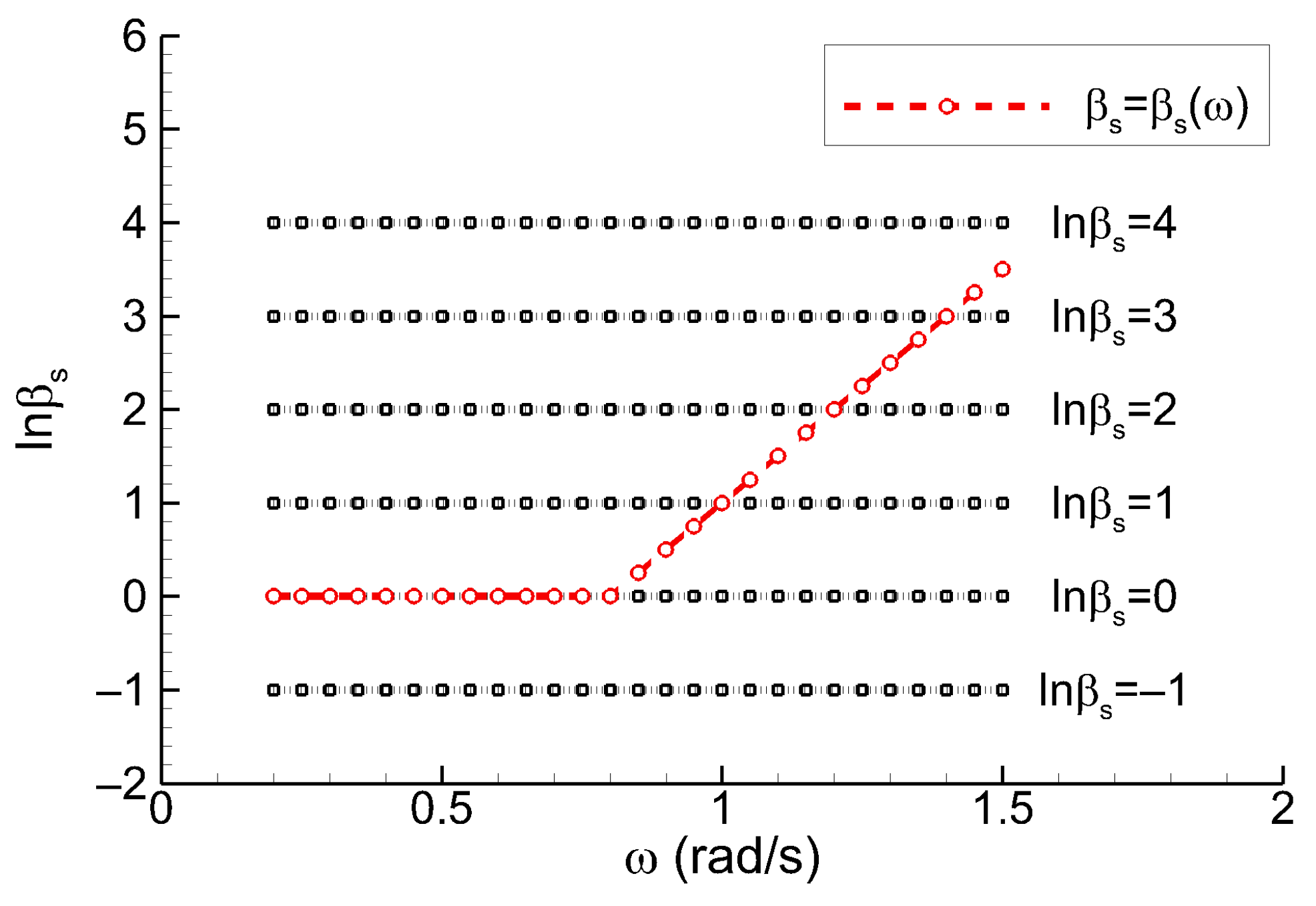
To obtain the numerical solution, the non-negative least-squares (NNLS) method is employed. Table 1 summarizes the computational parameters used to construct the physics-based model. These parameters are determined by considering typical sea states, ship operating conditions, and the resulting ranges of motion responses. A key issue in the solution procedure is the selection of an optimal hyperparameter, which balances the governing equations (data fitting) and the regularization terms (stabilizing functionals). The hyperparameter can be assigned as a constant value across the entire solution domain or defined as a frequency-dependent function specified for particular intervals. To account for arbitrary wave directions, the hyperparameter is not defined as a function of direction. In this study, for the B-spline method, the following piecewise function is adopted, in which the degree of regularization increases with frequency, as illustrated in Figure 5:
β s ω = 1 w h e n   ω < 0.8   r a d / s e x p 5 ω 4 w h e n   ω 0.8   r a d / s

2.3. Machine Learning Model

Ship motions induced by waves depend not only on ocean environments, such as wave height, period, and direction, but also on the ship’s loading and navigational conditions. By employing machine learning models, it is possible to discover patterns from historical motion data and directly map them to sea state information in an end-to-end manner, without defining the equations of motion and solving hydrodynamic boundary value problems, that is, without relying on motion RAOs. In particular, when a sufficiently large and high-quality dataset is available for supervised learning, statistically convergent data-driven models can be constructed, which account for inherent uncertainties in measured ship operation data. Moreover, an artificial neural network (ANN) architecture comprising input, hidden, and output layers with affine functions (i.e., continuous weighted sums and biases) and nonlinear activation functions, can capture complex nonlinear ship motion dynamics, such as large-amplitude wave-induced responses and viscous damping effects on resonant roll motions, in accordance with the universal approximation theorem. Lastly, while physical models require prior loading and navigational information such as draft, center of gravity, radius of gyration, and ship speed, machine learning models can inversely infer the underlying operating conditions from motion responses: an inverse operator.
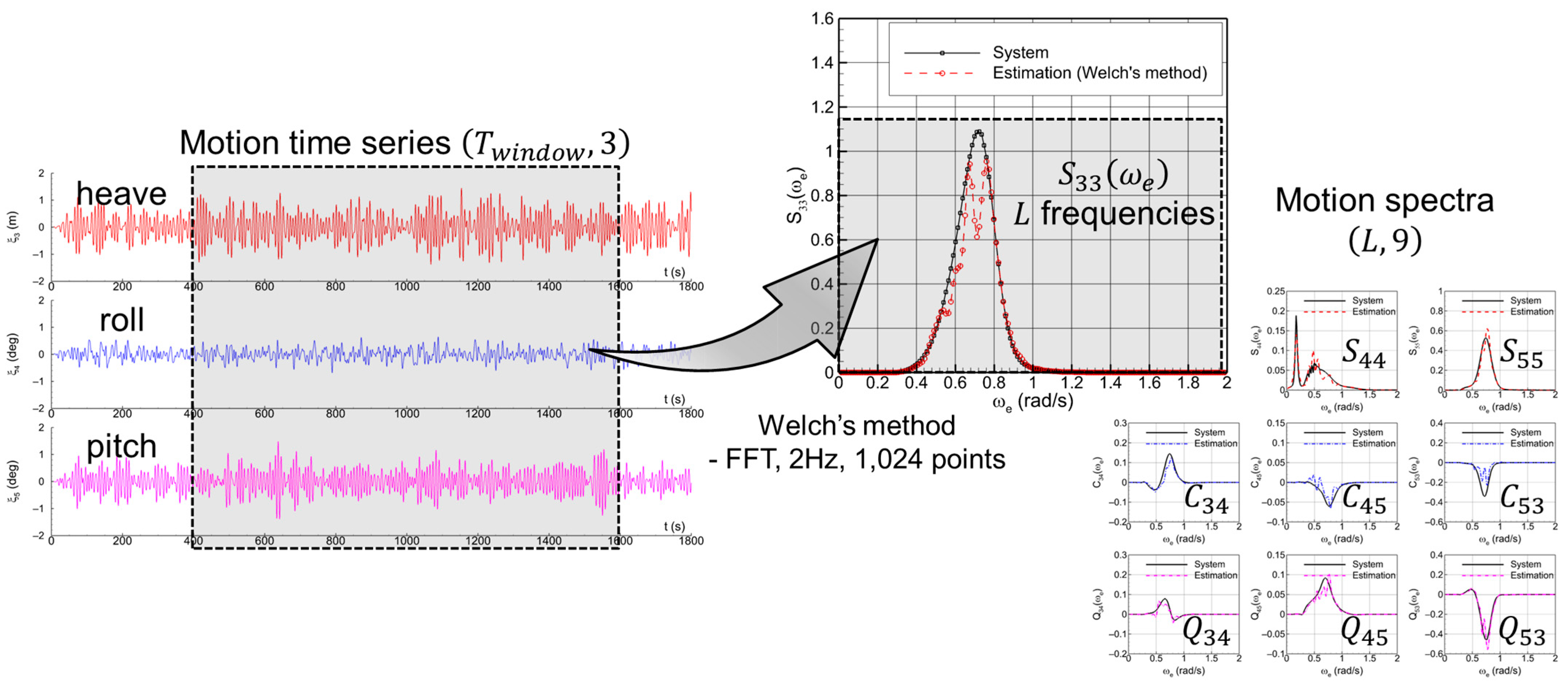
In the present study, a multivariate regression model is developed to estimate sea states and ship operation information from motion response data. Two types of input data are considered: (1) time series data (2) cross-spectral data (see Figure 6). The time-domain input consists of three DOF responses (heave, roll, and pitch) as in the physics-based model. These raw time series data naturally contain phase difference information between responses, which is essential for capturing wave directionalities. The sampling frequency is set to 2 Hz, and the machine learning model is trained and evaluated over various time windows Twindow ranging from 5 to 30 min. Accordingly, the dimension of the time-domain input data is (600~3600, 3). In the frequency domain, input data are composed of cross spectra for pairs of motion signals, which also contain the phase relationships. For the three DOF responses, a total of nine spectral components is utilized: three auto spectra and six cross spectra (real and imaginary parts of three coupling terms). The Fourier transform-based spectral analysis is performed using Welch’s method on 1024-point time series data comprising 256-s motion data and 256-s zero-padded data. From the resulting spectra, uniformly spaced components are extracted based on the specified number (L) and resolution (Δωe) of encounter frequencies. As a result, the dimension of the frequency-domain input data is (L, 9).
The output variables consist of sea state parameters and ship operating conditions. The sea state parameters are defined by integration over the directional wave spectrum. In this study, the significant wave height HS, the zero up-crossing mean period T2, and the main wave direction χM are selected as the representative parameters:
H S = 4 m 0 ,   T 2 = 2 π m 0 / m 2 ,   χ M = t a n 1 d 1 ω d ω / c 1 ω d ω where   S ζ ω = E χ , ω d χ ,   m n = ω n S ζ ω d ω , c 1 ω + i d 1 ω = e x p i χ E χ , ω d χ .
Here, Sζ(ω) and mn denote the wave frequency spectrum and the n-th-order spectral moment, respectively. c1(ω) and d1(ω) are the first-order directional Fourier coefficients. In addition, two operational variables, speed through water STW and metacentric height GM, which represent the ship’s navigational and loading conditions, are also included as output features. Because such operational parameters significantly influence the vessel’s seakeeping performance while varying slowly over time, that is, serving as tagging information with low variance, they are treated as output variables rather than inputs. This approach is expected to improve the accuracy of sea state estimation, as suggested by [28]. Moreover, this study investigates whether the machine learning model can capture the underlying operational variables implicitly embedded in the ship motion responses. In total, the ML model is developed to predict six output variables (multioutput regression): (HS, T2, cosχM, sinχM, STW, GM).
Compared with conventional machine learning models, deep-learning architectures are inherently more scalable to high-dimensional and large-volume datasets, enabling the extraction of underlying data structures and exhibiting superior predictive accuracy and generalization capability. Among various deep learning models, convolutional neural networks (CNNs) are particularly effective in processing continuous spatiotemporal data and have been widely adopted in diverse applications such as image segmentation and object detection. CNNs are also applicable to multivariate time series and spectral data for identifying distinctive patterns and subsequently performing regression on target variables.
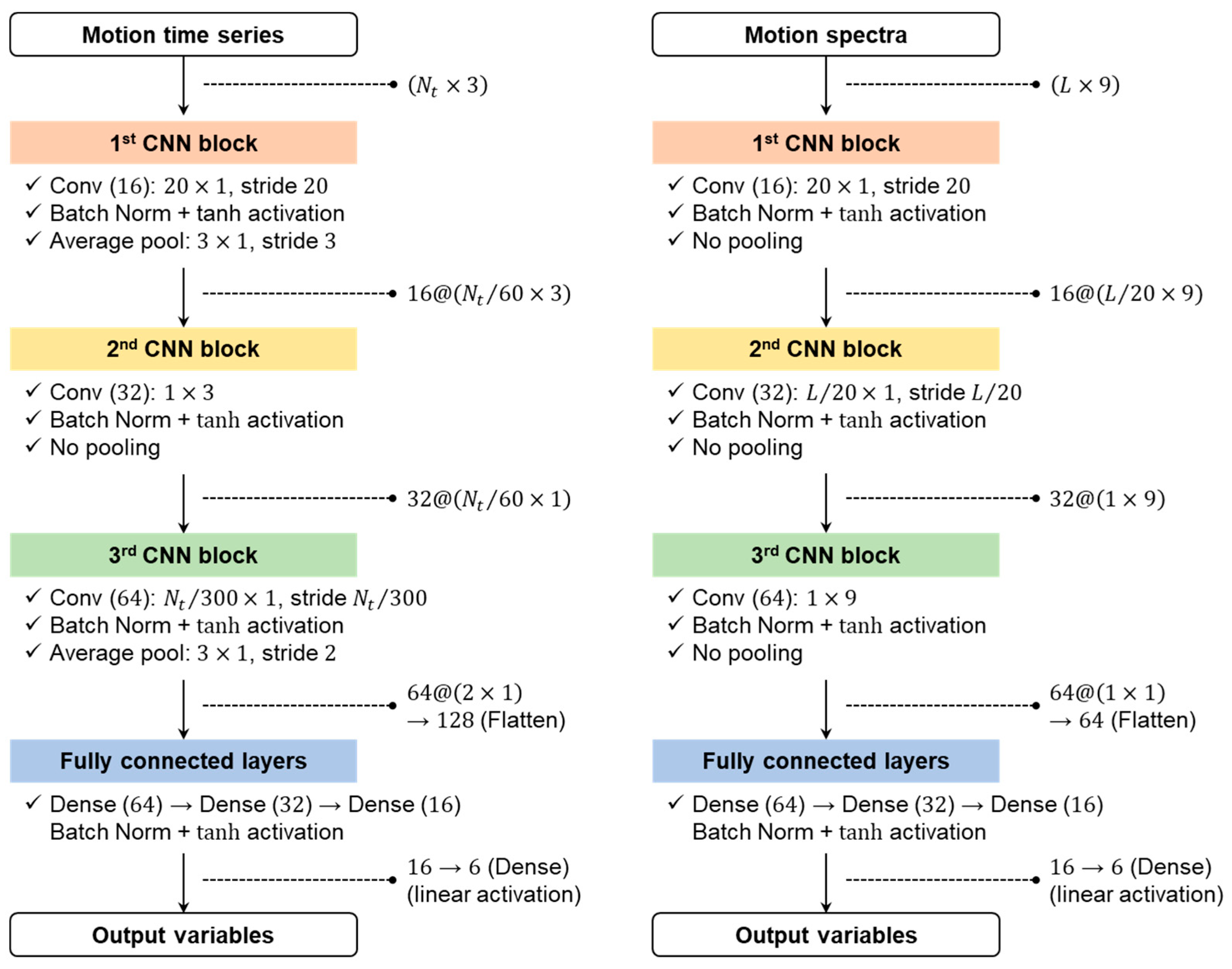
The proposed model architecture consists of multiple sequential CNN blocks that progressively encode hierarchical features from the input to the output. The CNN architecture includes one block that applies one-dimensional convolution along the time or frequency axis, as well as another block that applies one-dimensional convolution across response variables to capture inter-response correlations, such as phase differences. Each CNN block comprises the following components: (1) convolution, (2) batch normalization, (3) nonlinear activation, and (4) average pooling. In the convolution process, shared weights, referred to as kernels or filters are employed to extract local features from receptive fields while simultaneously identifying global dependencies among different parts. The filter parameters are invariant to temporal or spatial positions to generalize the system: a parameter sharing. In this study, the filter size and stride are identically set to reinforce the spatiotemporal invariance. During convolution, the data undergo lossy compression, i.e., downsampling, effectively eliminating redundant information. To mitigate overfitting, L2 regularization with a penalty coefficient of 0.001 is applied to the filter parameters. Batch normalization is performed prior to the activation function to stabilize the training process and reduce sensitivity to hyperparameter configurations. Finally, average pooling is used to smooth the feature representations and further promote generalization performance. The output of the CNN blocks is fed into three fully connected layers to interpret the encoded latent features, with the final layer using a linear activation function to perform regression. The model architecture is consistent for both time-domain and frequency-domain inputs, and the detailed structures are illustrated in Figure 7.
Beyond the CNN-based regression model adopted in the present study, various machine learning models, such as advanced CNN architectures (e.g., ResNet and Inception) and sequence-processing networks (e.g., multivariate LSTM and attention-based models), can also be applied to sea state estimation using ship motion responses. Comparative studies of different ML models have been extensively conducted [28,34,35], and recent research [29] has shown that when each model’s architecture (i.e., the number of layers, neurons, and filters) is optimized, their performance becomes similar. In particular, the CNN-based regression model and the attention-based network have been found to produce results of comparable accuracy. Therefore, it should be noted that this study focuses not on the comparison of ML models, but rather on the performance evaluation and validation between the CNN-based model and the physics-based model.
The present machine learning models are implemented using the Keras Functional API and trained via backpropagation with stochastic gradient descent (SGD). Model parameters are optimized by minimizing the mean squared error (MSE) loss function using the adaptive moment estimation (Adam) optimizer, with hyperparameters β1 = 0.9 and β2 = 0.999. Training is performed for 5000 epochs with a batch size of 128. The learning rate is initially set to 10−3 and progressively reduced to 10−5 during training based on the validation loss.

3. Analysis Results

3.1. Database and Test Conditions

In this study, numerical simulations have been conducted for the well-known KCS containership to construct a synthetic ship motion database. The principal dimensions of the ship model are summarized in Table 2. For time-domain seakeeping computations, the impulse response function (IRF) method is employed. In the IRF method [42], the six DOF equations of ship motions are defined as follows:
M i j + M i j ξ ¨ j + t R i j t τ ξ ˙ j τ d τ + C i j + C i j R ξ j = F e x t , j .
Here, M and M denote the mass matrix and the infinite-frequency added mass, respectively. Moreover, the terms C and CR indicate the hydrostatic and radiation restoring coefficients. The retardation function R(t), appearing in the convolution integral, represents the memory effects of wave-induced motion and is related to the frequency-dependent added mass A(ω) and damping coefficient B(ω) as follows:
R i j t = π 2 0 B i j ω c o s ω t d ω ,
M i j C i j R ω 2 = A i j ω + 1 ω 0 R i j τ s i n ω τ d τ .
The frequency-domain solutions including the hydrodynamic coefficients and the wave excitation force Fext(χ,ω), which are required for time-domain conversion, are computed by means of the two-dimensional strip theory [43]. Although more sophisticated methods of seakeeping analysis, such as the three-dimensional panel method or computational fluid dynamics (CFD), could be employed to calculate hydrodynamic forces, this study focuses on evaluating the performance of sea state estimation of both physics- and machine learning-based wave buoy analogy models. Therefore, the slender-body theory, which enables efficient database construction, is adopted.
Synthetic ship motion time series were generated over a wide range of sea states and operating conditions. Table 3 summarizes the test conditions adopted for database construction. Regarding loading conditions, the draft is fixed at its design value, while GM is varied from 0.5 m to 4.5 m by adjusting the ship’s vertical center of gravity. In addition, considering typical containership operations and voluntary speed reductions in severe sea states, the ship speed (STW) is assumed to range from 5 knots to 21–(gHS)1/2 knots. With respect to the ocean environment, a unimodal short-crested wave field is modeled. The sea states are characterized by significant wave heights ranging from 1 m to 6 m and peak periods determined by the empirical relation: Tp/(HS)1/2 = 4.5~5.5, with waves assumed to be incident from all directions, i.e., a main wave direction ranging from 0 degrees to 360 degrees. The frequency spectrum and directional spreading function used for modeling the synthetic ocean environment are defined as follows:
E χ , ω = D χ S ζ ω ,
S ζ ω = α γ 5 16 H S 2 ω p 4 ω 5 e x p 5 4 ω p ω 4 γ e x p ω ω p 2 2 σ f 2 ω p 2 where   α γ = 1 0.287 l n γ ,   σ f = 0.07 i f   ω ω p 0.09 i f   ω > ω p ,
D χ = 2 2 s 1 Γ 2 s + 1 π Γ 2 s + 1 c o s 2 s χ χ M 2 where   s = ω ω p 5 s m a x i f   ω ω p ω ω p 2.5 s m a x i f   ω > ω p .
Here, ωp = 2π/Tp is the peak spectral energy frequency. The peak enhancement factor γ determines the spectral shape, i.e., the bandwidth and is set to range from 1.0 (Pierson-Moskowitz spectrum) to 3.3 (JONSWAP spectrum). In addition, the spreading parameter s is defined as a function of the wave frequency, with smax ranging from 10 (wind waves) to 25 (swell with a short decay distance).
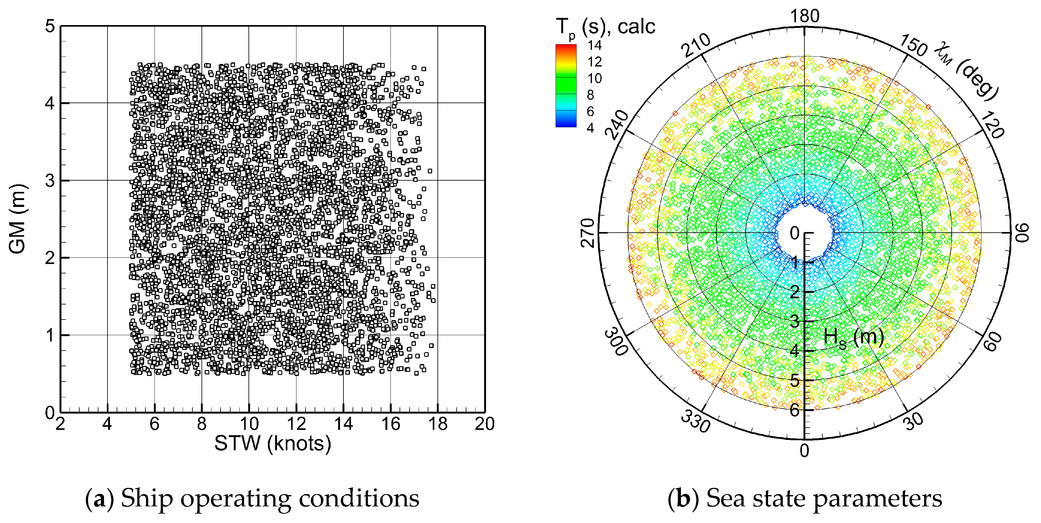
Based on the specified ranges of test conditions, ship operating conditions and sea state parameters for applying the WBA models were randomly sampled using Latin Hypercube Sampling (LHS). Figure 8 illustrates the 10,000 samples generated for training the machine learning models. An additional 1000 samples within the same ranges were prepared to evaluate the performance of both the physics-based and machine learning models. For each test condition, time-domain seakeeping simulation were performed. The incident wave components are defined by discretizing the directional wave spectrum into 300 frequency bins and 36 directional bins (at 10-degree intervals), yielding a total of 10,800 components. These components are then used to generate 30-min synthetic ship motion time series. To prevent repetition of motion responses, the discretized frequency intervals and component phases are randomly assigned for each seakeeping computation.
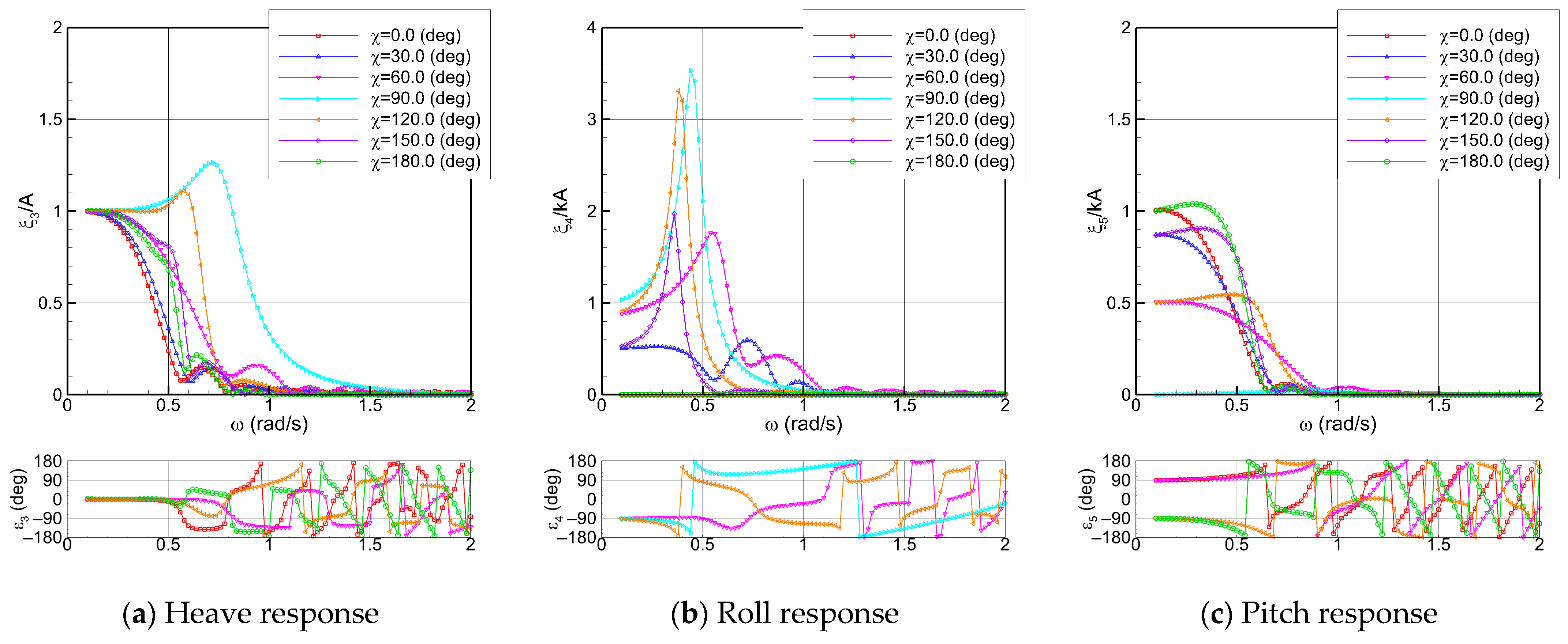
Lastly, a seakeeping database was established for the application of the physics-based model. The database specifications are summarized in Table 4. Consistent with the numerical simulations, the database of hydrodynamic coefficients and wave excitation forces was computed using the two-dimensional strip theory. By incorporating ship operating conditions from specific test data, such as GM and STW, the hydrodynamic coefficients are interpolated, and the mass and restoring matrices are constructed. These matrices are then used to set up the frequency-domain equations of motion, which are solved to obtain the motion transfer functions as shown in Figure 9. Due to the interpolation process, the derived RAOs may slightly deviate from the ship’s actual hydrodynamic characteristics used to generate synthetic motion time series. During real-time operation of the WBA models, uncertainties in loading conditions and navigational data inevitably exist. Therefore, the resulting discrepancies can be regarded as a realistic reflection of such uncertainties, given that the use of perfectly accurate RAOs is inherently infeasible.

3.2. Results of Physics-Based Model

Across the 1000 test samples, the physics-based models incorporating two interpolation and regularization schemes are applied to evaluate and compare the sea state estimation results. As shown in Figure 10 and Figure 11, the trends in the results with respect to the hyperparameters governing the smoothness constraints are similar for both the bilinear and B-spline methods. As regularization intensifies, the significant wave height, which represents the total wave energy, tends to be underestimated due to the smoothing effect. In contrast, the mean period, which reflects the energy distribution, slightly increases when high-frequency overfitting is mitigated. Regarding the main wave direction, regularization suppresses nonphysical components aligned with incorrect propagation directions, thereby leading to more stable estimates. Figure 12 illustrates the frequency spectrum and directional spreading function for a representative test case, obtained by integrating the two-dimensional directional spectrum along each axis. The effects of regularization on the spectrum are evident, and the reconstructed spectrum closely matches the exact solution when an appropriate hyperparameter value is adopted.
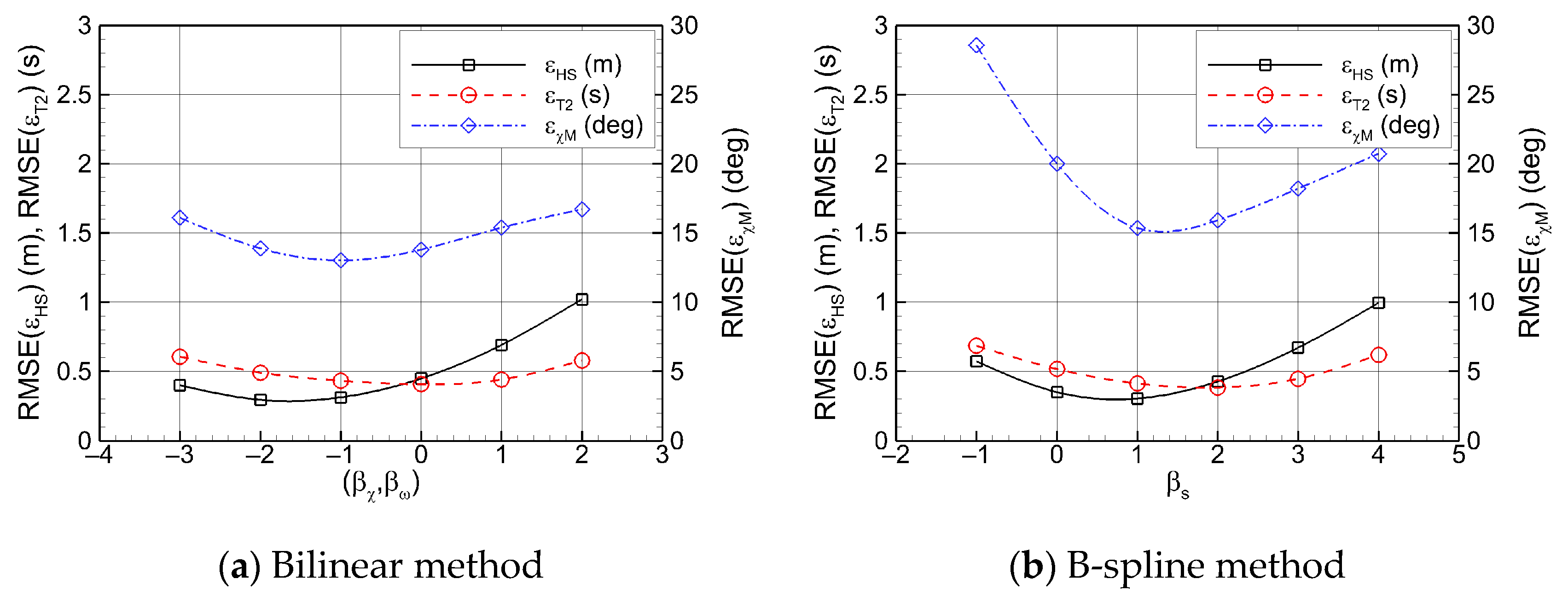
Figure 13 presents the root mean squared error (RMSE) of sea state parameters x ∈ [HS, T2, χM] to evaluate the performance of the physics-based model across the entire test dataset.
R M S E x = 1 N d a t a n = 1 N d a t a ϵ x , n 2 , where   ϵ x , n = x e s t i m a t i o n , n x e x a c t , n
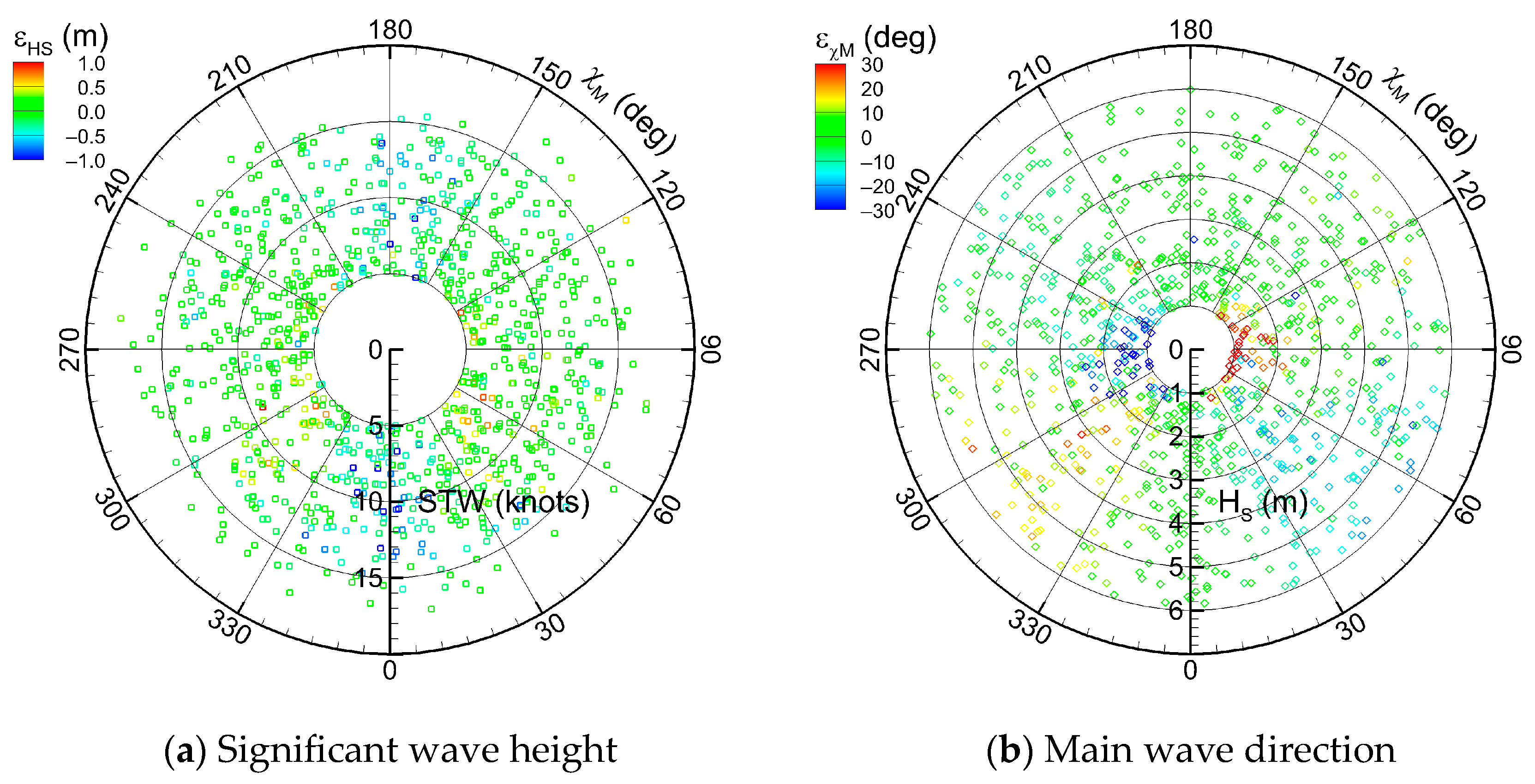
It is observed that each of the two regularization methods has an optimal hyperparameter range: (βχ, βω) = (−1~0, −1~0) for the bilinear method and βs = 1~2 for the B-spline method. Within these optimal ranges, the sea state estimation accuracy of the two methods is comparable, implying that the choice of interpolation and regularization schemes is not critical under the current two-dimensional directional spectrum resolution. Figure 14 shows the error distribution for the test dataset when the B-spline method is applied with the optimal hyperparameter βs = 1. The physics-based model generally produces accurate results over a wide range of sea states and ship operating conditions. Nevertheless, under certain circumstances, estimation errors increase. In low significant wave height conditions, the accuracy of the main wave direction decreases markedly, whereas under following sea conditions, errors in significant wave height increase, with the effect becoming more pronounced at higher ship speeds.
Unstable sea state estimation of the physics-based model is primarily attributed to the characteristics of wave-induced ship motions, and the error sources can be broadly categorized into two main factors. First, the ship exhibits small responses under low sea states. In mild ocean environments, wave heights are relatively small, and the energy is concentrated in the short-wave region. The ship acts as a low-pass filter because it is not significantly excited by short waves: high-frequency wave filtering. Extracting response characteristics, particularly inter-response relationships such as phase differences, from such small motions is inherently limited. Moreover, balancing the governing equations with regularization becomes increasingly challenging. Consequently, as shown in Figure 14b, below sea state 4 (HS < 1.88 m) the model fails to provide reliable estimates of wave directionality for oblique wave conditions. These uncertainties in low sea states represent a fundamental limitation of physics-based WBA models for large commercial ships.
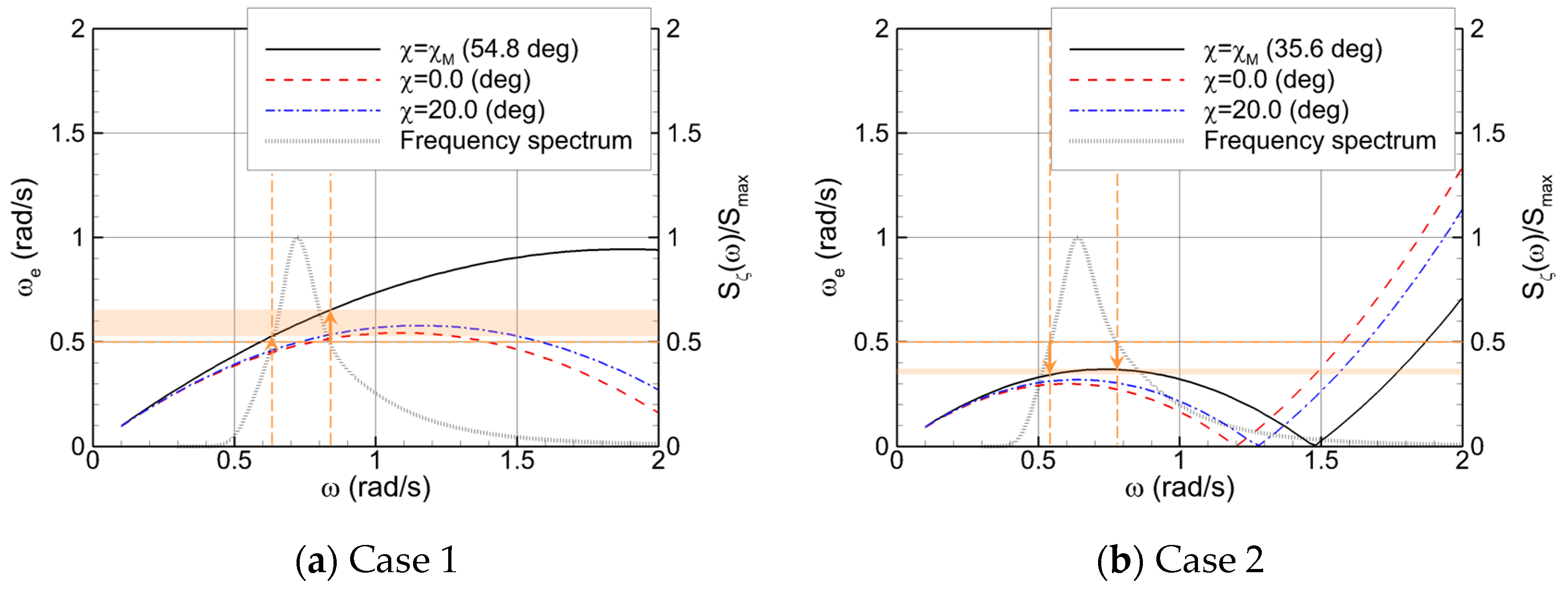
Second, errors arise from the relationship between absolute and encounter frequencies due to the Doppler effect. Figure 15 illustrates the frequency relationship for the following two test cases:
  • Case 1: GM = 1.9 m, STW = 8.77 knots, HS = 2.55 m, T2 = 7.81 s, χM = 54.8 deg
  • Case 2: GM = 3.2 m, STW = 15.9 knots, HS = 3.03 m, T2 = 8.06 s, χM = 35.6 deg
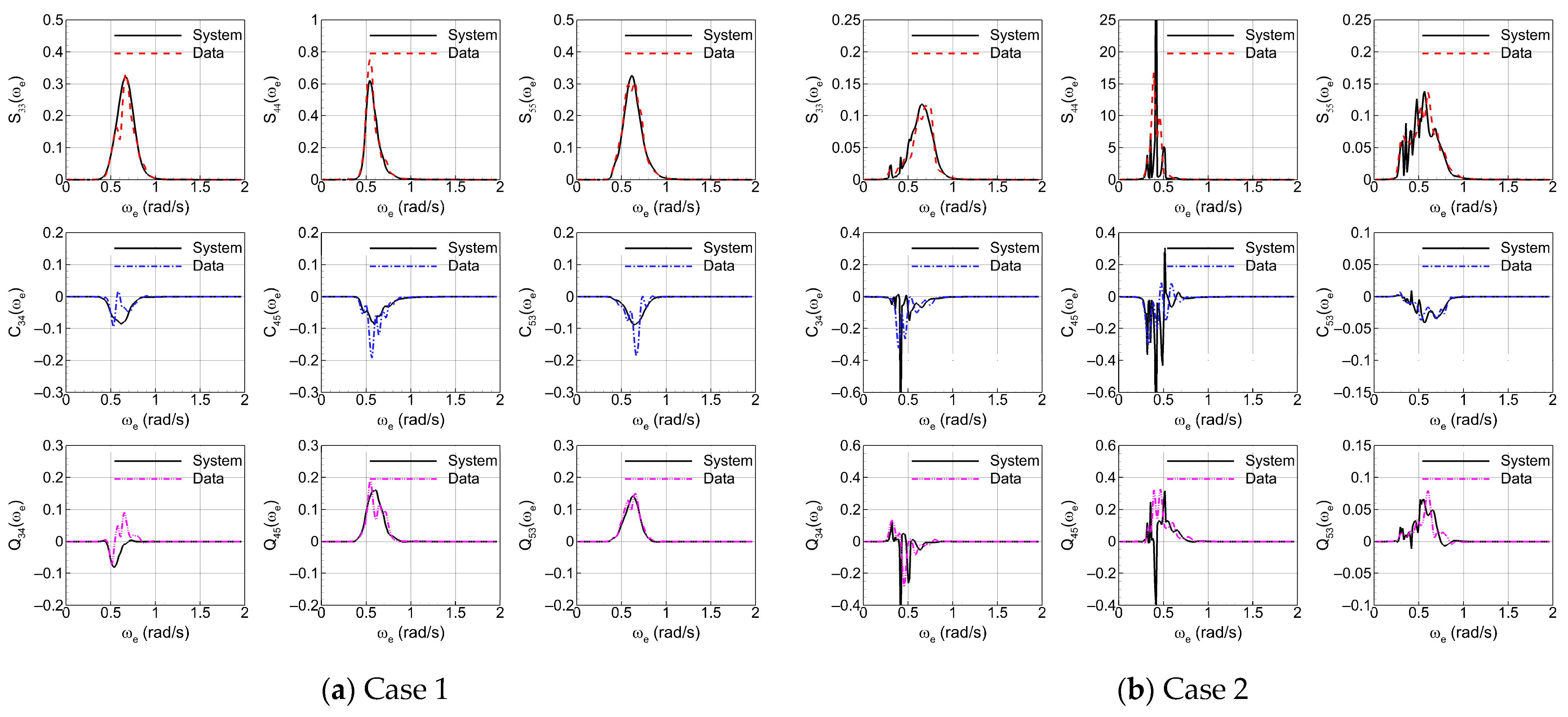
The two representative cases correspond to conditions of following seas, where the frequency relationship causes significant errors in sea state estimation, particularly reducing the accuracy in wave-direction estimation: for Case 1, χM,estimation = 31.1 deg, for Case 2, χM,estimation = 19.2 deg. In the figure, the shaded orange box highlights the encounter frequency range in the main wave direction, where the spectral ratio (Sζ(ω)/Smax) exceeds 0.5, denoting the dominant narrow-band motion response frequencies. Figure 16 shows the ship motion spectra induced by the wave spectrum in each case.
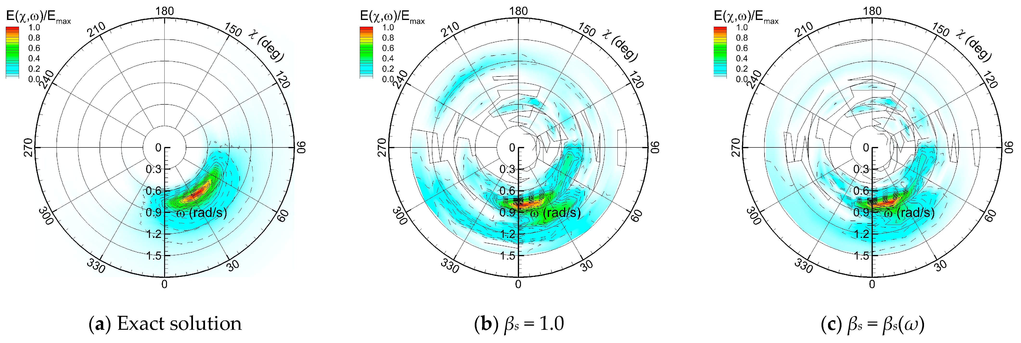
As shown in Figure 15a, because of the forward speed, high absolute frequencies can correspond to the dominant encounter frequencies in the following sea direction, which are not aligned with the main wave direction. In this high-frequency range (ω = 1.0~1.5 rad/s), the magnitude of the motion RAO is small, and its phase varies abruptly with frequency (see Figure 9), which may lead to overfitting to nonphysical wave components during the optimization process. Consequently, as shown in Figure 17b, the two-dimensional directional spectrum for Case 1, obtained with the physics-based model, exhibits an overestimation of wave energy at the model’s high-frequency degrees-of- freedom in the following sea direction. Errors in the main wave direction resulting from such overfitting can be observed in the stern-quartering sea test data in Figure 14b.
Furthermore, under high-speed following-sea conditions, as in Case 2, Figure 15b shows that the motion response becomes concentrated in the low encounter frequency range due to intensified Doppler effects. Such narrow-band responses pose challenges for spectral analysis, since the finitely discretized frequency domain leads to spectral leakage and increased uncertainty, as illustrated in Figure 16. Here, “System” refers to the motion spectra obtained by substituting the exact directional wave spectrum into the governing equations, whereas “Data” denotes the results obtained by applying Welch’s method to a 30-min ship motion time series. Compared with Case 1, the motion spectra in Case 2 exhibit locally spiky characteristics due to the higher ship speed and following sea conditions, with greater discrepancies between the exact solution and the spectral analysis results. This phenomenon occurs because the frequency slope in Equation (3) diverges (a/e → ∞), indicating numerical instability in the physics-based model. Therefore, as shown in Figure 18b, accurately identifying wave directionality and redistributing energy across absolute frequencies within the 1-to-3 mapping becomes challenging. The increase in optimization error under following sea conditions can also be confirmed in Figure 14a.
As a measure to address the optimization limitations, a frequency-dependent hyperparameter defined in Equation (12) is introduced, rather than applying a constant value over the entire solution domain, to strongly penalize high-frequency overfitting. The rationale for introducing this piecewise function is that, for large commercial vessels (L > 200 m), WBA typically targets sea states above level 4, and the operating speed is generally below 20 knots. Accordingly, considering the relationship between absolute and encounter frequencies, the overfitted high-frequency range can be approximately identified. Specifically, at absolute frequencies above approximately 1.0 rad/s, where the ocean wave energy is substantially smaller, any overestimated components are likely nonphysical. In this study, a simple functional form is adopted; however, any function that gradually increases the degree of regularization with frequency could also suffice. By introducing the frequency-dependent hyperparameter, the reconstructed directional wave spectra are stabilized by mitigating the nonphysical high-frequency energy, and accuracy with respect to the exact solution is improved, as shown in Figure 17c and Figure 18c. Finally, the overall performance of the physics-based model across the entire test dataset is summarized in Table 5, demonstrating that incorporating βs(ω) enhances the model’s accuracy and reliability for all sea state parameters. In particular, the estimation errors for the peak period and peak direction, which represent the dominant components of wave energy, are significantly reduced.

3.3. Results of Machine Learning Model

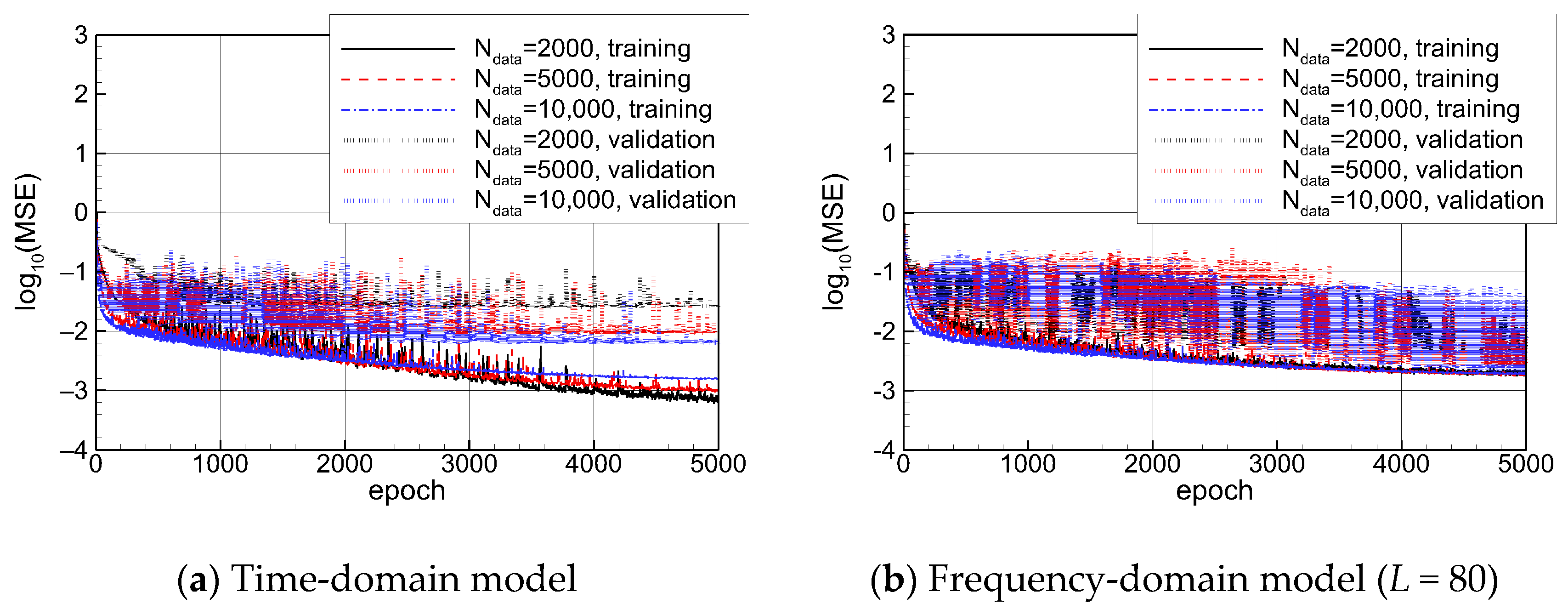
The machine learning models are trained using the ship motion dataset defined in Table 3. Figure 19 illustrates the training process of both the time-domain and frequency-domain models. As described in Section 2.3, the time-domain model directly uses time series as input, whereas the frequency-domain model extracts selected spectral components of the motion responses. The entire dataset is divided into training and validation subsets with a ratio of 4:1. The mean squared error as a function of epochs shows that optimization converges at approximately 5000 epochs. For the time-domain model, as the total dataset size Ndata increases, the converged MSE for the training dataset becomes larger, whereas that for the validation dataset decreases. This indicates a tendency toward overfitting for the time-domain model. In contrast, the frequency-domain model exhibits less sensitivity to the total dataset size, and the converged MSE values for both the training and validation sets are similar. Although the loss function for the validation set exhibits significant oscillations, the learning process demonstrates that the model achieves good generalization. As a result, the performance on the validation set is superior in the frequency-domain model compared to the time-domain model, whereas the opposite trend is observed for the training set. All subsequent results are obtained using models trained with 10,000 samples.
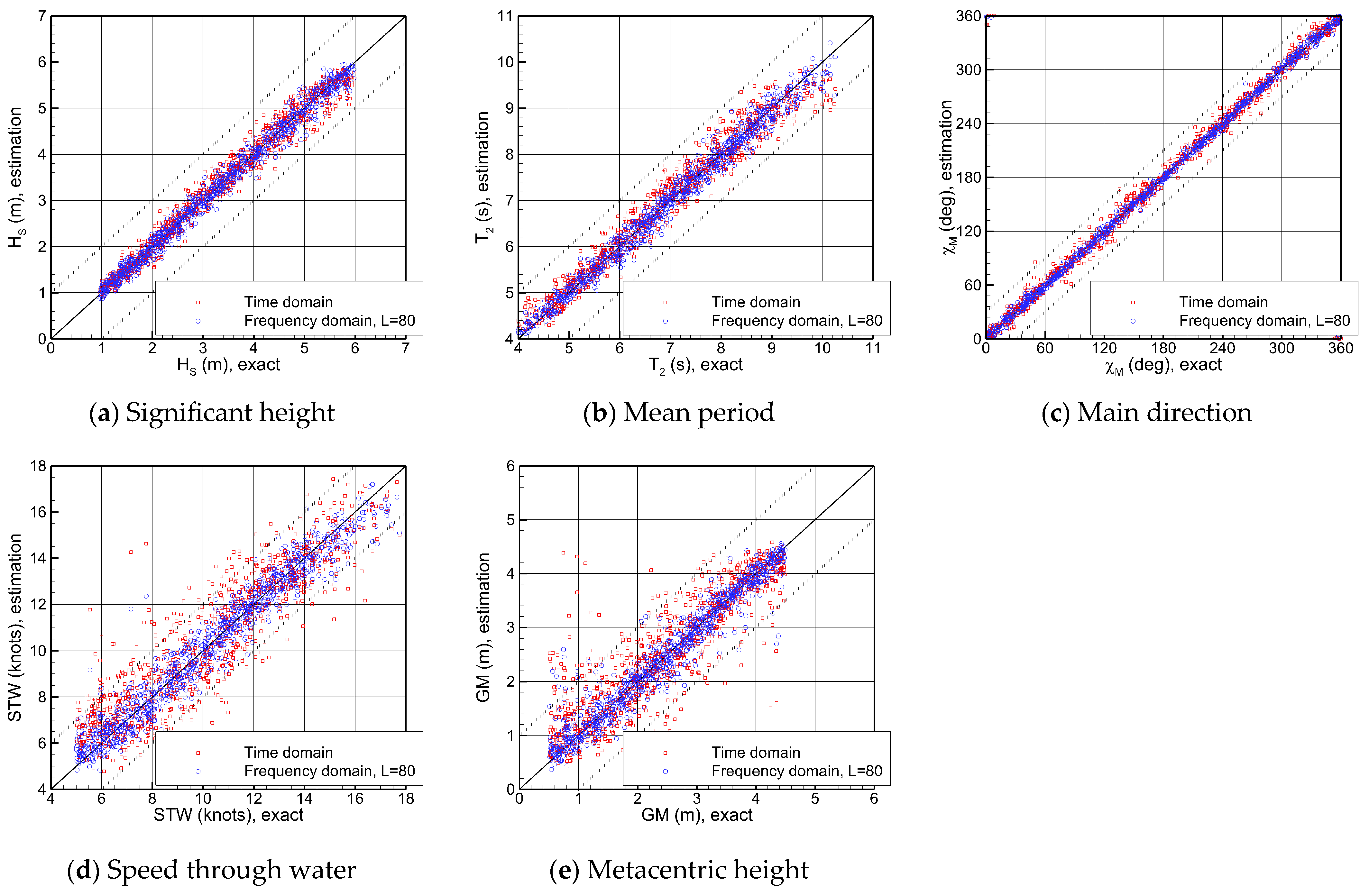
The inference of the machine learning models is performed on 1000 test samples, identical to those used for the physics-based model. As shown in Figure 20, the frequency-domain model provides more accurate and less scattered estimates than the time-domain model for all output variables, which is consistent with the training results. Each model incorporates different measures to enhance generalization. For the time-domain model, average pooling is applied to smooth the time series and mitigate overfitting to noise. In the frequency-domain model, stabilized input data are constructed through power spectral density (PSD) averaging in Welch’s method during spectral analysis. The testing results suggest that refining ship motion information prior to input, as in the frequency-domain case, leads to greater improvement in model generalization. On the other hand, for ship operating conditions, the errors in both models are larger relative to the variable ranges compared than those of the sea state parameters, and the performance gap between the two models is also more pronounced. In particular, the time-domain model fails to infer ship speed and GM in some test cases. Since the operating conditions influence the ship’s seakeeping dynamics indirectly, compared with ocean environmental conditions, extracting operational information implicitly embedded in the time series or spectral data is inherently more challenging than estimating sea state parameters.
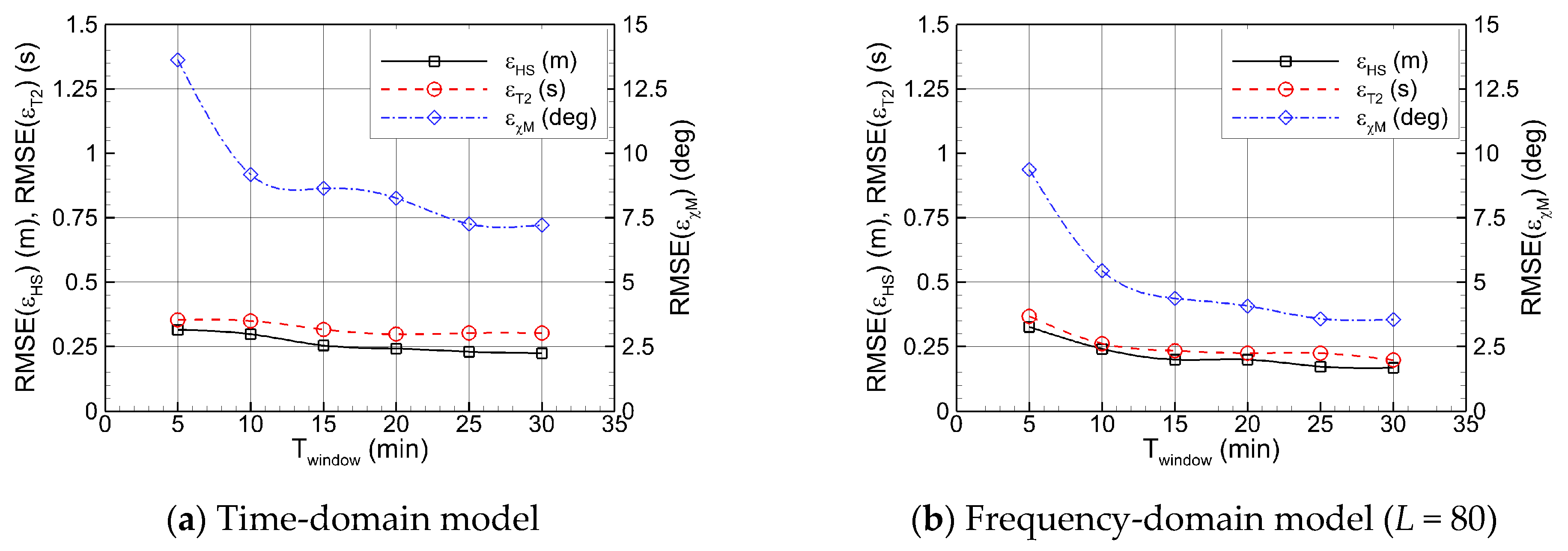
To analyze the model performance more closely, the RMSE over the entire test dataset is compared with respect to the length of the ship motion time window. The frequency-domain models are constructed using three different numbers of frequency components, L = 40, 80, and 160 (Δωe = π/64, π/128, and π/256). As shown in Figure 21, shorter time windows lead to higher training efficiency, but with less motion information available to the model, the estimation accuracy for sea state parameters is reduced. In particular, since the complexity of the frequency-domain model (the number of weights) remains constant regardless of the time window length, the model is more prone to overfitting when limited information is provided. Moreover, when Welch’s method is applied to short time windows, the variance of the PSD increases. Consequently, the model is trained on statistically unconverged data with high spectral uncertainty, leading to degraded performance. This tendency is more evident for wave direction than for wave height or period, and the errors converge when the time window exceeds approximately 25 min. As illustrated in Figure 22, the inference of ship operational information shows the same tendency with respect to time window length. However, the model performance shows little sensitivity to the number of frequency components, i.e., the spectral resolution.
Figure 23 presents the performance of the frequency-domain model across different ranges of sea states and ship operating conditions. The RMSE in each interval is normalized by the values over the entire test dataset. The estimation results for various sea state conditions show trends consistent with the physics-based model (see the top panel of Figure 23). (1) For sea states lower than 4, the error in wave direction increases. (2) Under following-sea conditions, the accuracy of significant wave height and mean period decreases. This indicates that the machine learning model, similar to the physics-based model, also struggles to identify salient features from the input data when the motion responses are weak or when narrow-band frequency focusing occurs due to the Doppler effect. However, unlike the physics-based model, the performance degradation under these conditions is less significant. Even under conditions of HS < 1.88 m, the RMSE of wave direction estimation remains below 5 degrees, demonstrating high accuracy (see Table 6). This indicates that the machine learning model can be applied to sea state estimation across the overall wave height range, and its performance is expected to improve as more training datasets become available. In contrast, for ship operational information, the error nearly doubles under low wave height conditions. In particular, GM, which is closely related to roll motion, can be estimated more accurately in beam-sea conditions than in head or following seas. This suggests that when motion responses are weak in mild sea states, the extraction of operational information is limited in applicability. Meanwhile, when comparing the errors by ship speed and GM ranges, the difference in model performance is not evident (see the bottom panel of Figure 23). It should be noted that the increase in errors for the high-speed interval (15 knots < STW < 20 knots) is mainly due to the fact that high-speed operations are accompanied by low wave heights, resulting in small motion responses.
Table 6 summarizes the overall errors of the machine learning models. When the models are trained with datasets covering the same ranges of operating conditions as those in the test dataset, their performance exceeds that of the physics-based model (see Table 5). However, in actual ship motion databases, operating conditions are not uniformly distributed. For example, GM often exhibits locally concentrated distributions depending on specific loading conditions. In this study, to analyze the performance of models trained within restricted operating condition ranges, narrow-range ship motion databases are constructed as shown in Figure 24. The details of each database are as follows:
  • DB 1: STW ∈ [5, 6] ∪ [10, 11] ∪ [15, 16] ∪ [17, ∞] knots
  • DB 2: GM ∈ [0.5, 0.75] ∪ [2.0, 2.5] ∪ [4.25, 4.5] m
  • DB 3: (STW ∈ [5, 7] ∪ [10, 12] ∪ [15, ∞] knots) ∩ (GM ∈ [0.5, 1.0] ∪ [2.0, 3.0] ∪ [4.0, 4.5] m)
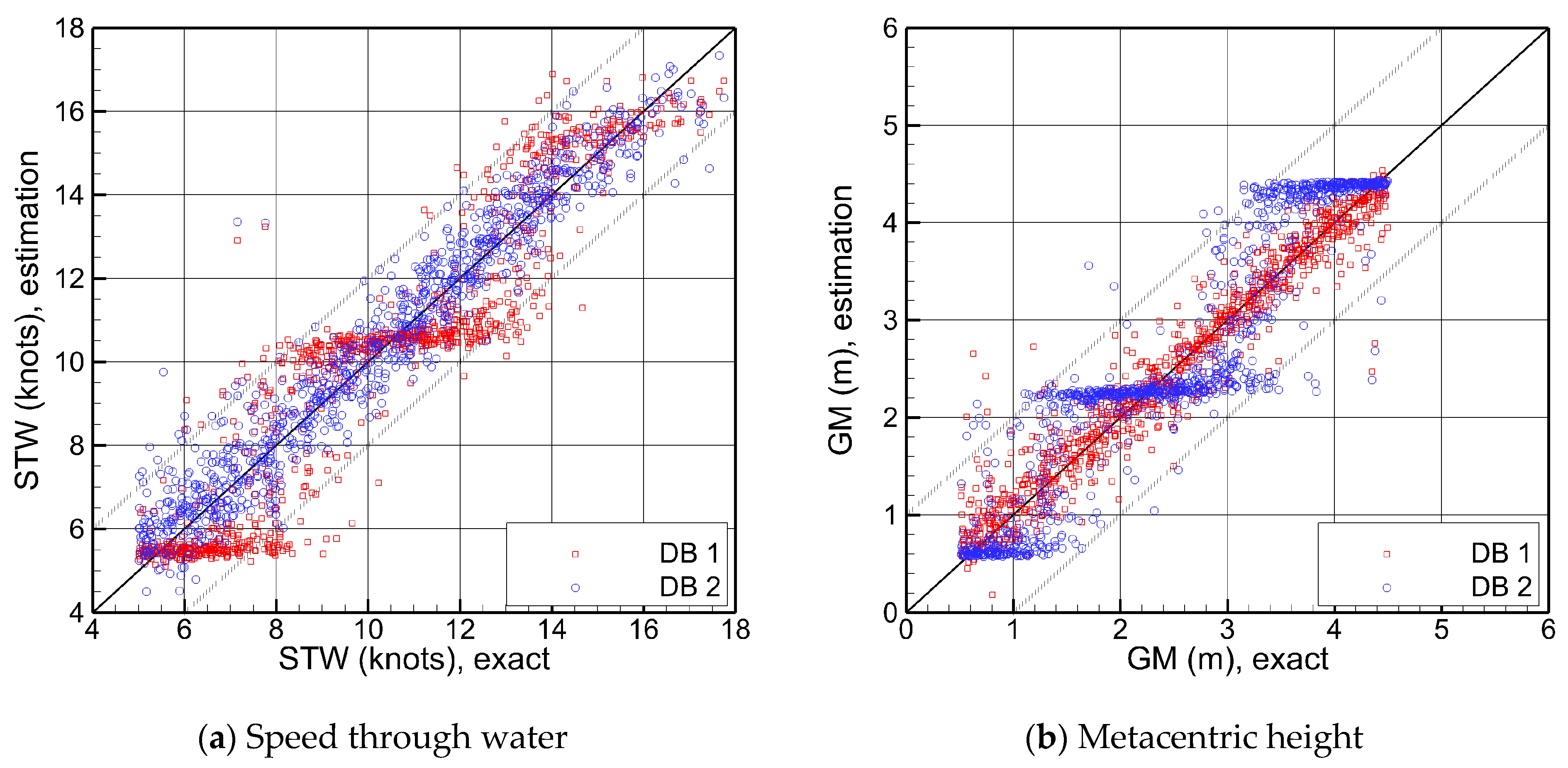
It should be noted that the machine learning models for these databases are also trained with the same number of data (10,000 samples) Figure 25 presents the performance of each model trained on a narrow-range database on the test dataset. The RMSE is computed separately for in-range test data, which fall within the training condition ranges, and out-of-range test data, which fall outside, and normalized with respect to the model trained on the full-range dataset. For sea state parameters, the errors for out-of-range test data are slightly larger than those for in-range data, but the discrepancy is not significant. This implies that sea-state estimation is feasible even for ship motion data corresponding to unseen operating conditions during training. In other words, ship motion dynamics do not vary drastically with operating conditions, and such variations can be adequately interpolated by the machine learning model. Consequently, a sea state estimation model can be developed even from databases with restricted condition ranges. In contrast, large errors occur in the inference of operating information for out-of-range test data. Figure 26 shows the estimation results of operating conditions using models trained on DB 1 and DB 2. The results confirm that each model is overfitted to its specific operating condition ranges, and thus, developing an operating condition estimation model is infeasible when relying on the biased databases.
In this study, the machine learning models are trained using data generated through numerical simulations. Therefore, it is possible to supply sufficient data across broad ranges of sea states and ship operating conditions, under which the models achieve superior performance to the physics-based models without limitations under certain conditions such as low wave heights or following seas. However, in real applications, it is not easy to secure a sufficiently large amount of ship operation data, and the available data may be concentrated in certain conditions. In such cases, the performance of machine learning models may deteriorate when exposed to unseen test conditions. The results of the present study regarding ML model training and testing under locally restricted ship operating conditions demonstrate this issue, highlighting that the most critical factor in developing machine learning models is not the model architecture but rather the availability of sufficiently comprehensive training datasets [35]. In the future, the application and performance validation of the machine learning model on real ship operational datasets must be conducted.
For WBA to function as a solution that provides safe ship operation guidance, real-time execution must be ensured. A trained machine learning model performs inference instantaneously. The nonparametric physics-based model in the present study can also estimate sea states for a 30-min motion time series within approximately 2 min and 40 s on an Intel i9-12900H/2.50 GHz CPU processor: (1) about 1 min and 40 s for defining and solving the equations of ship motions, (2) about 20 s for spectral analysis based on Welch’s method, and (3) about 40 s for nonparametric model setup and optimization. Therefore, both models can be applied in real time to recursively shifting time windows of ship motion responses.
For the development of a reliable WBA-based ship operational solution, the integration of sea state estimation from both physics-based and machine learning models is required. For typical sea states where sufficient datasets are available, machine learning models can be effectively applied, whereas in extreme and rare ocean environments, physics-based models should be employed. As verified in this study, physics-based models exhibit reduced performance under certain wave height and direction conditions, and their scope of application should therefore be restricted. In contrast, machine learning models should be incorporated into the solution based on the uncertainty of their outputs. Methods for uncertainty evaluation include measuring the relative position of test conditions with respect to the training data distribution using Euclidean distance or Mahalanobis distance, or assessing the variance among the predictions of multiple machine learning models [37]. Based on the evaluated uncertainty, the weighting between physics-based and machine learning models in the final estimation should be determined [36]. In conclusion, to establish an integration criterion considering applicability and uncertainty of each model, the performance of the models should be continuously monitored for real ship operational datasets.

4. Conclusions

In this study, both physics- and machine learning-based WBA models were developed and applied to a wide range of ship operating and sea-state conditions to evaluate their performance. A ship motion database was constructed through time-domain simulations for model training and testing. The comparison and analysis of the estimation results between the two approaches lead to the following conclusions:
  • For overall test conditions, the physics-based model provides accurate estimates of sea-state parameters. However, under low sea states with weak motion responses and in following sea conditions where narrow-band frequency focusing occurs, the optimization fails and the errors increase significantly. Introducing a frequency-dependent hyperparameter for the smoothness constraint alleviates optimization errors caused by the overfitting to high-frequency wave energy, thereby improving model performance.
  • When refined ship motion information obtained through spectral analysis is used as input, the machine learning model achieves higher accuracy and generalization performance compared with directly using raw time series data. In particular, the machine learning model can estimate both ship operating and sea state parameters with minimal error, even when the motion responses show ambiguous features that hinder the optimization of the physics-based model. When trained on biased databases with restricted operating condition ranges, the machine learning model can still estimate sea states but tends to overfit to specific ranges in the inference of ship operations without interpolation.
  • Both physics-based and machine learning models show limited sensitivity in performance across general ranges of ship operating conditions. Accordingly, machine learning models are well suited for test conditions where sufficient training data are available, whereas physics-based models remain necessary for extreme and rare ocean environmental conditions. To develop reliable WBA solutions in the future, it is essential to integrate the two models by incorporating their respective applicability uncertainty, when applied to motion response data obtained from actual ship operations.

Author Contributions

Conceptualization, J.-H.L., D.K. and J.-H.C.; methodology, J.-H.L.; software, J.-H.L.; validation, J.-H.L. and D.K.; formal analysis, J.-H.L.; investigation, J.-H.L.; resources, D.K. and J.-H.C.; data curation, J.-H.L.; writing—original draft preparation, J.-H.L.; writing—review and editing, D.K. and J.-H.C.; visualization, J.-H.L.; supervision, D.K. and J.-H.C.; project administration, D.K. and J.-H.C.; funding acquisition, J.-H.C. All authors have read and agreed to the published version of the manuscript.

Funding

This research received no external funding.

Data Availability Statement

The original contributions presented in this study are included in the article. Further inquiries can be directed to the corresponding author.

Acknowledgments

The authors would like to express their sincere gratitude to Yooil Kim and Researcher Jaehyeon Son of INHA University for their valuable advice and guidance on the theoretical aspects of the physics-based WBA model.

Conflicts of Interest

Authors Jae-Hoon Lee, Donghyeong Ko, and Ju-Hyuck Choi were employed by the company HD Hyundai Heavy Industries Co., Ltd.

References

  1. Erikstad, S.O. Designing ship digital services. In Proceedings of the 18th Conference on Computer and IT Applications in the Maritime Industries, Tullamore, Ireland, 25–27 March 2019. [Google Scholar]
  2. Giering, J.E.; Dyck, A. Maritime Digital Twin architecture: A concept for holistic Digital Twin application for shipbuilding and shipping. at—Automatis. 2021, 69, 1081–1095. [Google Scholar] [CrossRef]
  3. Lee, J.H.; Nam, Y.S.; Kim, Y.; Liu, Y.; Lee, J.; Yang, H. Real-time digital twin for ship operation in waves. Ocean Eng. 2022, 266, 112867. [Google Scholar] [CrossRef]
  4. Nieto-Borge, J.C.; Reichert, K.; Dittmer, J. Use of nautical radar as a wave monitoring instrument. Coast. Eng. 1999, 37, 331–342. [Google Scholar] [CrossRef]
  5. Hessner, K.; Reichert, K.; Dittmer, J.; Nieto-Borge, J.C.; Gunther, H. Evaluation of WAMOS II wave data. In Proceedings of the 4th International Symposium on Ocean Wave Measurement and Analysis, San Francisco, CA, USA, 2–6 September 2001. [Google Scholar]
  6. Dankert, H.; Rosenthal, W. Ocean surface determination from X-band radar-image sequences. J. Geophys. Res. 2004, 109, C04016. [Google Scholar] [CrossRef]
  7. Tannuri, E.A.; Sparano, J.V.; Simos, A.N.; Da Cruz, J.J. Estimating directional wave spectrum based on stationary ship motion measurements. Appl. Ocean Res. 2003, 25, 243–261. [Google Scholar] [CrossRef]
  8. Nielsen, U.D.; Stredulinsky, D.C. Sea state estimation from an advancing ship—A comparative study using sea trial data. Appl. Ocean Res. 2012, 34, 33–44. [Google Scholar] [CrossRef]
  9. Montazeri, N.; Nielsen, U.D.; Jensen, J.J. Estimation of wind sea and swell using shipboard measurements—A refined parametric modelling approach. Appl. Ocean Res. 2016, 54, 73–86. [Google Scholar] [CrossRef]
  10. Piscopo, V.; Scamardella, S.; Gaglione, S. A new wave spectrum resembling procedure based on ship motion analysis. Ocean Eng. 2020, 201, 107137. [Google Scholar] [CrossRef]
  11. Zago, L.; Simos, A.N.; Kawano, A.; Kogishi, A.M. A new vessel motion based method for parametric estimation of the waves encountered by the ship in a seaway. Appl. Ocean Res. 2023, 134, 103499. [Google Scholar] [CrossRef]
  12. Park, M.J.; Kim, Y. Probabilistic estimation of directional wave spectrum using onboard measurement data. J. Mar. Sci. Technol. 2024, 29, 200–220. [Google Scholar] [CrossRef]
  13. Iseki, T.; Ohtsu, K. Bayesian estimation of directional wave spectra based on ship motions. Control Eng. Pract. 2000, 8, 215–219. [Google Scholar] [CrossRef]
  14. Nielsen, U.D. Estimations of on-site directional wave spectrum from measured ship responses. Mar. Struct. 2006, 19, 33–69. [Google Scholar] [CrossRef]
  15. Pascoal, R.; Soares, C.G. Non-parametric wave spectral estimation using vessel motions. Appl. Ocean Res. 2008, 30, 46–53. [Google Scholar] [CrossRef]
  16. Souza, F.L.; Tannuri, E.A.; Mello, P.C.; Franzini, G.; Mas-Soler, J.; Simos, A.N. Bayesian Estimation of Directional Wave-Spectrum Using Vessel Motions and Wave-Probes: Proposal and Preliminary Experimental Validation. J. Offshore Mech. Arct. Eng. 2018, 140, 041102. [Google Scholar] [CrossRef]
  17. Nielsen, U.D.; Dietz, J. Ocean wave spectrum estimation using measured vessel motions from an in-service container ship. Mar. Struct. 2020, 69, 102682. [Google Scholar] [CrossRef]
  18. Lee, C.; Kim, Y. Local response estimation of a seagoing vessel using onboard measurement data. Mar. Struct. 2022, 86, 103298. [Google Scholar] [CrossRef]
  19. Nielsen, U.D.; Mittendorf, M.; Shao, Y.; Storhaug, G. Wave spectrum estimation conditioned on machine learning-based output using the wave buoy analogy. Mar. Struct. 2023, 91, 103470. [Google Scholar] [CrossRef]
  20. Nielsen, U.D. Introducing two hyperparameters in Bayesian estimation of wave spectra. Probab. Eng. Mech. 2008, 23, 84–94. [Google Scholar] [CrossRef]
  21. Bispo, I.B.S.; Simos, A.N.; Tannuri, E.A.; Cruz, J.J. Motion-based Wave Estimation by a Bayesian Inference Method: A Procedure for Pre-defining the Hyperparameters. In Proceedings of the 22nd International Offshore and Polar Engineering Conference, Rhodes, Greece, 17–22 June 2012. [Google Scholar]
  22. Nielsen, U.D. A concise account of techniques available for shipboard sea state estimation. Ocean Eng. 2017, 129, 352–362. [Google Scholar] [CrossRef]
  23. Nielsen, U.D.; Bingham, H.B.; Brodtkorb, A.H.; Iseki, T.; Jensen, J.J.; Mittendorf, M.; Mounet, R.E.G.; Shao, Y.; Storhaug, G.; Sorensen, A.J.; et al. Estimating waves via measured ship responses. Sci. Rep. 2023, 13, 17342. [Google Scholar] [CrossRef] [PubMed]
  24. Nielsen, U.D. Transformation of a wave energy spectrum from encounter to absolute domain when observing from an advancing ship. Appl. Ocean Res. 2017, 69, 160–172. [Google Scholar] [CrossRef]
  25. Nielsen, U.D. Deriving the absolute wave spectrum from an encountered distribution of wave energy spectral densities. Ocean Eng. 2018, 165, 194–208. [Google Scholar] [CrossRef]
  26. Mak, B.; Duz, B. Ship as a Wave Buoy: Estimating Relative Wave Direction from In-Service Ship Motion Measurements Using Machine Learning. In Proceedings of the 38th International Conference on Ocean, Offshore, and Arctic Engineering, Glasgow, UK, 9–14 June 2019. [Google Scholar]
  27. Kawai, T.; Kawamura, Y.; Okada, T.; Mitsuyuki, T.; Chen, X. Sea state estimation using monitoring data by convolutional neural network (CNN). J. Mar. Sci. Technol. 2021, 26, 947–962. [Google Scholar] [CrossRef]
  28. Mittendorf, M.; Nielsen, U.D.; Bingham, H.B.; Storhaug, G. Sea state identification using machine learning—A comparative study based on in-service data from a container vessel. Mar. Struct. 2022, 85, 103274. [Google Scholar] [CrossRef]
  29. Selimovic, D.; Hrzic, F.; Prpic-Orsic, J.; Lerga, J. Estimation of sea state parameters from ship motion responses using attention-based neural networks. Ocean Eng. 2023, 381, 114915. [Google Scholar] [CrossRef]
  30. Cheng, X.; Li, G.; Skulstad, R.; Chen, S.; Hildre, H.P.; Zhang, H. Modeling and Analysis of Motion Data from Dynamically Positioned Vessels for Sea State Estimation. In Proceedings of the 2019 International Conference on Robotics and Automation, Montreal, ON, Canada, 20–24 May 2019. [Google Scholar]
  31. Cheng, X.; Li, G.; Skulstad, R.; Zhang, H.; Chen, S. SpectralSeaNet: Spectrogram and Convolutional Network-based Sea State Estimation. In Proceedings of the 46th Annual Conference of the IEEE Industrial Electronics Society, Singapore, 18–21 October 2020. [Google Scholar]
  32. Scholcz, T.P.; Mak, B. Ship as a Wave Buoy—Estimating Full Directional Wave Spectra from In-Service Ship Motion Measurements Using Deep Learning. In Proceedings of the 39th International Conference on Ocean, Offshore, and Arctic Engineering, Fort Lauderdale, FL, USA, 28 June–3 July 2020. [Google Scholar]
  33. Han, P.; Li, G.; Skjong, S.; Zhang, H. Directional wave spectrum estimation with ship motion responses using adversarial networks. Mar. Struct. 2022, 83, 103159. [Google Scholar] [CrossRef]
  34. Cheng, X.; Li, G.; Ellefsen, A.L.; Chen, S.; Hildre, H.P.; Zhang, H. A Novel Densely Connected Convolutional Neural Network for Sea-Sate Estimation Using Ship Motion Data. IEEE Trans. Instrum. Meas. 2020, 69, 5984–5993. [Google Scholar] [CrossRef]
  35. Nielsen, U.D.; Iwase, K.; Mounet, R.E.G. Comparing machine learning-based sea state estimates by the wave buoy analogy. Appl. Ocean Res. 2024, 149, 104042. [Google Scholar] [CrossRef]
  36. Han, P.; Li, G.; Cheng, X.; Skjong, S.; Zhang, H. An Uncertainty-Aware Hybrid Approach for Sea State Estimation Using Ship Motion Responses. IEEE Trans. Ind. Informat. 2022, 18, 891–900. [Google Scholar] [CrossRef]
  37. Nielsen, U.D.; Iwase, K.; Mounet, R.E.G.; Storhaug, G. Uncertainty-associated directional wave spectrum estimation from wave-induced ship responses using machine learning methods. Ocean Eng. 2024, 313, 119543. [Google Scholar] [CrossRef]
  38. Bisinotto, G.A.; Sparano, J.V.; Simos, A.N.; Cozman, F.G.; Ferreira, M.D.; Tannuri, E.A. Sea state estimation based on the motion data of a moored FPSO using neural networks: An evaluation with multiple draft conditions. Ocean Eng. 2023, 276, 114235. [Google Scholar] [CrossRef]
  39. Bendat, J.S.; Piersol, A.G. Random Data—Analysis and Measurement Procedures, 3rd ed.; Wiley: New York, NY, USA, 2000. [Google Scholar]
  40. Ren, Z.; Han, X.; Verma, A.S.; Dirdal, J.A.; Skjetne, R. Sea state estimation based on vessel motion responses: Improved smoothness and robustness using Bezier surface and L1 optimization. Mar. Struct. 2021, 76, 102904. [Google Scholar] [CrossRef]
  41. Son, J.; Kim, Y. Directional wave spectrum estimation through onboard measurement data utilizing B-spline basis functions. Ocean Eng. 2024, 313, 119679. [Google Scholar] [CrossRef]
  42. Cummins, W.E. The impulse response function and ship motions. Schiffstechnik 1962, 47, 101–109. [Google Scholar]
  43. Salvesen, N.; Tuck, E.O.; Faltinsen, O. Ship motions and sea loads. Trans. Soc. Nav. Archit. Mar. Eng. 1970, 78, 250–279. [Google Scholar]
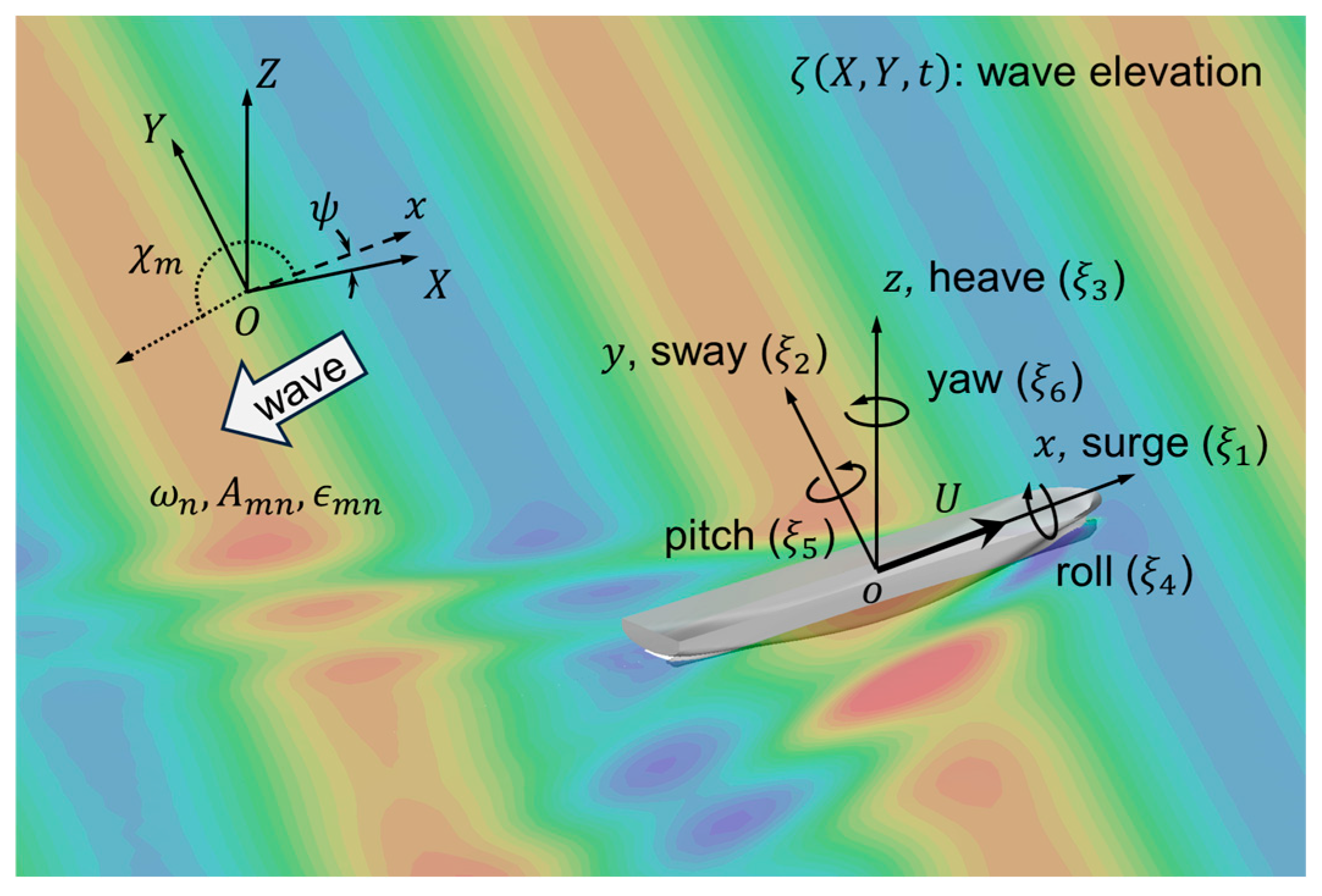
Figure 1. Coordinate systems and definitions.
Jmse 13 01823 g001
Figure 2. Relationship between absolute and encounter wave frequencies: U = 15 knots.
Jmse 13 01823 g002
Figure 3. Discretization in the nonparametric physics-based model.
Jmse 13 01823 g003
Figure 4. B-spline surface interpolation of the 2D directional wave spectrum.
Jmse 13 01823 g004
Figure 5. Hyperparameter configurations for the B-spline surface-based regularization.
Jmse 13 01823 g005
Figure 6. Input data for the machine learning model: ship motion time series and spectra.
Jmse 13 01823 g006
Figure 7. CNN architectures for time-domain (left) and frequency-domain (right) input data.
Jmse 13 01823 g007
Figure 8. Distribution of ship operating and sea state conditions in the ship motion database.
Jmse 13 01823 g008
Figure 9. Ship motion RAOs: GM = 4.1 m, STW = 15.0 knots.
Jmse 13 01823 g009
Figure 10. Sea state estimation with the physics-based model: bilinear method.
Jmse 13 01823 g010
Figure 11. Sea state estimation with the physics-based model: B-spline method.
Jmse 13 01823 g011
Figure 12. Comparison of the frequency spectra and directional spreading functions under different hyperparameters: GM = 3.3 m, STW = 6.04 knots, HS = 3.74 m, T2 = 7.81 s, χM = 277.8 deg.
Jmse 13 01823 g012
Figure 13. Root mean squared error (RMSE) of the physics-based model with difference hyperparameters.
Jmse 13 01823 g013
Figure 14. Error distribution of sea state estimation with the physics-based model: B-spline method.
Jmse 13 01823 g014
Figure 15. Relationship between absolute and encounter wave frequencies and the frequency spectrum.
Jmse 13 01823 g015
Figure 16. Comparison of ship motion spectra for different test cases: Twindow = 30 min.
Jmse 13 01823 g016
Figure 17. Comparison of two-dimensional directional spectrum estimates: Case 1.
Jmse 13 01823 g017
Figure 18. Comparison of two-dimensional directional spectrum estimates: Case 2.
Jmse 13 01823 g018
Figure 19. Mean squared error (MSE) in the training process: Twindow = 30 min.
Jmse 13 01823 g019
Figure 20. Sea state and ship operating condition estimation with the machine learning model.
Jmse 13 01823 g020
Figure 21. Root Mean squared error (RMSE) of sea state parameter estimates by the machine learning model with different time windows.
Jmse 13 01823 g021
Figure 22. Root Mean squared error (RMSE) of ship operating condition estimates by the machine learning model with different time windows.
Jmse 13 01823 g022
Figure 23. Root Mean squared errors (RMSEs) across condition ranges: for different sea states (top) and for different ship operation conditions (bottom), obtained with the frequency-domain machine learning model (Twindow = 30 min, L = 80).
Jmse 13 01823 g023
Figure 24. Ship motion databases with restricted ship operating condition ranges.
Jmse 13 01823 g024
Figure 25. Root Mean squared errors (RMSEs) for different training databases with restricted condition ranges, obtained with the frequency-domain machine learning model (Twindow = 30 min, L = 80).
Jmse 13 01823 g025
Figure 26. Ship operating condition estimation with the frequency-domain machine learning models trained on different training databases with restricted condition ranges (Twindow = 30 min, L = 80).
Jmse 13 01823 g026
Table 1. Computational parameters for the physics-based model.
DesignationSpecifications
Wave encounter frequenciesL = 160, ωe ∈ [π/256, 5π/8] rad/s (Δωe = π/256 rad/s)
Wave
directions
Collocation pointM’ = 36, (Δχ = 10 deg)
Solution pointM’ = 18, (Δχ = 20 deg)
Wave absolute frequenciesN = 27, ω ∈ [0.2, 1.5] rad/s (Δω = 0.05 rad/s)
HyperparameterBilinear method(lnβχ, lnβω) = (−3, −3), (−2, −2), …, (2, 2)
B-spline methodlnβs = −1, 0, …, 4 or βs(ω)
Table 2. Principal dimensions of the KCS containership model.
DesignationSpecifications
Length L230.0 m
Breadth B32.2 m
Depth D19.0 m
Design loading conditionDraft T10.8 m
Metacentric height GM0.6 m
Design speed U24.0 knots (Fn = 0.260)
Table 3. Test conditions adopted for the ship motion database.
DesignationSpecifications
Loading
condition
Draft T10.8 m
Metacentric height GM[0.5, 4.5] m
Navigational conditionSpeed through water STW[5, 21–(gHS)1/2] knots
Wave condition
(sea state parameters)
Significant height HS[1.0, 6.0] m
Peak period Tp/HS(1/2)[4.5, 5.5]
Main direction χM[0, 360] deg
Peak enhancement factor γ[1.0, 3.3]
(from PM to JONSWAP)
Spreading parameter smax[10.0, 25.0]
(from wind waves to swell)
Table 4. Specifications of the ship seakeeping database.
DesignationSpecifications
Ship speeds (STW)U ∈ [0, 25] knots (ΔU = 2.5 knots)
Wave directionsχ ∈ [0, 360] deg (Δχ = 5 deg)
Wave frequenciesω ∈ [0.1, 5.0] rad/s (Δω = 0.02 rad/s)
Table 5. Sea state estimation results: physics-based models.
B-Spline MethodRoot Mean Squared Error (RMSE)
εHS (m)εT2 (s)εχM (deg)εTp (s)εχp (deg)
βs = 1.0HS < 1.88 m0.185 0.517 27.8 0.878 42.7
HS ≥ 1.88 m0.328 0.381 9.89 0.726 14.9
Total0.305 0.413 15.4 0.760 23.5
βs = βs(ω)HS < 1.88 m0.182 0.676 27.3 0.760 31.1
HS ≥ 1.88 m0.264 0.368 8.13 0.544 8.34
Total0.249 0.449 14.3 0.595 15.9
Table 6. Sea state and ship operating condition estimation results: machine learning models.
Machine Learning ModelRoot Mean Squared Error (RMSE)
εHS (m)εT2 (s)εχM (deg)εSTW (knots)εGM (m)
Time-domain
model
HS < 1.88 m0.1360.2309.421.550.856
HS ≥ 1.88 m0.2420.3196.521.230.450
Total0.2240.3037.221.310.559
Frequency-domain
model
HS < 1.88 m0.1190.1534.930.9800.434
HS ≥ 1.88 m0.1790.2083.100.6190.222
Total0.1680.1983.550.7090.279
Disclaimer/Publisher’s Note: The statements, opinions and data contained in all publications are solely those of the individual author(s) and contributor(s) and not of MDPI and/or the editor(s). MDPI and/or the editor(s) disclaim responsibility for any injury to people or property resulting from any ideas, methods, instructions or products referred to in the content.