Deep Learning-Based Wind Speed Retrieval from Sentinel-1 SAR Wave Mode Data

Abstract

Sea surface wind has been listed as an essential climate variable, playing crucial roles in regulating the global and regional weather and climate. Spaceborne synthetic aperture radar (SAR) has demonstrated the advantages in observing the wind field given its all-weather measurement capability. In this study, we present a convolutional neural network (CNN)-based framework for retrieving 10 m wind speed ($U_{10}$) from Sentinel-1 SAR wave mode (WV) imagery. The model is trained on SAR data acquired in 2017 using collocated ERA5 reanalysis wind vectors as the reference, with final performance evaluated against a temporally independent dataset from 2016 and in situ wind measurements. The CNN approach demonstrates improved retrieval accuracy compared to the conventional CMOD5.N-based result, achieving lower root mean square error (RMSE) and bias across both WV1 and WV2 incidence angle modes. Residual diagnostics show a systematic overestimation at low wind speeds and a slight underestimation at higher wind speeds. Spatial analyses of retrieval bias reveal regional variations, particularly in areas characterized by ocean swell or convective atmospheric activity, highlighting the importance of geophysical features in retrieval accuracy. These results support the viability of deep learning approaches for SAR-based ocean surface wind estimation and suggest a path forward for the development of more accurate, data-driven wind products suitable for both scientific research and operational marine forecasting.

1. Introduction

Sea surface wind are vital for a wide range of oceanic and atmospheric processes, including the generation and modulation of ocean currents and the regulation of air–sea fluxes of heat, moisture, and momentum [1,2,3,4,5]. Consistent wind observations are essential for operational weather forecasting, climate modeling, marine navigation, offshore engineering, fisheries management, and natural disaster response [6]. The in situ platforms such as moored buoys, research vessels, and coastal meteorological stations have been the primary means in measuring sea surface wind vectors [7]. While these observations provide accurate point measurements as critical validation sources, their spatial coverage is inherently limited [8]. The vast extent of the global oceans, together with the challenges associated with deploying and maintaining in situ platforms, lead to great observational gaps, especially in remote locations and/or under extreme conditions [9]. Satellite remote sensing techniques, including those based on scatterometers, synthetic aperture radar (SAR), and passive microwave radiometers, offer a powerful means of addressing these limitations [10]. The spaceborne sensors provide broad and consistent spatial coverage with regular revisit times over both open oceans and coastal zones. Moreover, first-hand observations could be gathered in polar regions and extreme events [11]. The integrated wind vector dataset has been fundamental in understanding global wind patterns and air–sea interactions across different spatial and temporal scales [12,13].

Among the various remote sensing sensors, active radars are the most widely employed technique. The typical wind vector inversion scheme for these active radar relies on an empirical geophysical model function (GMF) that relates radar observables to neutral wind vectors at the height of 10 m above the sea surface, of which C-band GMF might be the commonly used, given the continuous operation of the Advanced Scatterometers (ASCAT) dating back to 20 years ago [14]. Wind vector inversion from backscatter measurements is typically performed through a variational approach or a maximum likelihood estimation [15]. A common practice is to define a cost function that quantifies the discrepancy between measured and model-predicted NRCS values across multiple azimuth angles. The inversion process seeks the wind vector that minimizes this cost function [16]. It should be noted that such an inversion scheme for scatterometers exploit observations of multiple beams to resolve the unique wind vector solution.

While SAR measurements have been viewed complementary to scatterometers for finer-scale wind information, its retrieval scheme is quite different given its single-antenna configuration. The most commonly used approach in SAR wind inversion is to introduce an external wind direction from either numerical weather prediction (NWP) or other measurements. Many efforts have been devoted to inferring wind vector solely from SAR measurements without any external input. One kind of approach utilizes the wind streaks signature present on SAR images to approximate the local wind direction for wind speed retrieval [17,18]. However, the wind streaks are not always persistent over all the SAR images [19], making it difficult to fill in the gaps where these features are absent. Other methods focus on developing new variables from SAR observations to construct revised cost function. Doppler shift, as an indicator of the sea surface velocity, is found to exhibit strong correlations with wind vector that helps constrain the wind inversion as documented in [20]. Given the signed nature of Doppler shift, an external wind information is yet required to resolve the solution [20]. Other image spectrum related parameters are also exploited, together with radar backscattering coefficient, to propose a self-sufficient wind inversion scheme [21]. However, this method needs complicated SAR image cross-spectrum estimates and it only applied to small incidence angles as reported in [21].

In recent years, another type of wind inversion scheme from SAR measurements has emerged due to the development of artificial intelligence and deep learning methods. Models such as convolutional neural networks (CNNs) and Residual Networks (ResNets) are capable of learning complex spatial patterns associated with wind fields directly from SAR images, without relying on explicit atmospheric features or external data [22,23,24]. These data-driven approaches have shown potential in resolving fine-scale wind variability and performing well in challenging scenarios such as convective storms or coastal zones. The applicability of such approaches to extensive SAR images over the global open ocean has yet to be addressed. In this study, we take advantage of the wave mode imagettes acquired by Sentinel-1 mission over the vast ocean basins, together with the CNN technique, to establish a straightforward wind speed inversion model. The proposed model is evaluated and validated against in situ reference observations. The paper is organized as follows. Section 2 describes the data and methodology. Section 3 presents the model training and the sensitivity analyses of key hyperparameters. Section 4 provides quantitative comparisons between CNN-based retrievals and traditional CMOD5.N results, along with validation using independent buoy data, followed by the Summary in Section 5.

2. Data and Methods

2.1. S-1 SAR Data

The Sentinel-1 (S-1) mission, launched within the European Space Agency’s Copernicus program, carries a C-band synthetic aperture radar operating at 5.405 GHz. The mission comprises three satellites, S-1A, S-1B, and S-1C, launched in 2014, 2016, and 2024, respectively. S-1A and S-1C remain active, while S-1B ceased operations at the end of 2022. The SAR system supports four imaging modes—Interferometric Wide Swath (IW), Extra Wide Swath (EW), Stripmap (SM), and Wave mode (WV)—with each corresponding to distinct observational objectives. WV mode is specifically designed for ocean surface monitoring, including measurements of wave spectra and wind fields. In this mode, the instrument acquires small vignettes (20 km × 20 km) at ∼100 km intervals along the satellite ground track. These scenes are collected alternately using two incidence angles: WV1 (∼23°) and WV2 (∼36°).

In this study, the 2017 dataset is used for model development and partitioned into training, validation, and test subsets using a 6:2:2 split. The training set was used for model weight optimization, while the validation set was used for hyperparameter tuning and to prevent overfitting. The 2017 test set provided a preliminary assessment of generalization on unseen data from the same year. To ensure a robust and unbiased evaluation of the final model performance, we used the data from July to December in 2016 as an independent hold-out test set, ensuring a complete temporal separation between model development and final validation. These data were excluded from the training process but exhibit comparable backscatter characteristics [25]. Figure 1a,b present the monthly distribution of WV1 and WV2 SAR acquisitions, respectively. Image count remained consistent throughout the study period, with no significant data gaps. Monthly acquisition counts generally exceed 20,000 scenes, supporting robust statistical analysis and model training. Figure 1c,d show the spatial distribution of SAR observations on a 2° × 2° grid for WV1 and WV2, respectively. Observation density is highest in the tropical and subtropical ocean basins, including the Intertropical Convergence Zone, the western Pacific, the Indian Ocean, and the Southern Ocean storm tracks. These spatial patterns reflect the S-1 orbital configuration and the wave mode acquisition strategy, which prioritizes regions with frequent dynamic ocean activity. In contrast, the Atlantic Ocean shows lower sampling density due to acquisition priority of the wide swath images in that region. Note that the orange stripes in the spatial map is an outcome of the Sentinel-1 WV leap-frog sampling strategy: it collects a SAR vignette every 200 km along the satellite track for a given incidence angle.

2.2. ERA5 Winds

The ERA5 surface wind vector data from the European Center for Medium-Range Weather Forecasts (ECMWF) are employed as background wind fields for the SAR-based inversion. ERA5 integrates a wide range of satellite and in situ observations through data assimilation, providing improved accuracy in surface wind representation [26]. The dataset offers global coverage with a spatial resolution of 0.25° × 0.25° and a temporal resolution of 1 h, enabling detailed characterization of wind speed and direction across spatial and temporal scales [27]. In this analysis, collocation between SAR observations and ERA5 wind fields is conducted by identifying the nearest neighbor in both space and time for each SAR acquisition [28]. Figure 1e,f show the probability density functions (PDFs) of collocated ERA5 10 m wind speed ($U_{10}$) for WV1 and WV2 modes, respectively. Wind speeds are binned at 0.5 m/s intervals. The resulting PDFs exhibit a unimodal distribution with a peak near 7.5 m/s, consistent with long-term global mean wind speeds over open-ocean regions [29]. The 2016 (solid blue lines) and 2017 (dashed red lines) distributions are closely aligned for both modes, indicating interannual consistency in wind speed conditions during the SAR acquisition periods. Small deviations are observed in the upper tail (>12 m/s), particularly for WV2 where the 2017 data show a higher frequency of strong wind events. These differences may reflect seasonal variability or interannual changes in the occurrence of high-wind conditions.

2.3. In Situ Buoy Observations

In this study, surface wind vector measurements collected by different sources and managed within the framework of Copernicus are used as independent ground truth reference data to assess the accuracy of wind retrievals from the established CNN model applied to Sentinel-1 SAR wave mode observations. Buoy-based wind measurements are usually recorded at height of 4 m above the sea level, which are transformed to wind speed at 10 m height with assumption of neutral atmospheric conditions. The buoy data are collocated with SAR image acquisitions using both spatial and temporal criteria. Specifically, SAR scenes are selected if the image center falls within a 80 km radius of the buoy locations, and the acquisition times differ by no more than 30 min from the buoy observation time. This spatiotemporal collocation ensures that the compared wind fields reflect approximately the same atmospheric state. For WV1 acquisitions, 65 distinct buoys yielded a total of 699 collocated SAR–buoy matchups. For WV2, 69 buoys provided 621 collocations. The buoy locations span a broad range of oceanic positions and this extensive geographic distribution allows the validation to encompass a wide variety of sea state and atmospheric conditions. Such diversity in validation conditions enhances the robustness of the statistical performance metrics derived from the comparison, ensuring that the evaluation captures model behavior across a representative spectrum of wind regimes.

2.4. Model Architecture

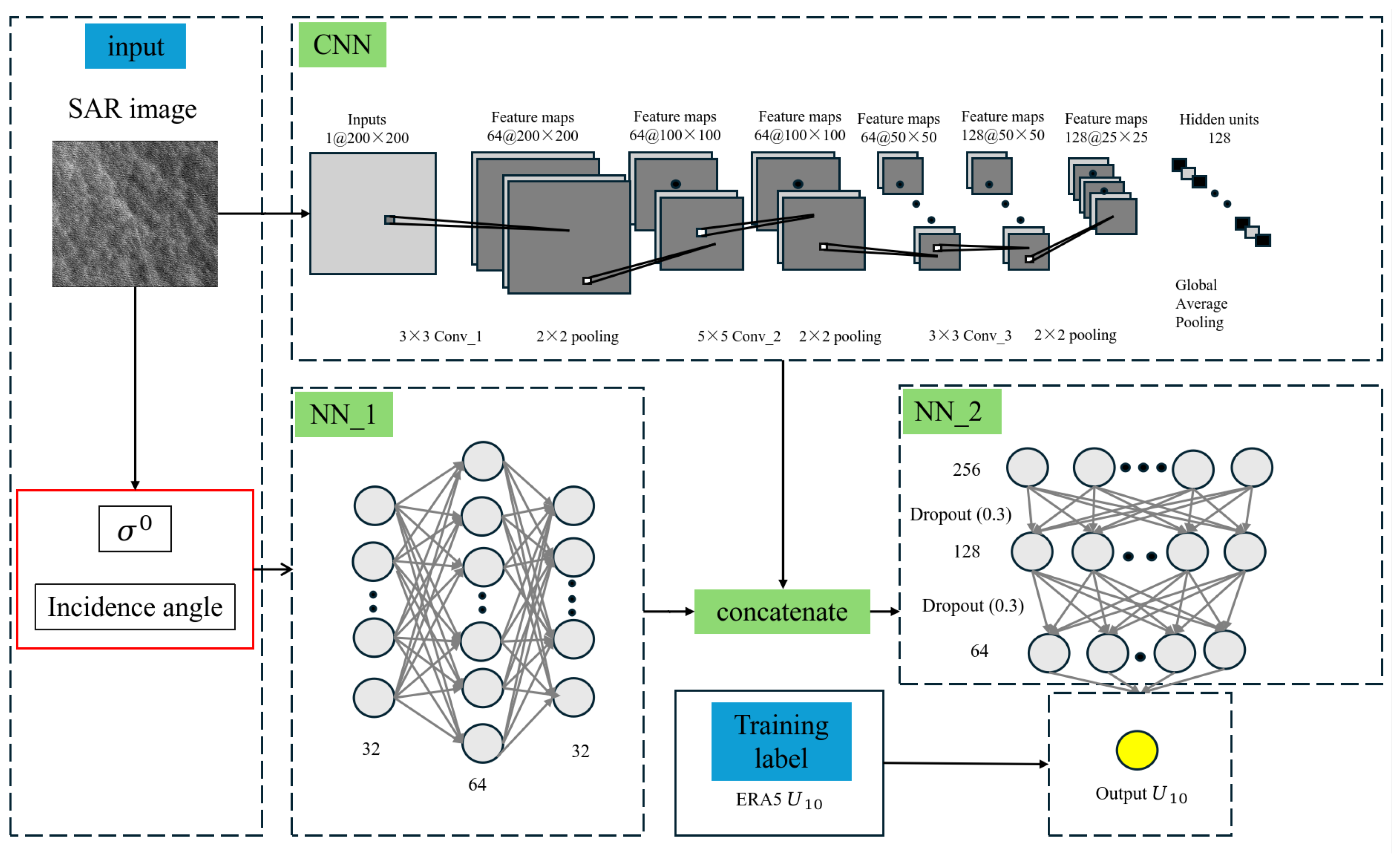
To model the relationship between Sentinel-1 SAR image features, radar backscatter coefficients (${\sigma }^0$), and 10 m wind speed ($U_{10}$), a hybrid deep learning architecture is developed, as illustrated in Figure 2. The model integrates CNN with fully connected neural networks (NNs) to estimate $U_{10}$ from SAR imagery and ancillary data. The input layer is composed of three components: normalized SAR image, corresponding ${\sigma }^0$ values, and radar incidence angles. The output layer represents the collocated ERA5 $U_{10}$, which is used as the training target. The CNN branch processes the SAR imagery through a sequence of convolutional and pooling layers designed to extract multiscale spatial features. Each SAR input is formatted as a single-channel image with spatial dimensions of 200 × 200 pixels. The initial convolutional layer (3 × 3 Conv_1) generates 64 feature maps while retaining spatial resolution (200 × 200), followed by a Rectified Linear Unit (ReLU) activation. A subsequent 2 × 2 max-pooling layer reduces the spatial size to 100 × 100. The second convolutional layer (5 × 5 Conv_2), also with 64 filters and ReLU activation, is followed by another 2 × 2 pooling layer. The third convolutional layer (3 × 3 Conv_3) increases the feature map count to 128, again followed by ReLU and a final 2 × 2 pooling layer that reduces the spatial dimensions to 25 × 25. A global average pooling operation then adds the extracted features into a 128-dimensional vector, which is forwarded to the fully connected component of the network. The radar variables including backscattering coefficient and incidence angle are taken as input the first neural network termed as NN_1 through three hidden layers consisting of 32, 64, and 32 neurons, respectively. Outputs from the CNN and NN_1 branches are concatenated to form a unified feature vector. This combined representation is then input into the second neural network termed as NN_2 through three additional fully connected layers with 256, 128, and 64 neurons. ReLU activation is applied after each layer, with dropout regularization (dropout rate = 0.3) used after the first two layers to mitigate overfitting. The final output layer, without activation, performs a linear regression to predict $U_{10}$.

3. Model Training

3.1. Sensitivity Test

To assess the influence of key hyperparameters on model performance, we conducted a sensitivity analysis focusing on the learning rate and input image size. In the 2017 WV2 dataset, we randomly select 10,000 images and their corresponding data, which are divided into training, validation, and test sets in a 6:2:2 ratio for sensitivity testing. These parameters play a critical role in determining the convergence behavior and predictive accuracy of deep learning models. The Mean Absolute Error (MAE) is employed as the loss function for this network. The model performance is evaluated using the root mean square error (RMSE) between the predicted and reference wind speeds. These two evaluation metrics are defined as follows:

$$MAE={\displaystyle \frac{{\sum }_{i=1}^n\left|f\left(x_i\right)-y_i\right|}{n}}$$

(1)

$$RMSE=\sqrt{{\displaystyle \frac{{\sum }_{i=1}^n{(f\left(x_i\right)-y_i)}^2}{n}}}$$

(2)

where n represents the number of samples, $f\left(x_i\right)$ is the retrieved $U_{10}$ of the i-th sample, and $y_i$ is the actual value of the i-th ERA5 $U_{10}$.

Figure 3a illustrates the sensitivity of model performance to the learning rate. The x-axis represents a logarithmic scale of learning rates, ranging from ${10}^{-6}$ to ${10}^{-2}$, and the y-axis shows the corresponding RMSE. As the learning rate increases, the RMSE initially decreases, reaching a minimum around ${10}^{-4}$, where the model performs optimally with an RMSE of approximately 1.2 m/s. However, as the learning rate continues to rise beyond this point, the model performance degrades with a sharp increase in the RMSE metrics. This indicates that very high learning rates lead to instability in the optimization process, causing the model to fail to converge to the optimal solution. The results suggest that a learning rate in the range of ${10}^{-5}$ to ${10}^{-4}$ offers the best trade-off between convergence speed and model accuracy.

Figure 3b shows the sensitivity of model performance to the image size used during training. The x-axis represents various image sizes, ranging from 400 × 400 pixels to 50 × 50 pixels, while the y-axis again shows the RMSE. The plot reveals that medium image sizes (e.g., 200 × 200) correspond to better model performance, with the RMSE decreasing to around 1.2 m/s for 200 × 200 images. As the image size decreases, the RMSE gradually increases, with the smallest image size (50 × 50) resulting in the highest RMSE of around 1.6 m/s. This trend suggests that using medium image sizes allows the model to capture more detailed spatial information, which improves its ability to accurately retrieve wind speeds. This degradation is likely due to the loss of spatial detail and surface structure, which are essential for accurately characterizing wind-related features in SAR imagery. Together, the results presented in Figure 3 list the importance of tuning hyperparameters to achieve the best model performance. Specifically, a learning rate in the range of ${10}^{-5}$ to ${10}^{-4}$ and 200 × 200 images are employed to minimize RMSE in wind speed retrieval tasks presented in this study.

3.2. Unimodel for Two Incidence Angle

Given the great performance of deep learning in resolving complex task, the first trial is to build a unified inversion model combining both incidence angles from WV1 and WV2 based on the model architecture above. Figure 4a shows the progression of training and validation loss over 150 training epochs. The training loss (blue line) exhibits a continuous decline as the model parameters are iteratively optimized, indicating effective convergence on the training dataset. The validation loss (red line) initially follows a similar dropping trend but begins to oscillate after approximately 50 epochs, suggesting the beginning of overfitting. The epoch corresponding to the minimum validation loss is marked by a vertical black line and defines the optimal model state selected for final evaluation. The persistent gap between training and validation losses in the later epochs highlights a typical trade-off in deep learning, wherein continued training can lead to improved performance on the training set at the expense of generalization to validation data. Despite this, the observed convergence pattern indicates that the model successfully captures the dominant signal in the training data while preserving generalization capacity on the validation set.

Quantitative model performance is further assessed in Figure 4b, which compares predicted 10 m wind speed ($U_{10}$) against collocated ERA5 $U_{10}$ values for the test dataset. The evaluation is based on over 119,000 independent matchups not used during training. The scatter plot reveals a strong linear relationship between predicted and reference wind speeds with evident underestimation at higher wind speeds. The root mean square error (RMSE) is 1.19 m/s, and the mean bias is −0.09 m/s, indicating overall high model accuracy and minimal systematic error. The red dashed line represents the linear regression fit (y = 0.80x + 1.38), while the one-to-one in solid black. The regression slope and positive intercept suggest a conservative bias under high-wind conditions, likely due to the distribution of training samples and the nonlinear response of radar backscatter under strong wind forcing. This behavior is consistent with previously reported saturation effects in C-band SAR measurements at high wind speeds. These findings demonstrate that the integration of WV1 and WV2 datasets within a unified inversion framework yields accurate and consistent surface wind speed retrievals. Model performance, as assessed by standard validation metrics, is comparable to or exceeds that of traditional approaches. The model exhibits stable convergence during training and shows strong agreement with collocated ERA5 wind speeds, indicating its robustness across a range of geophysical conditions.

3.3. Respective Model for Each Incidence

Given the fact that radar backscattering mechanism at the two incidence angles of WV1 and WV2 are slightly different, it is necessary to evaluate the model performance built for each incidence angle. Figure 5 presents the two wind speed inversion models. Figure 5a,b display the training and validation loss curves for the WV1- and WV2-based models over 150 training epochs. The training loss (blue lines) shows a consistent decreasing trend for both models, indicative of effective learning and stable convergence of the optimization process. The validation loss (red lines) initially decreases but exhibits minor fluctuations in later epochs, suggesting the potential overfitting. Vertical black lines denote the epochs at which the minimum validation loss is achieved; these points define the optimal model checkpoints used for subsequent evaluation. Both models demonstrate similar training dynamics; however, the WV2-based model achieves a slightly lower minimum validation loss than the WV1 counterpart, implying potentially stronger generalization to validation data.

Panels (b) and (d) provide a quantitative evaluation of model performance against collocated ERA5 $U_{10}$ for the test dataset not used in training. In Figure 5b, the WV1-trained model yields a RMSE of 1.24 m/s and a mean bias of 0.10 m/s across 58,474 test points. The regression fit, represented by the equation y = 0.81x + 1.47, deviates from the one-to-one line, particularly at wind speeds exceeding 12 m/s. This underestimation at higher wind speeds is consistent with known limitations in SAR wind retrieval. Additional contributing factors may include sampling imbalances in the training set that favor moderate wind speeds. Figure 5d presents the corresponding analysis for the WV2-trained model. This model achieves a lower RMSE of 1.08 m/s and a reduced mean bias of 0.02 m/s over 61,903 samples. The regression equation, y = 0.88x + 0.95, more closely aligns with the one-to-one line, reflecting improved accuracy across the full wind speed range. The enhanced performance may result from differences in radar incidence angle, image acquisition geometry, or geophysical conditions specific to WV2 scenes, which may improve the sensitivity of ${\sigma }^0$ to surface wind variations. Overall, it highlights the distinct retrieval behavior of models trained on WV1 and WV2 datasets independently. While both models demonstrate high retrieval skill, the WV2-based model outperforms in terms of both accuracy and bia. These results emphasize the need of tailoring machine learning-based inversion to specific SAR imaging modes of WV1 and WV2 observations.

4. Results Validation

4.1. Independent Validation with ERA5 Wind Speed

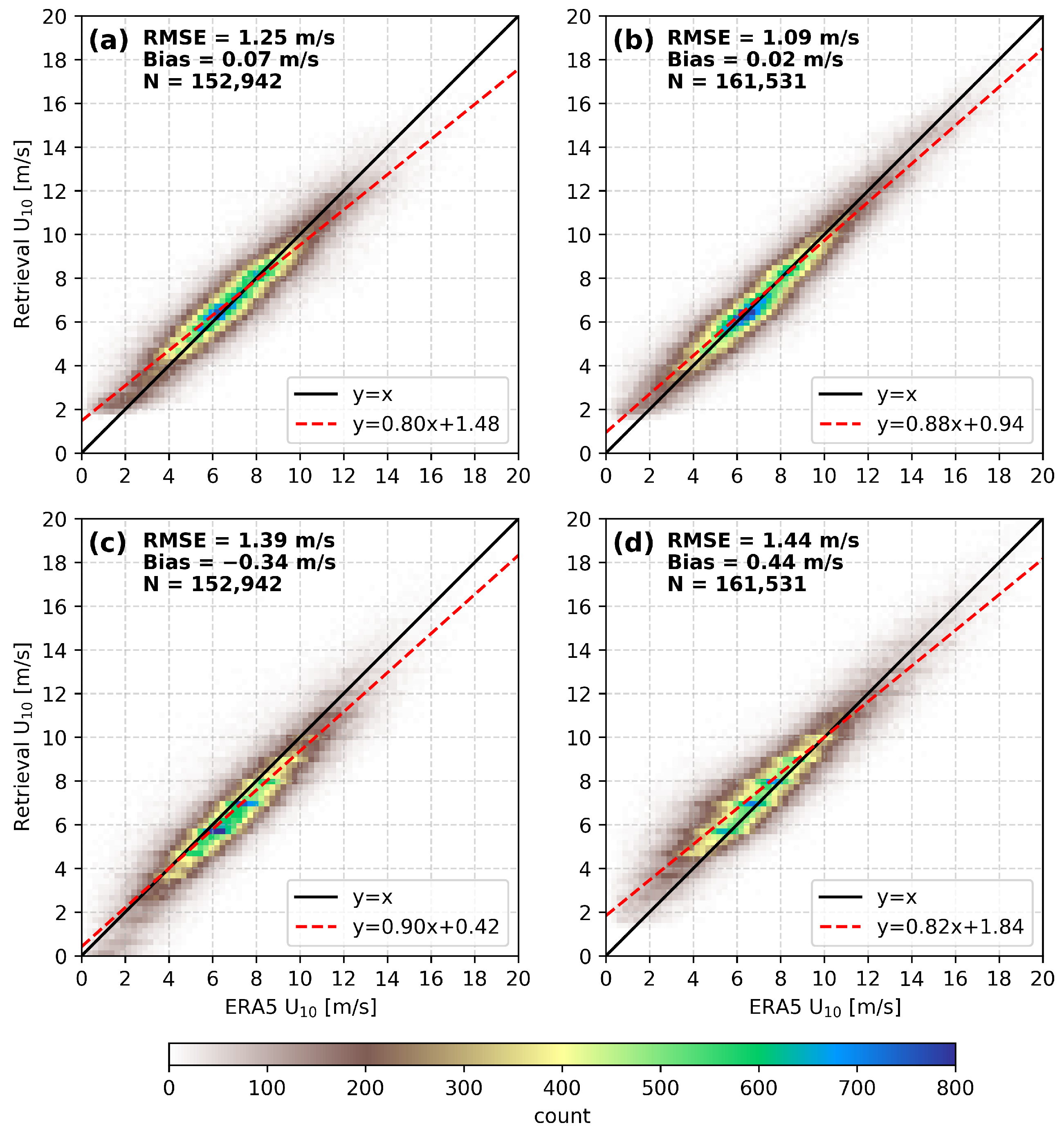
To independently assess the performance of the CNN-based inversion models developed for each incidence angle, a validation experiment is conducted using Sentinel-1 wave mode data acquired from July to December 2016. This evaluation compares wind speed retrievals from the CNN models trained on WV1 and WV2 data with those obtained from the GMF-based algorithm CMOD5.N. All retrievals are validated against collocated ERA5 reanalysis $U_{10}$ values. Figure 6 presents a summary of the results. Panels (a) and (b) show scatter plots of CNN-retrieved $U_{10}$ versus ERA5 reference values for WV1 and WV2, respectively. Both models exhibit a tight clustering of points around the one-to-one line (black solid line), particularly in the 4–12 m/s wind speed range, indicating strong agreement with ERA5. The RMSE is 1.25 m/s for the WV1 model and 1.09 m/s for WV2, with corresponding biases of 0.07 m/s and 0.02 m/s. These metrics confirm the high accuracy and minimal systematic error of the CNN approach, with WV2-based retrievals showing enhanced performance. The red dashed lines represent linear regression fits to the data, with slopes of 0.80 (WV1) and 0.88 (WV2), indicating slight underestimation at higher wind speeds—a known limitation in SAR wind retrieval.

Panels (c) and (d) of Figure 6 display the corresponding results using the CMOD5.N algorithm, driven by ERA5 wind direction as an external input. This traditional GMF-based method yields RMSE values of 1.39 m/s (WV1) and 1.44 m/s (WV2), with biases of −0.34 m/s and 0.44 m/s, respectively. Compared to the CNN models, the CMOD5.N retrievals show larger errors and greater deviations from the one-to-one line. In particular, the WV2-based CMOD5.N result (Figure 6d) exhibits overestimation at lower wind speeds, reflected in a flatter regression slope of 0.82 and a higher intercept of 1.84 m/s. The increased scatter and wider distribution, especially at wind speed extremes, suggest reduced robustness of the GMF-based method under varying oceanic conditions. While a positive correlation with the reference is maintained, the dispersion of points away from the ideal agreement line is more pronounced than that observed in the CNN-based retrievals. In addition, the most significant improvements in performance over traditional algorithms are observed in the low-to-moderate wind speed regime (4–12 m/s), where the CNN model demonstrates a marked reduction in both RMSE and systematic bias, highlighting its enhanced ability to interpret complex sea surface textures in these common conditions.

4.2. Comparison with Buoys

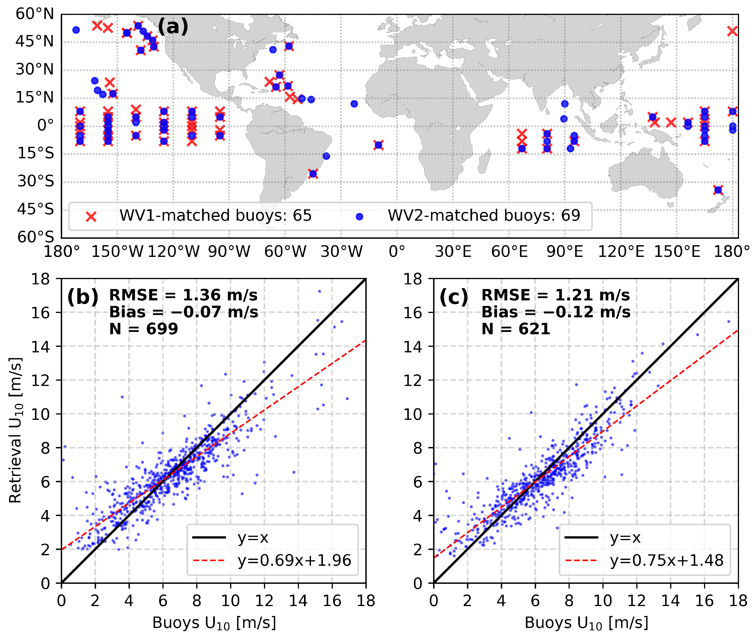
To further evaluate the performance of the proposed CNN-based inversion model for surface wind retrieval, validation against independent in situ measurements is essential. In this analysis, collocated comparisons are conducted between model-retrieved 10 m wind speeds ($U_{10}$) and observations from buoys. Figure 7 presents the validation results versus the collocated buoy measurements. Figure 7a shows the geographic distribution of buoys that are spatiotemporally matched with S-1 SAR acquisitions during 2016. Matches with WV1 and WV2 data are indicated by red crosses and blue circles, respectively. A total of 65 buoys are matched with WV1 images and 69 with WV2, covering a broad geographic domain across multiple ocean basins. This extensive spatial coverage ensures a representative sampling of diverse environmental regimes, including both tropical and mid-latitude regions, which is critical for validating model robustness under varying oceanographic and atmospheric conditions.

The lower panels of Figure 7 provide scatter plots comparing the CNN-retrieved $U_{10}$ values with collocated buoy measurements. The solid black line denotes the one-to-one reference line, while the red dashed line represents the least-squares linear regression fit, accompanied by the regression equation and key performance metrics. In Figure 7b, validation using WV1-based retrievals yields a RMSE of 1.36 m/s and a mean bias of −0.07 m/s based on 699 matchups. The regression line has a slope of 0.69 and an intercept of 1.96 m/s, indicating that the model reproduces the overall wind speed trend but tends to overestimate at lower wind speeds and underrepresent variability at higher wind speeds. Figure 7c presents the validation results for the CNN model trained on WV2 data. This configuration yields improved performance, with an RMSE of 1.21 m/s and a reduced bias of −0.12 m/s across 621 collocated samples. The regression slope increases to 0.75 and the intercept decreases to 1.48 m/s, indicating a closer alignment with buoy-observed wind speeds and a more accurate representation of wind variability. The improved accuracy of the WV2-based retrievals may be attributed to the enhanced sensitivity to surface wind signatures in SAR backscatter at larger incidence angle. Overall, these validation results reinforce the capability of the CNN-based inversion approach to retrieve ocean surface wind speeds with reasonable accuracy when compared against in situ observations. It is also important to acknowledge the limitations of the buoy validation dataset. While providing a crucial ground truth, the 699 matchups represent a much smaller sample size than the ERA5 data used for large-scale validation. Critically, the dataset is sparse in the high wind speed regime, with only a few dozen matchups where buoy-measured winds exceed 12 m/s. Such a lack of high-wind events may influence the performance metrics. The observed underestimation at higher wind speeds could therefore be, in part, a statistical artifact of this sampling bias rather than a fundamental limitation of the model predictive capability in these conditions. A more robust assessment of high-wind performance would require a larger, more representative dataset of in situ measurements.

4.3. Performance Diagnostics

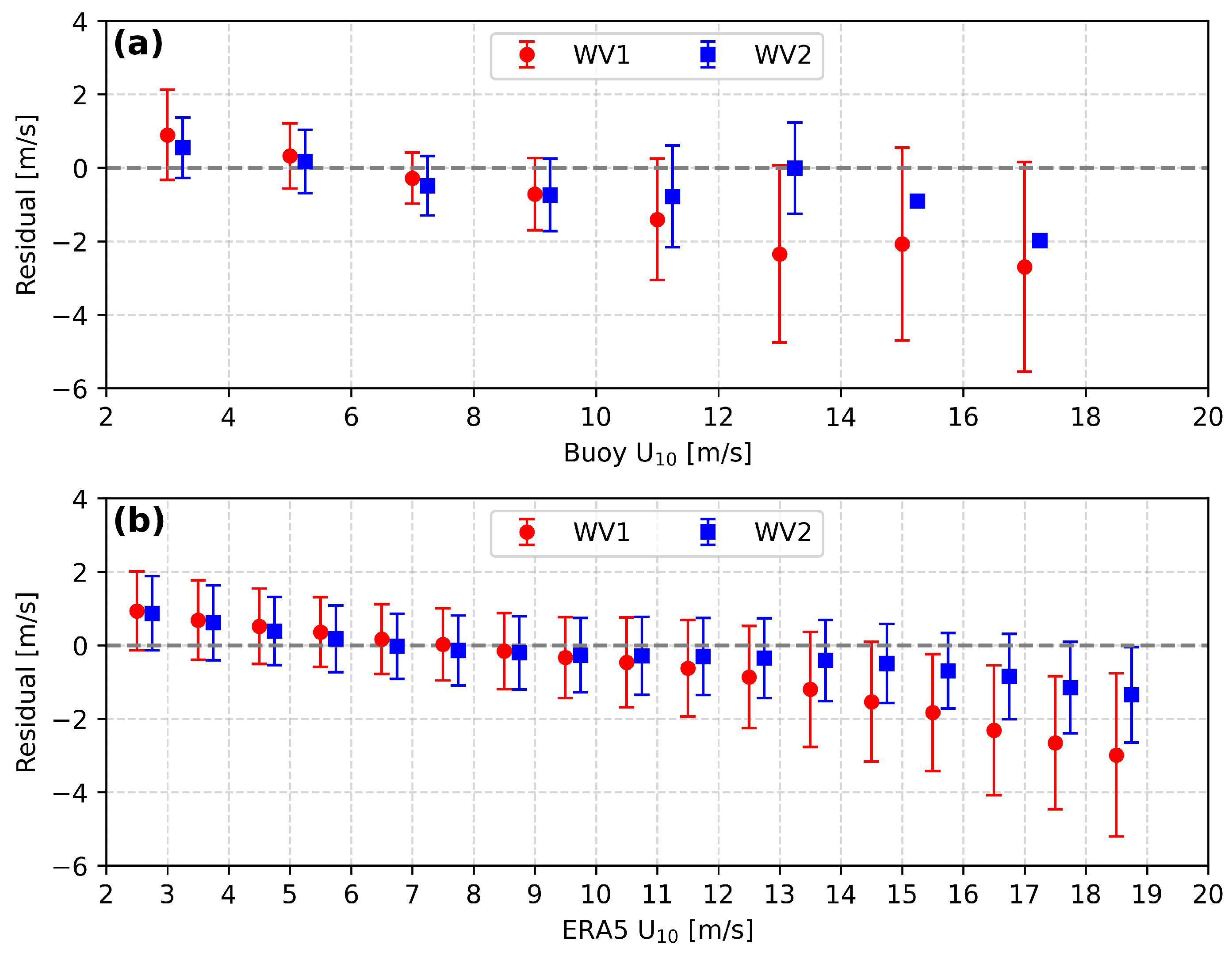
To comprehensively assess the retrieval accuracy and robustness of the proposed CNN-based inversion models, a series of diagnostic evaluations are conducted. These include analysis of residual error distributions, examination of systematic bias trends, and assessment of regional variability in model performance. Validation is carried out separately across different wind speed regimes and SAR image acquisition categories to evaluate retrieval stability under varying geophysical conditions. Figure 8 provides a detailed view of wind speed residuals defined as the difference between the CNN-retrieved and reference $U_{10}$ versus the reference wind speed. This approach facilitates the identification of systematic errors and the quantification of retrieval uncertainty across a range of wind conditions, supplementing the overall metrics presented in Figure 6 and Figure 7. Panel (a) compares CNN retrievals with in situ buoy observations, while panel (b) uses ERA5 reanalysis data as the reference. Results for WV1 and WV2 retrievals are represented by red circles and blue squares, respectively. Each marker corresponds to the mean residual within 1 m/s bins of reference wind speed, with error bars indicating one standard deviation.

In Figure 8a, residuals are plotted against buoy-measured $U_{10}$, spanning reference wind speeds from approximately 3 to 17 m/s. At lower wind speeds (<6 m/s), both WV1 and WV2 retrievals show positive residuals, indicating a systematic overestimation of wind speed under calm conditions. This effect is more pronounced for WV2, where mean residuals exceed 2 m/s in bins centered at 4–5 m/s. As wind speed increases, residuals for both modes approach zero, although variability also increases. At higher wind speeds (>10 m/s), WV1 retrievals exhibit a consistent negative bias, reaching approximately −2 m/s in the uppermost bins, suggesting underestimation in strong wind regimes. WV2 retrievals follow a similar pattern but with smaller amplitude and lower variance, indicating improved retrieval stability across the full wind spectrum. Panel (b) presents the residuals with respect to ERA5 $U_{10}$, which serves as the training target for the CNN models. Compared to the buoy-based validation, residuals here are generally smaller in magnitude and exhibit more consistent trends across all wind speed bins. For low-to-moderate wind speeds (3–9 m/s), WV1 residuals remain slightly positive, ranging from 0.5 to 1.5 m/s, while WV2 residuals are closer to zero. At higher wind speeds (>14 m/s), both retrievals exhibit a modest negative bias, although the magnitude remains less than that observed in the buoy comparison. The reduced variance in ERA5-based residuals, particularly for WV2, suggests strong alignment between the CNN output and the training data distribution. However, the broader spread observed in WV1 residuals at the upper wind range may reflect limitations in training sample representation or diminished SAR image quality under extreme conditions.

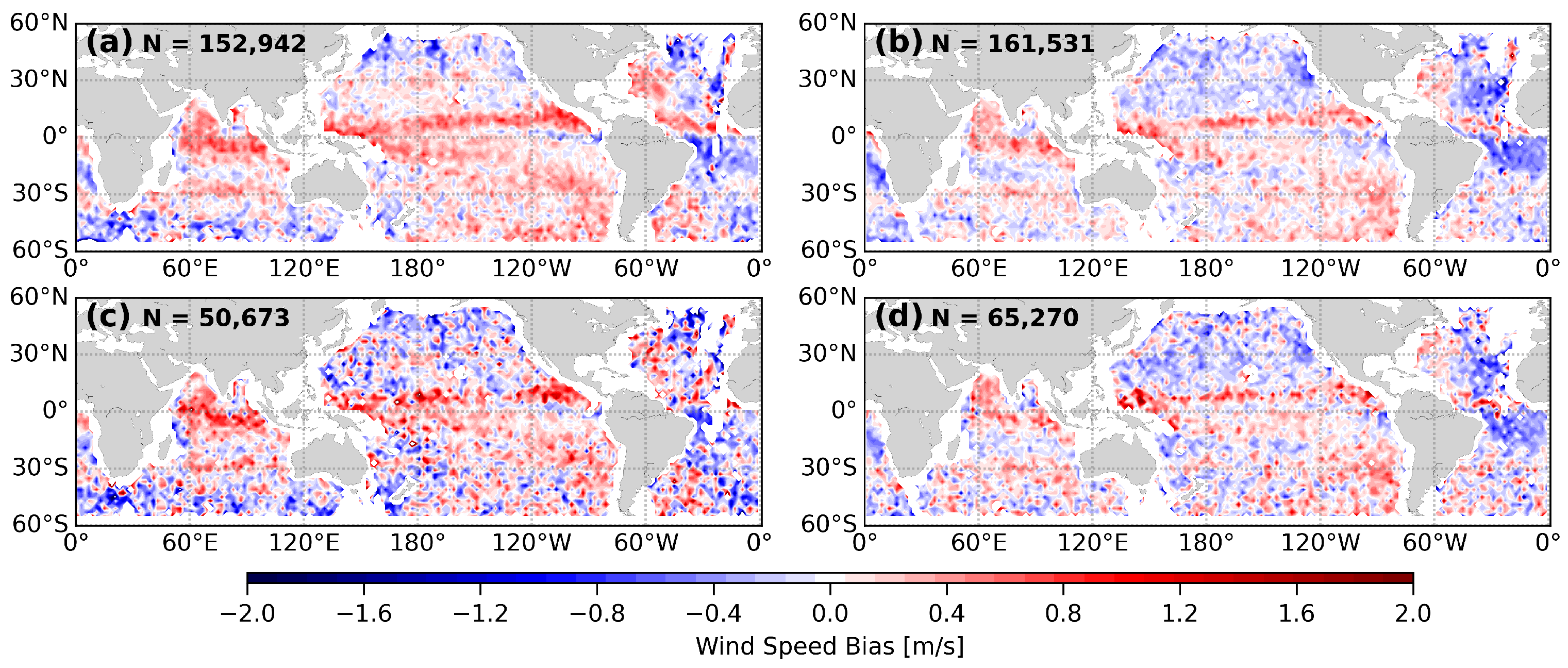
Figure 9 illustrates the global distribution of wind speed bias, defined as the mean difference between SAR-retrieved and reference wind speeds (retrieval–reference), gridded at a spatial resolution of 2° × 2°. Panels (a) and (b) show the bias fields derived from all available WV images for WV1 and WV2 acquisitions, respectively. Panels (c) and (d) depict results from a subset of scenes classified by dominant ocean surface features—specifically, pure ocean swell, wind streaks, and convective cells—based on a CNN-based scene classification method documented in [30].

In the analysis based on all SAR images (panels a and b), distinct spatial patterns emerge between the two acquisition modes. WV1-based retrievals (Figure 9a) exhibit pronounced positive biases, reaching up to 2 m/s, particularly across equatorial and tropical latitudes, including the central and western Pacific and portions of the Indian Ocean. These overestimations are consistent with prior observations, suggesting that swell-dominated surface roughness in low-wind regimes can enhance radar backscatter, leading to enhanced wind speed estimates. Negative biases ranging from −1 to −2 m/s are scattered but are more frequent at higher latitudes in both hemispheres, including the mid-latitude North Pacific and the Southern Ocean. These regions are often characterized by rapidly evolving atmospheric conditions or high wind events, where retrieval uncertainty increases due to nonlinearities in the backscatter response. In contrast, WV2 retrievals in Figure 9b show reduced bias magnitudes and a more balanced spatial distribution of over- and underestimation. This relative improvement may be attributed to the larger incidence angles of WV2, which enhances sensitivity to surface wind variability. However, regional pockets of significant bias persist, especially over the western Pacific and Indian Ocean, suggesting that localized environmental factors or acquisition parameters continue to influence retrieval performance. The residual plot in Figure 8 reveals two systematic trends: a slight overestimation at low wind speeds (<4 m/s) and a more pronounced underestimation at high wind speeds (>12 m/s). These biases likely have physical origins. The overestimation at low wind speeds is potentially linked to the influence of ocean swell. Under low-wind conditions, swell-generated roughness can increase SAR backscatter, which the model may misinterpret as wind, leading to an overestimation. This hypothesis is supported by the spatial bias maps (Figure 9), where positive biases are often observed in regions known for persistent swell. Similarly, the underestimation at high wind speeds is linked to signal saturation and reduced sensitivity of the SAR cross section under high-wind conditions, as reflected in the negative bias patterns in high-latitude and convective regions.

In Figure 9c, WV1 retrievals from classified scenes reveal that positive wind speed biases are more spatially constrained and largely aligned with equatorial swell zones, supporting the hypothesis that surface wave modulation contributes to backscatter enhancement. Negative biases dominate in higher-latitude regions, particularly those associated with cyclonic systems or convective activity, where atmospheric variability may impact SAR image quality and retrieval accuracy. The total number of classified WV1 scenes (N = 50,673) is substantially smaller than the full dataset, reflecting the lower frequency of these surface type assignments at the global scale. In Figure 9d, the WV2 subset exhibits similar spatial bias patterns, but with broader geographic coverage and increased spatial continuity. Areas of larger positive bias are evident in the western Pacific warm pool and Indian Ocean, consistent with the prevalence of wind streaks and convective features in these regions. The contrast between the full and classified analyses emphasize the influence of underlying surface processes on SAR wind retrieval accuracy. These results highlight the importance of accounting for surface feature variability when interpreting SAR-derived wind fields, particularly in regions where sea surface conditions deviate from the assumptions inherent in geophysical model functions.

5. Summary

In this study, a CNN-based framework was developed for retrieving ocean surface wind speed from S-1 SAR wave mode observations. The model is trained on observations from 2017 using ERA5 reanalysis wind vectors as reference and validated with independent S-1 acquisitions from 2016, as well as collocated in situ measurements. Evaluation results indicate that the CNN model achieves high retrieval accuracy across both incidence angle modes (WV1 and WV2), with strong consistency against both ERA5 and buoy-derived $U_{10}$. When compared against the conventional CMOD5.N-based results, the CNN approach demonstrates significant reductions in RMSE and mean bias, particularly within the low-to-moderate wind speed regime. The model further exhibits effective generalization when applied to datasets excluded from the training phase, supporting its robustness. A sensitivity analysis revealed that model performance is influenced by hyperparameters, with optimal results achieved using a learning rate of 10⁻⁵ and input image size of 200 × 200 pixels. Residual diagnostics indicate a tendency for the model to overestimate wind speeds under low-wind conditions and to slightly underestimate high-wind events. These systematic deviations, although modest, highlight opportunities for further refinement through bias correction techniques or incorporation of physically informed constraints during training. Spatial bias maps revealed geographic variability in model performance, influenced by sea surface state and environmental conditions. Through SAR scene classification into dominant surface types (e.g., swell, wind streaks, convective cells), the analysis demonstrates that retrieval bias is modulated by underlying surface features. WV2-based retrievals exhibited lower bias and improved spatial consistency relative to WV1, likely due to acquisition geometry and incidence angle differences.

Despite these encouraging results, several limitations remain. First, the use of ERA5 reanalysis as the reference dataset introduces uncertainty due to model and assimilation errors inherent in the reanalysis framework. Future research should evaluate model performance against higher-accuracy references, such as scatterometer observations or dual-frequency buoy systems, to further validate retrieval accuracy. Second, the current framework is fully data-driven and does not incorporate physical priors. Integrating physical constraints or developing hybrid physics-informed neural networks may enhance both predictive performance and interpretability. Limitations also arise from the choice of input image resolution and network depth. The use of 200 × 200 pixel image patches may limit the model ability to resolve fine-scale wind features associated with mesoscale atmospheric dynamics or submesoscale ocean processes. In addition, the relatively shallow CNN architecture, designed to ensure training stability and reduce computational cost, may constrain the network ability to extract multiscale spatial features. More advanced architectures, such as those incorporating residual blocks or attention mechanisms, could enhance model capacity, though such modifications would require careful regularization to prevent overfitting, especially under limited training data scenarios. Finally, while the CNN model demonstrated strong generalization across typical oceanic conditions, its performance under extreme weather system, such as tropical cyclones or polar lows, remains to be evaluated and may represent an important direction for future investigation. In addition, while the current study focuses on the validation of our retrieval methodology, we recognize the potential for applying this model to conduct detailed climatological analyses. Investigating the seasonal and diurnal distributions of wind speed using our validated model would be a significant contribution and represents a promising avenue for future research.

The proposed CNN-based retrieval framework provides a foundation for broader applications in satellite-based ocean surface wind estimation. A key advantage of the method is its ability to retrieve wind speed without requiring auxiliary wind direction input, a limitation inherent to GMF-based algorithms. This not only simplifies the inversion process but also creates the possibility of reversing the traditional workflow: accurate wind speed retrievals can be used to infer wind direction, potentially through analysis of SAR-derived wind streak orientation or wave alignment features. Additionally, the retrieved wind fields may support secondary products, such as significant wave height, especially in scenarios where directional ambiguity or lack of supporting wave model data limits traditional approaches. Coupling CNN-based wind retrievals with wave information from SAR or external sources could enable a fully data-driven framework for joint estimation of surface wind, direction, and sea state parameters. This integrated approach has the potential to advance understanding of air–sea interaction processes, including momentum transfer, boundary layer dynamics, and wave–wind coupling. Future development may include multi-task learning or coupled neural architectures to jointly retrieve wind and wave parameters from SAR data. Such advancements would be particularly valuable in operational marine forecasting systems and climate-scale diagnostics, offering a more comprehensive view of ocean–atmosphere exchange processes.

References

1. Smith, S.D. Coefficients for sea surface wind stress, heat flux, and wind profiles as a function of wind speed and temperature. J. Geophys. Res. Ocean. 1988, 93, 15467–15472. [Google Scholar] [CrossRef]
2. Yu, L. Global air–sea fluxes of heat, fresh water, and momentum: Energy budget closure and unanswered questions. Annu. Rev. Mar. Sci. 2019, 11, 227–248. [Google Scholar] [CrossRef]
3. Cronin, M.F.; Gentemann, C.L.; Edson, J.; Ueki, I.; Bourassa, M.; Brown, S.; Clayson, C.A.; Fairall, C.W.; Farrar, J.T.; Gille, S.T.; et al. Air-sea fluxes with a focus on heat and momentum. Front. Mar. Sci. 2019, 6, 430. [Google Scholar] [CrossRef]
4. Villas Bôas, A.B.; Ardhuin, F.; Ayet, A.; Bourassa, M.A.; Brandt, P.; Chapron, B.; Cornuelle, B.D.; Farrar, J.T.; Fewings, M.R.; Fox-Kemper, B.; et al. Integrated observations of global surface winds, currents, and waves: Requirements and challenges for the next decade. Front. Mar. Sci. 2019, 6, 434339. [Google Scholar] [CrossRef]
5. Hong, B.; Zhang, J. Long-term trends of sea surface wind in the northern South China Sea under the background of climate change. J. Mar. Sci. Eng. 2021, 9, 752. [Google Scholar] [CrossRef]
6. Bourassa, M.A.; Meissner, T.; Cerovecki, I.; Chang, P.S.; Dong, X.; De Chiara, G.; Donlon, C.; Dukhovskoy, D.S.; Elya, J.; Fore, A.; et al. Remotely sensed winds and wind stresses for marine forecasting and ocean modeling. Front. Mar. Sci. 2019, 6, 443. [Google Scholar] [CrossRef]
7. Sempreviva, A.M.; Barthelmie, R.J.; Pryor, S. Review of methodologies for offshore wind resource assessment in European seas. Surv. Geophys. 2008, 29, 471–497. [Google Scholar] [CrossRef]
8. Doubrawa, P.; Barthelmie, R.J.; Pryor, S.C.; Hasager, C.B.; Badger, M.; Karagali, I. Satellite winds as a tool for offshore wind resource assessment: The Great Lakes Wind Atlas. Remote Sens. Environ. 2015, 168, 349–359. [Google Scholar] [CrossRef]
9. Ricciardulli, L.; Manaster, A.; Lindsley, R. Investigation of a calibration change in the ocean surface wind measurements from the TAO buoy array. Bull. Am. Meteorol. Soc. 2025, 106, E242–E260. [Google Scholar] [CrossRef]
10. Yueh, S.H.; Dinardo, S.J.; Fore, A.G.; Li, F.K. Passive and active L-band microwave observations and modeling of ocean surface winds. IEEE Trans. Geosci. Remote Sens. 2010, 48, 3087–3100. [Google Scholar] [CrossRef]
11. Klemas, V. Remote sensing techniques for studying coastal ecosystems: An overview. J. Coast. Res. 2011, 27, 2–17. [Google Scholar]
12. Chelton, D.B.; Schlax, M.G.; Freilich, M.H.; Milliff, R.F. Satellite Measurements Reveal Persistent Small-Scale Features in Ocean Winds. Science 2004, 303, 978–983. [Google Scholar] [CrossRef]
13. O’Neill, L.W.; Chelton, D.B.; Esbensen, S.K. Covariability of Surface Wind and Stress Responses to Sea Surface Temperature Fronts. J. Clim. 2012, 25, 5916–5942. [Google Scholar] [CrossRef]
14. Figa-Saldaña, J.; Wilson, J.J.; Gelsthorpe, R.; Stoffelen, A. The advanced scatterometer (ASCAT) on the meteorological operational (MetOp) platform: A follow on for European wind scatterometers. Can. J. Remote Sens. 2002, 28, 404–412. [Google Scholar] [CrossRef]
15. Sun, J.; Li, H.; Lin, W.; He, Y. Joint inversion of sea surface wind and current velocity based on Sentinel-1 synthetic aperture radar observations. J. Mar. Sci. Eng. 2024, 12, 450. [Google Scholar] [CrossRef]
16. Montuori, A.; Portabella, M.; Guimbard, S.; Gabarró, C.; Migliaccio, M. Assessment of the SMOS inversion scheme for salinity and wind speed retrieval purposes. Eur. J. Remote Sens. 2013, 46, 855–873. [Google Scholar] [CrossRef]
17. Mourad, P.D.; Thompson, D.R.; Vandemark, D.C. Extracting fine-scale wind fields from synthetic aperture radar images of the ocean surface. Johns Hopkins APL Tech. Dig. 2000, 21, 108–115. [Google Scholar]
18. Lin, H.; Xu, Q.; Zheng, Q. An overview on SAR measurements of sea surface wind. Prog. Nat. Sci. 2008, 18, 913–919. [Google Scholar] [CrossRef]
19. Wang, C.; Vandemark, D.; Mouche, A.; Chapron, B.; Li, H.; Foster, R.C. An assessment of marine atmospheric boundary layer roll detection using Sentinel-1 SAR data. Remote Sens. Environ. 2020, 250, 112031. [Google Scholar] [CrossRef]
20. Mouche, A.A.; Collard, F.; Chapron, B.; Dagestad, K.F.; Guitton, G.; Johannessen, J.A.; Kerbaol, V.; Hansen, M.W. On the use of Doppler shift for sea surface wind retrieval from SAR. IEEE Trans. Geosci. Remote Sens. 2012, 50, 2901–2909. [Google Scholar] [CrossRef]
21. Li, H.; Chapron, B.; Mouche, A.; Wang, C.; Lin, W.; He, Y. Ocean Surface Wind Wave Signatures in Single-Look Complex SAR Data. IEEE Trans. Geosci. Remote Sens. 2025, 63, 4203111. [Google Scholar] [CrossRef]
22. Yu, P.; Xu, W.; Zhong, X.; Johannessen, J.A.; Yan, X.H.; Geng, X.; He, Y.; Lu, W. A neural network method for retrieving sea surface wind speed for C-Band SAR. Remote Sens. 2022, 14, 2269. [Google Scholar] [CrossRef]
23. Li, X.M. Retrieval of Sea Surface Wind Speed by Spaceborne SAR Based on Machine Learning. In Proceedings of the IGARSS 2020–2020 IEEE International Geoscience and Remote Sensing Symposium, Waikoloa, HI, USA, 26 September–2 October 2020; pp. 4011–4014. [Google Scholar]
24. Zanchetta, A.; Zecchetto, S. Wind direction retrieval from Sentinel-1 SAR images using ResNet. Remote Sens. Environ. 2021, 253, 112178. [Google Scholar] [CrossRef]
25. Li, H.; Mouche, A.; Stopa, J.E. Impact of sea state on wind retrieval from Sentinel-1 wave mode data. IEEE J. Sel. Top. Appl. Earth Obs. Remote Sens. 2019, 12, 559–566. [Google Scholar] [CrossRef]
26. Eyre, J.R.; English, S.J.; Forsythe, M. Assimilation of satellite data in numerical weather prediction. Part I: The early years. Q. J. R. Meteorol. Soc. 2020, 146, 49–68. [Google Scholar] [CrossRef]
27. Ramon, J.; Lledó, L.; Torralba, V.; Soret, A.; Doblas-Reyes, F.J. What global reanalysis best represents near-surface winds? Q. J. R. Meteorol. Soc. 2019, 145, 3236–3251. [Google Scholar] [CrossRef]
28. Wang, C.; Mouche, A.; Tandeo, P.; Stopa, J.E.; Longépé, N.; Erhard, G.; Foster, R.C.; Vandemark, D.; Chapron, B. A labelled ocean SAR imagery dataset of ten geophysical phenomena from Sentinel-1 wave mode. Geosci. Data J. 2019, 6, 105–115. [Google Scholar] [CrossRef]
29. Young, I.R. Seasonal variability of the global ocean wind and wave climate. Int. J. Climatol. A J. R. Meteorol. Soc. 1999, 19, 931–950. [Google Scholar] [CrossRef]
30. Wang, C.; Tandeo, P.; Mouche, A.; Stopa, J.E.; Gressani, V.; Longepe, N.; Vandemark, D.; Foster, R.C.; Chapron, B. Classification of the global Sentinel-1 SAR vignettes for ocean surface process studies. Remote Sens. Environ. 2019, 234, 111457. [Google Scholar] [CrossRef]
Figure 1. Monthly count of SAR images included in this study at two incidence angles of (a) WV1 and (b) WV2 between July 2016 and December 2017. Spatial data density at grid of 2° × 2° is given for (c) WV1 and (d) WV2. PDF of collocated ERA5 wind speed for (e) WV1 and (f) WV2 at a bin size of 0.5 m/s.
Jmse 13 01751 g001
Figure 2. Schematic diagram of the neural network architecture used in this study. The input layer consists of the normalized SAR images, the radar backscattering and the radar incidence angle. The output layer corresponds to the collocated wind speed, with inputs consisting of the image, the corresponding σ 0 , and the incidence angle.
Jmse 13 01751 g002
Figure 3. Sensitivity analysis of the model performance versus the hyperparameters of (a) learning rate and (b) image size.
Jmse 13 01751 g003
Figure 4. Performance of a united wind speed inversion combining both WV1 and WV2 for (a) loss variation versus the training epochs. The vertical solid curve indicates the epoch corresponding to the minimum loss metrics. (b) comparison of retrieved wind speed versus the reference based on the test dataset that is not involved in the training. The solid black curve denotes the one-to-one line and the red dashed is the linear regression curve with the error metrics annotated in each plot.
Jmse 13 01751 g004
Figure 5. Performance of wind speed inversion using (a) WV1 and (c) WV2 for loss variation versus the training epochs. The vertical solid curve indicates the epoch corresponding to the minimum loss metrics. Comparison of retrieved wind speed versus the reference based on the test datasets not involved in training: (b) WV1 and (d) WV2. The solid black curve denotes the one-to-one line and the red dashed is the linear regression curve with the error metrics annotated in each plot.
Jmse 13 01751 g005
Figure 6. Independent validation of retrieved wind speed based on SAR images acquired in 2016. (Top) Comparison of wind speed inversed by the CNN model proposed in this work for (a) WV1 and (b) WV2. (Bottom) Scatter plot of wind speed inversion using the traditional GMF-based algorithm by CMOD5.N for (c) WV1 and (d) WV2 with the external wind direction from ERA5. The solid black curve denotes the one-to-one line and the red dashed is the linear regression curve with the error metrics annotated in each plot. The background color shades are the data count binned at 0.25 m/s for both abscissa and ordinate.
Jmse 13 01751 g006
Figure 7. Independent evaluation of wind speed inversion relative to the in situ buoy observations using the dataset in 2016. (a) Spatial locations of collocated buoys for WV1 and WV2. Comparison of model inversed wind speed versus the buoy measurements for (b) WV1 and (c) WV2. The solid black curve denotes the one-to-one line and the red dashed is the linear regression curve with the error metrics annotated in each plot.
Jmse 13 01751 g007
Figure 8. Wind speed difference (retrieval–reference) variation relative to the reference wind speed for (a) buoy measurement and (b) ERA5. Scatters denote the mean difference at wind speed bin of 1 m/s and the error bar denotes one standard deviation.
Jmse 13 01751 g008
Figure 9. Global distribution of the wind speed difference (retrieval–reference) at grid of 2° × 2° for (a) WV1 and (b) WV2 based on all SAR images. The spatial map of wind speed difference for the subset SAR images labeled as pure ocean swell, wind streaks, and convective cells by the classification model: (c) WV1, (d) WV2.
Jmse 13 01751 g009
Disclaimer/Publisher’s Note: The statements, opinions and data contained in all publications are solely those of the individual author(s) and contributor(s) and not of MDPI and/or the editor(s). MDPI and/or the editor(s) disclaim responsibility for any injury to people or property resulting from any ideas, methods, instructions or products referred to in the content.