Spatiotemporal Evolution and Multi-Driver Dynamics of Sea-Level Changes in the Yellow–Bohai Seas (1993–2023)

Abstract

This study analyzes sea-level changes in the Yellow and Bohai Seas from 1993 to 2023 based on satellite altimetry data. After reconstructing the gridded sea-level data using local mean decomposition (LMD), the annual mean sea level was estimated at 28.86 mm, with an average rise rate of 2.21 mm per year (mm/a). Temporal and spatial variations were examined through nonlinear least squares fitting to capture interannual variability and decadal amplitude distributions. Empirical orthogonal function (EOF) analysis identified the first three modes, explaining 90.40%, 2.78%, and 1.47% of the total variance, respectively, and their spatial patterns and temporal coefficients were derived. The first mode was strongly correlated with sea surface temperature (SST) and precipitation, showing distinct spatial structures. Temperature and salinity profiles revealed a decadal-scale trend of increasing temperature and decreasing salinity with depth. Seasonal variations of sea-level anomaly (SLA) were evident, with mean values and trends of −11.47 mm (2.19 mm/a) in spring, 57.12 mm (2.29 mm/a) in summer, 75.68 mm (2.24 mm/a) in autumn, and −13.90 mm (2.11 mm/a) in winter. Seasonal correlations among SLA, SST, salinity, and precipitation were assessed, highlighting interannual amplitude variations. This integrated analysis provides a comprehensive understanding of the dynamics and drivers of sea-level fluctuations, offering insights for future research.

1. Introduction

The Yellow Sea (YS) and Bohai Sea (BS) are shallow, semi-enclosed seas in East Asia, bordered by China and the Korean Peninsula (Figure 1). These seas play a vital role in regional climate regulation, marine ecosystems, and economic activities such as shipping, fishing, and oil extraction [1,2,3]. Given the shallow depths of the Yellow Sea and Bohai Sea, typically ranging from 10 to 50 m, and their proximity to densely populated coastal areas, understanding sea-level changes is critical for managing risks associated with rising sea levels and protecting coastal infrastructure.

Research on sea-level variations in the YS and BS typically relies on satellite altimetry, tide gauge data, and regional ocean models. Satellite altimetry provides long-term trends, tide gauges offer local observations, and ocean models simulate the effects of climatic and hydrological factors [4,5]. Many studies focus on short-term fluctuations or global trends, often overlooking region-specific dynamics crucial for understanding local sea-level changes. Despite the use of satellite altimetry, tide gauge data, and regional models, research on sea-level variability in the YS and BS is limited by the lack of long-term, high-resolution datasets and integrated models that account for local factors like tide-induced variability, coastal subsidence, and regional ocean circulation [6,7,8].

Recent research has focused on advanced signal decomposition techniques, such as empirical mode decomposition (EMD), variational mode decomposition (VMD), and ensemble empirical mode decomposition (EEMD), to improve sea-level estimation accuracy. Local mean decomposition (LMD), derived from EMD, has shown promise in better handling complex, non-stationary signals. For instance, EMD has been applied to examine tidal amplitude changes and to improve the estimation of nonlinear sea-level trends by combining with singular spectrum analysis (SSA) [9,10]. VMD, EEMD, and long short-term memory (LSTM) models have been used in hybrid prediction systems to forecast sea surface height variations [11]. Additionally, signal decomposition techniques have played a crucial role in understanding the accelerated sea-level rise along the U.S. East Coast and in denoising ocean turbulence data [12,13]. These applications contribute to more precise trend estimations and enhanced coastal and oceanic environmental monitoring. Wei et al. [14] explored the use of LMD in GNSS-IR sea-level estimation, showing that it improves accuracy and stability by decomposing signal-to-noise ratio (SNR) components, especially under loose constraints.

This paper presents a new framework for sea-level research, integrating the LMD method, EOF analysis, correlation analysis, and periodicity analysis with multi-source data. The results offer new insights into sea-level changes in the YS and BS regions, providing a foundation for more accurate predictions and better coastal management.

2. Adopted Datasets

This study uses sea-level anomaly (SLA) data from the SLA Gridded (L4) product, covering January 1993 to December 2023 for the YS and BS. Provided by the Copernicus Marine Environment Monitoring Service (CMEMS) and available at https://data.marine.copernicus.eu/products (accessed on 15 December 2024), the data were derived from satellite altimetry missions, including Sentinel-6A, Sentinel-3A/B, Jason-3, CryoSat-2, SARAL-DP/AltiKa, SWOT-nadir, and HY-2B. The data underwent rigorous quality control, including atmospheric corrections and tidal model adjustments. Additionally, sea surface temperature (SST) data, also provided by CMEMS, were included at 0.25° × 0.25° resolution. SST data can be accessed at https://data.marine.copernicus.eu (accessed on 21 December 2024).

The ERA5 reanalysis dataset from ECMWF offers global hourly estimates of atmospheric, oceanic, and land surface variables from 1950 to present. It includes hourly and monthly precipitation data, essential for studying ocean–atmosphere interactions and climate variability, such as ENSO events. Precipitation data can be accessed at https://cds.climate.copernicus.eu/datasets/reanalysis-era5-single-levels-monthly-means?tab=overview(accessed on 20 January 2025).

The Institute of Atmospheric Physics (IAP) Global Ocean Temperature and Salinity Grid provides monthly data on temperature and salinity with a 0.25° × 0.25° resolution and 41 vertical levels (0–2000 m) from 1940 to present. This dataset integrates in situ observations from CTD, Argo, Botter, Glider, and Weoring, combined with model simulations, and has been used since 1960 to estimate ocean heat content changes. Access to this data is available at http://www.ocean.iap.ac.cn (accessed on 6 February 2025).

The study area spans 117° E to 125° E longitude and 30° N to 41° N latitude, covering the YS and BS, to make it possible to analyze spatial sea-level changes and their drivers in this region.

3. Methods

3.1. Local Mean Decomposition Method

Smith et al. introduced local mean decomposition (LMD), an adaptive signal processing method based on empirical mode decomposition (EMD). LMD decomposes complex signals into product functions (PFs), formed by multiplying local envelopes with frequency-modulated signals [15]. The method identifies local extrema to compute the local mean and envelope, and then iteratively removes the mean and demodulates the signal until only a frequency-modulated component remains. The decomposition outcome of LMD can be represented as

$$x(t)={\displaystyle \sum _{i=1}^{k}P{F}_i(t)}+u_k(t)$$

(1)

where u(t) represents the trend component of sea-level change, as normally the first several components represent the relatively high-frequency component. Through the improved LMD method, the robustness of multi-scale sea-level change data was improved, and the reliability of subsequent analysis was established.

3.2. Empirical Orthogonal Function (EOF) Analysis Method

EOF analysis (empirical orthogonal function analysis), also known as principal component analysis (PCA), is a statistical technique used for dimensionality reduction and feature extraction. It was introduced by Lorenz for meteorological problems and later became widely used in various scientific fields [16,17]. The method decomposes data into EOF modes and temporal coefficients, with EOF modes representing the dominant spatial features of the data, and temporal coefficients describing the time-varying behavior of these features.

$$L(x,y,t)={\displaystyle \sum _{i=1}^{k}EO{F}_k(x,y)}\times P{C}_k(t)$$

(2)

3.3. Least Squares Fitting Method

The least squares method is a widely used statistical tool in time series analysis, which minimizes the sum of squared differences between the fitted curve and the actual data to obtain the optimal fitting results. In the analysis of sea-level changes, this method effectively captures both linear trends and periodic variations present in the data [18,19]. To analyze the long-term trends, both linear and nonlinear, in satellite grid data, we employed polynomial fitting using the least squares method. The fitted expression is given as follows:

$$S(t)=A\sin (\omega t+\varphi )+at+b$$

(3)

where $A$ represents the amplitude of the periodic term, $\omega$ denotes the angular frequency, $\varphi$ is the initial phase, $a$ and $b$ are the coefficients of the linear trend term.

3.4. Regional Averaging Method

To derive the mean sea-level time series from the raw data, it is essential to incorporate latitude and position-based weighting, as well as regional averaging [20]. This approach helps to mitigate the overemphasis on sea-level variations at middle and high latitudes. In our analysis, we applied a weighted regional averaging method to process the data:

$$\overline{h_k}={\displaystyle \frac{{\displaystyle \sum _i{\displaystyle \sum _j{h}_{ijk}\cos ({\phi }_j)}}}{{\displaystyle \sum _i{\displaystyle \sum _j\cos ({\phi }_j)}}}}$$

(4)

where ${\overline{h}}_k$ represents the regional average at $k$ time points, and $i$, $j$ represents the geographic location of the data; $h_{ijk}$ represents the data value represented at that geographic location, and ${\phi }_j$ represents the latitude of that data point.

3.5. Non-Stationary Sliding Correlation Analysis Method

Non-stationary sliding correlation methods assess the relationship between two non-stationary geophysical phenomena by calculating correlation coefficients within moving time windows [21]. In this study, we perform correlation analysis using two different datasets. The correlation coefficient between the two time series $X$ and $Y$ is expressed as

$$r={\displaystyle \frac{C_{XY}}{D_X{D}_Y}}$$

(5)

where $C_{XY}$ represents the covariance, and $D_X$ and $D_Y$ denote the variance. The sliding correlation coefficient can be expressed as

$$\tilde{r}={\displaystyle \frac{\overline{C_{XY}}+\Delta {\tilde{C}}_{XY}}{\left(\overline{D_X}+\Delta {\tilde{D}}_X\right)\left(\overline{D_Y}+\Delta {\tilde{D}}_Y\right)}}$$

(6)

where ~ represents the sliding value at any window, and then $\Delta {\tilde{C}}_{XY}$, $\Delta {\tilde{D}}_X$, and $\Delta {\tilde{D}}_Y$ represent the sliding covariance, sliding variance, and the difference between the covariance and variance of the entire time period, respectively.

4. Results and Analysis

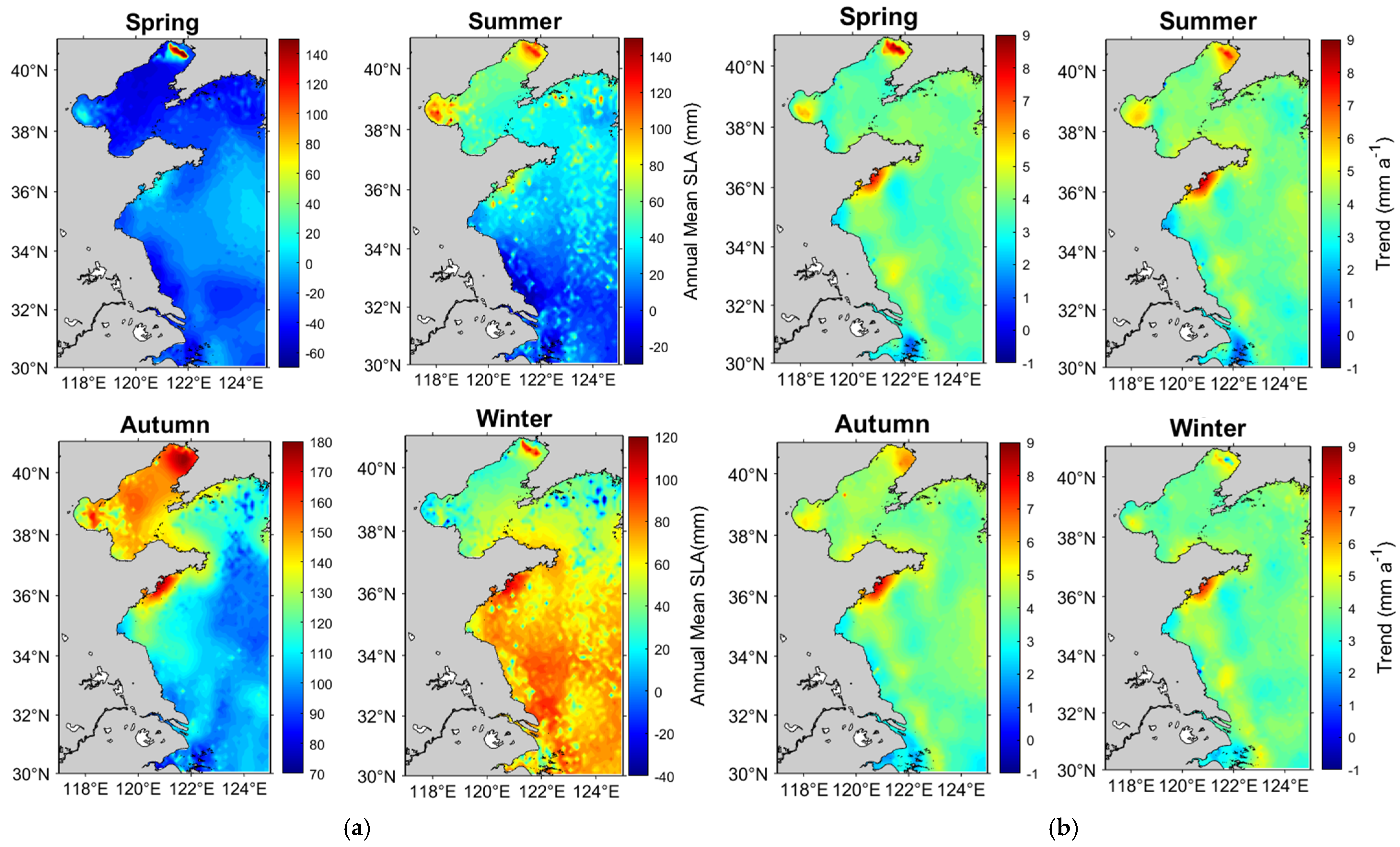
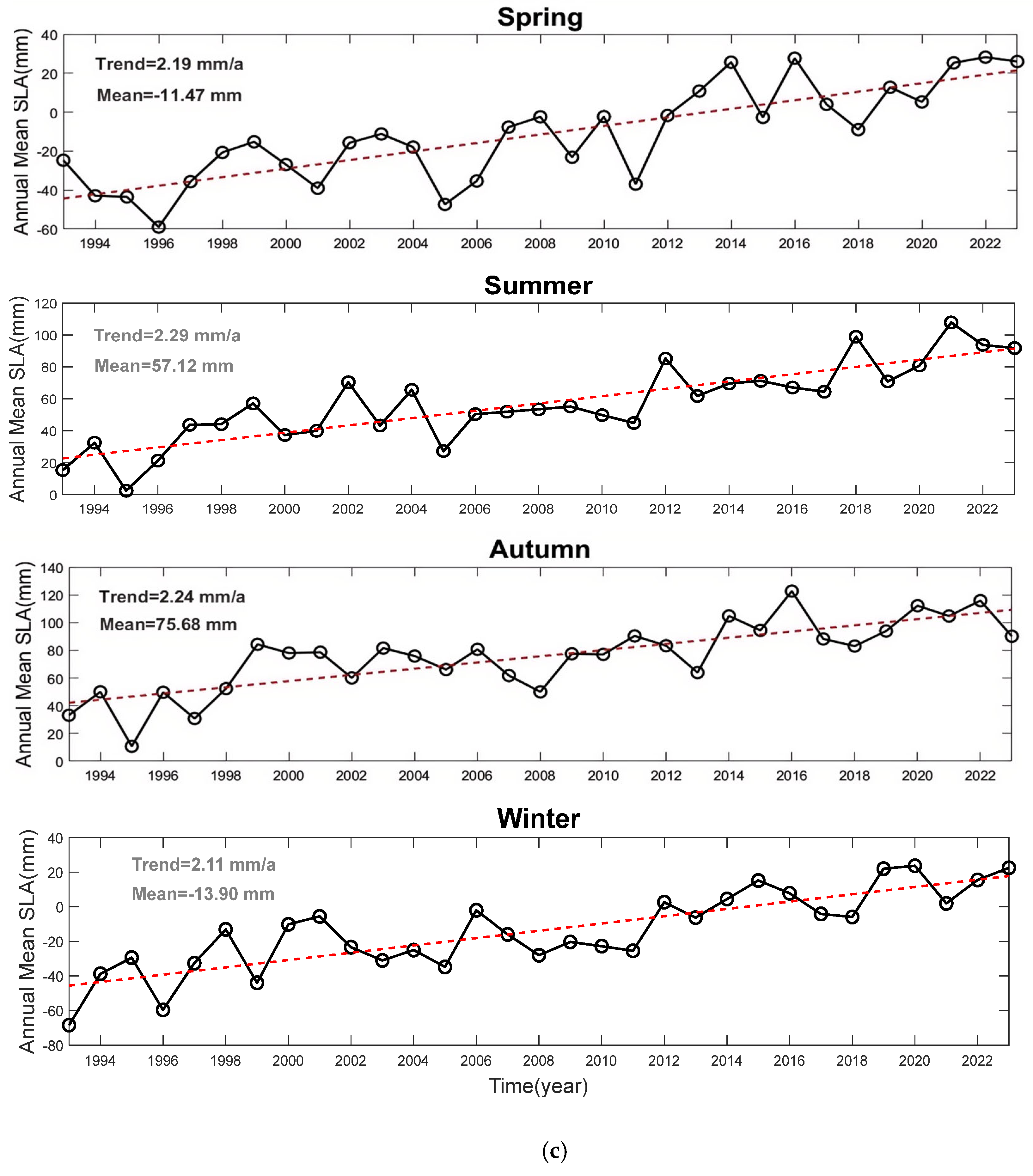
4.1. Spatiotemporal Variation of SLA in the Bohai Sea and Yellow Sea

In this study, an improved LMD method was applied to process the gridded satellite altimetry sea-level anomaly (SLA) data from January 1993 to December 2023. The LMD method decomposes the data into multi-scale components, with high-frequency components denoised using a moving average filter. After denoising, the data were reconstructed to obtain new time series that more accurately reflect the underlying trends while minimizing noise interference.

The spatial distribution of the multi-year average sea-level anomalies (SLA) for the YS and BS regions was calculated, revealing the long-term variations in sea-level trends (Figure 2). The analysis indicated that the sea-level anomalies in these regions exhibit both spatial and temporal variability, influenced by atmospheric pressure patterns, ocean currents, and regional climate fluctuations [22]. The northeastern marginal seas of the BS showed higher sea levels, while areas near Lianyungang in the YS also exhibited elevated sea levels. However, the rate of sea-level rise was higher near Lianyungang. Overall, the sea level in the YS and BS is rising, with regional variations in the rate of increase.

According to our results, the northern part of the Yellow Sea shows more significant SLA variability, especially near the Yangtze River estuary, where the amplitude of anomalies is notably pronounced (Figure 2b). On a decadal scale, these amplitude variations (Figure 2c) reflect large-scale interannual climate changes, influenced by global climate patterns such as the Pacific Decadal Oscillation (PDO), El Niño–Southern Oscillation (ENSO), and the Arctic Oscillation (AO) [23,24]. These long-term and short-term variations further illustrate the dynamic nature of sea-level anomalies in the region.

To analyze the temporal trends, the gridded data were averaged along latitude, and the multi-year average SLA time series was calculated. A linear trend was estimated for this time series to provide insights into the long-term evolution of sea levels in the study area (Figure 2d). The results indicated a positive trend in the sea-level anomaly over the study period, with a rate of change of 2.21 mm per year (mm/a). The multi-year average SLA value for the 31-year period is 26.86 mm. Notably, there was a sharp decline in sea level between 2004 and 2005, followed by a five-year continuous rise from 2017 to 2022. This observed trend aligns with previous studies that attributed long-term sea-level rise in the region to factors such as thermal expansion, glacial melting, and human-induced modifications to the hydrological cycle [25]. The abrupt decline in 2004–2005 is consistent with other regional studies that have documented short-term fluctuations in sea level, influenced by variations in atmospheric pressure, ocean currents, and climate events like El Niño and La Niña.

Annual variations in the YS and BS region are influenced by several environmental and climatic factors, including seasonal monsoon dynamics, freshwater input from rivers, and interannual variations in sea surface temperature. For instance, changes in the East Asian monsoon and large-scale oceanic circulation patterns have been shown to contribute to variations in sea level, particularly during warmer months when thermal expansion and freshwater influx are most pronounced. These processes, combined with regional atmospheric pressure systems, play a crucial role in shaping the seasonal and annual SLA patterns observed in the region [26].

4.2. EOF Analysis and Its Application to Oceanic Variations

We employed the EOF analysis method to decompose the annual sea-level variations in the YS and BS region, extracting the first three modes. The first mode accounted for 90.40% of the total variance, followed by the second (2.78%) and third (1.47%) modes (Figure 3). The first mode exhibits a basin-wide coherent variation pattern, reflecting the dominant influence of large-scale atmospheric forcing and seasonal thermal expansion on sea level. In the following sections, this primary mode will be further examined in relation to sea surface temperature (SST) and precipitation to explore its potential driving mechanisms.

The first EOF mode, which explains the majority of the variance, reflects large-scale sea-level changes driven by regional atmospheric and oceanic processes, particularly the East Asian monsoon and oceanic circulation patterns. The second mode highlights smaller, more localized variations, possibly related to seasonal changes, freshwater inputs from rivers, and regional climate fluctuations. The third mode, though contributing less to total variance, captures extreme climate events, human activities, and other anomalies. Despite its small contribution, the time coefficient amplitude is large, indicating strong short-term effects on sea-level variability during certain periods. These results suggest that sea-level anomalies are influenced by both natural factors (thermal expansion, ocean circulation) and anthropogenic factors (land reclamation, hydrological changes).

The findings align with previous studies, confirming that the region’s sea-level variations are shaped by a complex interplay of both natural and human-induced factors [27].

4.3. Correlation Analysis Between SST and SLA

The contribution of the first mode is the most significant. To further investigate its potential influences, we performed a correlation analysis between the first mode and the sea surface temperature (SST) data as well as precipitation grid data from the YS and BS region. This approach highlights the dominant role of the first mode in explaining variability in the region’s SST and precipitation patterns, which is critical for understanding the climatic processes in the YS and BS area.

The spatial distribution of sea surface temperature (SST) and its relationship with sea-level variability in the YS and BS are illustrated (Figure 4). The annual mean SST distribution is shown, which increases from south to north, with the YS having higher temperatures than the BS, reflecting the influence of latitude on temperature patterns (Figure 4a). A slight upward trend in SST is observed, particularly in the BS, indicating a stronger warming rate in this region (Figure 4b). This aligns with global trends suggesting that coastal and marginal seas are more responsive to warming due to localized climatic factors. The correlation between SST and SLA is presented, revealing a significant positive relationship, with most regions showing correlation coefficients exceeding 0.6 (Figure 4c). This indicates that SST, through mechanisms such as thermal expansion, plays a crucial role in driving sea-level rise. The stronger correlation observed in the YS, which is larger and deeper than the BS, further emphasizes the region’s heightened sensitivity to SST changes, influenced by more complex ocean circulation patterns and atmospheric conditions [28,29].

4.4. Correlation Analysis Between Precipitation and SLA

To further explore the impact of precipitation on sea level, we performed a correlation analysis between precipitation data and SLA (Figure 5).

The spatial distribution of annual average precipitation is shown, which exhibits a clear latitudinal gradient, with precipitation decreasing from south to north (Figure 5a). This trend is consistent with previous studies indicating a latitudinal decline in precipitation across East Asia [30]. The rate of change in annual precipitation is presented, revealing that the southern YS experiences a higher rate of increase compared to the northern regions (Figure 5b). The spatial correlation between precipitation and sea level is depicted, showing a positive correlation in the BS, where increased precipitation contributes to rising sea levels (Figure 5c). In contrast, a negative correlation is observed in the western YS, likely influenced by complex factors such as ocean dynamics and freshwater inputs. These correlations are statistically significant, as verified by significance tests. The BS, due to its shallowness, is highly sensitive to precipitation changes, with stronger correlations between precipitation and sea-level fluctuations. This is characteristic of shallow, semi-enclosed seas. In contrast, the western Yellow Sea’s negative correlation may result from factors like coastal upwelling, ocean circulation, and river discharge, which can offset the impact of precipitation. In conclusion, while precipitation affects sea-level changes in both seas, the relationship exhibits spatial variability. The shallowness of the Bohai Sea makes it particularly sensitive to precipitation, while the western sea areas exhibit more complex dynamics due to a combination of freshwater discharge, tidal mixing, and coastal currents from major rivers such as the Yellow and Yalu rivers. Additionally, the shallow topography of the region amplifies the effects of atmospheric forcing and seasonal hydrological variability, further influencing sea-level change.

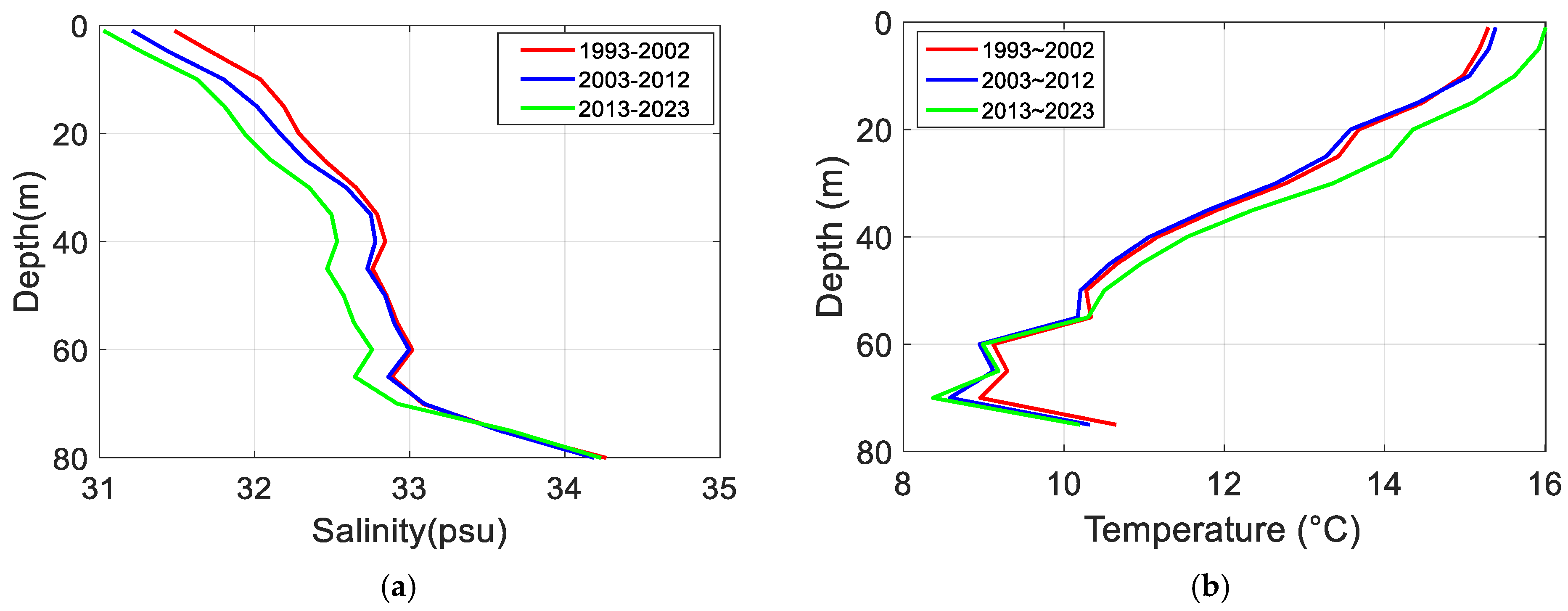
4.5. Temperature and Salinity Profiles and Their Impact on Sea-Level Changes

To further investigate the temperature and salinity characteristics of the YS and BS, we plotted the profiles of temperature and salinity variations with depth to reveal their depth-dependent changes (Figure 6).

The salinity profiles of the YS and BS regions over a decadal scale reveal a gradual decrease in salinity with increasing depth (Figure 6a). This trend is likely influenced by the increase in freshwater input from precipitation and river discharge, particularly during the warmer months, which leads to a stratified water column where fresher, lower-salinity water is concentrated at the surface, while more saline waters are deeper [31]. This change is also linked to the intensified seasonal monsoonal rainfall, which, along with the associated changes in sea surface temperature (SST), contributes to the reduction of salinity levels in coastal areas [32]. Moreover, changes in coastal currents and the influence of the Yangtze River discharge, which carries large amounts of freshwater into the YS, contribute to the observed decrease in salinity at shallower depths. In contrast, the temperature profiles of the YS and BS regions are presented, showing an increasing trend in temperature with depth over the same decadal period (Figure 6b). This warming trend with depth is likely due to the enhanced greenhouse effect, which has led to higher surface temperatures and a subsequent warming of the upper ocean layers. Additionally, oceanographic processes such as the weakening of upwelling and changes in the stratification of the water column may contribute to the observed temperature increase at deeper layers. According to Pei et al. [33], the deeper waters of the YS and BS are influenced by a combination of atmospheric warming and reduced vertical mixing, leading to temperature increases at depth. Moreover, long-term oceanographic shifts, including changes in circulation patterns and the warming of the East Asian seas due to global climate change, could also be key contributors to the observed trend [34,35]. In summary, salinity shows a decadal decrease with depth, influenced by freshwater inputs and seasonal hydrological changes (Figure 6a), while temperature increases with depth, likely driven by atmospheric warming and changes in oceanographic circulation patterns (Figure 6b).

In order to further explore the seasonal changes in the YS and BS region, our data analysis summarizes the influence of different seasons (spring: March to May, summer: June to August, autumn: September to November, winter: December to February) on sea-level fluctuations (Figure 7).

The seasonal spatiotemporal distribution and trend analysis of the sea-level anomaly (SLA) for the YS and BS region from January 1993 to December 2023 is presented (Figure 7). The spatial distribution of the annual mean SLA for each season (spring, summer, autumn, and winter) reveals distinct seasonal patterns, which are influenced by both atmospheric and oceanic processes. The spatiotemporal variation of sea-level anomaly (SLA) in the YS and BS regions was analyzed, along with corresponding changes in sea surface temperature (SST), precipitation, and salinity. The annual mean time series of these variables was calculated to examine their long-term trends and variability (

Table 1. Annual mean values and long-term trends of SLA, SST, precipitation, and salinity.

	Average Value (mm)					Average Annual Rate of Change
	Spr.	Sum.	Aut.	Win.		Spr.	Sum.	Aut.	Win.
SLA (mm)	−11.47	57.12	75.68	−13.90	SLA (mm/a)	2.190	2.291	2.236	2.113
SST (°C)	10.24	23.58	19.90	7.73	SST (°C/a)	0.028	0.020	0.022	0.009
Precipitation (mm)	2.10	5.29	2.03	1.04	Precipitation (mm/a)	−0.014	−0.023	0.011	−0.002
Salinity (psu)	31.69	19.05	31.17	31.82	Salinity (psu/a)	−0.010	−0.082	−0.011	−0.014

).

During the spring and summer months, higher sea-level anomalies are observed, particularly along the coastal regions, which can be attributed to thermal expansion and increased precipitation during warmer months, as reported by previous studies [36]. The summer monsoon, which brings more rainfall and freshwater influx into the BS, tends to elevate local sea levels through freshwater input and changes in ocean currents. Conversely, during the autumn and winter months, the SLA decreases, which is likely related to the cooling of the water, atmospheric pressure systems, and the dominance of stronger cold air outbreaks that reduce regional sea-level height [37]. Furthermore, the rate of change in the SLA over these seasons (Figure 7b) shows significant variability. The spring and summer months exhibit a higher rate of change, indicating more pronounced seasonal fluctuations in sea-level anomaly. In contrast, autumn and winter exhibit more moderate changes in sea level, reflecting the relative stability of the oceanic system during colder months.

The time series of SLA for each season (Figure 7c) indicates that the seasonal trends are largely consistent over the study period, with notable fluctuations in sea level during the summer months. The linear trend estimation suggests that, overall, the seasonal sea-level anomalies have slightly increased over the past three decades, with higher anomalies observed in summer compared to winter, indicating an intensification of seasonal variation in the region.

In order to gain deeper insights into the decadal-scale amplitude variations, we performed calculations of the amplitudes for SLA, SST, precipitation, and salinity (

Table 2. Decadal-scale amplitudes of SLA, SST, precipitation, and salinity.

	SLA (mm)	SST (°C)	Precipitation (mm)	Salinity (psu)
Spring	3.951	0.152	0.108	0.087
Summer	5.098	0.145	0.418	0.860
Autumn	5.155	0.179	0.112	0.113
Winter	0.193	0.124	0.105	0.095

).

The impacts of precipitation and salinity on sea-level variations are more pronounced during the summer, primarily reflected in the changes of steric sea level (Table 2). In contrast, SST variations on the decadal scale are relatively minor. Sea-level anomalies (SLA) exhibit a clear seasonal variation pattern, with more significant changes occurring in summer and autumn [38]. Overall, at the decadal seasonal scale, variations in SST, precipitation, and salinity collectively influenced sea-level changes [39]. The correlations between SST, precipitation, and the first mode of SLA at the annual scale were analyzed, revealing distinct spatial distribution patterns (Figure 4 and Figure 5). Our study highlights several potential factors driving sea-level variability and provides valuable insights for future research.

5. Conclusions

This study systematically analyzed sea-level changes in the YS and BS from 1993 to 2023 based on satellite altimetry data. Using local model decomposition (LMD) to reconstruct gridded sea-level data, the study found an average sea-level rise of 28.86 mm/a, with an average increase rate of 2.21 mm/a. Empirical Orthogonal Function (EOF) analysis revealed that the first mode explained most of the variance, reflecting large-scale sea-level changes driven by regional atmospheric and oceanic processes, particularly the East Asian monsoon, ocean circulation patterns, temperature variations, and precipitation, all of which contribute to sea-level rise. The second mode captured smaller, more localized variations, likely linked to seasonal changes, riverine freshwater inputs, and regional climate fluctuations. The third mode, although contributing less, captured the influence of extreme climatic events and human activities on sea-level changes.

Correlation analysis indicated a significant relationship between the first mode and sea surface temperature (SST) and precipitation, further confirming that sea-level variability in the region is influenced by both natural drivers and anthropogenic factors. The study also found that the shallow BS is more sensitive to precipitation changes, while the YS is influenced by more complex factors such as ocean circulation and upwelling. Additionally, seasonal sea-level anomalies (SLA) exhibited clear seasonal patterns, with higher anomalies observed in summer and autumn, mainly due to thermal expansion and increased precipitation.

On a decadal scale, temperature and salinity profiles revealed a trend of increasing temperatures and decreasing salinity with depth, likely driven by freshwater inputs and seasonal hydrological changes. The decadal warming trend, particularly in deeper layers, reflects the ongoing impact of climate change. The study also highlighted that the YS, with its more complex ocean circulation, is more sensitive to SST variations compared to the BS.

Overall, this study provides new insights into the dynamics of sea-level fluctuations, emphasizing both natural and human-induced drivers. It contributes to a better understanding of the joint effects of climate change, human activities, and oceanic processes on sea-level variability, offering a valuable foundation for future research.

References

1. Liu, Y.; Wang, Z.; Yang, X.; Wang, S.; Liu, X.; Liu, B.; Zhang, J.; Meng, D.; Ding, K.; Gao, K.; et al. Changes in the spatial distribution of mariculture in China over the past 20 years. J. Geogr. Sci. 2023, 33, 2377–2399. [Google Scholar] [CrossRef]
2. Song, J.; Duan, L. The Bohai sea. In World Seas: An Environmental Evaluation; Academic Press: Cambridge, MA, USA, 2019; pp. 377–394. [Google Scholar]
3. Zhang, Z.; Yang, W.; Ding, J.; Sun, T.; Liu, H.; Liu, C. Identifying changes in China’s Bohai and Yellow Sea fisheries resources using a causality-based indicator framework, convergent cross-mapping, and structural equation modeling. Environ. Sustain. Indic. 2022, 14, 100171. [Google Scholar] [CrossRef]
4. Cheng, Y.; Plag, H.; Hamlington, B.; Xu, Q.; He, Y. Regional sea level variability in the Bohai sea, Yellow sea, and East china sea. Cont. Shelf Res. 2015, 111, 95–107. [Google Scholar] [CrossRef]
5. Li, Y.; Zhang, H.; Tang, C.; Zou, T.; Jiang, D. Influence of rising sea level on tidal dynamics in the Bohai Sea. J. Coast. Res. 2016, 74, 22–31. [Google Scholar] [CrossRef]
6. Feng, X.; Feng, H.; Li, H.; Zhang, F.; Feng, W.; Zhang, W.; Yuan, J. Tidal responses to future sea level trends on the Yellow Sea shelf. J. Geophys. Res. Ocean. 2019, 124, 7285–7306. [Google Scholar] [CrossRef]
7. Jian, M.; Fangli, Q.; Changshui, X.; Yongzeng, Y. Tidal effects on temperature front in the Yellow Sea. Chin. J. Oceanol. Limnol. 2004, 22, 314–321. [Google Scholar] [CrossRef]
8. Lu, J.; Qiao, F.; Wang, X.; Wang, Y.; Teng, Y.; Xia, C. A numerical study of transport dynamics and seasonal variability of the Yellow River sediment in the Bohai and Yellow seas. Estuar. Coast. Shelf Sci. 2011, 95, 39–51. [Google Scholar] [CrossRef]
9. Cheng, Y.; Ezer, T.; Atkinson, L.P.; Xu, Q. Analysis of tidal amplitude changes using the EMD method. Cont. Shelf Res. 2017, 148, 44–52. [Google Scholar] [CrossRef]
10. Jin, T.; Xiao, M.; Jiang, W.; Shum, C.K.; Ding, H.; Kuo, C.; Wan, J. An adaptive method for nonlinear sea level trend estimation by combining EMD and SSA. Earth Space Sci. 2021, 8, e2020EA001300. [Google Scholar] [CrossRef]
11. Chen, H.; Lu, T.; Huang, J.; He, X.; Sun, X. An improved VMD–EEMD–LSTM time series hybrid prediction model for sea surface height derived from satellite altimetry data. J. Mar. Sci. Eng. 2023, 11, 2386. [Google Scholar] [CrossRef]
12. Kenigson, J.; Han, W. Detecting and understanding the accelerated sea level rise along the east coast of the United States during recent decades. J. Geophys. Res. Ocean. 2014, 119, 8749–8766. [Google Scholar] [CrossRef]
13. Chen, X.; Zhao, X.; Liang, Y.; Luan, X. Ocean turbulence denoising and analysis using a novel EMD-based denoising method. J. Mar. Sci. Eng. 2022, 10, 663. [Google Scholar] [CrossRef]
14. Wei, Z.; Ren, C.; Liang, X.; Liang, Y.; Yin, A.; Liang, J.; Yue, W. Sea-Level Estimation from GNSS-IR under Loose Constraints Based on Local Mean Decomposition. Sensors 2023, 23, 6540. [Google Scholar] [CrossRef] [PubMed]
15. Smith, J. The local mean decomposition and its application to EEG perception data. J. R. Soc. Interface 2005, 2, 443–454. [Google Scholar] [CrossRef]
16. Lorenz, E.N. Empirical Orthogonal Functions and Principal Component Analysis. J. Atmos. Sci. 1956, 13, 603–607. [Google Scholar]
17. Kutzbach, J.E. Empirical Eigenvectors of Sea-Level Pressure, with Application to Long-Period Fluctuations in the Southern Oscillation. Mon. Weather Rev. 1967, 95, 1–11. [Google Scholar]
18. Niedzielski, T.; Kosek, W. Forecasting sea level anomalies from TOPEX/Poseidon and Jason-1 satellite altimetry. J. Geod. 2009, 83, 469–476. [Google Scholar] [CrossRef]
19. Li, W.; Wang, H.; Xiang, W.; Wang, A.-M.; Xu, W.-Q.; Jiang, Y.-X.; Wu, X.-H.; Quan, M.-Y. Sea-level change in coastal areas of China: Status in 2021. Adv. Clim. Change Res. 2024, 15, 515–524. [Google Scholar] [CrossRef]
20. Cazenave, A.; Dominh, K.; Gennero, M.; Ferret, B. Global mean sea level changes observed by Topex-Poseidon and ERS-1. Phys. Chem. Earth 1998, 23, 1069–1075. [Google Scholar] [CrossRef]
21. Geng, X. Decadal and Subseasonal Variations of ENSO Impacts on the East Asian Winter Climate and Their Mechanisms. Ph.D. Thesis, Nanjing University of Information Science and Technology, Nanjing, China, 2018. [Google Scholar]
22. Liu, H.; Cheng, X.; Qin, J.; Zhou, G.; Jiang, L. The dynamic mechanism of sea level variations in the Bohai Sea and Yellow Sea. Clim. Dyn. 2023, 61, 2937–2947. [Google Scholar] [CrossRef]
23. Wei, H.; Zhang, H.; Yang, W.; Feng, J.; Zhang, C. The changing Bohai and Yellow Seas: A physical view. Chang. Asia-Pac. Marg. Seas 2020, 105–120. Available online: https://link.springer.com/chapter/10.1007/978-981-15-4886-4_7 (accessed on 15 December 2024).
24. Han, G.; Huang, W. Pacific decadal oscillation and sea level variability in the Bohai, Yellow, and East China Seas. J. Phys. Oceanogr. 2008, 38, 2772–2783. [Google Scholar] [CrossRef]
25. Cheng, Y.; Ezer, T.; Hamlington, B. Sea level acceleration in the China Seas. Water 2016, 8, 293. [Google Scholar] [CrossRef]
26. Marcos, M.; Tsimplis, M.; Calafat, F. Inter-annual and decadal sea level variations in the north-western Pacific marginal seas. Prog. Oceanogr. 2012, 105, 4–21. [Google Scholar] [CrossRef]
27. Guo, J.; Hu, Z.; Wang, J.; Chang, X.; Li, G. Sea level changes of China seas and neighboring ocean based on satellite altimetry missions from 1993 to 2012. J. Coast. Res. 2015, 73, 17–21. [Google Scholar] [CrossRef]
28. Lima, F.P.; Wethey, D.S. Three decades of high-resolution coastal sea surface temperatures reveal more than warming. Nat. Commun. 2012, 3, 704. [Google Scholar] [CrossRef]
29. Feng, C.; Yin, W.; He, S.; He, M.; Li, X. Evaluation of SST data products from multi-source satellite infrared sensors in the Bohai-Yellow-East China Sea. Remote Sens. 2023, 15, 2493. [Google Scholar] [CrossRef]
30. Lai, Y.; Dzombak, D. Use of Historical Data to Assess Regional Climate Change. J. Clim. 2019, 32, 4299–4320. [Google Scholar] [CrossRef]
31. Yanagi, T.; Takahashi, S. Seasonal variation of circulations in the East China Sea and the Yellow Sea. J. Oceanogr. 1993, 49, 503–520. [Google Scholar] [CrossRef]
32. Zhang, Z.; Qiao, F.; Guo, J.; Guo, B. Seasonal changes and driving forces of inflow and outflow through the Bohai Strait. Cont. Shelf Res. 2018, 154, 1–8. [Google Scholar] [CrossRef]
33. Pei, Y.; Liu, X.; He, H. Interpreting the sea surface temperature warming trend in the Yellow Sea and East China Sea. Sci. China Earth Sci. 2017, 60, 1558–1568. [Google Scholar] [CrossRef]
34. Ma, S.; Liu, Y.; Li, J.; Fu, C.; Ye, Z.; Sun, P.; Yu, H.; Cheng, J.; Tian, Y. Climate-induced long-term variations in ecosystem structure and atmosphere-ocean-ecosystem processes in the Yellow Sea and East China Sea. Prog. Oceanogr. 2019, 175, 183–197. [Google Scholar] [CrossRef]
35. Liu, H.; Pang, C.; Yang, D.; Liu, Z. Seasonal variation in material exchange through the Bohai Strait. Cont. Shelf Res. 2021, 231, 104599. [Google Scholar] [CrossRef]
36. Bao, X.; Li, N.; Wu, D. Observed characteristics of the North Yellow Sea water masses in summer. Chin. J. Oceanol. Limnol. 2010, 28, 160–170. [Google Scholar] [CrossRef]
37. Zhao, G.; Jiang, W.; Wang, T.; Chen, S.; Bian, C. Decadal variation and regulation mechanisms of the suspended sediment concentration in the Bohai Sea, China. J. Geophys. Res. Ocean. 2022, 127, e2021JC017699. [Google Scholar] [CrossRef]
38. Ji, F.; Xiong, X.; Yang, J.; Liu, Y.; Han, L.; Dong, M.; Xu, S. Local freshwater fluxes determine salinity variations of the Bohai Sea: Based on 60 years of observations. Reg. Stud. Mar. Sci. 2024, 80, 103899. [Google Scholar] [CrossRef]
39. Lin, C.; Su, J.; Xu, B.; Tang, Q. Long-term variations of temperature and salinity of the Bohai Sea and their influence on its ecosystem. Prog. Oceanogr. 2001, 49, 7–19. [Google Scholar] [CrossRef]
Figure 1. Study area map of the Bohai Sea and Yellow Sea.
Jmse 13 01081 g001
Figure 2. Spatiotemporal distribution and trend analysis of satellite altimetry sea-level anomaly (SLA) from January 1993 to December 2023. (a) Multi-year average SLA spatial distribution. (b) Rate of change of multi-year average SLA spatial distribution. (c) Interannual SLA amplitude spatial distribution over a ten-year period. (d) Annual mean SLA time series with linear trend.
Jmse 13 01081 g002
Figure 3. The first three EOF modes of the Yellow and Bohai Sea region based on annual variations.
Jmse 13 01081 g003aJmse 13 01081 g003b
Figure 4. Spatial patterns of annual mean SST, its trend, and its relationship with the first EOF mode in the Yellow and Bohai Sea region. (a) Spatial distribution of the annual mean Sea Surface Temperature (SST). (b) Spatial distribution of the annual mean SST trend. (c) Spatial distribution of the correlation coefficients between the first mode of EOF analysis and SST.
Jmse 13 01081 g004
Figure 5. Spatial patterns of annual mean precipitation, its trend, and its relationship with the first EOF mode in the Yellow and Bohai Sea region. (a) Spatial distribution of the annual mean precipitation. (b) Spatial distribution of the annual mean precipitation trend. (c) Spatial distribution of the correlation coefficients between the first EOF mode and precipitation.
Jmse 13 01081 g005
Figure 6. Profiles of temperature and salinity in the Bohai and Yellow Seas from 1993 to 2020 as a function of depth. (a) Salinity profiles with depth on a decadal scale. (b) Temperature profiles with depth on a decadal scale.
Jmse 13 01081 g006
Figure 7. Seasonal spatiotemporal distribution and trend analysis of satellite altimetry sea-level anomaly (SLA) from January 1993 to December 2023. (a) Spatial distribution of the annual mean SLA for each season (spring, summer, autumn, winter) from January 1993 to December 2023 based on satellite altimetry. (b) Spatial distribution of the rate of change of annual mean SLA for each season (spring, summer, autumn, winter) from January 1993 to December 2023. (c) Time series of annual mean SLA for each season (spring, summer, autumn, winter) from January 1993 to December 2023 with linear trend estimation.
Jmse 13 01081 g007aJmse 13 01081 g007b