A Spatio-Temporal Graph Neural Network for Predicting Flow Fields on Unstructured Grids with the SUBOFF Benchmark

Abstract

To overcome the limitations of traditional convolutional and recurrent neural networks in capturing spatio-temporal dynamics in flow fields on unstructured grids, this study proposes a novel Spatio-Temporal Graph Neural Network (ST-GNN) model that integrates a Graph Neural Network (GNN) with a Long Short-Term Memory (LSTM) network. The GNN component captures spatial dependencies among irregular grid nodes via message passing, while the LSTM component models temporal evolution through gated memory mechanisms. This hybrid framework enables the joint learning of spatial and temporal features in complex flow systems. Two variants of ST-GNN, namely, GCN-LSTM and GAT-LSTM, were developed and evaluated using the SUBOFF AFF-8 benchmark dataset. The results show that GAT-LSTM achieved higher accuracy than GCN-LSTM, with average relative errors of 2.51% for velocity and 1.43% for pressure at the 1000th time step. Both models achieved substantial speedups over traditional CFD solvers, with GCN-LSTM and GAT-LSTM accelerating predictions by approximately 350 and 150 times, respectively. These findings position ST-GNN as an efficient and accurate alternative for spatio-temporal flow modeling on unstructured grids, advancing data-driven fluid dynamics.

1. Introduction

The spatio-temporal evolution of complex vortex flow fields surrounding underwater vehicles plays a critical role in determining their maneuverability, stealth performance, and operational safety. Therefore, accurately characterizing and predicting these vortex dynamics is essential to achieving optimal hydrodynamic design and overall engineering performance. Traditionally, investigations into such flow fields have relied on towing tank experiments and numerical simulations using computational fluid dynamics (CFD). However, physical experiments are often constrained by high costs, extended testing durations, and limitations in replicating extreme operational conditions. On the other hand, high-fidelity CFD simulations require tens to hundreds of millions of computational grid elements to capture large-scale, highly complex flow phenomena, thereby imposing substantial computational burdens.

In recent years, the rapid advancement of artificial intelligence has introduced a transformative paradigm in addressing computational fluid dynamics (CFD) challenges, leading to the emergence of the interdisciplinary field of Artificial Intelligence for Computational Fluid Dynamics (AI for CFD) [1,2,3]. Among various approaches, Deep Neural Network (DNN)-based models have become a central research focus in flow field prediction, with substantial progress achieved using Recurrent Neural Networks (RNNs), Convolutional Neural Networks (CNNs), and Physics-Informed Neural Networks (PINNs). RNN-based models exhibit strong capabilities in capturing the temporal evolution of flow fields and have been successfully applied to turbulence prediction tasks [4,5,6]. CNNs, through hierarchical convolution and pooling operations, are effective at extracting spatial features and have shown promising results for reconstructing vortex structures [7,8,9]. To more precisely capture the spatio-temporal features of flow field data, several researchers have investigated hybrid neural network architectures integrating RNNs and CNNs for enhanced prediction. These studies have verified that RNN-CNN hybrid models can achieve high prediction accuracy and strong generalization performance when modeling the spatio-temporal evolution of complex, unsteady flow fields [10,11]. PINNs incorporate physical governing equations directly into the loss function, enabling the training process to adhere to physical laws and thereby improving model generalization, particularly under conditions of sparse flow field data [12,13,14] Nevertheless, existing DNN architectures, including RNNs, CNNs, and PINNs, are fundamentally designed for data defined on regular Euclidean grids and therefore struggle to capture the complex spatial topologies of unstructured grid flow field data. Such unstructured representations are prevalent in large-scale, highly intricate systems, including underwater vehicles and submarines.

A Graph Neural Network (GNN) is a deep learning model designed for graph-structured data (nodes, edges) that effectively handles non-Euclidean data structures, thereby offering a novel approach for modeling and predicting unstructured flow fields. Current researchers have applied GNN-based methods to predict flow fields around unstructured grid geometries, such as cylinders and airfoils. Pfaff et al. (2020) proposed a Mesh-Based Simulation with Graph Networks (MeshGraphNet) model to predict the flow fields of cylinders and NACA airfoils, as well as structural dynamic responses and the behavior of deformable materials, establishing an important foundation for applying GNNs to fluid and structural field prediction [15]. Subsequently, many scholars focused on improving and optimizing methods based on the MeshGraphNet. Fortunato et al. (2022) introduced a multilevel approach that enhanced prediction accuracy and reduced computational costs compared to the original MeshGraphNet [16]. Yang et al. (2022) proposed Algebraic Multigrid Net (AMGNet), which integrates algebraic multigrid techniques into the MeshGraphNet architecture, and successfully applied it to predict flow fields around cylinders and airfoils [17]. Li et al. (2024) introduced the Finite Volume Graph Network (FVGN) and its improved model (Gen-FVGN), which enable prediction of cylinder and airfoil flow fields simulated using the finite volume method while retaining the “encoder–processor–decoder” core architecture of MeshGraphNet [18,19]. In the same year, a Finite Difference Informed Graph Network (FDGN) was introduced, which integrates graph networks with finite-difference techniques to predict flow fields with reduced dependence on labeled data while still preserving the core MeshGraphNet architecture [20].

Concurrently, significant research efforts have been directed towards applying fundamental GNN architectures like Graph Convolutional Networks (GCNs) and Graph Attention Networks (GAT) to fluid flow problems. These studies have demonstrated the versatility and effectiveness of GNNs in handling the unstructured data inherent to complex flow simulations. For instance, Ogoke et al. (2021) utilized a GCNN to predict global properties like drag force from scattered, irregular velocity measurements around airfoils, showcasing the model’s invariance to node order and resolution [21]. Peng et al. (2022) developed a GCN-based reduced-order model demonstrating excellent adaptability to non-uniform meshes and achieving a three-order-of-magnitude speedup while maintaining high accuracy for internal flow cases [22]. Furthermore, Liu et al. (2022) proposed a Graph Attention network-based Fluid simulation Model that leverages attention mechanisms to handle non-equilibrium phenomena in vortices and turbulent flows, reporting a speedup of two to three orders of magnitude over traditional CFD solvers for 2D cylinder flow [23]. Beyond these foundational works on canonical geometries, recent advancements have expanded the application of GNN to more complex and diverse scenarios. Covoni et al. (2024) demonstrated the capability of GNNs to predict explosion-induced transient flow in highly complex geometries, with strong generalization to domains significantly larger than those in the training set [24]. Hadizadeh et al. (2024) employed a GNN as a surrogate for multi-objective fluid-acoustic shape optimization, achieving high predictive accuracy for varied airfoil shapes and enabling drastic computational acceleration [25]. Gao et al. (2025) presented a reduced-dimensional deep learning approach leveraging GNN principles for fast 3D indoor flow field prediction with near-real-time inference [26]. Chen et al. (2025) introduced a Physics-Informed GNN for flow in porous media, rigorously enforcing physical constraints and outperforming traditional PINN [27]. A comprehensive review by Cheng et al. (2025) further synthesized these progresses, highlighting the pivotal role of GNN and other advanced ML methods in tackling unstructured grid data across computational physics [28].

While single GNN-based models effectively extract spatial features from unstructured grid flow field data, they struggle with long-term temporal prediction because they neglect the temporal evolution inherent in unsteady flow fields. To address this limitation, we propose a Spatio-temporal Graph Neural Network (ST-GNN) model that integrates a Graph Neural Network (GNN) with a Long Short-Term Memory (LSTM) network. This model leverages the GNN’s message-passing mechanism to capture spatial relationships among unstructured grid nodes and employs the LSTM’s gated memory mechanism to learn temporal evolution patterns of physical quantities, thereby enabling simultaneous modeling of spatial and temporal features in complex flow fields. We evaluate the accuracy and efficiency of two variants, namely, GCN-LSTM and GAT-LSTM, for predicting the spatio-temporal evolution of the DARPA SUBOFF AFF-8 flow field, which is characterized by complex unstructured grids.

It is important to clarify the research scope and comparison design of this study. The core objective is to evaluate the feasibility and effectiveness of the ST-GNN architecture for predicting the spatio-temporal evolution of complex unstructured grid flow fields surrounding underwater vehicles, with the SUBOFF AFF-8 serving as a representative benchmark. Within this scope, we focus on two variants of the framework: GCN-LSTM and GAT-LSTM. This choice is motivated by the fact that the GCN and GAT are currently the most widely used and representative GNN architectures, and their integration with temporal modeling mechanisms (LSTM) is directly relevant to assessing the applicability of the ST-GNN framework in complex flow scenarios. By comparing these two variants, we aim to demonstrate how different spatial feature extraction mechanisms affect the accuracy of spatio-temporal modeling for complex underwater vehicle flow fields, an issue that remains insufficiently addressed in existing studies that primarily focus on simple geometries.

The key contributions of this paper are as follows:

• A novel ST-GNN framework integrating a GNN and LSTM was proposed to jointly capture spatial dependencies and temporal dynamics in unstructured grid flow fields, addressing the limitation of traditional DNNs in handling non-Euclidean data.
• Two ST-GNN variants (GCN-LSTM and GAT-LSTM) were developed and compared; on the SUBOFF AFF-8 benchmark, both showed superior accuracy and computational efficiency over conventional CFD methods.
• The temporal generalization of the proposed models was evaluated, verifying their potential for accurate long-term prediction in complex unsteady flow scenarios.

The rest of the paper is organized as follows. Section 2 outlines the fluid dynamics governing equations used in the numerical simulation of the SUBOFF AFF-8 flow field. Section 3 details the proposed ST-GNN model and its underlying principles. Section 4 presents the CFD modeling and simulation calibration results for SUBOFF AFF-8, including a case study comparing flow field predictions from GAT-LSTM and GCN-LSTM. Section 5 assesses the temporal generalization capability of GAT-LSTM and GCN-LSTM. Finally, Section 6 summarizes this study with key findings and conclusions.

2. Governing Equations

The Reynolds-Averaged Navier–Stokes (RANS) method was employed to simulate the flow field around the SUBOFF AFF-8 model in this study. The governing equations of incompressible viscous fluids include the continuity equation and RANS equations, which can be expressed in the following form:

$${\displaystyle \frac{\partial {\overline{u}}_i}{\partial x_i}}=0\left(i=1,2,3\right)$$

(1)

$${\displaystyle \frac{\partial {\overline{u}}_i}{\partial t}}+{\overline{u}}_j{\displaystyle \frac{\partial {\overline{u}}_i}{\partial x_j}}={\overline{F}}_i-{\displaystyle \frac{1}{\rho }}{\displaystyle \frac{\partial \overline{p}}{\partial x_i}}+\nu {\displaystyle \frac{{\partial }^2{\overline{u}}_i}{\partial x_j\partial x_j}}-{\displaystyle \frac{\partial {\tau }_{ij}}{\partial x_j}}$$

(2)

where ρ is the fluid density, ${\overline{u}}_i$ is the time-averaged velocity component, $x_i$ is the Cartesian coordinate component, $\overline{p}$ is the time-averaged pressure, $\nu$ is the kinematic viscosity, and ${\tau }_{\mathrm{ij}}=\overline{{\mathrm{u}}_{\mathrm{i}}^{\prime }{\mathrm{u}}_{\mathrm{j}}^{\prime }}$ is the Reynolds stress tensor.

In this paper, the shear stress transport (SST) k-ω turbulence model was utilized to provide closure for these equations, and the governing equations are as follows:

Transport equation for turbulent kinetic energy (k):

$${\displaystyle \frac{\partial \left(\rho k\right)}{\partial t}}+{\displaystyle \frac{\partial \left(\rho u_{j}k\right)}{\partial x_j}}=P_k-{\beta }^{*}\rho \omega k+{\displaystyle \frac{\partial }{\partial x_j}}\left[\left(\mu +{\sigma }_k{\mu }_t\right){\displaystyle \frac{\partial k}{\partial x_j}}\right]$$

(3)

Transport equation for the specific dissipation rate (ω):

$${\displaystyle \frac{\partial \left(\rho \omega \right)}{\partial t}}+{\displaystyle \frac{\partial \left(\rho u_j\omega \right)}{\partial x_j}}=\alpha {\displaystyle \frac{\omega }{k}}{P}_k-\beta \rho {\omega }^2+{\displaystyle \frac{\partial }{\partial x_j}}\left[\left(\mu +{\sigma }_{\omega }{\mu }_t\right){\displaystyle \frac{\partial \omega }{\partial x_j}}\right]+2\left(1-F_1\right)\rho {\sigma }_{\omega 2}{\displaystyle \frac{1}{\omega }}{\displaystyle \frac{\partial k}{\partial x_j}}{\displaystyle \frac{\partial \omega }{\partial x_j}}$$

(4)

where $P_k$ is the production term for turbulent kinetic energy, ${\mu }_{\mathrm{t}}$ is the turbulent viscosity, and $F_1$ is the blending function.

The mathematical expression for the blending function and related terms is as follows:

$$P_k=min\left({\mu }_t{\displaystyle \frac{\partial u_i}{\partial x_j}}\left({\displaystyle \frac{\partial u_i}{\partial x_j}}+{\displaystyle \frac{\partial u_j}{\partial x_i}}\right),10{\beta }^{*}\rho \omega k\right)$$

(5)

$${\mu }_t={\displaystyle \frac{\rho a_{1}k}{max\left(a_1\omega ,S{F}_2\right)}}$$

(6)

$$F_1=tanh\left(ar{g}_1^4\right), ar{g}_1=min\left[max\left({\displaystyle \frac{\sqrt{k}}{{\beta }^{*}\omega y}},{\displaystyle \frac{500\nu }{y^2\omega }}\right),{\displaystyle \frac{4\rho {\sigma }_{\omega 2}k}{C{D}_{k\omega }{y}^2}}\right]$$

(7)

where S is the magnitude of the strain rate tensor, $F_2$ is the function for shear stress correction, y is the distance to the nearest wall, β* is a model constant, and $C{D}_{k\omega }$ is the coefficient for the cross-diffusion term, expressed as:

$$S=\sqrt{2S_{ij}{S}_{ij}},S_{ij}={\displaystyle \frac{1}{2}}\left({\displaystyle \frac{\partial u_i}{\partial x_j}}+{\displaystyle \frac{\partial u_j}{\partial x_i}}\right)$$

(8)

$$F_2=tanh\left(ar{g}_2^2\right),ar{g}_2=max\left({\displaystyle \frac{2\sqrt{k}}{{\beta }^{*}\omega y}},{\displaystyle \frac{500\nu }{y^2\omega }}\right)$$

(9)

$$C{D}_{k\omega }=max\left(2\rho {\sigma }_{\omega 2}{\displaystyle \frac{1}{\omega }}{\displaystyle \frac{\partial k}{\partial x_j}}{\displaystyle \frac{\partial \omega }{\partial x_j}},{10}^{-10}\right)$$

(10)

The constants, such as turbulent kinetic energy diffusion coefficients ${\sigma }_k$, specific dissipation rate diffusion coefficients ${\sigma }_{\omega }$, generation term coefficients $\alpha$, and dissipation term coefficients $\beta$, were calculated using the following equations:

$$\phi =F_1{\phi }_1+\left(1-F_1\right){\phi }_2,\left(\phi ={\sigma }_k,{\sigma }_{\omega },\beta ,\alpha \right)$$

(11)

$${\alpha }_1={\displaystyle \frac{{\beta }_1}{{\beta }^{*}}}-{\displaystyle \frac{{\sigma }_{\omega 1}{\kappa }^2}{\sqrt{{\beta }^{*}}}},{\alpha }_2={\displaystyle \frac{{\beta }_2}{{\beta }^{*}}}-{\displaystyle \frac{{\sigma }_{\omega 2}{\kappa }^2}{\sqrt{{\beta }^{*}}}}$$

(12)

where ${\phi }_1$ and ${\phi }_2$ represent sets of constants for the inner and outer layers in the blending function.

3. Methodology

This section presents the ST-GNN framework. It covers the overall structure, GNN-based encoder, and LSTM-based decoder. The goal is to clarify how ST-GNN captures spatio-temporal features of flow fields on unstructured grids.

3.1. Framework of ST-GNN

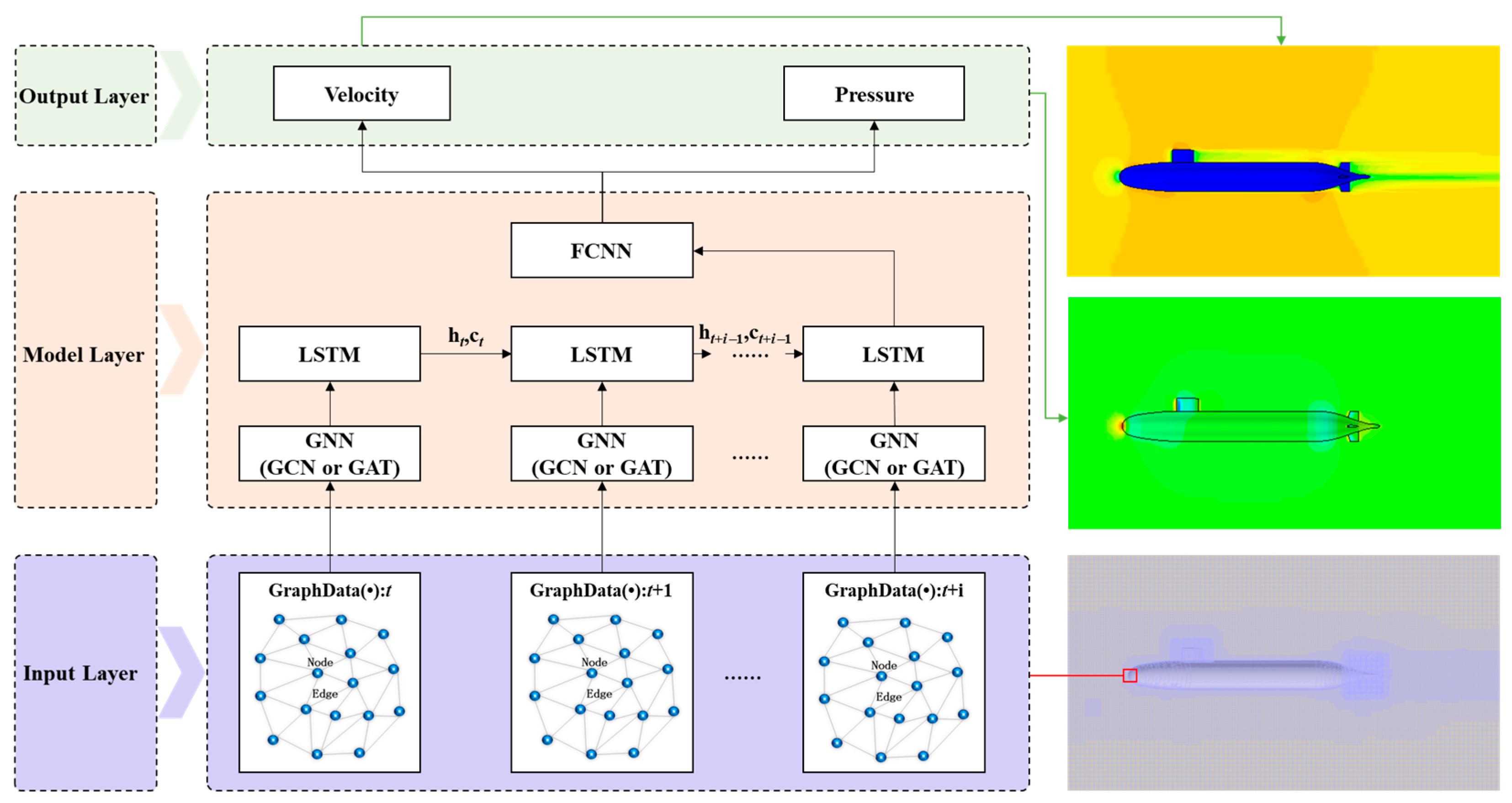
The ST-GNN framework proposed in this study comprises a Graph Neural Network (GNN) encoder coupled with an LSTM-based decoder, as illustrated in Figure 1. Two architectural variants were implemented: GCN-LSTM, which employs a Graph Convolutional Network encoder, and GAT-LSTM, which incorporates a Graph Attention Network encoder. Both variants share an identical LSTM decoding structure.

Training data were obtained from the SUBOFF AFF-8 unstructured grid dataset, consisting of time-sequential three-dimensional velocity and pressure fields formatted as graph-structured inputs. The GNN encoder extracted spatial dependencies among grid nodes through a message-passing mechanism, via neighborhood aggregation in the GCN or attention weighting in GAT, and mapped the inputs into a high-dimensional latent space. These latent spatial features were then processed by the LSTM decoder to capture the temporal evolution of the flow field.

Finally, a fully connected neural network (FCNN) transformed the decoded hidden features back into physical quantities, including velocity and pressure fields. By integrating spatial topology modeling with temporal sequence learning, the ST-GNN framework jointly captured the spatial structure and temporal evolution of the flow field, enabling accurate and computationally efficient predictions across complex unstructured domains.

3.2. Architecture of the GNN-Based Encoder

3.2.1. GCN Encoder

A GCN extends convolutional operations to non-Euclidean domains, enabling effective extraction of spatial patterns from irregular structures, such as unstructured grids. In our ST-GNN framework, the GCN encoder maps graph-structured flow field data from the SUBOFF AFF-8 configuration into a high-dimensional latent space, serving as the spatial feature extractor prior to temporal modeling.

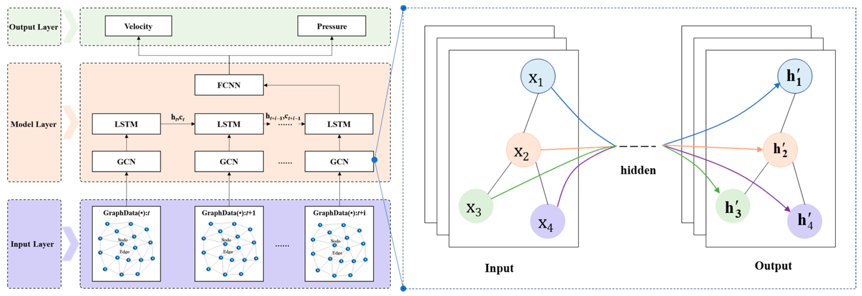
Figure 2 illustrates the layer-wise topology of the employed GCN encoder, highlighting how node-level flow features (velocity, pressure, and coordinates) were propagated through stacked spectral-based convolution layers. Each layer applied normalized neighborhood aggregation, ensuring balanced information flow across nodes of varying degrees, while the weight matrix W and nonlinear activation σ(⋅) capture complex local flow correlations. The architecture emphasizes efficient message passing across the unstructured mesh, enabling the encoder to extract essential spatial representations for subsequent LSTM-based temporal modeling.

Graph data construction: The flow field graph derived from the SUBOFF AFF-8 configuration is defined as $G=\left(v,e\right)$, where the node set v corresponds to the vertices of the unstructured grids. Each node i is associated with a feature vector:

$$x_i=\left[x_i,y_i,z_i,V_i,p_i\right]$$

(13)

where (x_i,y_i,z_i) denotes the spatial coordinates of node i, V_i represents the local velocity vector components, and p_i is the pressure at node i.

The edge set e encodes the grid topology, defined as:

$$e=\left\{\left(k_{ij},d_{ij}\right)\mid \mathrm{node} i \mathrm{and} \mathrm{node} j \mathrm{are} \mathrm{connected}\right\}$$

(14)

where k_ij is the index of the edge connecting nodes i and j and d_ij denotes the Euclidean distance between them.

Neighborhood feature aggregation: For a given node i, the output feature representation after one GCN layer is computed as:

$$h_{i,t}=\sigma \left(\sum _{j\in N_i\cup \left\{i\right\}}{\displaystyle \frac{1}{\sqrt{\mathrm{deg}\left(i\right)\mathrm{deg}\left(j\right)}}}W{h}_j\right)$$

(15)

where N_i is the set of neighboring nodes of node i, deg(i) and deg(j) are the degrees of nodes i and j, respectively, W is a shared trainable weight matrix, and σ(⋅) is a nonlinear activation function, such as ReLU.

This normalized aggregation scheme ensures that feature propagation is balanced across nodes of varying degrees.

Interlayer propagation mechanisms: For computational efficiency, the GCN layer can be expressed in matrix form as:

$${h^{\prime }}_{i,t}=\sigma \left({\widehat{D}}^{-{\displaystyle \frac{1}{2}}}\widehat{A}{\widehat{D}}^{-{\displaystyle \frac{1}{2}}}HW\right)$$

(16)

where H is the input feature matrix, ${h^{\prime }}_{i,t}$ is the output feature matrix, $\widehat{A}=A+I$ is the adjacency matrix with self-connections, and $\widehat{D}$ is the degree matrix of $\widehat{A}$.

3.2.2. GAT Encoder

GAT introduces learnable attention mechanisms into graph message passing, allowing the model to assign different importance to different neighbors based on the local flow context. In the proposed ST-GNN framework, the GAT encoder enhances spatial feature learning by emphasizing regions characterized by complex flow interactions, such as shear layers and separation zones.

Figure 3 depicts the GAT encoder architecture, showing the sequential process from input graph construction to multi-head attention-based feature propagation. Each attention head computes pairwise correlation coefficients between connected nodes, enabling adaptive weighting of neighbor contributions. By concatenating outputs from multiple heads, the model improves robustness and expressiveness in representing non-uniform flow features across the SUBOFF AFF-8 mesh.

Graph data construction: The construction of the input graph $G=\left(v,e\right)$ remains consistent with the GCN framework.

Computation of attention coefficients: For each i and its neighboring nodes j, the attention coefficient ${\alpha }_{ij}$ quantifies the strength of spatial correlation between the nodes. It is computed as:

$${\alpha }_{ij}={\displaystyle \frac{exp\left(\mathrm{LeakyReLU}\left(a^T\left[W{h}_{i,t}\parallel W{h}_{j,t}\right]\right)\right)}{{\displaystyle \sum _{k\in N_i}}exp\left(\mathrm{LeakyReLU}\left(a^T\left[W{h}_{i,t}\parallel W{h}_{k,t}\right]\right)\right)}}$$

(17)

where N_i denotes the neighborhood of node i, W is a learnable linear transformation matrix (dimensionality expansion), a is a trainable weight vector, ‖ denotes vector concatenation, and LeakyReLU is the activation function introducing nonlinearity.

Neighborhood feature aggregation: Once the attention coefficients are computed and normalized, the spatial feature representation $h_{i,t}^{\prime }$ for node iii is obtained by aggregating information from its neighbors:

$$h_{i,t}^{\prime }=\sigma \left({\displaystyle \sum }_{j\in N_i}{\alpha }_{ij}{h}_{j,t}^{\left(l\right)}\right)$$

(18)

where σ(⋅) denotes a nonlinear activation function, such as ReLU.

Multi-head attention mechanism: To enhance the model’s representation capacity and stabilize the learning process, K independent attention heads are employed. The final output is obtained by concatenating the outputs from each head:

$$h_{i,t}^{\prime }=Concat\left(h_{i,t}^1,h_{i,t}^2,\dots ,h_{i,t}^K\right)$$

(19)

3.3. Architecture of the LSTM-Based Decoder

The LSTM network is a specialized form of an RNN designed to effectively capture and retain long-range temporal dependencies by leveraging a gated memory mechanism. As illustrated in Figure 4, the LSTM employs three primary gates, including the input gate, forget gate, and output gate, to selectively filter and store sequential information over time. In this study, the LSTM was adopted as the decoder to process the sequence of latent node features $h{\prime }_{i,1}$, $h{\prime }_{i,2}$, …, $h{\prime }_{i,T}$ output by the GNN encoder. By exploiting the LSTM’s gated memory structure, the temporal evolution of the flow field was effectively learned, enabling the accurate prediction of physical quantities at the next time step, specifically the pressure p_i,T+1 and the velocity vector V_i,T+1 at node i.

The core mechanism and computational equations of the LSTM are detailed as follows:

The input gate controls the degree to which new information enters the cell state:

$$h_{i,t}^{\prime }=Concat\left(h_{i,t}^1,h_{i,t}^2,\dots ,h_{i,t}^K\right)$$

(20)

The forget gate regulates the retention or discarding of historical memory:

$$f_t=\sigma \left(W_{if}h{\prime }_{i,t}+b_{if}+W_{hf}h{\prime }_{i,t-1}+b_{hf}\right)$$

(21)

The cell state update integrates new candidate information with the prior state via gating:

$${\tilde{c}}_t=tanh\left(W_{ic}h{\prime }_{i,t}+b_{ic}+W_{hc}h{\prime }_{i,t-1}+b_{hc}\right)$$

(22)

$$c_t=f_t\odot c_{t-1}+i_t\odot {\tilde{c}}_t$$

(23)

The output gate determines the output of the current hidden state:

$$o_t=\sigma \left(W_{io}h{\prime }_{i,t}+b_{io}+W_{ho}h{\prime }_{i,t-1}+b_{ho}\right)$$

(24)

$$h{\prime }_{i,t}=o_t\odot tanh\left(c_t\right)$$

(25)

The FCNN maps the final hidden state to the target physical quantities:

$$y_i=Wh{\prime }_{i,T}+b$$

(26)

where $y_i=\left[p_i{,}_{T+1},V_i{,}_{T+1}\right]$ denotes the predicted physical variables, namely, pressure and velocity, at the next time step for node i. This formulation enables ST-GNN to capture complex spatio-temporal dependencies inherent in unsteady flow fields.

4. Case Study

To validate the ST-GNN framework’s performance, this section first details the CFD modeling of the SUBOFF AFF-8 benchmark, including data preparation, simulation setup, and experimental validation, to ensure the reliability of the training data. It then describes the ST-GNN training details and flow field prediction results.

4.1. Data Preparation for Flow Fields of the SUBOFF Benchmark

4.1.1. CFD Model Configuration and Grid Generation

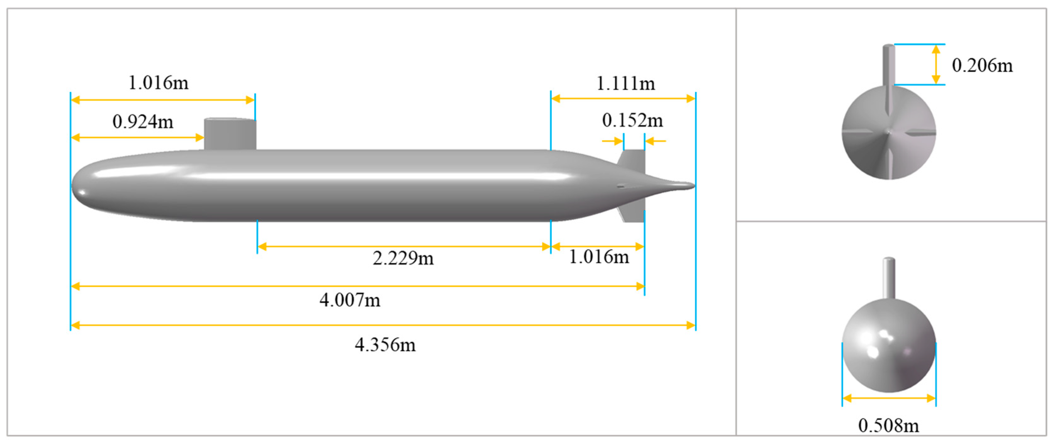
The SUBOFF AFF-8 model represents a generic axisymmetric submarine configuration, widely utilized in hydrodynamic validation studies. As illustrated in Figure 5, the model comprises a streamlined, teardrop-shaped axisymmetric hull, an ellipsoidal sail fairwater (cap), and four cruciform stern appendages. The total hull length, denoted as L, measures 4.356 m and is subdivided into three primary sections: a forebody measuring 1.016 m, a parallel midbody of 2.229 m, and an afterbody of 1.111 m. The maximum diameter (D) of the hull is 0.508 m. Positioned atop the hull is the sail fairwater (cap), characterized by an elliptical cross-section with a major-to-minor axis ratio of 2:1 and a convex elliptical dome forming its upper boundary. The sail fairwater spans 0.368 m in length and 0.460 m in height, with its leading edge located at 0.924 m and trailing edge at 1.292 m from the bow. At the stern, four NACA 0020-profile fins are symmetrically arranged in a cruciform pattern. Each fin terminates with a tip chord length of 0.152 m, and its trailing edges are located at 4.007 m from the bow.

To leverage the geometric and flow symmetry of the SUBOFF AFF-8 configuration, a half-model approach was adopted for numerical simulations, significantly reducing computational cost without compromising fidelity. The simulation domain, as depicted in Figure 6, was constructed as a rectangular prism designed to adequately capture inflow, outflow, and wake dynamics. The computational boundaries extended 0.5 L upstream and radially outward and 2 L downstream relative to the model’s length, ensuring sufficient buffer zones to minimize boundary interference effects. The inlet boundary was specified as a uniform velocity inflow, while the outlet boundary was prescribed with a zero-gauge static pressure condition. The remaining side surfaces (top, bottom, and lateral) were defined as symmetry planes. A no-slip wall condition was enforced on all wetted surfaces of the SUBOFF AFF-8 geometry. To resolve near-wall behavior and complex flow separations, the computational domain was discretized using a hybrid grid strategy, consisting of cut-cell Cartesian grids in the far-field and prismatic boundary-layer elements adjacent to solid surfaces. Furthermore, volume-controlled local grid refinement was applied in regions exhibiting high flow gradients, including the hull–sail junction, stern appendages, and near-wake region.

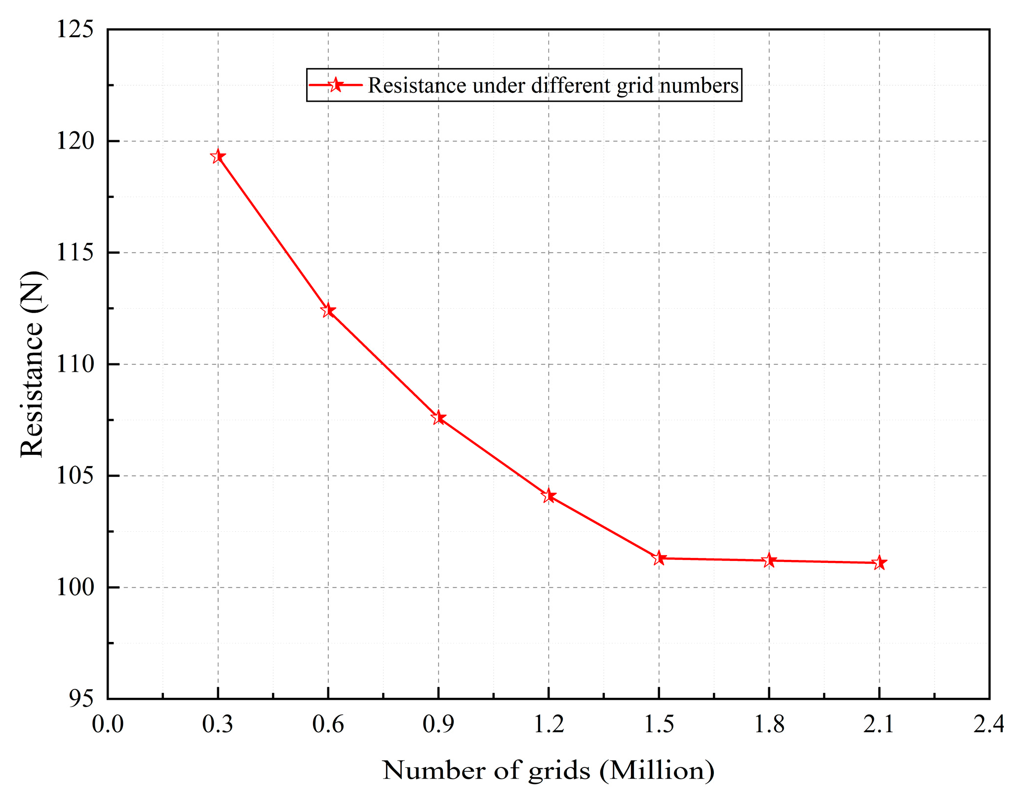
To verify spatial discretization independence, a systematic grid sensitivity study was conducted. Seven progressively refined computational grids were evaluated, spanning from 0.3 million to 2.1 million cells in 0.3 million cell increments. Figure 7 illustrates the variation in resistance with grid refinement. The results demonstrated that grid convergence is achieved at 1.5 million cells, where further refinement to 1.8 million and 2.1 million cells yielded negligible resistance variation (<0.1%). At this optimal resolution, the computed resistance exhibited excellent quantitative agreement with experimental data, showing a relative error of −0.98%. Consequently, a grid resolution of 1.5 million cells was established, achieving an optimal trade-off between computational accuracy and efficiency.

4.1.2. CFD Solution and Experimental Validation

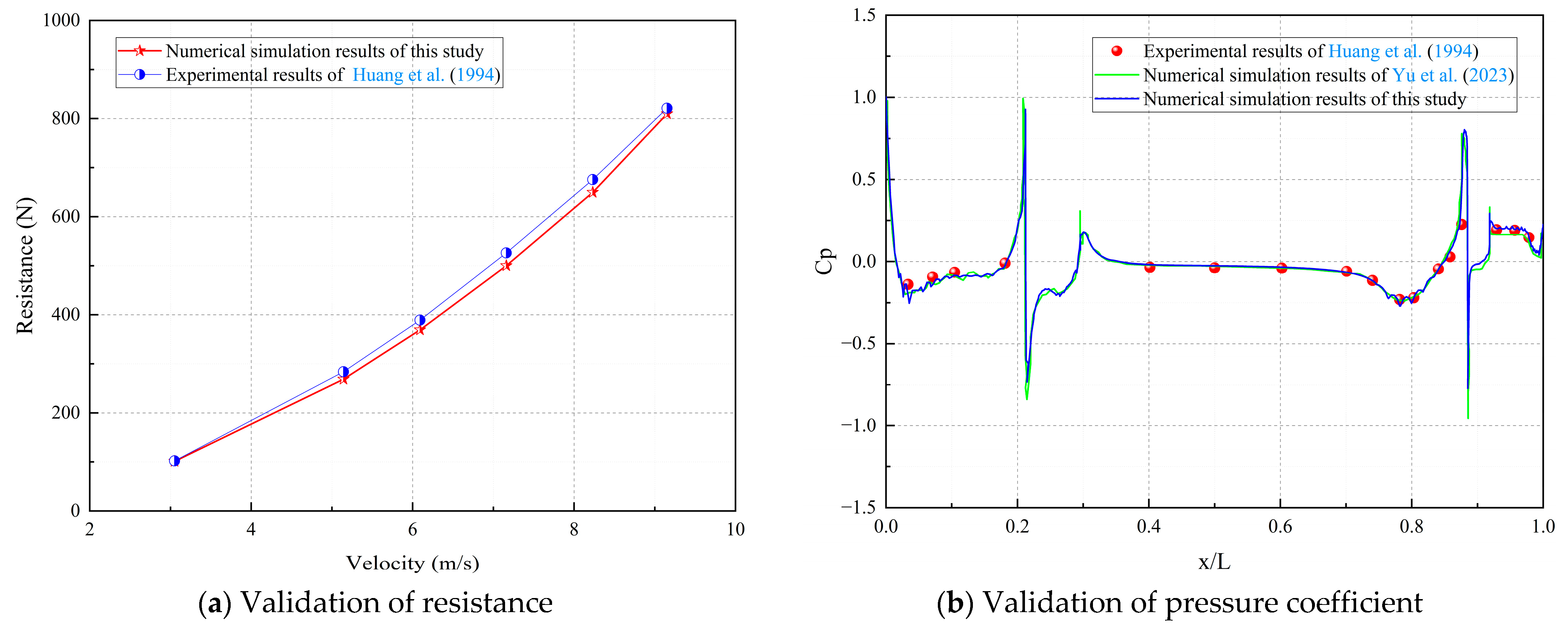
The governing equations for incompressible fluid flow were discretized using the finite volume method (FVM), a robust and widely adopted approach in computational fluid dynamics. To resolve the pressure–velocity coupling, the SIMPLE algorithm was employed, ensuring stable and efficient convergence. A uniform time step of 0.004 s was employed, with 10 inner iterations per time step to enhance temporal resolution. The simulation was conducted until a total physical time of 4 s was achieved. Details of the computational setup and boundary conditions are summarized in

Table 1. Computational cases for the CFD simulation of SUBOFF AFF-8.

Cases	Velocity (m/s)	Reynolds Number	Experimental Resistance (N)	Simulation Resistance (N)	Relative Error (%)
Case 1	3.051	1.24 × 107	102.3	101.3	−0.98
Case 2	5.144	2.095 × 107	283.8	269.7	−4.97
Case 3	6.091	2.481 × 107	389.2	371.2	−4.62
Case 4	7.161	2.917 × 107	526.2	500.6	−4.86
Case 5	8.231	3.354 × 107	675.6	649.6	−3.85
Case 6	9.152	3.769 × 107	821.1	809.9	−1.36

. To evaluate the accuracy and reliability of the numerical framework, the simulation results were quantitatively compared with experimental measurements reported by Huang et al. (1994) and computational results presented by Yu et al. (2023) [29,30]. As illustrated in Table 1 and Figure 8a, the predicted hydrodynamic resistance shows excellent agreement with the experimental data, with minimum, maximum, and mean relative errors of 0.98%, 4.97%, and 3.44%, respectively. In addition, Figure 8b presents a comparison of the dimensionless pressure coefficient (Cp) along the hull, where the numerical results closely replicate the trends, peaks, and spatial distribution observed in the experimental measurements. These findings are also in good agreement with the results of Yu et al. (2023), further corroborating the robustness of the computational model [30]. Overall, the validation demonstrates that the developed numerical model provides high predictive accuracy, rendering it suitable for generating reliable, high-resolution datasets to support the training and evaluation of advanced spatio-temporal graph based deep learning models, such as ST-GNN.

4.2. Flow Field Prediction Case Study Using ST-GNN

4.2.1. Hyperparameter Setting and Training

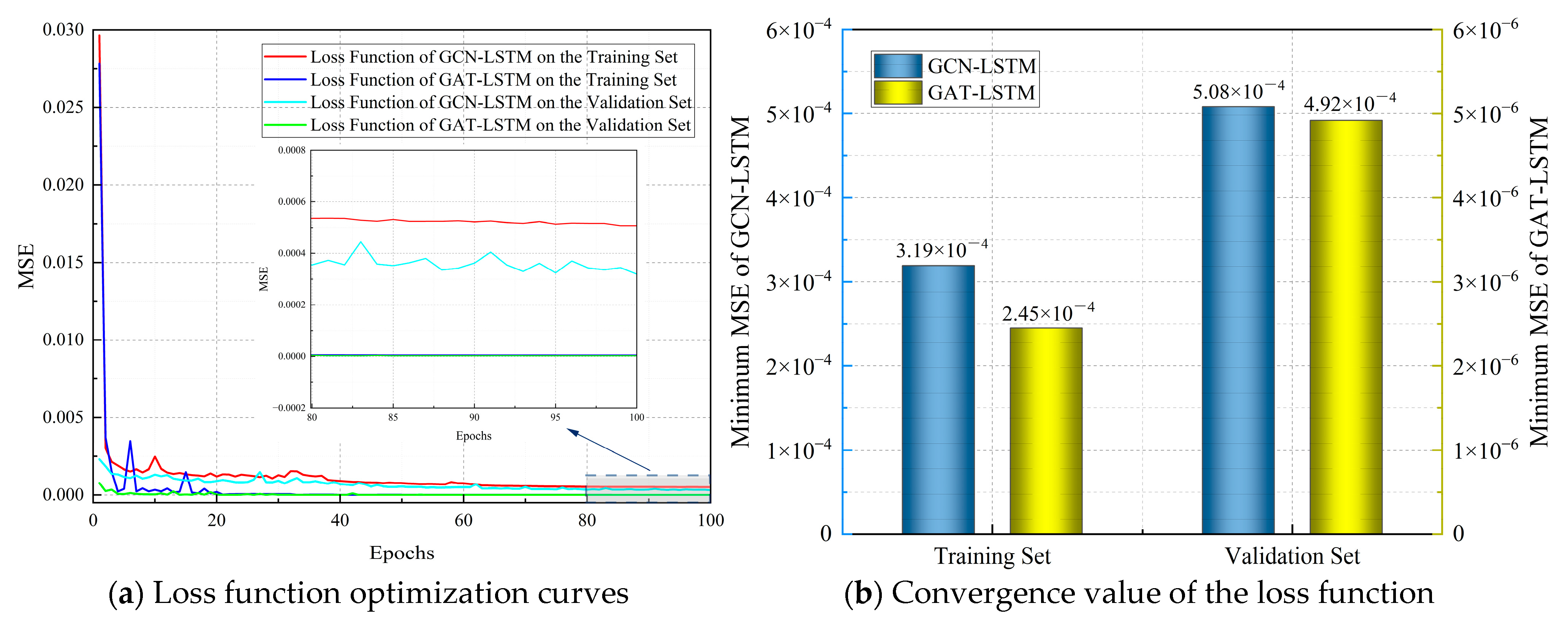
Two variants of the proposed ST-GNN architecture, namely, GCN-LSTM and GAT-LSTM, were trained and iteratively optimized using the SUBOFF AFF-8 flow field dataset, which was derived from the aforementioned CFD simulations and sampled across 1000 discrete time step indices (n_t) for case 1. The graph-structured dataset was partitioned at a ratio of 8:1:1 into training, validation, and test sets. Specifically, data corresponding to the first 800 time steps were allocated for training, with 800 to 899 for validation, and the remaining 100 time steps for testing. Z-score normalization was applied to preprocess the input data, aiming to eliminate the impact of dimensional differences during model training. The GNN components (including both the GCN and GAT) and the LSTM module were configured with 10 and 2 layers, respectively, each with a hidden dimensionality of 128. A temporal sliding window of size 10 was employed, and the batch size was set to 3. The initial learning rate was set to 0.001 and adaptively adjusted during training using the ReduceLROnPlateau scheduler. Model optimization was performed using the Adam optimizer, with L2 regularization and early stopping incorporated to mitigate overfitting. The ReLU activation function was utilized, and the Mean Squared Error (MSE) was adopted as the loss function. As depicted in Figure 9a, after 100 training epochs, the loss curves on both the training and validation sets exhibited convergence and stabilization. Furthermore, as shown in Figure 9b, the MSE values for the GCN-LSTM and GAT-LSTM models converged to approximately 3.19 × 10⁻⁴ and 2.45 × 10⁻⁶ on the training set, and to 5.08 × 10⁻⁴ and 4.92 × 10⁻⁶ on the validation set, respectively.

4.2.2. Quantitative Validation of Prediction Results

Following the completion of model training, flow field predictions were performed using a temporal sliding window approach on the test set. Specifically, the models were initialized with graph-structured data corresponding to 10 consecutive time steps (from 900 to 909), enabling the prediction of the flow field at 910. Subsequently, the window was advanced by one step, using data from n_t = 901 to n_t = 910 to predict n_t = 911. This autoregressive procedure was repeated iteratively, allowing the models to generate sequential predictions across the entire future temporal domain. Figure 10 and Figure 11 illustrate the predicted velocity and pressure fields at n_t = 950, as predicted by the GCN-LSTM and GAT-LSTM models for the SUBOFF AFF-8 dataset. The predicted flow field distributions exhibited strong agreement with those obtained from high-fidelity CFD simulations, reflecting both spatial coherence and physical plausibility. Quantitatively, the mean relative errors of the GCN-LSTM model in predicting the velocity and pressure fields were 3.48% and 1.79%, respectively, while the GAT-LSTM model achieved slightly lower errors of 0.93% and 0.67%, respectively. These results affirm the effectiveness and robustness of both ST-GNN variants in accurately modeling the spatio-temporal evolution of flow fields on unstructured grids.

5. Results and Discussion

This section analyzes the ST-GNN prediction results from three perspectives: visual flow field contours, statistical error evolution, and pressure coefficient (Cp) accuracy. The computational efficiency between ST-GNN and CFD is benchmarked to highlight the practical advantages of the former.

5.1. Visual Analysis of Predicted Flow Field Contours

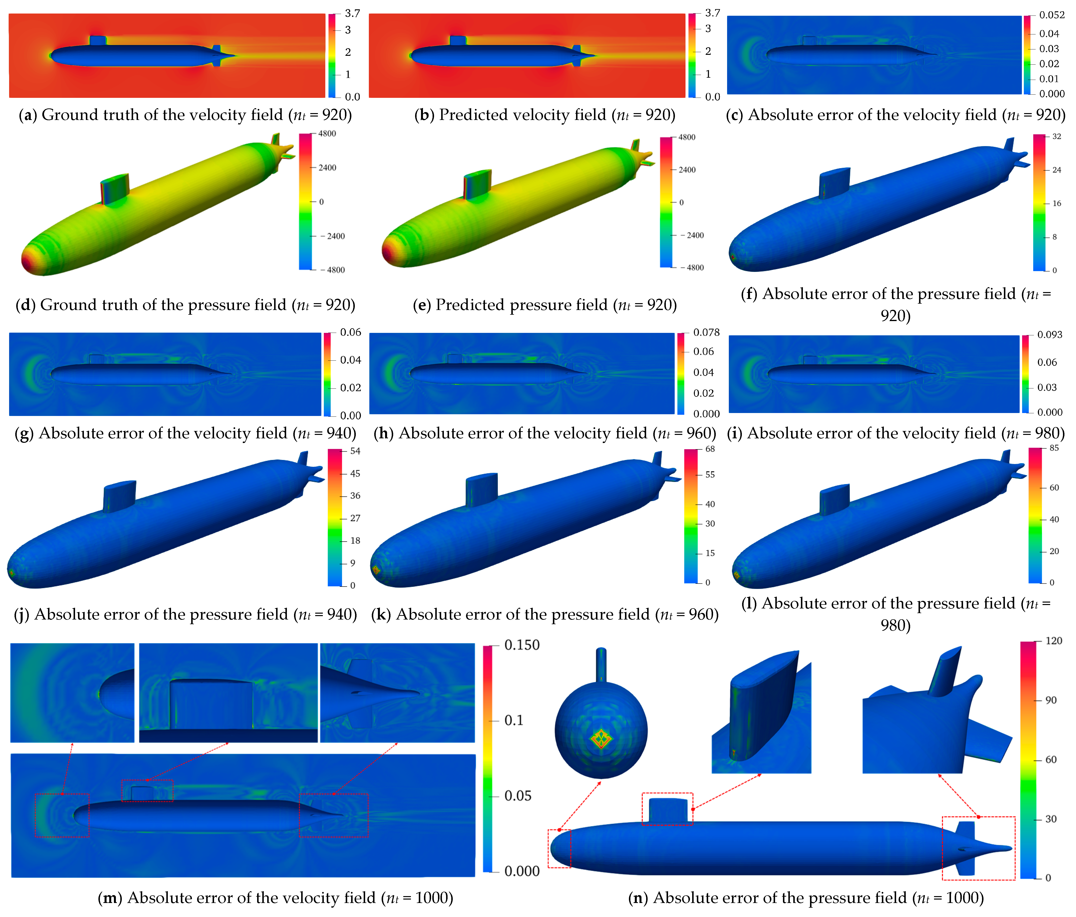
A rigorous assessment of the temporal generalizability of the GCN-LSTM and GAT-LSTM architectures was conducted for velocity/pressure field predictions around the SUBOFF AFF-8 hull. Contour visualizations (Figure 12 and Figure 13) across five strategically selected time step indices (n_t = 920, 940, 960, 980, 1000, corresponding to physical times of 3.68 s, 3.76 s, 3.84 s, 3.92 s, 4.00 s) revealed a pronounced progressive accumulation of prediction errors in both models as time advances. This phenomenon arises from the autoregressive inference paradigm, wherein each sequential prediction depends recursively on the preceding output. Consequently, initial minor inaccuracies propagate and amplify through the prediction horizon, culminating in a cascade “snowball” effect that progressively diverges from the true spatio-temporal evolution of the flow field. This mechanistic insight underscores a core challenge inherent to data-driven approaches for long-term unsteady flow modeling.

The comparative evaluation demonstrated a consistent and statistically significant performance advantage of GAT-LSTM over GCN-LSTM across the entire temporal domain for both velocity and pressure predictions. This superiority is particularly evident within critical flow regions characterized by steep gradients, such as shear layers and flow separation zones. The enhanced fidelity of GAT-LSTM is attributable to its integrated graph attention mechanism, which transcends the limitations of fixed, topology-defined neighborhood aggregation inherent to GCNs. By dynamically computing attention coefficients between nodes, GAT-LSTM adaptively prioritizes and weights the most influential local flow features. This enables the model to selectively focus computational resources on resolving strongly nonlinear phenomena, including vortical structures and separation dynamics, thereby achieving a more precise characterization of localized structural discontinuities and significantly boosting predictive robustness in complex flow regimes.

The spatial distribution of prediction accuracy exhibited marked heterogeneity, strongly correlated with geometric complexity. Regions featuring abrupt geometric discontinuities, notably the bow stagnation point, the conning tower–hull junction, and stern appendages, such as the rudder and propeller, suffered significantly elevated prediction errors in both models compared to hydrodynamically smooth hull sections. This spatial error concentration arises directly from the intense physical gradients (velocity, pressure) induced by sharp geometric features and high curvature. These topologically complex zones invariably host intricate flow physics, encompassing sustained flow separation, coherent vortex shedding, and adverse pressure gradients, where field variables manifest highly nonlinear, transient behavior. Critically, while GAT-LSTM maintains an overall accuracy advantage through its attention mechanism, neither model fully resolves the intricate transient dynamics generated by severe geometric forcing. The persistent error elevation in these regions highlights a fundamental limitation of current spatio-temporal graph networks in capturing geometry-driven flow nonlinearities, thereby establishing an essential trajectory for future model refinement.

5.2. Statistical Analysis of Prediction Relative Errors

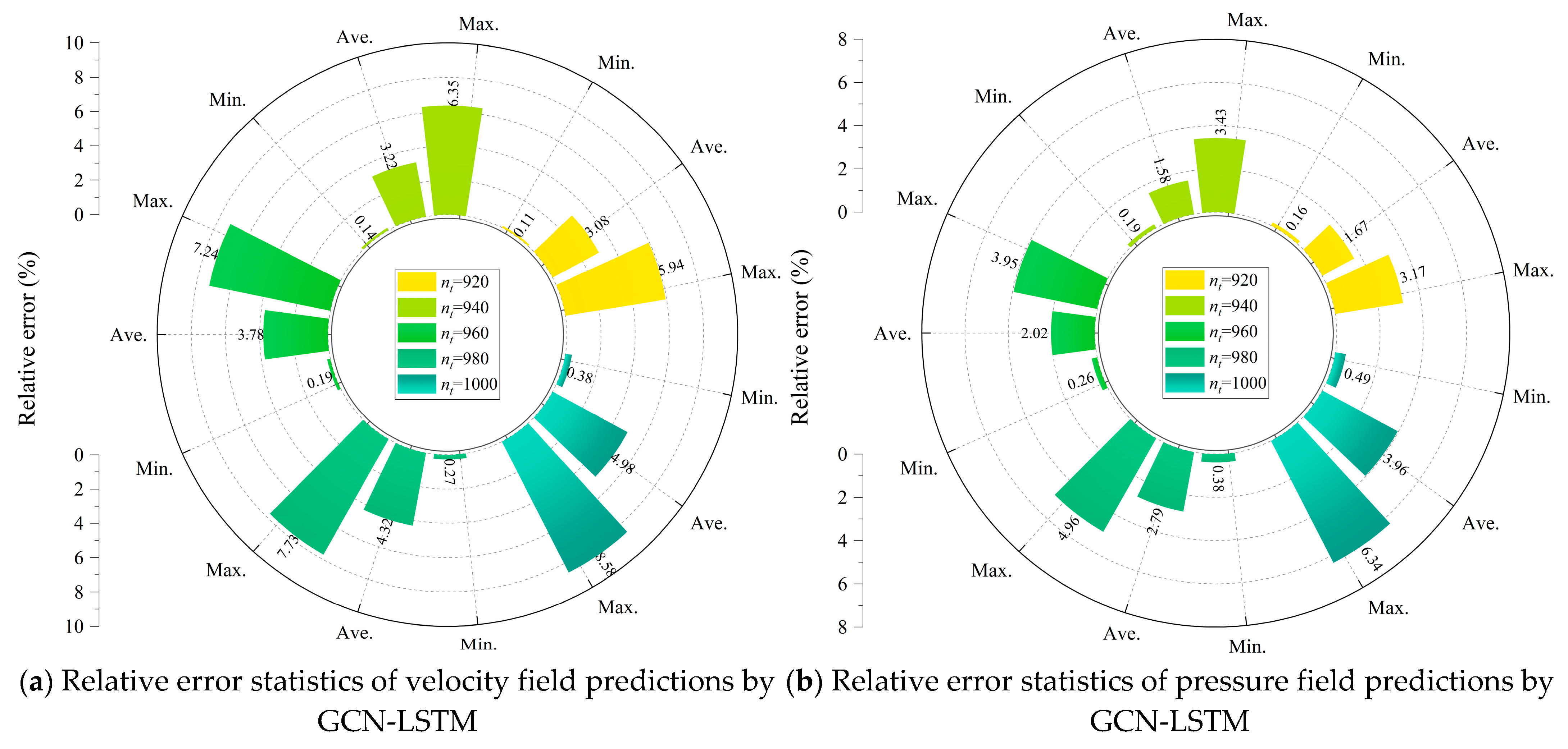
This subsection presents a rigorous quantitative assessment of the temporal evolution characteristics of relative errors in the flow field predictions obtained from the GCN-LSTM and GAT-LSTM models, with particular attention to the prediction horizon ranging from n_t = 920 to n_t = 1000 for the SUBOFF AFF-8 hydrodynamic configuration. For the GCN-LSTM model, a distinct and consistent upward trend was observed in the relative errors associated with both the velocity and pressure field predictions over time. As depicted in Figure 14a,b, the maximum relative error in the velocity field increased from 5.94% at n_t = 920 to 8.58% at n_t = 1000, representing a notable 44.4% increase. In parallel, the average relative error rose from 3.08% to 4.98%, constituting a substantial 61.7% escalation. The degradation in prediction accuracy was even more pronounced in the pressure field: the maximum relative error nearly doubled, surging from 3.17% to 6.34%, an increase of 99.7%, while the average relative error increased by 137.1%, climbing from 1.67% to 3.96%. These trends provide quantitative evidence of the error compounding inherent in autoregressive inference, which becomes especially significant in geometrically complex regions where capturing fine-scale flow structures proves more difficult.

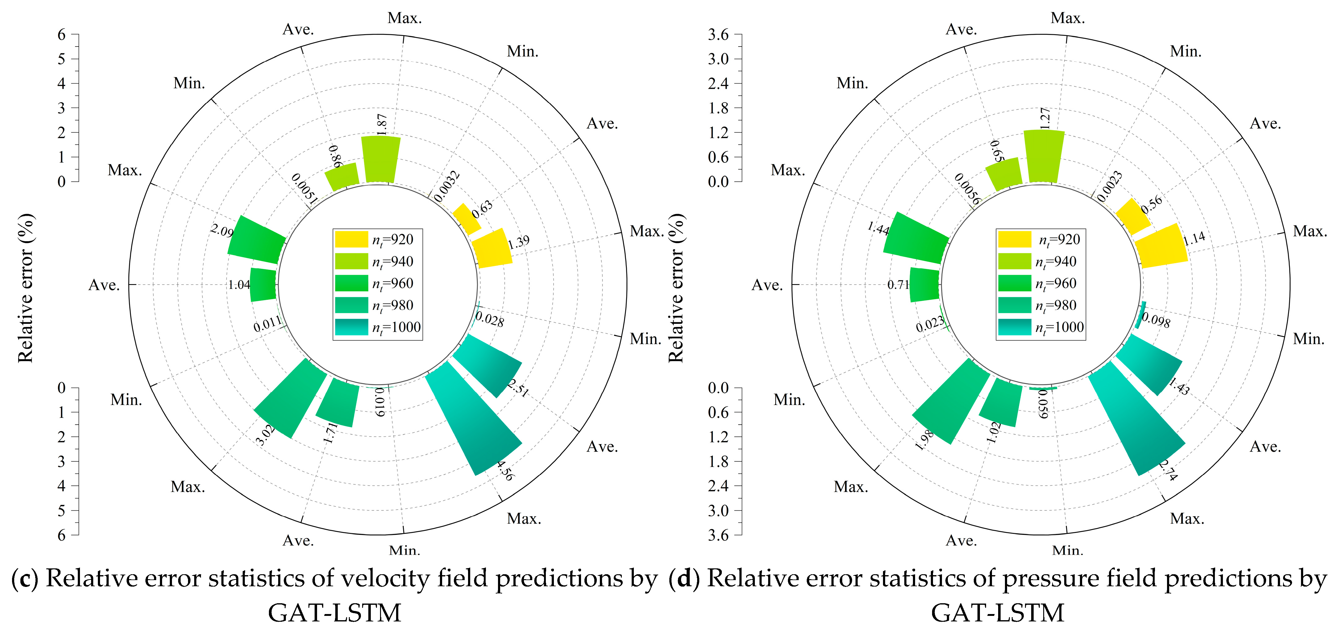
In contrast, the GAT-LSTM model demonstrated a strikingly enhanced capacity for controlling error accumulation. As illustrated in Figure 14c,d, the maximum velocity field error grew from a relatively low 1.39% at n_t = 920 to 4.56% at n_t = 1000, corresponding to a 228.0% increase, while the average error increased from 0.63% to 2.51%, a numerically large 298.4% rise. Although these relative percentage increases appear substantial, they must be interpreted against the backdrop of significantly lower initial error magnitudes. For instance, the initial maximum velocity field error for GAT-LSTM is only 23.4% of that for GCN-LSTM. In the pressure field, the maximum and average relative errors increased from 1.14% to 2.74% and 0.56% to 1.43%, reflecting increases of 140.4% and 155.4%, respectively. Nonetheless, across the entire prediction window, GAT-LSTM maintained consistently lower absolute errors, attesting to its greater temporal stability and predictive reliability.

A direct comparison at n_t = 1000 reinforces the superior generalization performance of GAT-LSTM. At this time point, the model achieved reductions of 49.6% and 63.9% in the average relative errors of the velocity and pressure fields, respectively, compared to GCN-LSTM. Furthermore, the maximum relative errors remained well-constrained within 4.56% for the velocity field and 2.74% for the pressure field. These results clearly underscore the efficacy of incorporating attention mechanisms within the recurrent graph-based framework. The graph attention layers appear to effectively mitigate error propagation across time steps, particularly in scenarios where spatial and temporal dynamics interact nonlinearly, as is often the case in turbulent or complex flow regimes.

In summary, both the GCN-LSTM and GAT-LSTM models maintained average relative errors below 5% throughout extended prediction intervals, thereby demonstrating their promising potential for long-term flow field forecasting on unstructured grids. Nevertheless, the GAT-LSTM architecture exhibited a clear advantage, not only in error minimization but also in generalization robustness, particularly in handling intricate flow patterns and challenging boundary conditions. This confirms the significant practical merit of attention-enhanced spatio-temporal models in advancing the frontier of data-driven fluid dynamics.

5.3. Analysis of Pressure Coefficient Prediction Results

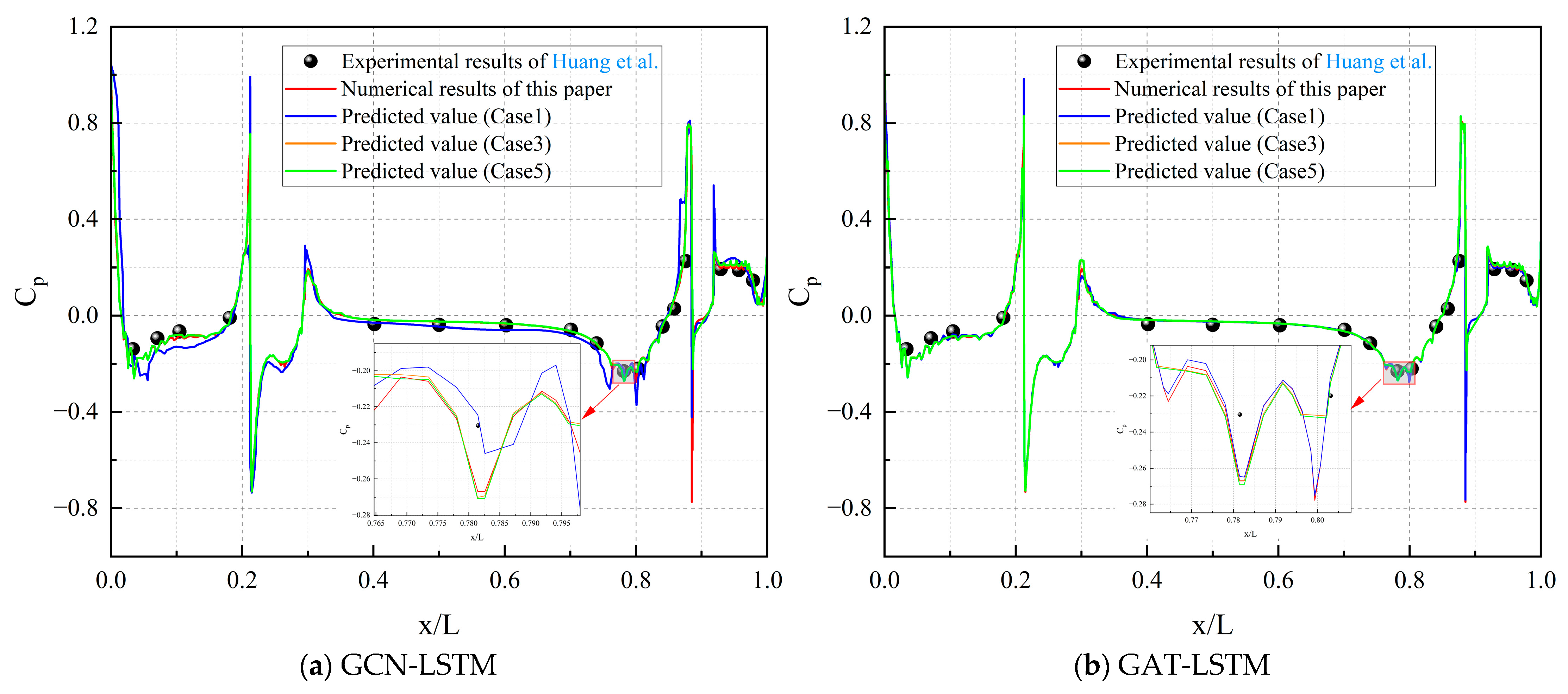
This subsection presents a rigorous comparative assessment of the Cp prediction performance between the GCN-LSTM and GAT-LSTM models for the SUBOFF AFF-8 hull configuration, leveraging the diagnostic insights from Figure 15. As depicted in Figure 15a, the GCN-LSTM model initially captured the overarching spatio-temporal trend of the Cp distribution at early stages (e.g., n_t = 920). However, when progressing to n_t = 1000, progressive deviations emerged. Specifically, the model exhibited subtle inaccuracies in locating peak pressures within critical regions: minor shifts manifested at high-pressure zones (e.g., the bow stagnation point) and low-pressure regions (e.g., aft of the sail and near the rudder). Additionally, differences in amplitudes were observed, particularly an underestimation of negative pressure peaks in separation-sensitive zones.

In stark contrast, the GAT-LSTM model demonstrated exceptional spatio-temporal predictive fidelity across all time steps, as illustrated in Figure 15b. Its Cp curves exhibited near-perfect quantitative and qualitative alignment with ground-truth data, maintaining remarkable precision in shape, peak localization, and amplitude magnitude. Key hydrodynamic regions, including the bow stagnation point, sail junction, and stern appendages, showed no measurable degradation in curve smoothness, peak integrity, or spatio-temporal coherence.

Collectively, these results underscore a statistically significant performance differential between the architectures. The GAT-LSTM’s attention mechanism enabled near-ideal Cp replication, validating its robustness for long-term fluid–structure interaction forecasting. Conversely, the GCN-LSTM’s accuracy diminished monotonically over time, particularly in resolving critical peak features, highlighting limitations in capturing complex boundary layer transition and separation dynamics. This performance divergence further accentuates the transformative role of graph attention mechanisms in advancing the accuracy of high-fidelity hydrodynamic simulations for engineering-relevant configurations.

To further assess the model’s generalizability across varying flow conditions, we expanded the evaluation to include three representative cases from Table 1: Case 1 (Re = 1.24 × 10⁷), Case 3 (Re = 2.481 × 10⁷), and Case 5 (Re = 3.354 × 10⁷). While training and validation were primarily conducted on Case 1, the models’ predictions of pressure coefficients (Cp) under these diverse Reynolds numbers and boundary conditions were systematically validated against both experimental data and high-fidelity CFD simulations. As shown in Figure 16a for GCN-LSTM and Figure 16b for GAT-LSTM, both models maintain strong alignment with the ground-truth Cp distributions across the tested cases, with GAT-LSTM again exhibiting superior fidelity in capturing peak locations and amplitudes, especially in regions influenced by higher Reynolds numbers where flow separation and turbulence intensify. These results confirm robust performance under extrapolated operating conditions, with minimal degradation in accuracy, thereby strengthening the empirical evidence for the models’ generalizability and practical applicability in varied hydrodynamic scenarios.

5.4. Solving Efficiency Analysis of ST-GNN and CFD

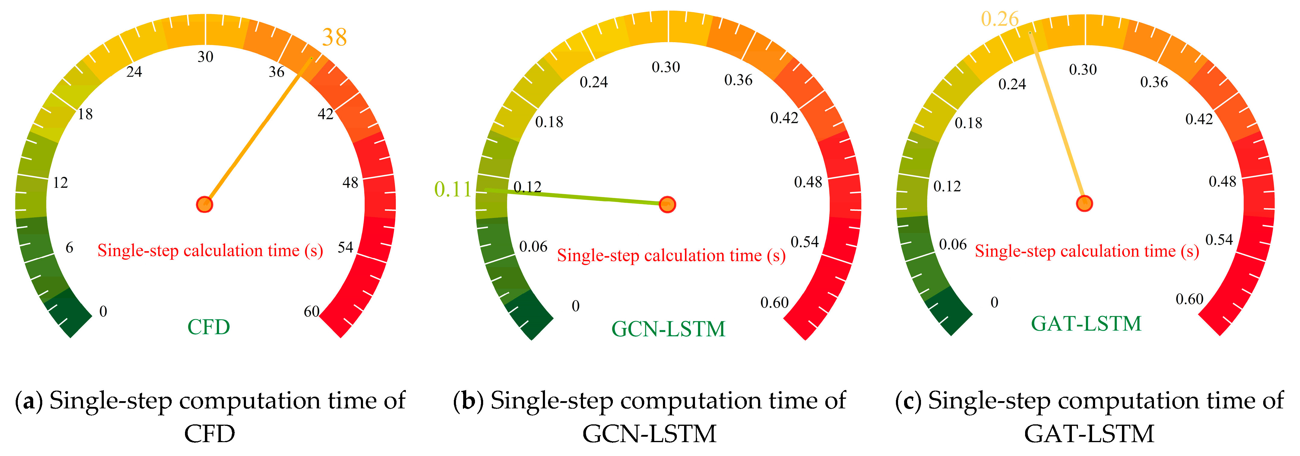
As illustrated in Figure 17, the single-step solution time of the CFD simulation for the SUBOFF AFF-8 model reached 38 s, with computational bottlenecks primarily arising from the iterative solution of partial differential equations and complex discretization of the computational domain. Specifically, CFD employed the finite volume method to spatially discretize governing equations and relied on the SIMPLE iterative algorithm to solve pressure–velocity coupling at each time step, leading to prolonged computation. In contrast, the ST-GNN models (GCN-LSTM and GAT-LSTM) achieved remarkable inference efficiency, with single-step prediction times of merely 0.11 s and 0.26 s, respectively, achieving approximately 350× and 150× speedup over the CFD simulations. This dramatic acceleration is attributable to the parametric mapping capability inherent in GNNs, which, once trained, predict spatio-temporal flow-field evolution through a single, highly efficient forward propagation, thereby completely obviating the need for iterative equation solving. Comparing the two ST-GNN variants, GCN-LSTM exhibited marginally higher efficiency than GAT-LSTM. The GCN performs graph convolution with a fixed adjacency matrix, featuring a computational complexity of O(N) (where N is the number of nodes), whereas GAT introduces attention mechanisms that require dynamic calculation of adjacency weights for each node. This incurs additional computational overhead of O(N × K) (with K denoting the average number of neighbors, and K < N), contributing to a longer execution time for GAT. Collectively, these findings underscore the substantial potential of ST-GNN frameworks for real-time or large-scale flow-field analyses where rapid inference is mission-critical.

6. Conclusions

This study proposed a novel ST-GNN framework for predicting unsteady flow fields on unstructured grids. By integrating graph encoders, specifically a GCN and GAT, with LSTM decoders, the model effectively captures both spatial topology and temporal dynamics in complex fluid systems. Based on evaluation using the SUBOFF AFF 8 test case, the following conclusions are drawn:

(1) The ST-GNN framework demonstrates strong capability in modeling the spatio-temporal evolution of unsteady flow fields. GAT-LSTM outperforms GCN-LSTM by leveraging an adaptive graph attention mechanism that focuses on critical flow regions with high gradients, such as shear layers and separation zones, leading to more accurate resolution of fine-scale flow features.

(2) Although both ST-GNN variants exhibit gradually increasing prediction errors over time, due to the autoregressive inference process, their overall error levels remain low. GAT-LSTM shows notably better control over error propagation, achieving significantly lower average relative errors in velocity and pressure predictions by the final time step.

(3) The ST-GNN models provide a substantial improvement in computational efficiency compared to traditional CFD solvers. By using pre-trained parametric mappings rather than solving PDEs iteratively, both variants reduce computation time per step by two orders of magnitude. While GCN-LSTM is slightly faster, GAT-LSTM offers superior accuracy, making it more suitable for precision-sensitive applications, such as real-time flow analysis and design optimization.

(4) Both models encounter challenges near abrupt geometric features, for example, bow stagnation points and stern appendages, where strong nonlinearities occur due to flow separation and adverse pressure gradients. GAT-LSTM still achieves better accuracy in these regions, constraining maximum errors to lower levels, which suggests its stronger capability in handling geometry-induced flow complexities.

The ST-GNN framework, particularly GAT-LSTM, offers a promising solution for real-time simulation and engineering applications in complex flow fields. To further enhance accuracy in capturing local flow complexities, future work will incorporate physical constraints, such as Navier–Stokes equation terms, into the loss function. This physics-informed approach aims to strengthen adherence to fluid dynamics principles, improving predictive performance in challenging flow scenarios.

References

1. Brunton, S.L.; Noack, B.R.; Koumoutsakos, P. Machine learning for fluid mechanics. Annu. Rev. Fluid Mech. 2020, 52, 477–508. [Google Scholar] [CrossRef]
2. Wang, H.; Cao, Y.; Huang, Z.; Liu, Y.; Hu, P.; Luo, X.; Song, Z.; Zhao, W.; Liu, J.; Sun, J.; et al. Recent advances on machine learning for computational fluid dynamics: A survey. arXiv 2024, arXiv:2408.12171. [Google Scholar] [CrossRef]
3. Chen, X.; Wang, Z.; Deng, L.; Yan, J.; Gong, C.; Yang, B.; Wang, Q.; Zhang, Q.; Yang, L.; Pang, Y.; et al. Towards a new paradigm in intelligence-driven computational fluid dynamics simulations. Eng. Appl. Comput. Fluid Mech. 2024, 18, 2407005. [Google Scholar] [CrossRef]
4. Dosovitskiy, A.; Fischer, P.; Ilg, E.; Hausser, P.; Hazirbas, C.; Golkov, V.; Smagt, P.; Cremers, D.; Brox, T. Flownet: Learning optical flow with convolutional networks. In Proceedings of the IEEE International Conference on Computer Vision, Xi’an, China, 18–20 September 2015; pp. 2758–2766. [Google Scholar]
5. Bhatnagar, S.; Afshar, Y.; Pan, S.; Duraisamy, K.; Kaushik, S. Prediction of aerodynamic flow fields using convolutional neural networks. Comput. Mech. 2019, 64, 525–545. [Google Scholar] [CrossRef]
6. Zhang, M.; Cao, J. Flow Field Prediction of Variable Geometry using a Novel Deep CNN Model with Dual-Feature of Flow Regions. In Proceedings of the 43rd Chinese Control Conference, Kunming, China, 28–31 July 2024; pp. 7486–7491. [Google Scholar]
7. Halder, R.; Damodaran, M.; Khoo, B.C. Deep learning based reduced order model for airfoil-gust and aeroelastic interaction. AIAA J. 2020, 58, 4304–4321. [Google Scholar] [CrossRef]
8. Mohan, A.T.; Gaitonde, D.V. A deep learning based approach to reduced order modeling for turbulent flow control using LSTM neural networks. arXiv 2018, arXiv:1804.09269. [Google Scholar] [CrossRef]
9. Jin, X.; Laima, S.; Chen, W.L.; Li, H. Time-resolved reconstruction of flow field around a circular cylinder by recurrent neural networks based on non-time-resolved particle image velocimetry measurements. Exp. Fluids 2020, 61, 114. [Google Scholar] [CrossRef]
10. Hasegawa, K.; Fukami, K.; Murata, T.; Fukagata, K. CNN-LSTM based reduced order modeling of two-dimensional unsteady flows around a circular cylinder at different Reynolds numbers. Fluid Dyn. Res. 2020, 52, 065501. [Google Scholar] [CrossRef]
11. Portal-Porras, K.; Fernandez-Gamiz, U.; Zulueta, E.; Irigaray, O.; Garcia-Fernandez, R. Hybrid LSTM + CNN architecture for unsteady flow prediction. Mater. Today Commun. 2023, 35, 106281. [Google Scholar] [CrossRef]
12. Raissi, M.; Perdikaris, P.; Karniadakis, G.E. Physics-informed neural networks: A deep learning framework for solving forward and inverse problems involving nonlinear partial differential equations. J. Comput. Phys. 2019, 378, 686–707. [Google Scholar] [CrossRef]
13. Meng, X.; Li, Z.; Zhang, D.; Karniadakis, G.E. PPINN: Parareal physics-informed neural network for time-dependent PDEs. Comput. Methods Appl. Mech. Eng. 2020, 370, 113250. [Google Scholar] [CrossRef]
14. Chu, X.; Guo, W.; Wu, T.; Zhou, Y.; Zhang, Y.; Cai, S.; Yang, G. Flow reconstruction over a SUBOFF model based on LBM-generated data and physics-informed neural networks. Ocean Eng. 2024, 308, 118250. [Google Scholar] [CrossRef]
15. Pfaff, T.; Fortunato, M.; Sanchez-Gonzalez, A.; Battaglia, P. Learning mesh-based simulation with graph networks. In Proceedings of the International Conference on Learning Representations, Addis Ababa, Ethiopia, 26–30 April 2020. [Google Scholar]
16. Fortunato, M.; Pfaff, T.; Wirnsberger, P.; Pritzel, A.; Battaglia, P. Multiscale meshgraphnets. arXiv 2022, arXiv:2210.00612. [Google Scholar] [CrossRef]
17. Yang, Z.; Dong, Y.; Deng, X.; Zhang, L. AMGNET: Multi-scale graph neural networks for flow field prediction. Connect. Sci. 2022, 34, 2500–2519. [Google Scholar] [CrossRef]
18. Li, T.; Zou, S.; Chang, X.; Zhang, L.; Deng, X. Predicting unsteady incompressible fluid dynamics with finite volume informed neural network. Phys. Fluids. 2024, 36, 043601. [Google Scholar] [CrossRef]
19. Li, T.; Zou, Y.; Zou, S.; Chang, X.; Zhang, L.; Deng, X. A fully differentiable gnn-based pde solver: With applications to poisson and navier-stokes equations. arXiv 2024, arXiv:2405.04466. [Google Scholar]
20. Zou, Y.; Li, T.; Lu, L.; Wang, J.; Zou, S.; Zhang, L.; Deng, X. Finite-difference-informed graph network for solving steady-state incompressible flows on block-structured grids. Phys. Fluids. 2024, 36, 103608. [Google Scholar] [CrossRef]
21. Ogoke, F.; Meidani, K.; Hashemi, A.; Farimani, A.B. Graph convolutional networks applied to unstructured flow field data. Mach. Learn. Sci. Technol. 2021, 2, 045020. [Google Scholar] [CrossRef]
22. Peng, J.Z.; Wang, Y.Z.; Chen, S.; Chen, Z.H.; Wu, W.T.; Aubry, N. Grid adaptive reduced-order model of fluid flow based on graph convolutional neural network. Phys. Fluids. 2022, 34, 087121. [Google Scholar] [CrossRef]
23. Liu, Q.; Zhu, W.; Ma, F.; Jia, X.; Gao, Y.; Wen, J. Graph attention network-based fluid simulation model. AIP Adv. 2022, 12, 095114. [Google Scholar] [CrossRef]
24. Covoni, G.; Montomoli, F.; Tagarielli, V.L.; Bisio, V.; Rossin, S.; Ruggiero, M. Application of graph neural networks to predict explosion-induced transient flow. Adv. Model. Simul. Eng. Sci. 2024, 11, 18. [Google Scholar] [CrossRef]
25. Hadizadeh, F.; Mallik, W.; Jaiman, R.K. A graph neural network surrogate model for multi-objective fluid-acoustic shape optimization. arXiv 2024, arXiv:2412.16817. [Google Scholar] [CrossRef]
26. Gao, H.; Zhuang, L.; Li, C.; Qian, W.; Dong, J.; Liu, L.; Liu, J. Fast prediction of three-dimensional indoor flow fields by a reduced dimensional deep-learning approach. Build. Environ. 2025, 270, 112517. [Google Scholar] [CrossRef]
27. Chen, H.Y.; Xue, L.; Liu, L.; Zou, G.F.; Han, J.X.; Dong, Y.B.; Cong, M.Z.; Liu, Y.T.; Hosseini-Nasab, S.M. Physics-informed graph neural network for predicting fluid flow in porous media. Pet. Sci. 2025. [Google Scholar] [CrossRef]
28. Cheng, S.; Bocquet, M.; Ding, W.; Finn, T.S.; Fu, R.; Fu, J.; Guo, Y.; Johnson, E.; Li, S.; Liu, C.; et al. Machine learning for modelling unstructured grid data in computational physics: A review. Inf. Fusion 2025, 123, 103255. [Google Scholar] [CrossRef]
29. Huang, T.; Liu, H.L. Measurements of Flows over an Axisymmetric Body with Various Appendages in a Wind Tunnel: The DARPA SUBOFF Experimental Program. In Proceedings of the 19th Symposium on Naval Hydrodynamics, Seoul, Republic of Korea, 23–28 August 1992; National Academy Press: Washington, DC, USA, 1994; pp. 321–346. [Google Scholar]
30. Yu, L.; Yang, C.; Zhao, W.; Wan, D. Numerical Prediction Study of Nonlinear Hydrodynamic Noise for SUBOFF Submarine. Shipbuild. China 2023, 64, 229–239. [Google Scholar]
Figure 1. Architecture of the Spatio-temporal Graph Neural Network (ST-GNN) framework, which includes a Graph Neural Network encoder (GCN or GAT) that receives SUBOFF graph structure data and captures spatial dependencies through message passing, a Long Short-Term Memory network (LSTM) decoder that models temporal evolution via gated mechanisms, and a fully connected neural network (FCNN) for reconstructing physical quantities such as velocity and pressure fields.
Jmse 13 01647 g001
Figure 2. Topology of the GCN.
Jmse 13 01647 g002
Figure 3. Topology of GAT.
Jmse 13 01647 g003
Figure 4. Topology of the LSTM.
Jmse 13 01647 g004
Figure 5. Schematic diagram of geometric modeling.
Jmse 13 01647 g005
Figure 6. Schematic diagram of the computational grids.
Jmse 13 01647 g006
Figure 7. Grid convergence analysis.
Jmse 13 01647 g007
Figure 8. Validation of resistance and pressure coefficient results [29,30].
Jmse 13 01647 g008
Figure 9. Loss function optimization curves and results.
Jmse 13 01647 g009
Figure 10. The prediction results of GCN-LSTM at the 950th time step.
Jmse 13 01647 g010
Figure 11. The prediction results of GAT-LSTM at the 950th time step.
Jmse 13 01647 g011
Figure 12. Contour plots of GCN-LSTM-predicted results at different time steps.
Jmse 13 01647 g012
Figure 13. Contour plots of GAT-LSTM-predicted results at different time steps.
Jmse 13 01647 g013
Figure 14. Statistical plots of the relative prediction errors at different time steps.
Jmse 13 01647 g014aJmse 13 01647 g014b
Figure 15. Predicted pressure coefficient curves at different time steps [29].
Jmse 13 01647 g015
Figure 16. Predicted pressure coefficient curves for different cases [29].
Jmse 13 01647 g016
Figure 17. Comparison of single-step computation time between CFD and ST-GNN.
Jmse 13 01647 g017