Article

Class-Incremental Learning-Based Few-Shot Underwater-Acoustic Target Recognition

1
Science and Technology on Underwater Vehicle Laboratory, Harbin Engineering University, Harbin 150001, China
2
National Innovation Institute of Defense Technology, Chinese Academy of Military Science, Beijing 100071, China
*
Authors to whom correspondence should be addressed.
J. Mar. Sci. Eng. 2025, 13(9), 1606; https://doi.org/10.3390/jmse13091606
Submission received: 29 July 2025 / Revised: 20 August 2025 / Accepted: 20 August 2025 / Published: 22 August 2025

Abstract

This paper proposes an underwater-acoustic class-incremental few-shot learning (UACIL) method for streaming data processing in practical underwater-acoustic target recognition scenarios. The core objective is to expand classification capabilities for new classes while mitigating catastrophic forgetting of existing knowledge. UACIL’s contributions encompass three key components: First, to enhance feature discriminability and generalization, an enhanced frequency-domain attention module is introduced to capture both spatial and temporal variation features. Second, it introduces a prototype classification mechanism with two operating modes corresponding to the base-training phase and the incremental training phase. In the base phase, sufficient pre-training is performed on the feature extraction network and the classification heads of inherent categories. In the incremental phase, for streaming data processing, only the classification heads of new categories are expanded and updated, while the parameters of the feature extractor remain stable through prototype classification. Third, a joint optimization strategy using multiple loss functions is designed to refine feature distribution. This method enables rapid deployment without complex cross-domain retraining when handling new data classes, effectively addressing overfitting and catastrophic forgetting in hydroacoustic signal classification. Experimental results with public datasets validate its superior incremental learning performance. The proposed method achieves 92.89% base recognition accuracy and maintains 68.44% overall accuracy after six increments. Compared with baseline methods, it improves base accuracy by 11.14% and reduces the incremental performance-dropping rate by 50.09%. These results demonstrate that UACIL enhances recognition accuracy while alleviating catastrophic forgetting, confirming its feasibility for practical applications.

1. Introduction

Underwater-acoustic target recognition (UATR) technology is currently undergoing rapid development [1]. As a challenging yet crucial research direction in passive sonar, UATR technology finds applications in marine resource development, seabed exploration, marine environmental protection, and other fields, providing indispensable support for economic development and maritime security. Traditional hydroacoustic target recognition methods primarily rely on signal-processing features for classification. Recently, with advancements in neural-network-based machine-learning technologies, UATR methods have also demonstrated promising results, achieving high classification accuracy across various public datasets.
Current research on underwater-acoustic classification based on machine learning can be divided into two main categories: optimization methods centered on feature extraction and those focused on network structures. The feature-oriented category focuses on developing manually extracted features for hydroacoustic data, which are then used to classify few-shot data by leveraging inter-class feature differences. For instance, Liu et al. [2] employed 3D-Mel spectrograms as feature inputs and achieved excellent accuracy using only a simple convolutional neural network (CNN) structure. The structure-oriented category focuses on deep learning technology itself, enhancing few-shot classification capabilities by continuously refining and optimizing network models and training methods. A representative example is the method proposed by Tang et al. [3], who employed an improved transformer model to enhance the network’s transfer learning capability for small datasets.
On the other hand, machine-learning-based recognition methods still face many problems in applications. Due to the difficulty in and high cost of collecting data in underwater environments, the size of datasets available for research in most practical application situations is generally small, and, to the best of our knowledge, such datasets are scarce [4]. In this regard, many scholars have taken the few-shot learning techniques emerging in the image recognition field [5,6,7,8]. Few-shot learning refers to training a model with a small number of samples, or even scarce ones, to solve recognition problems that conventional models cannot address when training data are scarce [9,10]. Typically, there are only a dozen, a few, or even fewer samples in each few-shot training category. For instance, Cui et al. [11] introduced knowledge distillation and an autoencoder to underwater target recognition, which significantly improved the overfitting problem of few-shot training. Subsequently, Fu et al. [12] proposed a multimodal pre-training model, which leverages a speech pre-training model and a semantic supervision strategy to enhance recognition performance under few-shot conditions. Tian et al. [13] evaluated the enhancement effect of the joint model on few-shot underwater-acoustic target recognition using a self-constructed dataset. More recently, Yin et al. [14] developed a few-shot classification method based on population balance encoding, aiming to improve the error correction capability in few-shot acoustic target classification.
Although these few-shot methods have yielded promising results in classification tasks in public datasets, conventional networks can only ensure stable classification performance through transfer learning or cross-domain training when faced with the task of classifying the emerging data categories. In practice, hydroacoustic signals are predominantly collected as streaming data. Owing to the scarcity of training samples, classifier expansion becomes inevitable when new categories emerge in real-time processed data. Current hydroacoustic classification methods generally lack rapid expansion capabilities, as they require manual expansion of the training dataset followed by repeated transfer training and network fine-tuning. This approach evidently increases implementation costs and fails to meet the practical application requirements of hydroacoustic signals in real-world environments. For example, while Cui et al. [4] and Bao et al. [15] enhance generalization ability when handling new datasets, their methods still lack the incremental expansion capability necessary to adapt to streaming data.
The primary objective of this paper is to design a network that can rapidly learn new classes when confronted with few-shot underwater-acoustic target data while retaining the classification knowledge of all the previously trained classes. Such a task is referred to as Class-Incremental Learning (CIL) in the field of machine vision [16]. CIL requires training the classification network based on a pre-trained model using only new class data and constructing a universal classifier with global classification capability across all the existing classes. The transfer training enables a rapid adaptation to streaming data-working scenarios. However, when conventional models are directly trained on new class instances, they tend to catastrophically forget the features of previously trained class instances, resulting in drastic performance degradation.
In conclusion, the application of class-incremental learning to few-shot underwater-acoustic target recognition faces two problems: 1. the overfitting problem caused by few-shot data; 2. the catastrophic forgetting issue arising from class increments. To address the aforementioned issues, this paper proposes an underwater-acoustic class-incremental few-shot learning method named UACIL for hydroacoustic target recognition. By introducing a prototype classification mechanism, an enhanced attention mechanism, and staged learning, this method enables incremental recognition of few-shot underwater-acoustic targets. When the pre-trained network encounters new few-shot classification data, it can effectively mitigate catastrophic forgetting, retain its recognition capability for original classes, and simultaneously acquire classification competence for new samples. The main contributions of this paper are as follows:
(1)
A few-shot incremental learning network for hydroacoustic target recognition is proposed, enabling rapid category expansion. The network conducts regular classification training in the base category database; when confronted with new category data, it can acquire recognition and classification capabilities for all the seen categories (including the new ones) by merely learning a few shots of new category data, eliminating the need for repeated transfer learning and cross-domain training. This network autonomously learns new knowledge and exhibits strong generalization and rapid deployment capabilities;
(2)
A prototype categorization method is introduced, integrating incremental learning via a prototype network structure and a multi-head attention mechanism into the training process. By retaining the instance feature classification prototypes learned during base training and incorporating new category classification heads, catastrophic forgetting in the network’s incremental learning process is effectively alleviated;
(3)
By integrating image-processing methods with the physical significance of hydroacoustic-based Mel spectrograms, an enhanced frequency-domain attention mechanism is proposed. This mechanism enables the network to consider both the spatial locations and variation patterns of Mel spectrograms, thereby enhancing its discriminative power in classification. The proposed approach strengthens the network’s capability in feature extraction and generalization for underwater-acoustic targets;
(4)
A two-stage learning strategy is introduced. In the base learning or pre-training phase, few-shot simulation training is conducted using an episode-based training paradigm to mitigate overfitting and enhance the generalization of the network model. In the few-shot incremental learning phase, partial freeze training is employed to reduce catastrophic forgetting in the network;
(5)
After pre-processing the public ShipsEar dataset [17], an incremental learning dataset for testing was constructed. Compared with classical UATR methods (CNN [2] and LSTM [2]), few-shot methods (TADAM [18] and Dense-CNN [19]), and few-shot incremental methods from the image domain (prototypical [20], IPN [21], iCaRL [22], and CEC [23]), the proposed method achieved superior performance in the tests. This demonstrates the effectiveness and anti-forgetting capability of few-shot incremental learning methods in underwater-acoustic target classification tasks.
Section 2 of this paper elaborates on the design details of the proposed method, corresponding to Contribution 1. Specifically, Section 2.1 focuses on the innovative construction of the feature extraction network, which mainly corresponds to Contribution 3. Section 2.2 presents the design of the network classifier, corresponding to Contribution 2. Section 2.3 describes the setting of training strategies, which is associated with Contribution 4. Section 3 is dedicated to experimental validation, corresponding to Contribution 5. Among them, Section 3.1 introduces the dataset settings, and Section 3.2 provides the results and analysis of comparative experiments and ablation studies.

2. Methods

In this paper, ResNet18 [24] is first adopted as the baseline architecture. ResNet18 is renowned for its lightweight efficiency and stable feature representation. Selecting this architecture can provide stable basic feature extraction capabilities in few-shot incremental learning, and, compared with deeper networks, it has a lower risk of overfitting. Subsequently, an enhanced attention mechanism is employed to refine the Mel-spectral features of few-shot data. Finally, a multi-head prototype network is utilized as the classifier to enable scalable classification. On the one hand, the proposed network model simultaneously captures the spatial and variational features of different classes of underwater-acoustic targets. During base training, it simulates few-shot scenarios for episodic training, which significantly boosts the classification performance of few-shot data. On the other hand, the prototype network component endows the model with effective incremental learning capability, while the prototype expansion mechanism and multi-attention mechanisms effectively alleviate overfitting and catastrophic forgetting. When handling few-shot data of new categories, only small-batch training in the new categories is required to integrate reliable new-category classification capability into the existing classification framework for original categories. An overview of the system in this paper is provided, as illustrated in Figure 1, followed by an analysis of the three key components of the pipeline: feature extraction, classifier design, and training strategy.

2.1. Feature Extraction

Classical hydroacoustic feature extraction methods include Short-Time Fourier Transform (STFT) [25], Mel spectrogram [26], and Mel Frequency Cepstral Coefficient (MFCC) [27]. STFT retains comprehensive time-frequency information of targets but weakly highlights their spectral features. MFCC, designed based on the human auditory mechanism, is widely accepted and commonly used in acoustic signal processing. However, the Discrete Cosine Transform (DCT) in MFCC filters out substantial useful information, leaving insufficient data for deep learning. Given the severe attenuation of high-frequency signals, low- and mid-frequency signals are typically focused on hydroacoustic signal processing. The Mel filter bank combined with logarithmic transformation outperforms time-frequency features alone [28,29]. Mel spectrograms enhance low-frequency resolution via nonlinear mapping; thus, they are selected as the original input data for the network in this study. The superior suitability of Mel spectrograms for the proposed network structure is further validated and discussed in Section 3.2, based on experimental results of different feature inputs.
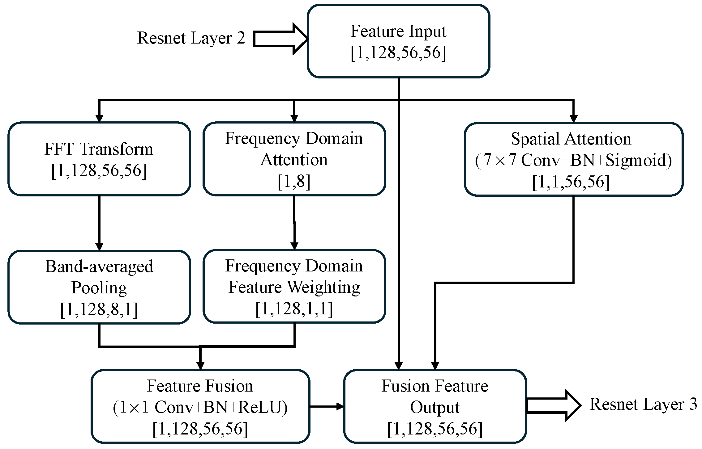
After selecting the original input features, an enhanced frequency-domain attention mechanism is introduced based on the original network in ResNet18. Specifically, feature maps output by ResNet Layer 2 are fed into the Enhanced Frequency-Domain Attention (EFDA) module, which adaptively enhances features in both spatial and frequency domains. The connection diagram of the EFDA module is presented in Figure 2, where numbers in square brackets denote the data dimensions processed by each layer.
This module comprises two parallel sub-modules: a spatial attention mechanism [30] and a frequency-domain attention mechanism. These sub-modules enhance feature maps to highlight features critical for hydroacoustic signal classification. The spatial attention branch captures salient feature regions within the time-frequency space. The frequency-domain attention branch first applies a frequency-domain transform to feature maps. It uses 2D Fast Fourier Transform (2D FFT). This maps all the channel feature maps to the frequency domain. Then, it computes magnitude spectra. These spectra characterize energy distributions across different frequency components. From an image-processing perspective, this operation decomposes spatial signals. It breaks them into components of varying frequencies. For Mel spectrograms, FFT reveals the “rate of change”. This refers to the spatial structure of Mel images. Low-frequency components correspond to slow, smooth regions. Examples include large-scale energy distributions. High-frequency components correspond to rapidly changing detail-rich regions. Examples include mutations, edges, and textures. This converts the original energy distribution in image space. It turns it into energy distributions across different variation scales. This enables the network to directly focus on useful image changes. These changes are most helpful for recognition. The network does not merely focus on specific locations in image space. Frequency-domain operations can make up for the limitations of spatial attention. Spatial attention only focuses on which part of the image is important. It cannot identify which change patterns in the image matter. For some hydroacoustic signals, the discriminative features of their Mel spectrograms do not depend solely on spatial location features in the image. The frequency structure of the energy distribution also matters. Examples include periodicity, texture, and oscillation. Focusing on both distribution and variations aligns with the scientific intuition behind traditional Mel-spectrum-processing methods.
Next, band pooling and attention allocation are performed. The spectrum is evenly divided into eight bands along the frequency axis. For each band, the energy average is calculated. This gives a compact band energy representation. Then, a lightweight Multi-Layer Perceptron (MLP) and softmax [31] activation are used. They generate attention weights for each frequency band. These weights are applied for attention-weighted feature fusion. A 1 × 1 convolution maps the weighted features back to the spatial domain. Finally, the outputs of the frequency-domain and spatial attention branches are fused. They are fused with the original features via residual concatenation. This produces the enhanced feature representation. Notably, in feature fusion, the proposed method did not use methods like inverse Fourier transform. Such methods map the frequency-domain weighting back to the feature map. Instead, the proposed method employs the 1 × 1 convolution [32,33] for this mapping. This approach is similar to global modulation in channels. It amplifies channels in the feature map. These channels have high attention weights in the frequency bands of interest. In contrast, inverse FFT is more like spatial modulation. The method already has a spatial attention mechanism. So using channel-level global modulation is more comprehensive and efficient.
In summary, the EFDA module works as follows. It enables the network to focus adaptively on the most discriminative variability and spatial regions. This design aims to improve robustness. It also enhances the effectiveness of feature extraction. These improvements target hydroacoustic target classification tasks.

2.2. Classifier Design

To address the challenges of few-shot and incremental learning in underwater-acoustic target recognition and classification, this project uses a prototype-based classification framework in the classifier module. After feature extraction, the network draws on the concept of Prototypical Networks. It constructs distinct classification prototypes for each category before classification. For each category in the current training phase, the feature vectors of its support samples are averaged in the embedding space. This forms the prototype of that category. In the inference phase, the similarity between the query sample’s features and all the category prototypes is calculated. The category with the highest similarity is taken as the prediction result. To further enhance the discriminative ability of the prototypes, the model introduces a self-attention mechanism. This happens after concatenating the prototypes and query features. The mechanism adaptively models inter-category and intra-category relationships.
For each category, the feature representations of samples, which, in support set F sup , are first extracted, are denoted as
F sup ( k · n ) = x k n , k = 1 , 2 , , K ; n = 1 , 2 , , N
where x denotes the training samples, N the number of classes, and K the number of support samples within each class. The feature vectors of support samples for each class are averaged along the sample dimension (N) to obtain the prototype vector ( P n ) for each class, denoted as
P n = p 1 , p 2 , , p N = 1 N k = 1 K F sup ( k · n ) .
Query samples corresponding to each category are extracted from the training set, and their features are denoted as q. Subsequently, all the category prototypes are concatenated with the query feature to form a feature sequence as
S = p 1 , p 2 , , p N , q
which encapsulates the complete contextual information for the current few-shot task. This concatenated feature sequence is then fed into a multi-head self-attention module for enhancement. This module dynamically refines the feature representation of each element by computing the correlations between any two elements in the sequence. The computation process for a single self-attention head is as follows:
A head i = softmax Q K T d i V
where softmax [31,34] is an activation function that converts a vector of real numbers to a probability distribution. Each element involved in the calculation ranges from 0 to 1, and the sum of all the elements is 1. The use of the softmax operation here allows the output to be normalized into class probabilities. The query matrix (Q), key matrix (K), and value matrix (V) are all subspace matrices obtained by projecting the sequence (S) through distinct linear transformations, and d i is the dimension of each head. The projections for each subspace are learned independently to leverage the same input features from different perspectives. The multi-head mechanism computes all the A head values in parallel, concatenates the results, and fuses them through a linear layer as
S = Norm S + A head 1 , A head 2 , , A head N = P N , q
where “Norm” refers to layer normalization [35], which function is to normalize the feature dimensions after connection. Each element in the enhanced sequence thus incorporates information from all the other class prototypes and query samples within the task. Let p denote the enhanced prototype and q represent the enhanced query feature. Cosine similarity is computed between these two as
sim n = q · p n q p n , n = 1 , 2 , , N .
The class with the highest similarity score is taken as the prediction result, and the specific implementation process of this part is provided in the pseudocode in Table 1.
This study uses a prototype-based classifier mainly to enhance the network’s classification decisions in few-shot incremental learning scenarios. Prototypical networks work on a core idea: for each category, the mean feature of support set samples serves as the category’s prototype. Then, query samples are compared with all the prototypes by calculating similarity. The category with the highest similarity score is taken as the predicted class. The proposed method has significant advantages over standard prototypical networks. First, during training, prototypes are dynamically updated under the multi-head attention mechanism. They are not static feature means, like those in traditional approaches. Instead, they adaptively adjust based on the current task context. This allows better adaptation to category distributions across different tasks. Second, query samples integrate prototype information from all the categories. This enhances feature representations and further improves the model’s discriminative capability. Finally, the multi-head attention mechanism can implicitly model inter-category relationships (e.g., similarities and differences). This provides richer information for the classification task.
In summary, adding the multi-head self-attention mechanism to prototypical networks helps the model to effectively use intra-task contextual information. This improves classification performance in complex few-shot scenarios.

2.3. Training Strategies

Regarding the learning strategy, this method adopts a session-wise incremental learning process. The base session employs an episode-based training approach to train base categories. In each subsequent session, only a few shots of samples from new categories are introduced for incremental training.
The base session is designed to simulate the network’s pre-training process in practical application scenarios. Typically, relatively sufficient data are available for training in such scenarios. To ensure performance in subsequent few-shot incremental learning, an episode-based training paradigm is used at this stage. It simulates few-shot task scenarios. Specifically, the data extractor randomly selects N categories from the current training batch. These categories serve as input for the current training episode. For each category, K samples form the support set, and 3 K samples make up the query set. Thus, each batch corresponds to a few-shot task. The support set is used to compute each category’s prototype. The query set evaluates the model’s ability to classify new samples. Classification loss is calculated based on the query set’s predicted results and their corresponding ground-truth labels.
In the incremental learning stage, for each new category, the prototype is computed as the mean of its support samples’ feature representations. This prototype is then added to the classification head as the new category’s weight. It can also replace existing weights when needed. This phased incremental update strategy allows the model to continuously learn new categories. At the same time, it effectively mitigates catastrophic forgetting. Lastly, multiple loss functions are employed in this network, i.e.,
L total = L C E + w freq · L freq .
The hyperparameter w freq is the weight factor for frequency-domain-enhanced attention. Adjusting it allows flexible tuning of the optimization priority during training to achieve efficient collaborative optimization. The classification loss ( L C E ) adopts the cross-entropy loss function [36], which measures the discrepancy between the class probability distribution output by the model and the ground-truth labels during classification training. Its formula, according to reference [36], can be expressed as follows:
L C E = 1 N k = 1 K n = 1 N y ( k · n ) log e ( k · n )
where y is the ground-truth label of the sample, N the number of classes, K the number of support samples within each class, and e the model’s prediction accuracy for sample y. On the other hand, the enhanced frequency loss ( L freq ) consists of four components, i.e.,
L freq = α · L div + β · L cont + γ · L cons + λ · L p r
where α , β , γ , and λ are hyperparameter weights. The EFDA uses four types of loss functions, which are as follows:
(1)
L div represents the diversity loss, which is the sum of off-diagonal elements, by computing the covariance matrix of frequency-band attention weights. This loss is designed to encourage diversity in the distribution of attention weights across different frequency bands. It prevents all the frequency-band weights from converging to uniformity;
(2)
L cont is the contrast loss, and it calculates distances between categories. It encourages increasing these distances to enhance the discriminability of category features;
(3)
L cons is the consistency loss, and it computes the variance of features within the same category to encourage a reduction in variance. This process compactifies the feature distribution within each category, thereby enhancing intra-class consistency;
(4)
L pr is the frequency prior loss, and it is used to manually guide the model to focus on specific frequency bands. This process enhances sensitivity to critical frequency ranges.
Diversity loss ( L div ) can be calculated using the following formula:
L div = i = 1 B f j = 1 B f 1 B s A T A i j s . t . i j
where A is a decentralized matrix ( · i j ) taking the element in the ith row and jth column in the matrix. It is composed of attention weights from all the frequency bands. B f represents the number of prior-focused frequency bands, B s the batch size. Taking the modulus of the off-diagonal elements of the correlation matrix yields the non-negative correlation magnitude of the attention between different frequency bands. By summing these values, frequency bands with stronger correlations contribute more positive loss. The model is then urged to reduce such inter-band correlations by updating parameters to minimize this loss. This operation increases diversity in the frequency-band attention distributions across different samples. In turn, it enhances the model’s ability to represent diverse frequency-domain features and improves the model’s generalization capability. Contrast Loss ( L cont ), inspired by reference [37], can be expressed as
L cont = i j E exp f x i f x j 2
where f x denotes the output of the feature extractor for the category feature (x). E · is the mathematical expectation operation. The Euclidean distances between features of different categories are converted to similarity metrics through the inverse operation of an exponential function. Specifically, the output approaches 1 when the distance in the feature space is smaller and approaches 0 when the distance is larger. Thus, this loss can be used to measure the discriminability of category features. Consistency loss ( L cons ) can be expressed as
L cons = i j E f x ^ i f x ^ i 2 2
where · 2 2 involves taking the L2 norm, followed by squaring the result. x ^ represents the features of the same category. Frequency prior loss ( L pr ) can be expressed as
L pr = 1 B f B s i = 1 B s j = 1 B f a ( i , j )
where a ( i , j ) represents the attention weight of the jth frequency band in the ith sample. Considering the characteristics of the Mel spectrum, the proposed method adopts a prior regularization to reduce the weights of the lowest and highest frequency bands. This allows the model to focus more on stable periodic patterns with non-volatile changes, thereby reducing undesigned impacts from factors such as noise.
The parameter update process of the proposed network is divided into two sessions. During the base session, the Stochastic Gradient Descent (SGD) [38] optimizer is employed to minimize the weighted sum of the cross-entropy loss and frequency-domain loss. This session utilizes standard backpropagation with gradient descent. In the incremental session, the mean of the support set features for each new category is computed to form its prototype, which is then appended to the weights of the fully connected layer.
The loss functions designed in this study balance classification accuracy and frequency-domain discriminability. They enable efficient incremental learning through prototype replacement and fine-tuning. All the losses are optimized via standard backpropagation to ensure end-to-end trainability and good generalization. The prototypical network component does not introduce additional loss functions but, instead, drives training through classification losses. Its training objective is to minimize classification error. Meanwhile, the global attention mechanism enhances the representability of prototypes and query features by modeling inter-class and intra-class relationships. This module also does not introduce new loss functions, just acting as a feature enhancement layer which outputs contribute to the final classification loss.
Compared with traditional classification networks, the proposed method avoids extensive parameter updates required in incremental scenarios. During incremental learning, parameters associated with existing category prototypes remain unchanged, with only new prototypes added for training. This is expected to mitigate catastrophic forgetting caused by few-shot incremental learning.

3. Evaluation

Based on the ShipsEar [17] dataset, the experimental results will be presented and discussed, along with the outcomes of several ablation studies. These results demonstrate explorations into few-shot incremental learning for underwater-acoustic target recognition.

3.1. Dataset

The ShipsEar dataset consists of recordings collected by hydrophones deployed at docks, capturing various ship noises corresponding to berthing or departing maneuvers. Since the sounds were recorded in a real underwater environment at a depth of 15 m, both artificial and natural background noises are present in the signals. The dataset comprises ninety WAV-format recordings across five categories. Each category contains one or more targets, with the duration of each audio segment ranging from 15 s to 10 min.
This paper segments all the signals into fixed 5 s clips, resulting in 1956 labeled sound samples. The category labels are divided into 12 subcategories according to the dataset’s guidelines. Among these twelve subcategories, the dataset selected six with relatively more data as the base-training set, and the remaining six as the incremental training set, as shown in Table 2. Session 0 is designed to simulate the pre-training phase before the deployment of underwater detection tasks. In practical applications, this phase usually involves sufficient training on all the known category data; therefore, the dataset provides six categories of data with as many snapshots as possible for this phase. Sessions 1 to 6 correspond to the incremental phases, simulating scenarios where new category-streaming data are encountered under underwater detection conditions. Providing a small number of training samples for new categories in each incremental learning phase can effectively test the network’s few-shot incremental learning capability. The base dataset is split into training and testing sets at a 7:3 ratio. For each session in the incremental training set, K-shot samples were extracted as the training set, and the rest served as the testing set.
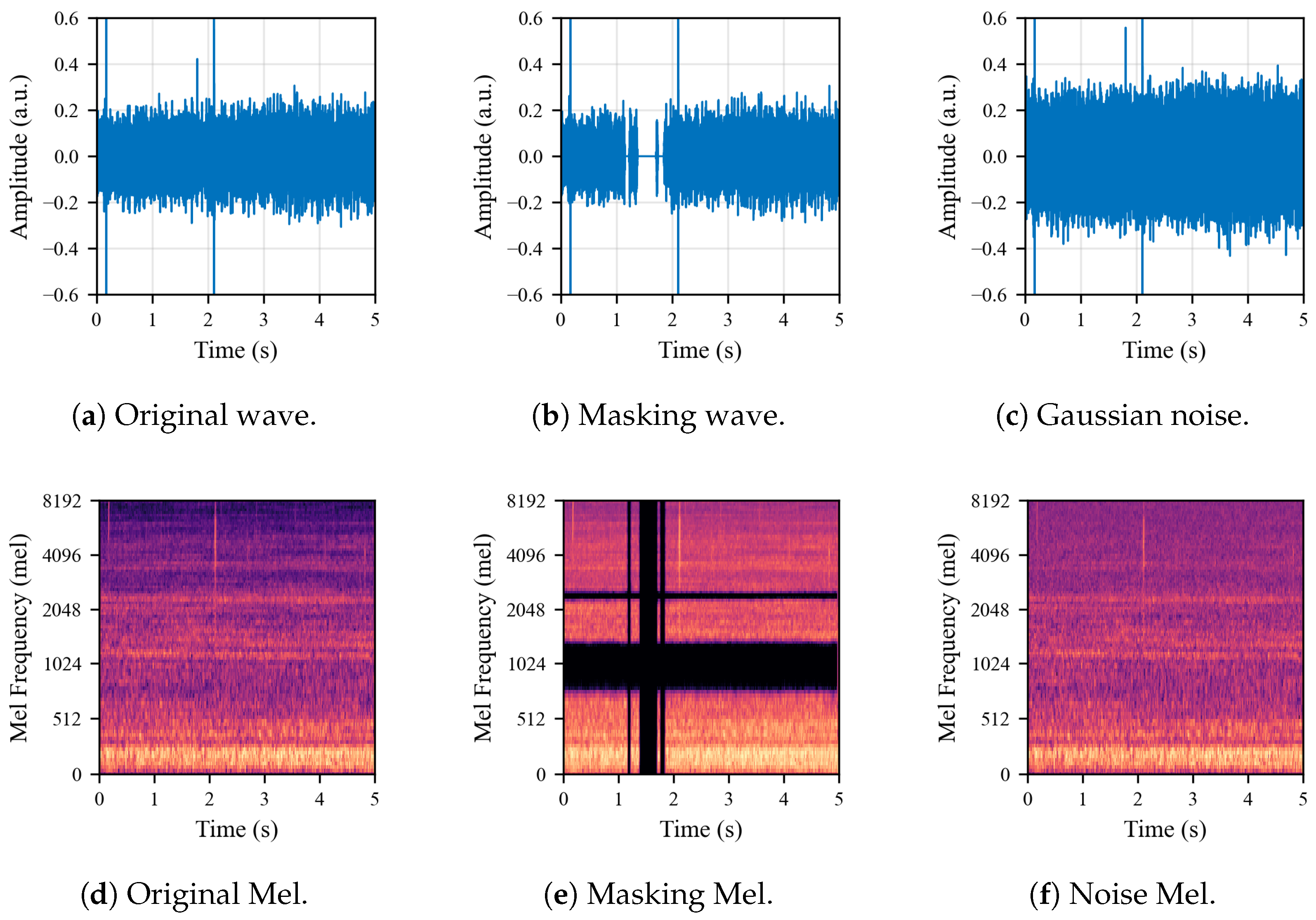
In the dataset, the method performed conventional data augmentation techniques, such as adding Gaussian noise, masking, and cropping, to expand the data volume for base training. The masking operation randomly selects from one to five segments along both time and frequency dimensions of each original signal sample, setting their values to zero to simulate missing data and enhance model robustness to incomplete or corrupted inputs. Examples of pre-processing operations are illustrated in Figure 3. Notably, to preserve the physical meaning of Mel spectrograms (i.e., the distribution of energy in the time-frequency domain) the method proposed did not adopt the random rotation augmentation method commonly used in most vision recognition approaches.

3.2. Results

First, this paper constructed six incremental learning sessions, each containing one category from the incremental training set with random order. For each category in the incremental training set, five-shot samples were extracted to form these six few-shot incremental sessions. All the methods involved in the comparative experiments were subjected to a maximum of 100 base-training epochs under the same dataset partitioning, with each few-shot incremental session undergoing a maximum of 50 training epochs.
The proposed method employs the SGD optimizer with a momentum of 0.9. Both the base-learning rate and incremental learning rate are set at 0.001, with a weight decay of 0.0001. The milestone-based learning rate scheduling was adopted. The milestones were set at 40% and 70% of the total training epochs, and the learning rate was multiplied by 0.1 at each milestone. The batch size was set at 32 in the base-training phase. Each training episode in the base training includes five categories with five support samples and fifteen query samples per category. Each training epoch consists of 50 episodes. In incremental learning, only the few-shot training dataset with five samples is used for incremental training per new category. This simulates the harsh stream-processing scenarios of underwater-acoustic target recognition in real-world applications.
For parameters related to the frequency-domain attention mechanism, the number of frequency bands is set at 8, and the initial weights for all the frequency-domain enhancement losses are set at 0.1. All the experiments are conducted in a single Graphics-Processing-Unit (GPU) environment. The comparison results with classical few-shot deep learning methods and incremental learning methods are presented in Table 3. The baseline here refers to the basic ResNet18 architecture combined with a fully connected structure.
Each column in the table represents the recognition accuracy of a single session. The performance-dropping rate (PD) characterizes the magnitude of the performance degradation in few-shot incremental learning. As shown in Table 3, while TADAM and Dense-CNN achieve slightly higher base accuracies than CNN and LSTM in session 0, they still lack incremental learning capabilities. In incremental sessions 1 to 6, models may suffer from catastrophic forgetting, leading to a sharp drop in the overall recognition accuracy. These conventional networks exhibit over 60% PD, with some even approaching 80% PD, indicating catastrophic forgetting when learning new few-shot categories. In contrast, few-shot incremental methods (prototypical, IPN, iCaRL, and CEC) limit PD to below 40%, confirming their incremental capabilities. The base recognition accuracy of UACIL reaches 92.89%, and the overall accuracy remains at 68.44% after six increments. Compared with the baseline method, UACIL has a base accuracy that is improved by 11.14%, and the performance-dropping rate in incremental learning is reduced by 50.09%. The proposed method outperforms other few-shot incremental learning methods in base class recognition accuracy. Meanwhile, it effectively mitigates catastrophic forgetting during incremental learning.
Table 4 presents the average recognition accuracies of various methods for six incremental few-shot categories in the five-shot setting. It can be observed that the proposed method outperforms other presented methods. This indicates that the proposed method exhibits superior ability to reduce overfitting. However, the recognition accuracy remains unsatisfactory, and the reasons are analyzed at the end of this section. Regarding the computational efficiency of the proposed network, its total Floating-Point operations (FLOPs) are approximately 3.5 million, among which ResNet18 contributes about 3.2 million. In the GPU environment of the experimental platform in this paper, the average inference time for single-shot data is approximately 0.67 ms, which fully meets real-time requirements.
To further validate the proposed method and determine which pre-processing method for underwater-acoustic signals yields the optimal classification performance, this paper tested different pre-processings as inputs. The underwater-acoustic features investigated include raw sound waveforms, time-frequency spectrograms, MFCC spectrograms, and Mel spectrograms. With the dataset composition and partitioning unchanged, only the input-image-processing methods were replaced. The test results are presented in Table 5.
It can be observed that the enhanced frequency-domain attention mechanism of the proposed method can better extract image classification features with rich variation information. The proposed method exhibits limited capability in analyzing the features of waveforms. MFCC and STFT are essentially image features that reflect the time-frequency domain information of signals. Thus, their recognition results are much better than those of the waveform but slightly inferior to those of the Mel spectrogram. On the contrary, Mel spectrograms, which contain abundant detailed information, are more compatible with the frequency-domain attention mechanism in this study, achieving the best classification results.
Subsequently, with Mel spectrograms as input, classification in different frequency bands is performed. The results are presented in Table 6. It can be observed that the highest recognition accuracy is achieved for the eight-frequency-band configuration. The frequency-band attention mechanism shows an admirable advantage in this step, while the loss of continuous information, caused by excessively fragmented frequency-band divisions, is totally avoided.
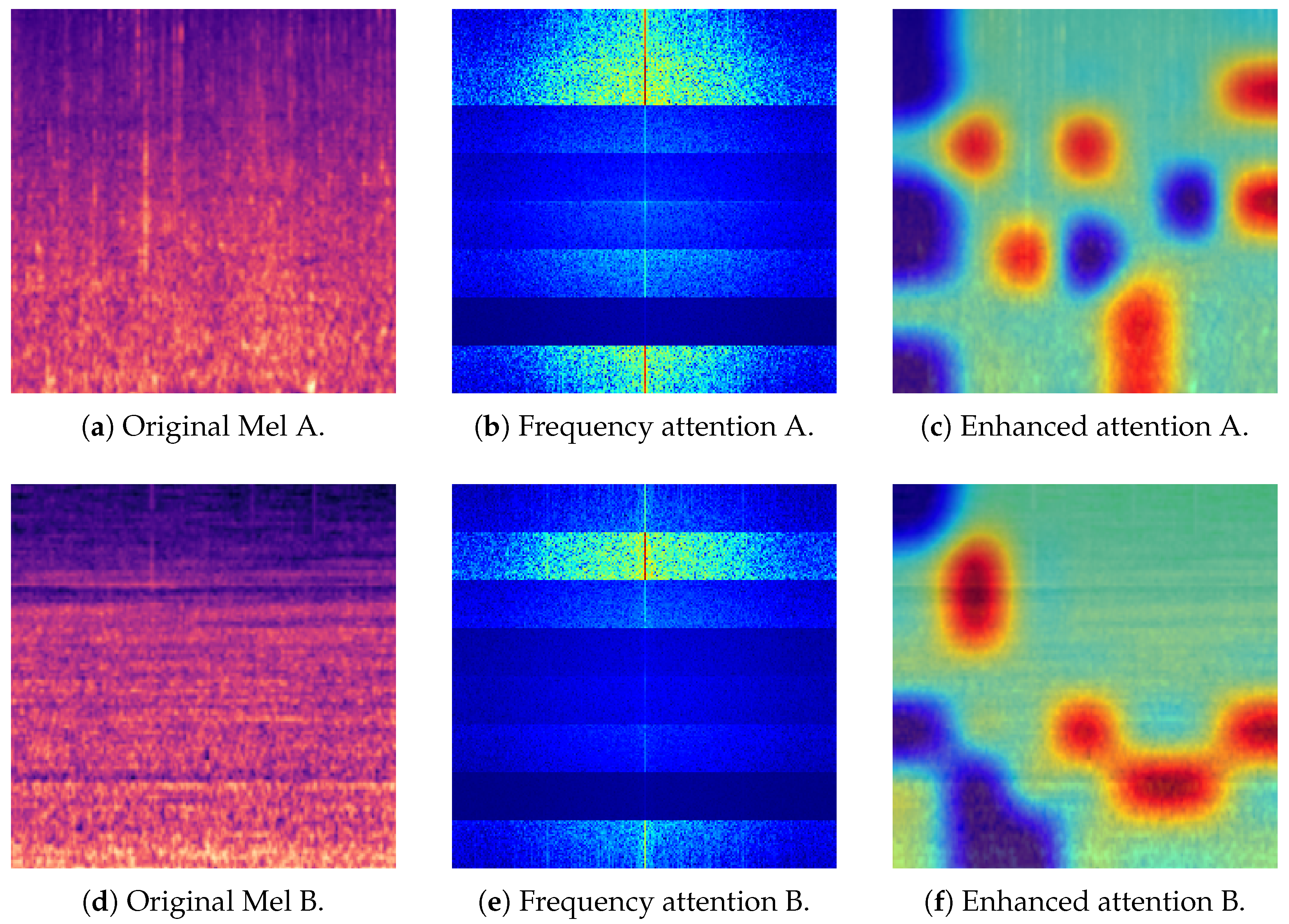
Further, to study the feature extraction component of the enhanced frequency-domain attention mechanism, Figure 4 presents the attention-mapping results of different categories, mapped back to the original images. The frequency-domain attention mechanism in this study accounts for both spatial positions and variation characteristics, enabling more comprehensive and effective extraction of classification features.
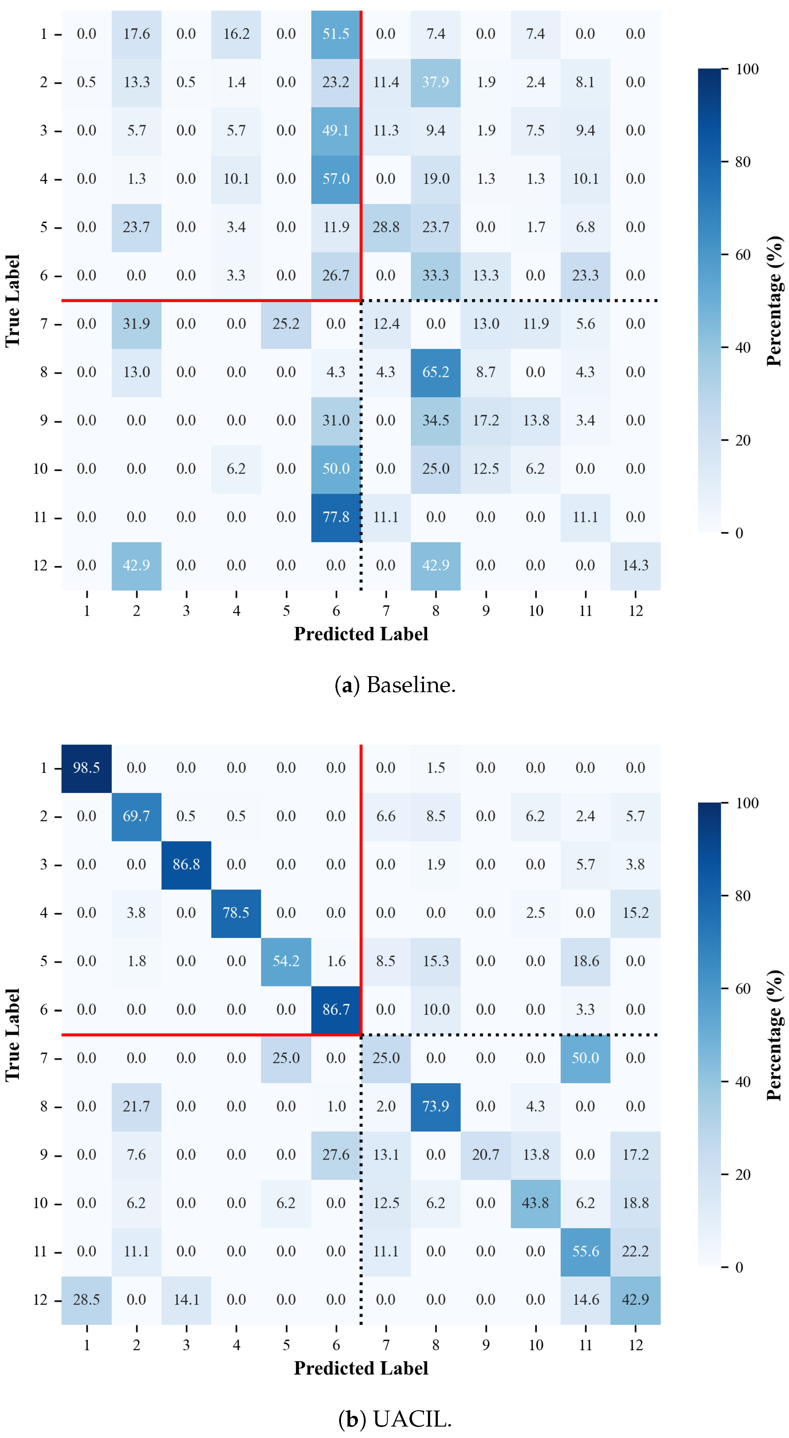
To verify the improvement in the proposed method over the baseline without an incremental learning module, Figure 5 presents the confusion matrices of both the baseline and the proposed method after incremental learning. The red-boxed area at the upper left corresponds to the base session portion. The training involved six incremental sessions, with one new category added per session; the results for these categories are enclosed in dashed boxes. The baseline network exhibited severe catastrophic forgetting during incremental learning, losing its original ability to classify the six pre-trained base categories. In contrast, the incremental learning method designed in this study effectively mitigated catastrophic forgetting. Although recognition results for some few-shot incremental categories were not entirely satisfactory, the classification ability for the original categories remained reliable.
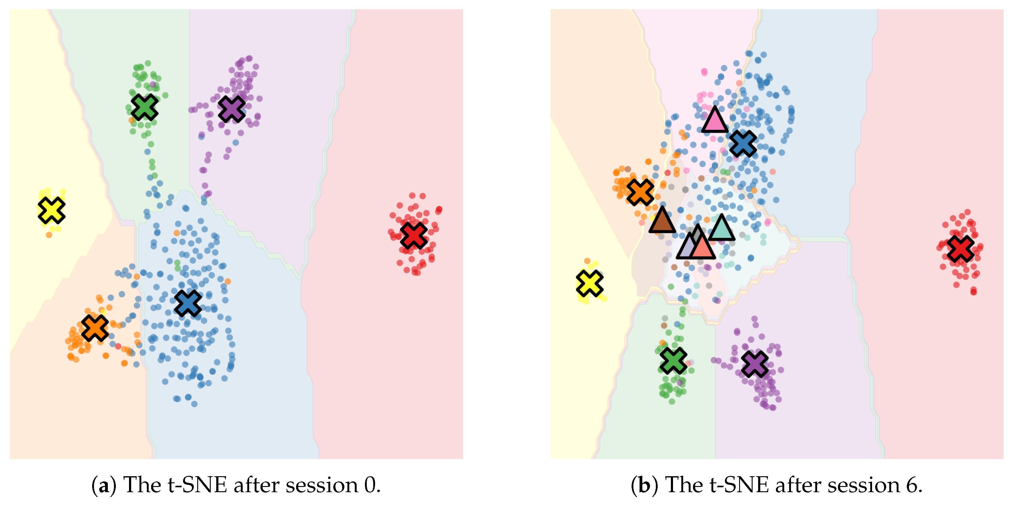
To analyze the network’s contribution to overcoming catastrophic forgetting, Figure 6 shows T-distributed Stochastic Neighbor Embedding (t-SNE) [39] dimensionality reduction plots before and after incremental learning. The t-SNE maps high-dimensional data to a low-dimensional space while preserving the similarity relationships between data points as much as possible. It first calculates the similarity between data points in the high-dimensional space and converts it to a probability distribution and then constructs a corresponding probability distribution in the low-dimensional space. Dimensionality reduction is achieved by minimizing the difference between the two probability distributions. In this paper, t-SNE is used for visualizing classification prototypes, which allows for a more intuitive observation of prototype distributions and an exploration of the network’s classification performance. In Figure 6, the points of different colors represent data points from different categories. Crosses indicate the classifier prototypes before the increment, triangles represent the classifier prototypes after the increment, and background color blocks denote classification boundaries.
The plots in Figure 6 demonstrate that the incremental learning process successfully maintains the classification capability acquired during base training, thereby avoiding catastrophic forgetting. The proposed method effectively preserves the aggregation degree of the original categories during incremental learning, overcoming the catastrophic forgetting caused by few-shot increments, because in few-shot incremental training, the number of samples involved in training is extremely small. Such a scarcity of samples leads to uncertainty in prototype estimation. When reflected in the high-dimensional space, this manifests as the feature distributions of similar categories being close to each other or even overlapping. This phenomenon is reflected in Figure 6b. The distributions of classification prototypes among incremental categories are not effectively separated, which also contributes to the suboptimal recognition performance of some new few-shot categories, as shown in Table 4.
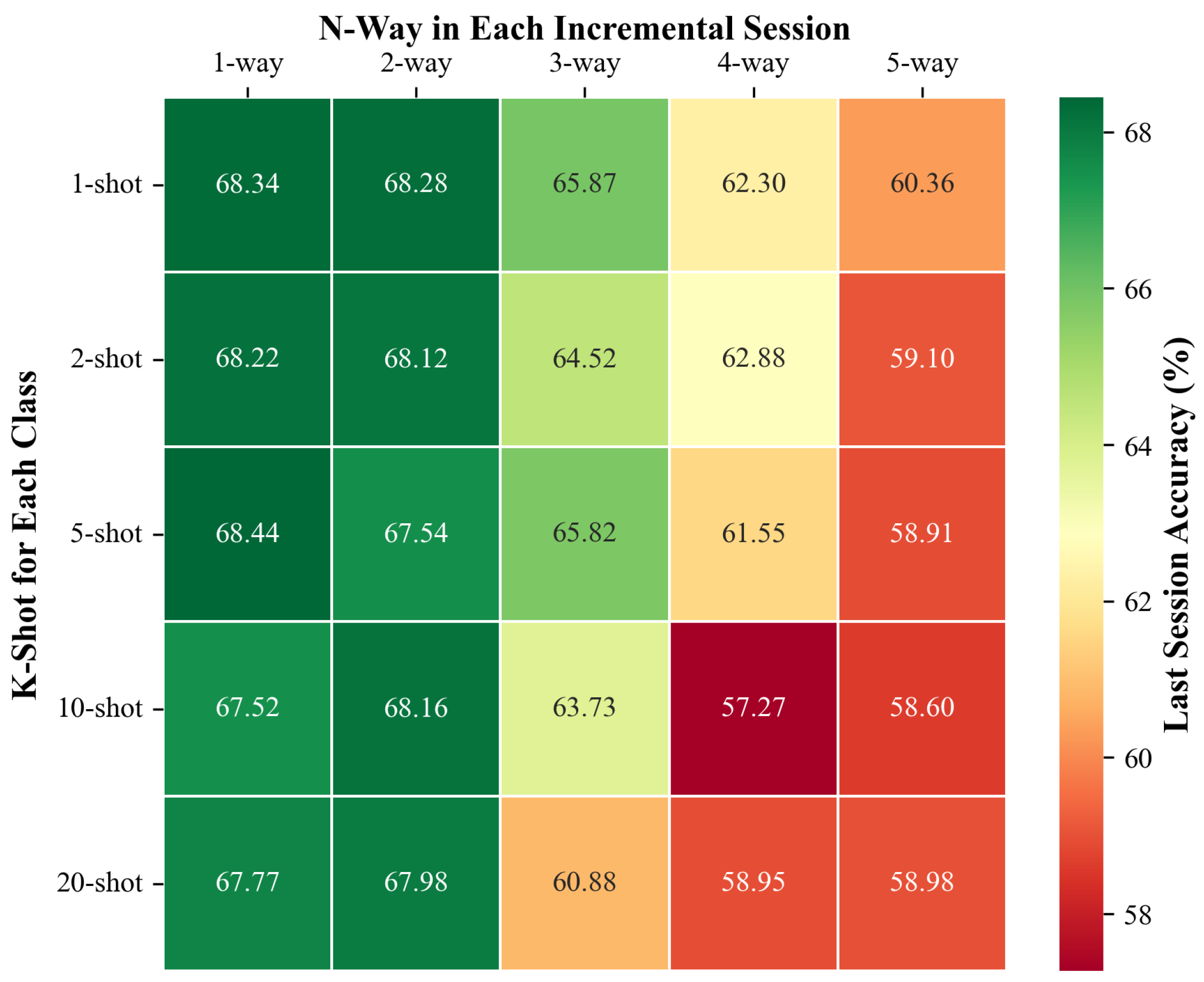
Then, this paper tested the classification capability of the proposed method in scenarios involving simultaneous training with different numbers of new categories and in different few-shot settings. Figure 7 shows the performance of the method in various N-way K-shot configurations. For different way numbers, this paper constructed sessions using as many incremental categories as possible. For example, in the case with three ways, there are two sessions in total, while each session contains three categories and K samples per category. The accuracy of the last session is taken as the final comparison. It can be observed that under few-shot conditions, the number of shots has little impact on the recognition results. However, in incremental learning, the recognition results are inversely proportional to the number of newly added categories in one session. This is because the number of categories in the base-session-training data remains relatively small, and the generalization is, thus, insufficient when performing simultaneous incremental learning with multiple few-shot categories, which, in turn, causes a decline in network performance. Based on the above results, this paper recommend adding only one category at a time during the incremental session when the data categories for base training cannot be directly expanded. This not only aligns well with streaming data-processing scenarios but also enables the network to maintain relatively excellent recognition performance.

4. Conclusions

This paper focuses on the problem of recognizing few-shot categories in streaming data scenarios for underwater-acoustic target recognition and proposes a network model named UACIL for few-shot class-incremental training in such streaming data-processing scenarios. The model can adaptively expand its classification capacity while retaining existing knowledge when training in new few-shot classes. During the base-training session, the proposed approach uses a prototype classifier to simulate few-shot learning via episodic learning. In the incremental training session, only a part of the feature extraction network and the extended classification head are trained to reduce catastrophic forgetting. Within the feature extraction network, this paper introduces an enhanced frequency-domain attention mechanism that focuses on both spatial features and variations of Mel spectrograms. Additionally, a composite loss function is designed for the network, which significantly improves recognition accuracy. In the incremental experiment on the ShipsEar dataset, the base recognition accuracy of UACIL reaches 92.89%, and the overall accuracy remains at 68.44% after six increments. Compared with the baseline method, the base accuracy is improved by 11.14%, and the performance-dropping rate in incremental learning is reduced by 50.09%. The proposed method outperforms other comparative methods. Furthermore, this paper quantitatively analyzed the impact of each module in the proposed method and visually evaluated the effect of this method on alleviating catastrophic forgetting in Section 3.2. The experimental results validate the feasibility of this approach, confirming its effectiveness in mitigating catastrophic forgetting.
However, the model’s few-shot recognition performance still has room for improvement. Specifically, the prototype distances of new categories are insufficient, resulting in suboptimal classification performance for some new classes. Accordingly, this will be the focus of our team’s next research phase. We will further explore model optimization strategies to increase prototype distances, thereby enhancing the few-shot classification capability.

Author Contributions

Conceptualization, W.W. and D.Z.; methodology, W.W.; software, W.W.; validation, Y.L.; formal analysis, D.Z.; investigation, T.S.; resources, D.Z.; data curation, Y.L.; writing—original draft preparation, W.W.; visualization, W.W.; supervision, D.Z.; project administration, T.S. and Y.L.; funding acquisition, D.Z. All authors have read and agreed to the published version of the manuscript.

Funding

This research received no external funding.

Institutional Review Board Statement

Not applicable.

Informed Consent Statement

Not applicable.

Data Availability Statement

Data are available in a publicly accessible repository. The data used in this study are openly available at https://underwaternoise.atlanttic.uvigo.es/ (accessed on 25 July 2025).

Conflicts of Interest

The authors declare no conflicts of interest.

References

  1. Luo, X.; Chen, L.; Zhou, H.; Cao, H. A Survey of Underwater Acoustic Target Recognition Methods Based on Machine Learning. J. Mar. Sci. Eng. 2023, 11, 384. [Google Scholar] [CrossRef]
  2. Liu, F.; Shen, T.; Luo, Z.; Zhao, D.; Guo, S. Underwater target recognition using convolutional recurrent neural networks with 3-D Mel-spectrogram and data augmentation. Appl. Acoust. 2021, 178, 107989. [Google Scholar] [CrossRef]
  3. Tang, J.; Ma, E.; Qu, Y.; Gao, W.; Zhang, Y.; Gan, L. UAPT: An underwater acoustic target recognition method based on pre-trained Transformer. Multimed. Syst. 2025, 31, 50. [Google Scholar] [CrossRef]
  4. Cui, X.; He, Z.; Xue, Y.; Tang, K.; Zhu, P.; Han, J. Cross-Domain Contrastive Learning-Based Few-Shot Underwater Acoustic Target Recognition. J. Mar. Sci. Eng. 2024, 12, 264. [Google Scholar] [CrossRef]
  5. Shi, B.; Sun, M.; Puvvada, K.C.; Kao, C.C.; Matsoukas, S.; Wang, C. Few-Shot Acoustic Event Detection Via Meta Learning. In Proceedings of the ICASSP 2020—2020 IEEE International Conference on Acoustics, Speech and Signal Processing (ICASSP), Barcelona, Spain, 4–8 May 2020; pp. 76–80. [Google Scholar] [CrossRef]
  6. Wu, Y.; Li, Y.; Zhao, T.; Zhang, L.; Wei, B.; Liu, J.; Zheng, Q. Improved prototypical network for active few-shot learning. Pattern Recognit. Lett. 2023, 172, 188–194. [Google Scholar] [CrossRef]
  7. Cheng, H.; Wang, Y.; Li, H.; Kot, A.C.; Wen, B. Disentangled Feature Representation for Few-Shot Image Classification. IEEE Trans. Neural Netw. Learn. Syst. 2024, 35, 10422–10435. [Google Scholar] [CrossRef] [PubMed]
  8. Wen, W.; Liu, Y.; Lin, Q.; Ouyang, C. Few-shot Named Entity Recognition with Joint Token and Sentence Awareness. Data Intell. 2023, 5, 767–785. [Google Scholar] [CrossRef]
  9. Duan, R.; Li, D.; Tong, Q.; Yang, T.; Liu, X.; Liu, X. A Survey of Few-Shot Learning: An Effective Method for Intrusion Detection. Secur. Commun. Netw. 2021, 2021, 4259629. [Google Scholar] [CrossRef]
  10. Zeng, W.; Xiao, Z.-Y. Few-shot learning based on deep learning: A survey. Math. Biosci. Eng. 2024, 21, 679–711. [Google Scholar] [CrossRef]
  11. Cui, X.; He, Z.; Xue, Y.; Zhu, P.; Han, J.; Li, X. Few-Shot Underwater Acoustic Target Recognition Using Domain Adaptation and Knowledge Distillation. IEEE J. Ocean. Eng. 2025, 50, 637–653. [Google Scholar] [CrossRef]
  12. Fu, B.; Nie, J.; Wei, W.; Zhang, L. Constructing a Multi-Modal Based Underwater Acoustic Target Recognition Method with a Pre-Trained Language-Audio Model. IEEE Trans. Geosci. Remote Sens. 2025, 63, 1–14. [Google Scholar] [CrossRef]
  13. Tian, S.; Bai, D.; Zhou, J.; Fu, Y.; Chen, D. Few-shot learning for joint model in underwater acoustic target recognition. Sci. Rep. 2023, 13, 17502. [Google Scholar] [CrossRef]
  14. Yin, Q.; Shen, L. Underwater acoustic target recognition based on population balance-encoding classification. Ocean Eng. 2025, 337, 121899. [Google Scholar] [CrossRef]
  15. Bao, W.; Ren, Q.; Wang, W.; Huang, M.; Xiao, Z. A dual-label-reversed ensemble transfer learning strategy for underwater target detection. Appl. Acoust. 2025, 235, 110701. [Google Scholar] [CrossRef]
  16. Zhou, D.W.; Wang, Q.W.; Qi, Z.H.; Ye, H.J.; Zhan, D.C.; Liu, Z. Class-Incremental Learning: A Survey. IEEE Trans. Pattern Anal. Mach. Intell. 2024, 46, 9851–9873. [Google Scholar] [CrossRef]
  17. Santos-Dominguez, D.; Torres-Guijarro, S.; Cardenal-Lopez, A.; Pena-Gimenez, A. ShipsEar: An underwater vessel noise database. Appl. Acoust. 2016, 113, 64–69. [Google Scholar] [CrossRef]
  18. Oreshkin, B.; Rodríguez López, P.; Lacoste, A. TADAM: Task dependent adaptive metric for improved few-shot learning. In Proceedings of the Advances in Neural Information Processing Systems; Bengio, S., Wallach, H., Larochelle, H., Grauman, K., Cesa-Bianchi, N., Garnett, R., Eds.; Curran Associates, Inc.: Nice, France, 2018; Volume 31. [Google Scholar]
  19. Doan, V.S.; Huynh-The, T.; Kim, D.S. Underwater Acoustic Target Classification Based on Dense Convolutional Neural Network. IEEE Geosci. Remote Sens. Lett. 2022, 19, 1–5. [Google Scholar] [CrossRef]
  20. Snell, J.; Swersky, K.; Zemel, R. Prototypical Networks for Few-shot Learning. In Proceedings of the Advances in Neural Information Processing Systems; Guyon, I., Luxburg, U.V., Bengio, S., Wallach, H., Fergus, R., Vishwanathan, S., Garnett, R., Eds.; Curran Associates, Inc.: Nice, France, 2017; Volume 30, pp. 4080–4090. [Google Scholar]
  21. Ji, Z.; Chai, X.; Yu, Y.; Pang, Y.; Zhang, Z. Improved prototypical networks for few-Shot learning. Pattern Recognit. Lett. 2020, 140, 81–87. [Google Scholar] [CrossRef]
  22. Rebuffi, S.A.; Kolesnikov, A.; Sperl, G.; Lampert, C.H. iCaRL: Incremental Classifier and Representation Learning. In Proceedings of the IEEE Conference on Computer Vision and Pattern Recognition (CVPR), Honolulu, HI, USA, 21–26 July 2017; pp. 2001–2010. [Google Scholar]
  23. Zhang, C.; Song, N.; Lin, G.; Zheng, Y.; Pan, P.; Xu, Y. Few-Shot Incremental Learning with Continually Evolved Classifiers. In Proceedings of the IEEE/CVF Conference on Computer Vision and Pattern Recognition (CVPR), Nashville, TN, USA, 20–25 June 2021; pp. 12455–12464. [Google Scholar]
  24. He, K.; Zhang, X.; Ren, S.; Sun, J. Deep Residual Learning for Image Recognition. In Proceedings of the 2016 IEEE Conference on Computer Vision and Pattern Recognition (CVPR), Las Vegas, NV, USA, 27–30 June 2016; pp. 770–778. [Google Scholar] [CrossRef]
  25. Meng, X.; Liu, X.; Xu, Y.; Wu, Y.; Li, H.; Kim, K.W.; Liu, S.; Xu, Y. A Multi-Time-Frequency Feature Fusion Approach for Marine Mammal Sound Recognition. J. Mar. Sci. Eng. 2025, 13, 1101. [Google Scholar] [CrossRef]
  26. Xu, J.; Li, X.; Zhang, D.; Chen, Y.; Peng, Y.; Liu, W. Enhanced underwater acoustic target recognition using parallel dual-branch network with attention mechanism. Eng. Appl. Artif. Intell. 2025, 158, 111603. [Google Scholar] [CrossRef]
  27. Li, G.; Wu, M.; Yang, H. A new underwater acoustic signal recognition method: Fusion of cepstral feature and multi-path parallel joint neural network. Appl. Acoust. 2025, 239, 110809. [Google Scholar] [CrossRef]
  28. Hu, G.; Wang, K.; Peng, Y.; Qiu, M.; Shi, J.; Liu, L. Deep Learning Methods for Underwater Target Feature Extraction and Recognition. Comput. Intell. Neurosci. 2018, 2018, 1214301. [Google Scholar] [CrossRef]
  29. Yang, S.; Jin, A.; Zeng, X.; Wang, H.; Hong, X.; Lei, M. Underwater acoustic target recognition based on sub-band concatenated Mel spectrogram and multidomain attention mechanism. Eng. Appl. Artif. Intell. 2024, 133, 107983. [Google Scholar] [CrossRef]
  30. Jaderberg, M.; Simonyan, K.; Zisserman, A.; Kavukcuoglu, K. Spatial transformer networks. Adv. Neural Inf. Process. Syst. 2015, 28, 2017–2025. [Google Scholar]
  31. Grave, E.; Joulin, A.; Cissé, M.; Facebook AI Research, D.G.; Jégou, H. Efficient softmax approximation for GPUs. In Proceedings of the 34th International Conference on Machine Learning—Volume 70. JMLR.org, Sydney, Australia, 6–11 August 2017; ICML’17. pp. 1302–1310. [Google Scholar]
  32. Hu, J.; Shen, L.; Sun, G. Squeeze-and-Excitation Networks. In Proceedings of the 2018 IEEE/CVF Conference on Computer Vision and Pattern Recognition, Salt Lake City, UT, USA, 8–23 June 2018; pp. 7132–7141. [Google Scholar] [CrossRef]
  33. Qin, Z.; Zhang, P.; Wu, F.; Li, X. FcaNet: Frequency Channel Attention Networks. In Proceedings of the IEEE/CVF International Conference on Computer Vision (ICCV), Montreal, QC, Canada, 10–17 October 2021; pp. 783–792. [Google Scholar]
  34. Bridle, J.S. Training Stochastic Model Recognition Algorithms as Networks can Lead to Maximum Mutual Information Estimation of Parameters. In Proceedings of the Advances in Neural Information Processing Systems 2, NIPS Conference, Denver, CO, USA, 27–30 November 1989. [Google Scholar]
  35. Ba, J.; Kiros, J.R.; Hinton, G.E. Layer Normalization. arXiv 2016, arXiv:1607.06450. [Google Scholar] [CrossRef]
  36. Krizhevsky, A.; Sutskever, I.; Hinton, G.E. ImageNet classification with deep convolutional neural networks. Commun. ACM 2017, 60, 84–90. [Google Scholar] [CrossRef]
  37. Chen, T.; Kornblith, S.; Norouzi, M.; Hinton, G. A Simple Framework for Contrastive Learning of Visual Representations. In Proceedings of the 37th International Conference on Machine Learning, Virtual, 13–18 July 2020; Daumé, H.D., III, Singh, A., Eds.; PMLR; 2020; Volume 119—Proceedings of Machine Learning Research. pp. 1597–1607. [Google Scholar]
  38. Gess, B.; Kassing, S.; Konarovskyi, V. Stochastic Modified Flows, Mean-Field Limits and Dynamics of Stochastic Gradient Descent. J. Mach. Learn. Res. 2024, 25, 1518–1544. [Google Scholar]
  39. Jung, S.; Dagobert, T.; Morel, J.M.; Facciolo, G. A Review of t-SNE. Image Process. Line 2024, 14, 250–270. [Google Scholar] [CrossRef]
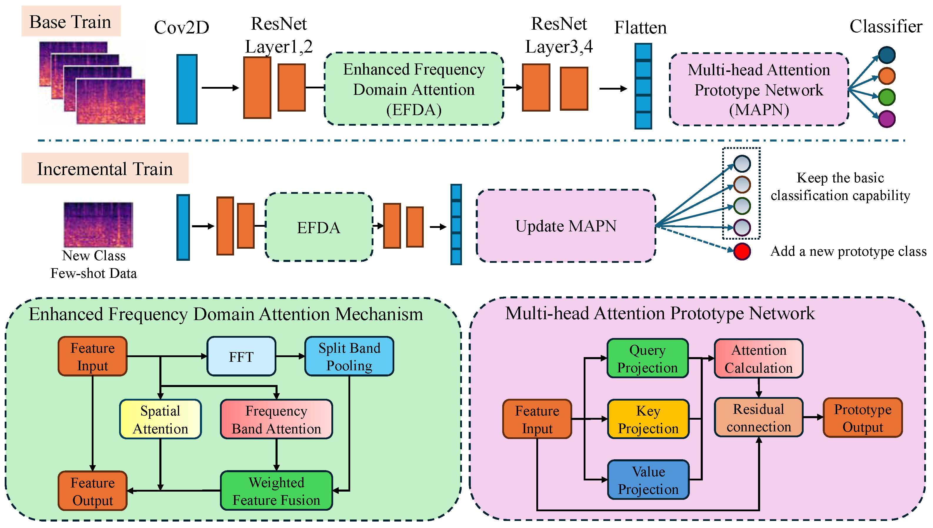
Figure 1. The overall flowchart of the system for the methodology of this paper.
Jmse 13 01606 g001
Figure 2. The workflow diagram of the enhanced frequency-domain attention module. The numbers in square brackets in the figure indicate the data dimensions processed by this layer.
Jmse 13 01606 g002
Figure 3. Examples of pre-processing operations.
Jmse 13 01606 g003
Figure 4. Visualization heatmaps of the enhanced frequency-domain attention mechanism, where spatial attention is enhanced and supplemented by the frequency-domain attention, focusing on the variation patterns of images.
Jmse 13 01606 g004
Figure 5. Comparison of confusion matrices between the baseline and the proposed method in the final session. The area circled in red indicates the base categories trained in Session 0. The results for incremental categories are enclosed in dashed boxes. Elements on the main diagonal represent the probabilities of correct estimations. Any numbers appearing outside the main diagonal of the confusion matrix mean incorrect estimations.
Jmse 13 01606 g005
Figure 6. The t-SNE [39] visualizes the data embeddings and classifier prototypes before and after incremental learning. Colors represent different categories, and the background layer indicates classification boundaries. Crosses denote prototypes of old categories, while triangles represent prototypes of new categories.
Jmse 13 01606 g006
Figure 7. Comparison of the final accuracies of models with different numbers of incremental categories and shot numbers.
Jmse 13 01606 g007
Table 1. Pseudocode for a prototype classifier network inference.
StepDescription
1Input: Support set features F sup ( k · n ) for each class, query feature Q
2Compute prototype by Equation (2) for each class
3Concatenate all the prototypes and query feature into sequence S by Equation (3)
4Apply self-attention S by Equation (5)
5Extract enhanced prototypes and enhanced query from S
6Compute similarity for each class by Equation (6)
7Apply softmax to similarities sim n to obtain class probabilities
8Output: Predicted class
Table 2. The incremental dataset consists of session 0 as the base dataset and sessions 1–6 as the incremental dataset.
SessionSession 0Session 1Session 2Session 3Session 4Session 5Session 6
ClassNatural noiseMussel boatSail boatTugboatFish boatDredgerPilot ship
Passengers
Ocean liner
RORO
Motor boat
Trawler
Samples1656957623285226
Table 3. Incremental recognition results of different networks in the ShipsEar dataset (%).
MethodSession 0Session 1Session 2Session 3Session 4Session 5Session 6PD
Baseline81.759.779.699.509.156.176.2174.54
CNN [2]80.9910.089.779.659.588.217.0473.95
LSTM [2]72.2913.2010.229.318.548.027.5564.74
TADAM [18]88.0012.2911.3010.8910.259.188.7379.27
Dense-CNN [19]84.559.479.699.499.156.216.1678.39
Prototypical [20]75.0044.2942.5041.1140.0039.0938.3336.67
IPN [21]72.9356.7255.7855.4154.2252.1946.9026.03
iCaRL [22]69.0951.5249.9647.2446.1042.1640.6628.43
CEC [23]84.8571.0369.2866.4463.7560.2858.8126.04
UACIL92.8975.4670.3169.0668.9468.5968.4424.45
Table 4. The average recognition accuracies of various methods for six incremental few-shot categories (%).
MethodBaselineCNNLSTMTADAMDense-CNNPrototypicalIPNiCaRLCECUACIL
Accuracy23.7019.1410.2630.5521.8539.0843.2141.6645.2947.65
Table 5. Incremental classification results for different hydroacoustic features using the method in this paper (%).
FeatureSession 0Session 1Session 2Session 3Session 4Session 5Session 6
Waveform47.5630.7727.3927.3427.3427.3427.34
STFT87.7072.3170.1665.1564.6864.5564.53
MFCC89.6070.6668.4368.1368.0267.9567.95
Mel92.8975.4670.3169.0668.9468.5968.44
Table 6. Incremental classification results for different frequency bands using the method in this paper (%).
BandsSession 0Session 1Session 2Session 3Session 4Session 5Session 6
187.6070.7765.8964.3463.5263.2462.95
290.4674.6568.4668.3765.9565.8065.66
491.8574.2869.8168.3167.9567.8167.48
892.8975.4670.3169.0668.9468.5968.44
1689.3574.2369.8566.5764.5264.1063.84
Disclaimer/Publisher’s Note: The statements, opinions and data contained in all publications are solely those of the individual author(s) and contributor(s) and not of MDPI and/or the editor(s). MDPI and/or the editor(s) disclaim responsibility for any injury to people or property resulting from any ideas, methods, instructions or products referred to in the content.