A Transfer Matrix Method to Dynamic Calculation and Optimal Design of Flanged Pipelines

Abstract

To study the dynamic characteristics of the fluid-filled ship piping system with flanges and to optimize the design, and based on the transfer matrix methods (TMMs), this paper proposes two modeling methods for flat-welded flanges and weld-neck flanges. Method 1 employs a lumped mass equivalent flange. Method 2, based on the finite element and analogy ideas, equates the flange to pipe sections with a larger wall thickness. By comparing with the finite element method (FEM) results, it is found that for both flat-weld flanges and weld-neck flanges, the accuracy of Method 2 proposed in this paper is superior to that of Method 1. Meanwhile, experimental verification is carried out, and the experimental results are generally consistent with those obtained using Method 2. Furthermore, the multi-objective particle swarm optimization (MOPSO) algorithm is further introduced for the dynamic design of a branch pipeline system. The goal is to avoid resonance by adjusting the natural frequency of the system. Through the comparison of the FEM results, it has been confirmed that this optimization method is both efficient and accurate in optimizing the natural frequency. The method proposed in this paper has a specific reference value for engineering practice.

1. Introduction

Pipeline vibration not only causes structural fatigue failure, leading to serious accidents, such as pipeline leakage and rupture, but also generates noise pollution, affecting the working environment and personnel health [1]. Components in the ship piping system, such as flanges and supports, can significantly alter a system’s vibration characteristics [2]. For example, as important components for supporting the pipeline, the structure and position of the support can alter the stiffness of the pipeline, thereby affecting the natural frequency of the pipeline system [3]. Therefore, a calculation method that is both accurate and efficient is particularly important for the low-vibration design of pipeline systems.

At present, the mainstream methods for calculating the fluid–structure coupling vibration characteristics of the fluid-filled pipeline include the method of characteristics (MOC), the finite element method (FEM), and the transfer matrix method (TMM). Since the fluid-conveying pipeline system exhibits a typical chain-like topology, the transfer matrix method is well-suited for such structures. The key advantage of this method is that the dimensions of the overall property matrices for the whole system do not increase with the number of elements or the system’s scale and complexity [4,5]. It offers high computational efficiency and has been widely adopted by researchers for frequency-domain fluid–structure interaction analysis in pipeline systems [6,7].

Common pipeline systems include pipeline components with regular geometric structures, such as straight pipes, elbow pipes, and branch pipes, as well as pipeline components with irregular geometric structures, such as flanges and flexible supports. Regular geometric structures pipeline components, such as straight pipes, elbow pipes, and branch pipes, can have their mathematical models established through theoretical derivation [8,9,10,11,12]. Tentarelli [8] expounded the dynamic equation of a single fluid-filled pipeline based on the transfer matrix method; Lesmez et al. [9] adopted the transfer matrix method and established the fluid–structure coupling model of the L-shaped liquid-filled pipe by equivalent the elbow pipe to multiple straight pipes; Cao et al. [10] established the mixed energy transfer matrix method (HETMM), effectively solving the problem of numerical instability existing in the vibration solution method based on TMM during high-frequency calculation, and analyzed the natural frequency of the dual-branch pipeline system; Deng et al. [11] considered the fluid friction and the flexibility correction of the elbow, calculated the natural frequency and frequency response of the Z-shaped hydraulic pipeline using TMM, and compared them with the experimental results.

The research objects in the abovementioned literature are almost all single infusion tubes or branch pipes, while in real life complex pipeline systems often connect individual pipeline components through flanges. The two commonly used types of flanges are flat-weld flanges and weld-neck flanges. In the existing literature, there is no recognized transfer matrix model for pipeline flanges, which restricts the application of the transfer matrix method in the analysis of multi-component series pipeline systems. Li [6] treated the flat-weld flange as a lumped mass and established its point transfer matrix through the balanced relationship of the force and torque before and after the flange. Liu et al. [12] considered the lateral vibration of the pipeline, established a transfer matrix model of lumped mass, and introduced a coupling term to describe the influence of eccentric mass on bending moment and shear force. The above analyses simplify the flange to a lumped mass and have not been verified through a real pipeline system. Flat-weld flanges are generally of an axisymmetric structure, and their center of mass is usually located on the axis. However, weld-neck flanges are relatively longer than flat-weld flanges, and their mass distribution is uneven. Therefore, they cannot be simply regarded as lumped mass. To address these limitations, this paper develops two transfer matrix modeling methods for flat-weld and weld-neck flanges, respectively. By introducing concepts from finite element discretization and geometrical analogy, we can improve the accuracy of dynamic characteristic analysis for flange-containing pipeline systems.

Adjusting the parameters of the pipeline system can significantly improve its vibration characteristics [13]. However, pipeline systems often contain complex components, such as flanges and flexible supports. Therefore, it is of great practical significance to establish a method for the optimal design of pipeline systems that can consider complex pipeline components. Kwong et al. [14] optimized the support position using the genetic algorithm and verified the optimization effect of the vibration and noise of the pipeline system through experiments; Wan et al. [15] conducted static and modal analyses on the pipeline system and selected the methods for pipeline support based on the risk level to accurately identify the supports with abnormal conditions and achieve the assessment of the support status of the pipeline system. Zhang et al. [16] studied the frequency adjustment and dynamic response reduction in the multi-support pipeline system through experiments and numerical simulations and introduced the multi-objective genetic algorithm to optimize the support position and adjust the first-order natural frequency to avoid the operating range of the engine. The abovementioned studies all conducted regular analyses based on the assumption that the support base is rigid but did not comprehensively consider the influence of the flexibility of the support base on the inherent characteristics of the pipeline system, which has certain limitations.

This paper initially presents the derivation and validation process of the transfer matrix model for pipe flanges, drawing on the concepts of finite element discretization and analogy. It then introduces the multi-objective particle swarm optimization (MOPSO) algorithm, aiming to optimize the pipeline design by avoiding excitation frequencies. This approach provides a reliable theoretical foundation and technical support for the engineering practice of pipeline systems.

2. Mathematical Models

2.1. Dynamic Models of Typical Pipe Components

The local coordinate system of the straight pipe is established according to the right-hand rule: along the axial direction of the pipe is the z direction, and the y-z plane is the horizontal plane. The force diagram of the fluid-filled straight pipe is shown in Figure 1. To simplify the calculation, the influence of gravity is ignored. Each straight pipe microelement includes six forces, six velocities, sound pressure, and fluid vibration velocity, totaling 14 variables. According to their vibration forms, they can be classified into three types, namely axial vibration, lateral vibration, and torsional vibration. Like straight pipes, the fluid–structure coupling mathematical models of elbow pipes can also be divided into the axial 4-equation, the y-z plane 4-equation, the x-z plane 4-equation, and the torsion 2-equation.

The 14-equation model in reference [17] is used for research. Whether it is a straight pipe or an elbow pipe element, the 14-equation model of fluid–structure coupling can be written in the following general form:

$${\mathbf{A}}_I{\displaystyle \frac{\partial y(z,t)}{\partial t}}+B{\displaystyle \frac{\partial y(z,t)}{\partial z}}+Cy(z,t)=0$$

(1)

where A_I is a 14-dimensional identity matrix, while B and C are the coefficient matrices corresponding to the variables.

The time-domain state vector containing motion variables in all directions can be expressed as follows:

$$y(z,t)={\left[\begin{array}{llllllllllllll}{V}_l\hfill & P_l\hfill & {\dot{w}}_z\hfill & f_z\hfill & {\dot{w}}_y\hfill & f_y\hfill & {\dot{\theta }}_x\hfill & m_x\hfill & {\dot{w}}_x\hfill & f_x\hfill & {\dot{\theta }}_y\hfill & m_y\hfill & {\dot{\theta }}_z\hfill & m_z\hfill \end{array}\right]}^T$$

(2)

where V_l is the pulsation velocity of the fluid; P_l is the fluid pressure.

Suppose the initial system is static and y(z,t)|_t=0. We perform the Laplace transform on the above equation and define the following:

$\Phi (z,s)=\zeta (y(z,t))$, $\Phi (z,s)={[V_l,P_l,{\dot{w}}_z,f_z,{\dot{w}}_y,f_y,{\dot{\theta }}_x,m_x,{\dot{w}}_x,f_x,{\dot{\theta }}_y,m_y,{\dot{\theta }}_z,m_z]}^{\mathrm{T}}$, where Equation (1) can be solved as follows:

$$\Phi (z,s)+A^{-1}B{\displaystyle \frac{\partial \Phi (z,s)}{\partial z}}=0$$

(3)

where $A={\mathbf{A}}_I+C/s$, and s is the Laplace transform variable.

The solution of Equation (3) can be written as follows:

$$\Phi (0,s)=V{E}^{-1}(z,s)V^{-1}\Phi (z,s)$$

(4)

where $U=V{E}^{-1}(z,s)V^{-1}$ is the field transfer matrix of the pipe section with an equal cross-section; V denotes the eigenvalue of $A^{-1}B$; $E(z,s)$ is $\mathrm{diag}\{\exp ({\displaystyle \frac{-z}{{\lambda }_1(s)}}),\exp ({\displaystyle \frac{-z}{{\lambda }_2(s)}}),\cdots ,\exp ({\displaystyle \frac{-z}{{\lambda }_{14}(s)}})\}$; ${\lambda }_1(s),{\lambda }_2(s),\cdots ,{\lambda }_{14}(s)$ is the eigenvalue of matrix $A^{-1}B$.

2.2. Point Transfer Matrix of Branch Pipes

The model of the branch pipeline connected by N pipelines is shown in Figure 2. We define the angles between the first pipeline and the other pipelines as α₁, α₂, …, α_N, while the state vectors of each pipeline at the branch points are Φ₁, Φ₂, …, Φ_N. The main transmission path is from Pipeline 1 to Pipeline 2, and the remaining pipelines are regarded as branches.

The state vector transmission relationships between pipe 1 and pipe 2 at the branch point can be found in Ref. [18]. Equation (5) is as follows:

$${\Phi }_1=P_1^{-1}\left[P_2+P_3{H}_3^{-1}{T}_2+\cdots +P_N{H}_N^{-1}{T}_2\right]{\Phi }_2$$

(5)

where $H_i=\left[\begin{array}{c}{A}_i\\ B_i{U}_i^{-1}\end{array}\right](3\le i\le N)$, $T_2=\left[\begin{array}{c}{A}_2\\ 0_{7\times 14}\end{array}\right]$. $P_1^{-1}\left[P_2+P_3{H}_3^{-1}{T}_2+\cdots +P_N{H}_N^{-1}{T}_2\right]$ is the point transfer matrix in the branch pipe point. $P_i{H}_i^{-1}$ is the influence of branch pipes on the main pipe. A_i is a 7 × 14 coefficient matrix, while P_i is a 14 × 14 coefficient matrix. The above matrices are dependent on the branch angle and the inner radius of the pipeline, which can be referenced in [19]. U_i is the field transfer matrix of each branch pipe. B_i is the boundary condition matrix at the end of each branch pipe.

2.3. Pipe Flange Transfer Matrix

In previous studies, flanges are often regarded as a lumped mass treatment [12]. Ignoring its geometric shape, the schematic diagram of the connection between the lumped mass m_c and the pipe is shown in Figure 3. The center point of the connection between the pipe and the lumped mass is selected as the coordinate origin 0, the center of mass of the lumped mass is C, $\overrightarrow{f}$ is the total force at point 0, and $\overrightarrow{m}$ is the total torque at point 0. Suppose that the lumped mass is rigidly connected to the pipe. That is, the displacements at the end of pipe i and the initial end of pipe i + 1 are equal.

The front-end state vector Φ_L and the back-end state vector Φ_R of the centralized mass can be written in the form of Φ_L= U_SΦ_R, where U_S is the transfer matrix of the centralized mass points and U_S can be expressed as in the following Equation (6):

$${\mathbf{U}}_S=\left[\begin{array}{cccccccccccccc}1& 0& 0& 0& 0& 0& 0& 0& 0& 0& 0& 0& 0& 0\\ 0& 1& 0& 0& 0& 0& 0& 0& 0& 0& 0& 0& 0& 0\\ 0& 0& 1& 0& 0& 0& 0& 0& 0& 0& 0& 0& 0& 0\\ 0& 0& m_{c}s& 1& 0& 0& 0& 0& 0& 0& 0& 0& 0& 0\\ 0& 0& 0& 0& 1& 0& 0& 0& 0& 0& 0& 0& 0& 0\\ 0& 0& 0& 0& m_{c}s& 1& 0& 0& 0& 0& 0& 0& 0& 0\\ 0& 0& 0& 0& 0& 0& 1& 0& 0& 0& 0& 0& 0& 0\\ 0& 0& 0& 0& 0& 0& J_{mx}s& 1& 0& 0& 0& 0& 0& 0\\ 0& 0& 0& 0& 0& 0& 0& 0& 1& 0& 0& 0& 0& 0\\ 0& 0& 0& 0& 0& 0& 0& 0& m_{c}s& 1& 0& 0& 0& 0\\ 0& 0& 0& 0& 0& 0& 0& 0& 0& 0& 1& 0& 0& 0\\ 0& 0& 0& 0& 0& 0& 0& 0& 0& 0& J_{my}s& 1& 0& 0\\ 0& 0& 0& 0& 0& 0& 0& 0& 0& 0& 0& 0& 1& 0\\ 0& 0& 0& 0& 0& 0& 0& 0& 0& 0& 0& 0& J_{mz}s& 1\end{array}\right]$$

(6)

where J_mx, J_my, and J_mz represent the moments of inertia of the lumped mass around the x-, y-, and z-axes, respectively.

2.3.1. Flat-Weld Flange

The physical diagram of the flat-weld flange is shown in Figure 4. In practical applications, two flat-weld flanges are, respectively, welded to the pipes to be connected, and then fastened with bolts to ensure a reliable connection between the pipes and to build a complete pipeline system.

The flat-weld flange is simplified to a lumped mass. Based on the force and moment balance relationship before and after the flat-weld flange, combined with the state vectors at the left and right ends of the flange, the flange point transfer matrix is established, as shown in Equation (6).

The moment of inertia J_mz of the flange coil around the z-axis (the axial direction of the pipe) can be obtained by the infinitesimal method, as in the following Equation (7):

$$J_{mz}={\displaystyle \frac{1}{2}}{m}_c(R_1^2+R_2^2)$$

(7)

where R₁ and R₂ are the outer radius and inner radius of the flange, respectively. Since the flange is symmetric about the x-axis and y-axis, J_mx = J_my can be obtained by using the vertical axis theorem, as follows:

$$J_{mx}=J_{my}={\displaystyle \frac{1}{2}}{J}_{m\mathrm{z}}$$

(8)

According to the abovementioned method as Method 1 for dealing with the flat-weld flange in this paper, the dynamic analysis of the flat-weld flange of the pipe is carried out.

In addition to the abovementioned Method 1, this paper takes into account the geometric similarity between the flat-weld flange and the straight pipe and equivalently regards them as a section of straight pipe with a larger wall thickness through the idea of analogy. The field transfer matrix of this equivalent straight pipe adopts the form of Equation (4), which is used as Method 2 for the dynamic analysis of pipes with flat-weld flanges in this paper.

2.3.2. Weld-Neck Flange

The weld-neck flange consists of two parts, namely the flange plate and the flange neck (Figure 5). Compared with the flat-weld flange, it has the characteristics of large weight and long length. If it is only considered as a lumped mass, it may cause significant errors. To this end, this paper proposes two methods to solve this problem.

Method 1: Simplify the flange plate as a lumped mass. The point transfer matrix of the lumped mass is shown in Equation (6). However, the shape of the flange neck is irregular and cannot be directly solved using the existing mathematical model. Using the idea of finite elements, the flange neck is divided into n sections of length (as shown in Figure 6), and the length of each section is Δz = L/n. When Δz approaches 0, the flange neck of the weld-neck flange can be calculated approximately by the superposition of multiple sections of straight pipes with gradually changing cross-sections. Therefore, the transfer matrix of the flange neck can be expressed as follows:

$$U_Z={\displaystyle \prod _{i=1}^{n}U(\Delta z\times i)}$$

(9)

Then, the transfer matrix of the weld-neck flange can be expressed as follows:

$$U_f={\mathbf{U}}_Z\times {\mathbf{U}}_S$$

(10)

where U_S is the point transfer matrix of the lumped mass.

Method 2: Simplify the flange plate into straight pipes with equal inner diameters. The corresponding representation method of the flange neck is the same as that in Method 1. Then, the transfer matrix of the weld-neck flange can be expressed as follows:

$$U_f={\mathbf{U}}_Z\times {\mathbf{U}}_D$$

(11)

where U_D is the field transfer matrix of the flange.

2.3.3. Overall Transfer Matrix of the Liquid-Filled Pipeline

For the pipeline system with n elements shown in Figure 7, the transfer matrix U_i of each element can be established through the above theory, and the start-end state vector relation Φ_i = U_iΦ_i+1 of the current element i can be deduced. Based on the continuity of the state vectors between components and combined with the boundary conditions at the initial and end of the pipeline system, the expression of the state vector transfer matrix of the system can be established as in the following Equation (12):

$$\left[\begin{array}{cccccc}{B}_{start}& 0& 0& 0& 0& 0\\ 0& 0& 0& 0& 0& B_{\mathit{end}}\\ E& -U_1& 0& 0& 0& 0\\ 0& \ddots & \ddots & 0& 0& 0\\ 0& 0& E& -U_i& 0& 0\\ 0& 0& 0& \ddots & \ddots & 0\\ 0& 0& 0& 0& E& -U_n\end{array}\right]\left[\begin{array}{c}{\Phi }_1\\ {\Phi }_2\\ ⋮\\ ⋮\\ ⋮\\ {\Phi }_n\\ {\Phi }_{n+1}\end{array}\right]=F_{tot}$$

(12)

where B_start and B_end are 7 × 14 boundary constraint matrices, the matrices of some common ideal boundary constraints can be referenced in [6]. E is the 14 × 14 identity matrix, and F_tot is the external excitation column vector in the frequency domain.

The state vectors at the beginning and end of ith can be obtained from Equation (12). Combined with the pipeline field transfer matrix Equation (4), the state vector of any point on the pipeline system can be obtained. When solving the inherent characteristics of the pipeline system, let the external excitation matrix F_tot = 0; when the determinant |D_tot| = 0, the corresponding frequency can be obtained, which is the natural frequency of the system.

After calculating the natural frequencies of the system, we substitute them into the coefficient matrix D_tot, and this matrix has zero eigenvalues. The eigenvector corresponding to the zero eigenvalue is the state vector at the beginning and end of all components in the first order. By extracting the state vectors at the front and rear ends of the pipe element and based on the transfer relationship at any point on the pipe element, the state vector at any point on the pipeline system can be determined. Based on the coordinate system transformation and translation of each component of the pipeline system and the normalization processing of the state vector, the ith modal shape of the pipeline system in the global coordinate system can be established.

3. The Principle of Dynamic Optimization of Pipeline Systems

3.1. The Basic Principle and Structure of Particle Swarm Optimization Algorithm

Particle swarm optimization (PSO) is based on the simulation of group behaviors, such as flocks of birds and schools of fish. Its mathematical model is simple, and in many cases, it can quickly converge to the optimal solution region.

Based on the particle swarm optimization algorithm, the Pareto dominance relationship is introduced to determine the superiority and inferiority among particles and find the Pareto optimal solution set, avoiding the pursuit of single-objective optimum; we add an external archive to store non-dominated solutions, providing global optimal position references for particles and maintaining population diversity. The crowding degree of particles is measured by calculating the crowding degree. When updating the archive, the particles with a large crowding degree are retained to make the solution uniformly distributed on the Pareto front. Thus, the multi-objective particle Swarm optimization (MOPSO) algorithm is formed.

3.2. The Basic Structure of the MOPSO Algorithm for Pipeline Systems

The transfer matrix method has few degrees of freedom and high programming calculation efficiency, which makes the computational load involved in the optimization calculation of pipeline systems very small. It still has a relatively fast calculation speed and high convergence for complex pipeline systems. The paper intends to optimize the design of the pipeline system based on the selected basic model of the branch pipeline design with weld-neck flanges by applying the numerical calculation method of the transfer matrix and the multi-objective particle swarm optimization algorithm: Firstly, the algorithm parameters are set, and the particle position and velocity are initialized. At the same time, the mathematical model of the pipeline is established and the optimization objective function is formulated. Then, the transfer matrix method is applied for sample calculation, and the Pareto solution set is updated through the sample crowding degree. Finally, when the preset iteration termination conditions are met, the Pareto optimal solution set is obtained from the external archive to determine the pipeline system design scheme. The algorithm process is shown in Figure 8.

4. Numerical Examples and Discussions

4.1. Simple Straight Pipe

The pipe model is depicted in Figure 9. The length, inner radius, and wall thickness of the pipe are L = 2 m, R = 0.0325 m, and e = 0.005 m. Both ends of the pipe are free. At this time, the force variables of the fluid and the pipe at the boundary are 0, and its boundary constraint matrix B is shown in Equation (13). The pipe material is structural steel, the Young’s modulus of the pipe is E = 2 × 10¹¹ Pa, the density is ρ_l = 7850 kg/m³, and the Poisson’s ratio is v = 0.3. The medium inside the pipe is air. The bulk modulus of the air is K = 1.42 × 10⁵ Pa, and the density is ρ_l = 1.3 kg/m³.

$$B=\left[\begin{array}{cccccccccccccc}0& 1& 0& 0& 0& 0& 0& 0& 0& 0& 0& 0& 0& 0\\ 0& 0& 0& 1& 0& 0& 0& 0& 0& 0& 0& 0& 0& 0\\ 0& 0& 0& 0& 0& 1& 0& 0& 0& 0& 0& 0& 0& 0\\ 0& 0& 0& 0& 0& 0& 0& 1& 0& 0& 0& 0& 0& 0\\ 0& 0& 0& 0& 0& 0& 0& 0& 0& 1& 0& 0& 0& 0\\ 0& 0& 0& 0& 0& 0& 0& 0& 0& 0& 0& 1& 0& 0\\ 0& 0& 0& 0& 0& 0& 0& 0& 0& 0& 0& 0& 0& 1\end{array}\right]$$

(13)

The natural frequencies of the pipe are calculated, respectively, by using the method in this paper and ANSYS (2019 R2 Version) numerical simulation. The calculation results of the natural frequencies within 1000 Hz are shown in

Table 1. Natural frequencies of simple straight pipe (in Hz).

Mode	1	2	3	4	5
Present	110.6	300.0	575.2	782.6	923.7
FEM	110.6	300.1	575.2	782.6	924.2

. By comparing the results of this method with those of the FEM, it can be found that the results between the two are highly consistent, and the relative errors are both within 1%. These results demonstrate the method’s high accuracy in predicting natural frequencies for straight pipe.

4.2. Straight Pipe with Flat-Weld Flanges

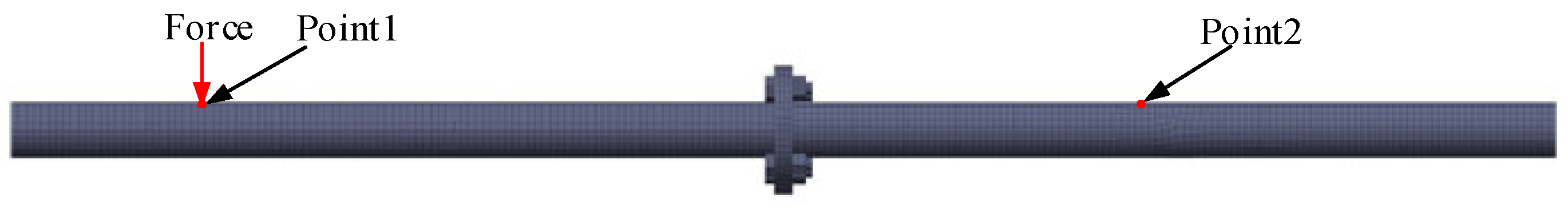
As depicted in Figure 10, the length of the straight pipe sections at both ends of the flange is 1 m. The model is meshed with hexahedral solid elements, and the element size is 10 mm, resulting in a total of 17,517 elements. Other property parameters of the pipe and boundary constraints are consistent with those in Section 4.1. DN65 flat-weld flanges (GB/9119-2000) are adopted, and the medium in the pipe is air.

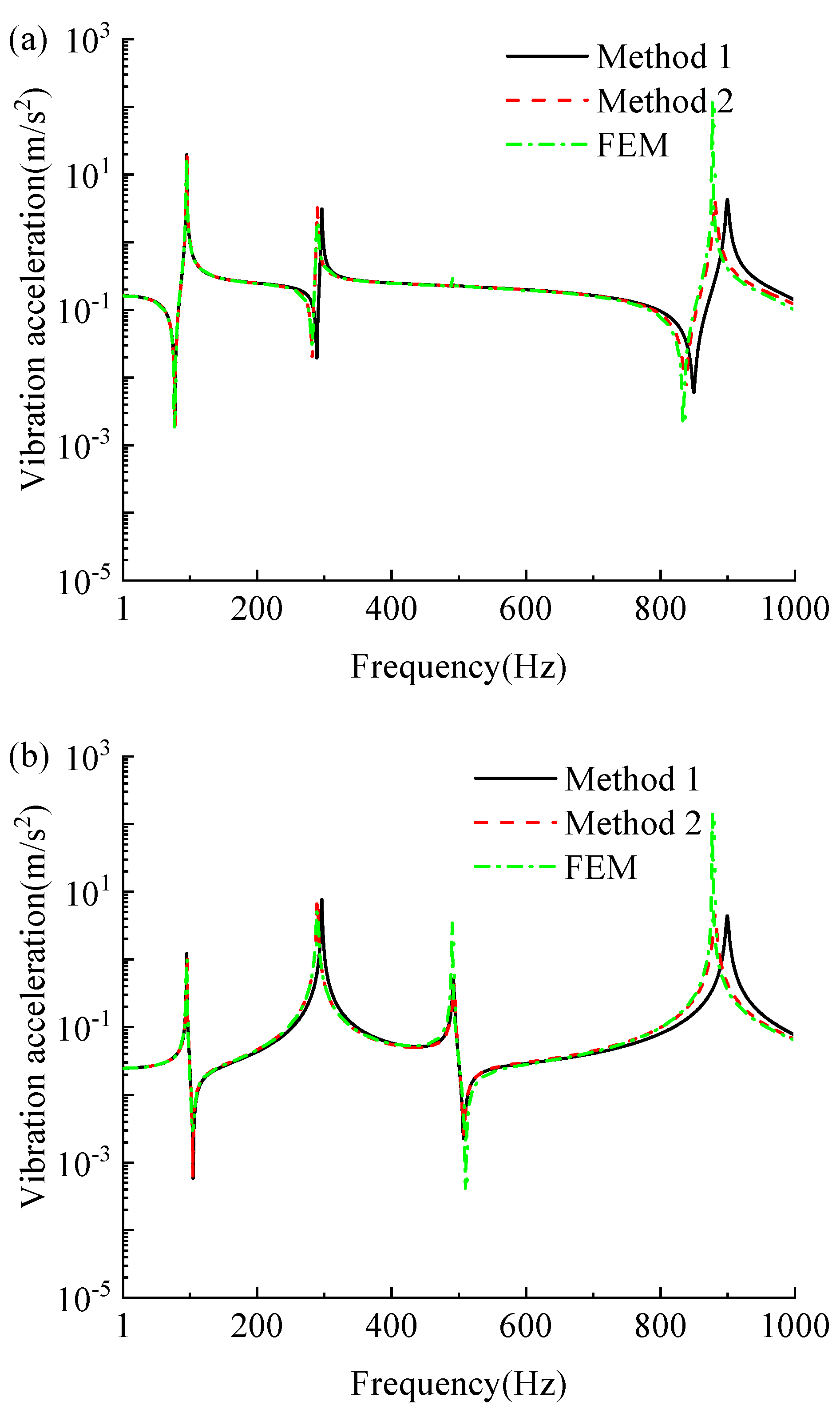
An external unit harmonic excitation force is applied at 0.2 m from the beginning of the pipe. Measurement point 1 is located at the excitation application point, and measurement point 2 is 0.5 m from the end. The acceleration responses of the pipe are solved using the two methods proposed in this paper and FEM. The comparison results are shown in Figure 11, and the corresponding first four natural frequencies are presented in

Table 2. Natural frequencies of pipe with flat-weld flanges.

Mode	1	2	3	4
Method 1	96.1 Hz	297.7 Hz	494.2 Hz	902.4 Hz
Method 2	96.3 Hz	291.0 Hz	490.4 Hz	884.0 Hz
FEM	95.8 Hz	290.9 Hz	491.8 Hz	880.1 Hz
Error based on Method 1	0.31%	2.34%	0.49%	2.53%
Error based on Method 1	0.52%	0.03%	0.28%	0.44%

. Due to the small mass and irregular shape of the flange connection bolts and nuts, subsequent calculations only consider their mass’s influence on the pipe’s vibration response, ignoring the moment of inertia.

Compared with the FEM results, the vibration acceleration response and natural frequencies calculated by Method 2 are basically consistent with those calculated by the FEM. In contrast, the error between Method 1 and the FEM results is relatively large. Based on the above analysis, the following conclusion can be drawn. When using the transfer matrix method to conduct overall calculation and analysis of pipe with flat-weld flanges, Method 2 has higher accuracy, and subsequent calculations mainly adopt Method 2.

4.3. Straight Pipe with Weld-Neck Flanges

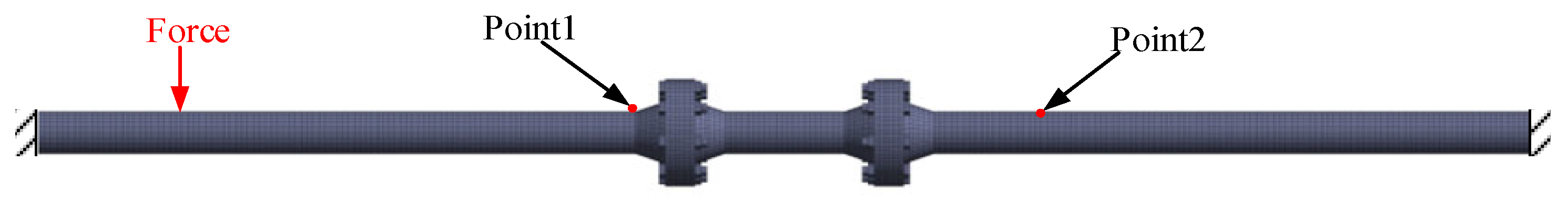
In this part, the correctness of the proposed transfer matrix calculation model for the weld-neck flange (CB/T 4327-2013) will be verified with the finite element model shown in Figure 12. The length of the straight pipes at both ends of the pipe is 1 m, while the length of the straight pipe in the middle is 0.2 m. The model is meshed with hexahedral solid elements, and the element size is 10 mm, resulting in a total of 25,812 elements. Other property parameters of the pipe are consistent with those in Section 4.1. DN65 weld-neck flanges are adopted, and the medium in the pipe is water. The bulk modulus of the water is K = 2.14 × 10⁹ Pa, and the density is ρl = 999 kg/m³.

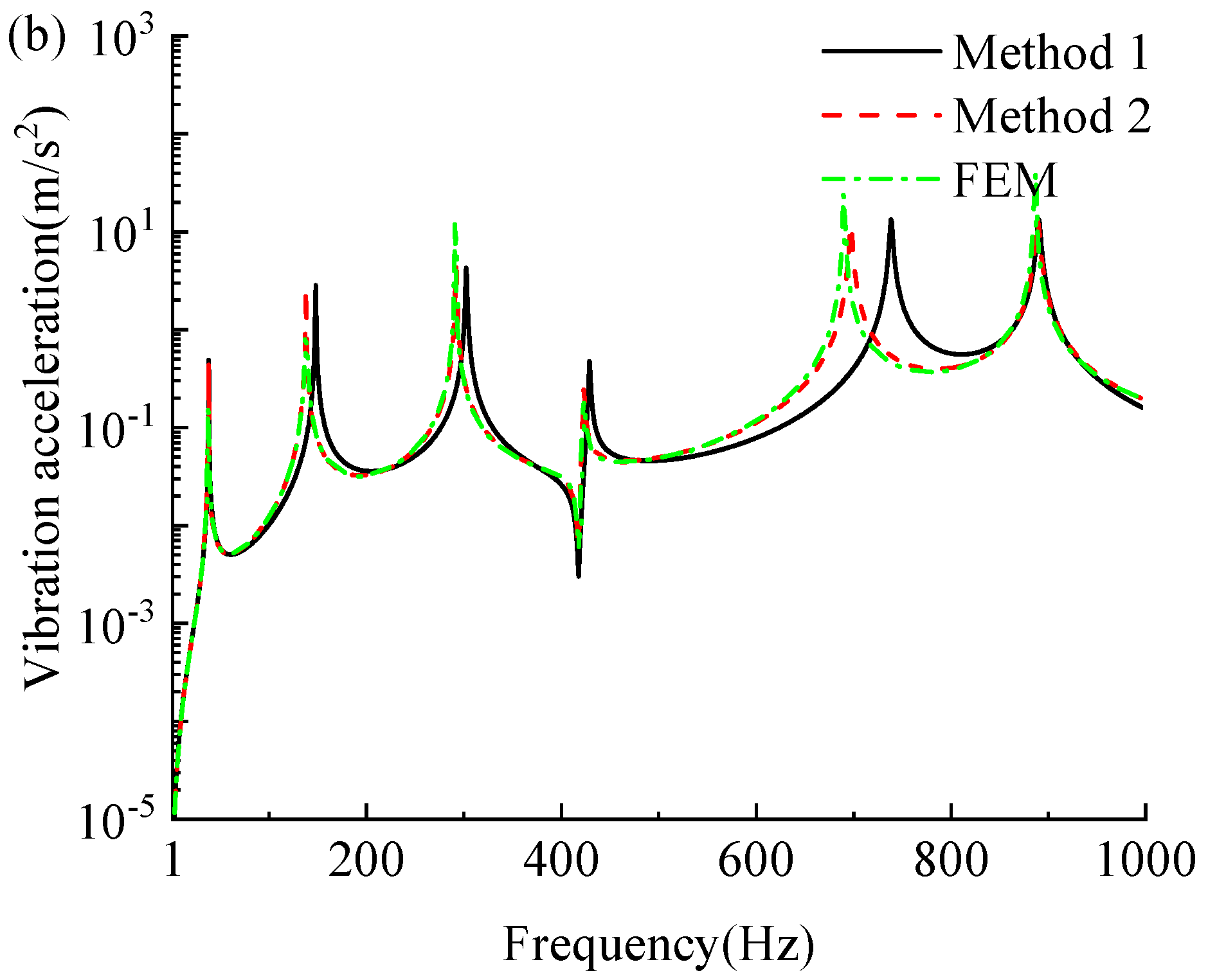
When calculating, both ends of the pipe are fixedly supported. At this time, the fluid pressure and the velocity variables of the pipe at the boundary are 0 and the boundary constraint matrix B is shown in Equation (14). An external unit harmonic excitation force is applied at 0.2 m from the beginning of the pipe. Measurement point 1 is 1 m away from the beginning of the pipe, and measurement point 2 is 0.8 m away from the end of the pipe. The acceleration responses of the pipe are solved using the two methods proposed in this paper and ANSYS, respectively. The comparison results are shown in Figure 13, and the corresponding first five natural frequencies are presented in

Table 3. Natural frequencies of the pipe with weld–neck flanges.

Mode	1	2	3	4	5
Method 1	38.6 Hz	148.6 Hz	303.7 Hz	430.4 Hz	741.1 Hz
Method 2	38.1 Hz	138.6 Hz	293.2 Hz	424.6 Hz	699.7 Hz
FEM	38.2 Hz	138.7 Hz	292.2 Hz	424.2 Hz	692.7 Hz
Error based on Method 1	1.05%	7.14%	3.94%	1.46%	6.99%
Error based on Method 1	0.26%	0.07%	0.34%	0.09%	1.01%

.

$$B=\left[\begin{array}{cccccccccccccc}0& 1& 0& 0& 0& 0& 0& 0& 0& 0& 0& 0& 0& 0\\ 0& 0& 1& 0& 0& 0& 0& 0& 0& 0& 0& 0& 0& 0\\ 0& 0& 0& 0& 1& 0& 0& 0& 0& 0& 0& 0& 0& 0\\ 0& 0& 0& 0& 0& 0& 1& 0& 0& 0& 0& 0& 0& 0\\ 0& 0& 0& 0& 0& 0& 0& 0& 1& 0& 0& 0& 0& 0\\ 0& 0& 0& 0& 0& 0& 0& 0& 0& 0& 1& 0& 0& 0\\ 0& 0& 0& 0& 0& 0& 0& 0& 0& 0& 0& 0& 1& 0\end{array}\right]$$

(14)

It can be seen that the pipe vibration acceleration response calculated by Method 2 is basically consistent with the FEM result throughout the calculation frequency range, which proves the correctness of this method. Method 1 is in good agreement with the FEM results before 500 Hz. After 500 Hz, with as the frequency increased, the error of the calculation results of Method 1 increased accordingly.

Through the above analysis, the following conclusion can be drawn. When the transfer matrix method is used to conduct the overall calculation and analysis of the pipe with weld-neck flanges, the accuracy of Method 2 is higher. Unlike Method 1, Method 2 can also calculate the vibration response on the flanges. Therefore, the subsequent calculations mainly adopt Method 2.

4.4. Experimental Verification of Pipe with Flanges

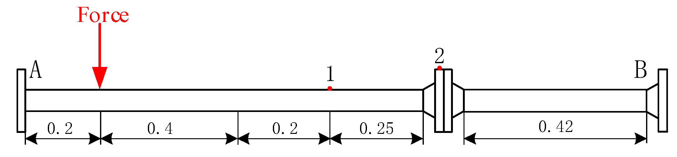
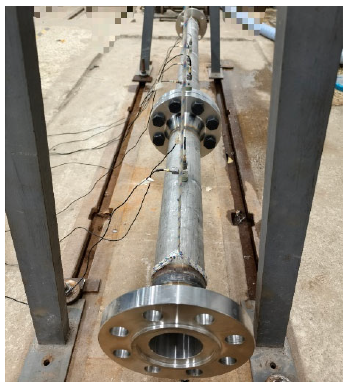
To verify the applicability of the method proposed in this paper on actual pipes, this section will further illustrate the application of the flange model and method described in this paper through complex pipes containing flat-weld flanges and weld-neck flanges. In the overall pipe model built in this experiment, weld-neck flanges are connected by bolts to simulate the pipe connection situation in actual engineering. The schematic of the pipe installation and the physical diagram of the experiment are shown in Figure 14 and Figure 15. In Figure 14, the A and B ends of the pipe are connected to the support by nylon ropes. At this time, the pipe is equivalent to free support, and its boundary constraint matrix B is shown in Equation (13). Points 1 and 2 represent the measurement points for the vibration acceleration of the pipe wall. The inner radius of the straight pipe is R = 0.0325 m, and the wall thickness is e = 0.005 m. The pipe material is structural steel, with Young’s modulus E = 1.90 × 10¹¹ Pa, density ρ_l =7850 kg/m³, and Poisson’s ratio ν = 0.3. We adopt DN65 weld-neck flanges and flat-weld flanges.

In this experiment, a force hammer (Model LC02-3A102, DongHua Testing Technology Co., Ltd., Jingjiang, China) delivers a vertical excitation to the pipe 0.20 m from end A while the pipe is initially at rest. The vibration response is recorded by a BK-4534BX accelerometer (Brüel & Kjær Sound & Vibration Measurement A/S, Nærum, Denmark), the position of which is indicated in Figure 14. The experimental data are collected and processed through the PULSE system. The comparison with the computational results of the method in this paper and the FEM is shown in Figure 16.

It can be seen from Figure 16 that the computational results of this method are in good agreement with the measurement results of the vibration experiment of the flanged pipe, which proves the correctness and effectiveness of this method in analyzing the vibration problems of such pipes.

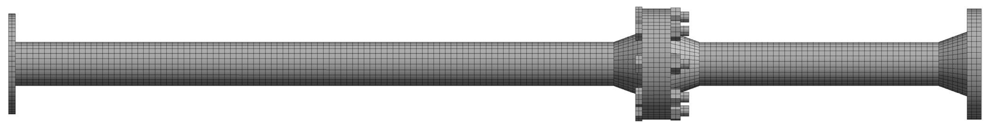
The finite element model of the experimental pipe is shown in Figure 17. The model is meshed with hexahedral solid elements, and the element size is 10 mm, resulting in a total of 52,689 elements.

Table 4. The mode shapes of the experimental pipe (air-filled).

Mode	Present	ANSYS
1
2

lists the modal shapes within the analysis frequency band of the experimental air-filled pipe. In this method, the dotted lines represent vibration modes, and the solid lines represent the original model. The modal vibration patterns of the pipe obtained by the two methods are basically the same, indicating that this method is highly accurate in calculating the vibration characteristics and inherent characteristics of pipes with flanges.

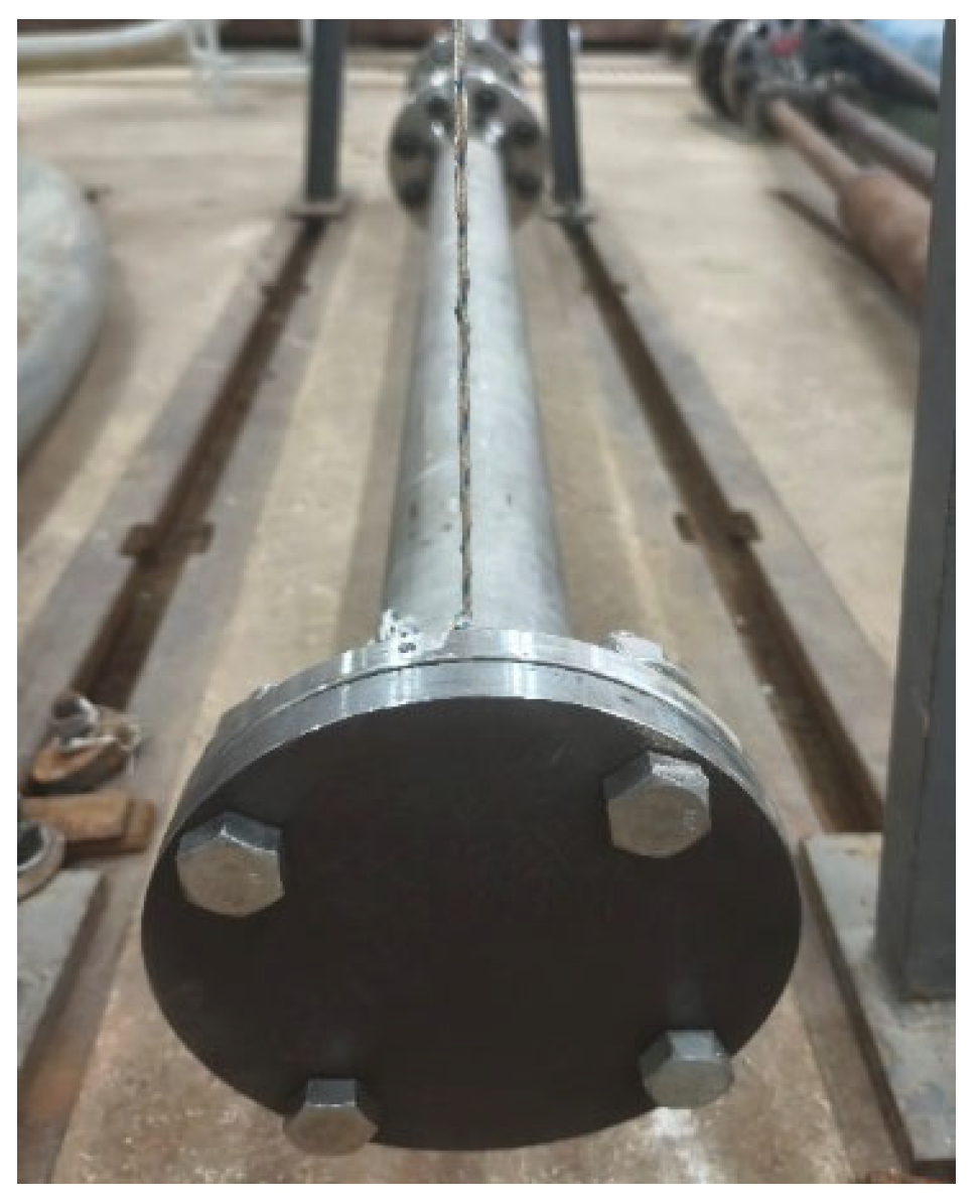
Consider the pipe filled with water. In the experiment, water is sealed in the pipe through blind plates. The blind plates at both ends of the pipe weighed 2.92 kg and 4.62 kg, respectively, as shown in Figure 18. The positions of the pipe vibration measurement points and the experimental process are the same as those in the air-filled pipe.

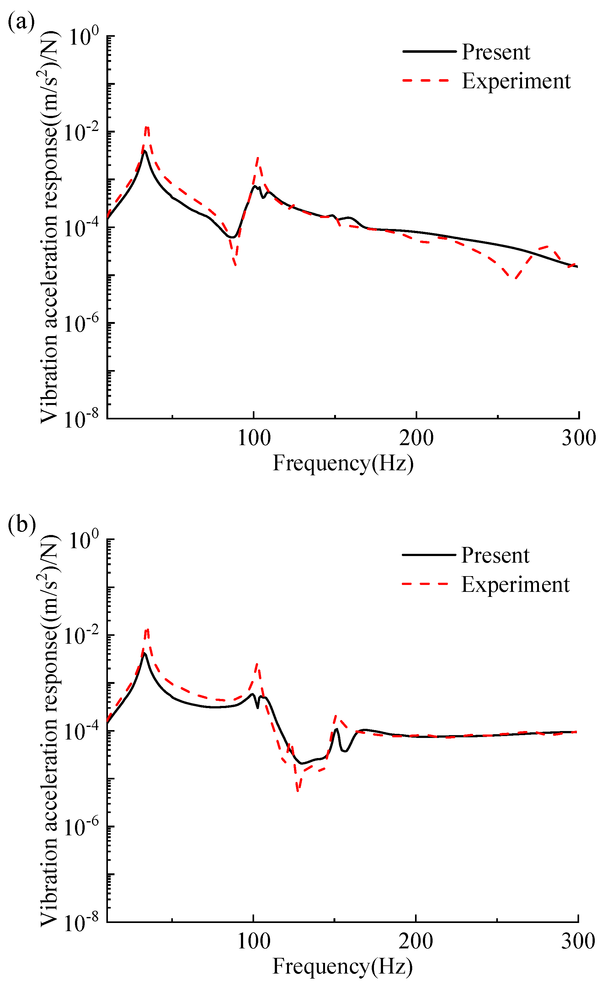
The vibration acceleration responses of the measurement points on the pipe are calculated by the method in this paper. The experimental results are shown in Figure 19. It can be seen that when the pipe is filled with water, the calculation results of the method in this paper are generally in good agreement with the experimental results but slightly worse than those of the air-filled pipe. The deviation between the two may mainly be caused by the following reasons: (a) The experimental results may be disturbed by factors not considered in the calculation, such as the acceleration sensor possibly sensing motion in other directions, and there may be parameter differences between the calculation and the experiment, such as Young’s modulus, etc.; (b) Due to reasons, such as gravity, installation, or welding processes, the pipe is not completely within the horizontal plane, and there is a certain amount of prestress, which can also cause errors; (c) This method does not consider the influence of flange gaskets on the vibration response of the pipe; (d) Although both ends of the pipe are connected to the supports by nylon ropes, the connection points are still not completely free.

4.5. Experimental Verification of Elbow Pipe with Flanges

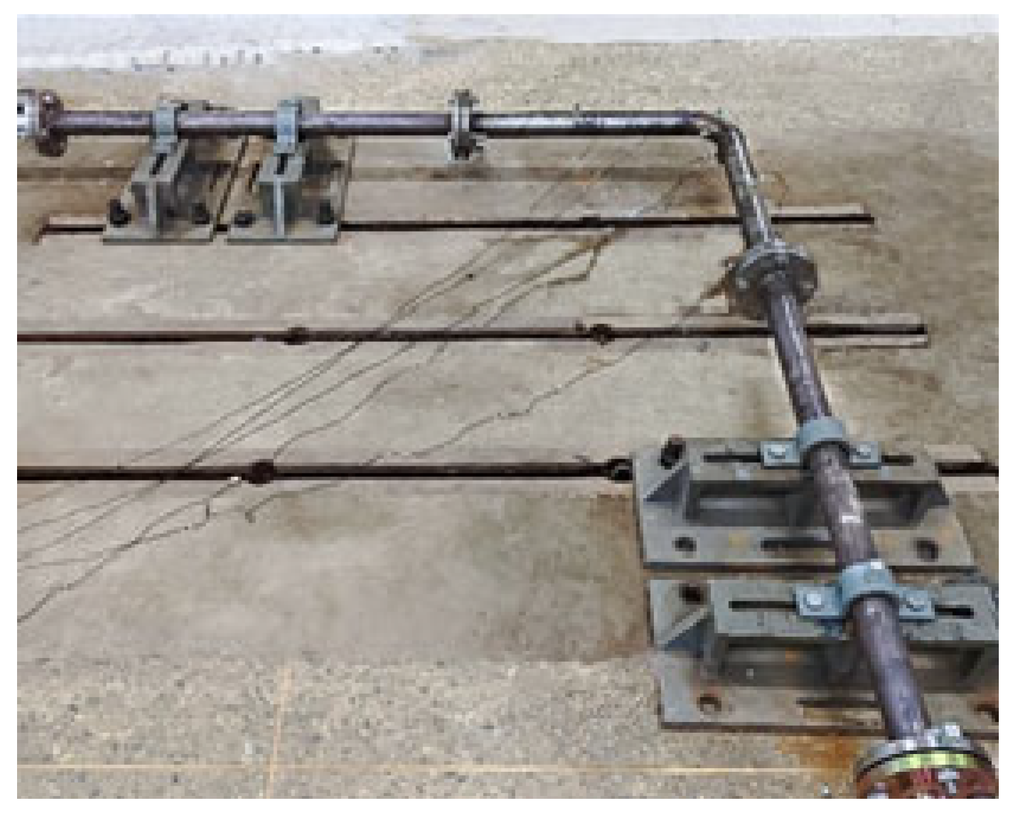
Validation of the applicability of the method proposed for complex pipelines and boundary conditions is conducted on the pipe shown in Figure 20. The pipe has an inner diameter of 52 mm, a wall thickness of 4 mm, and other sizes are shown in Figure 21. The pipe is filled with water. The material properties of the pipe are the same as those in Section 4.4. Both ends of the pipe are free, and the straight pipe sections at both ends of the elbow are connected to the base via clamps.

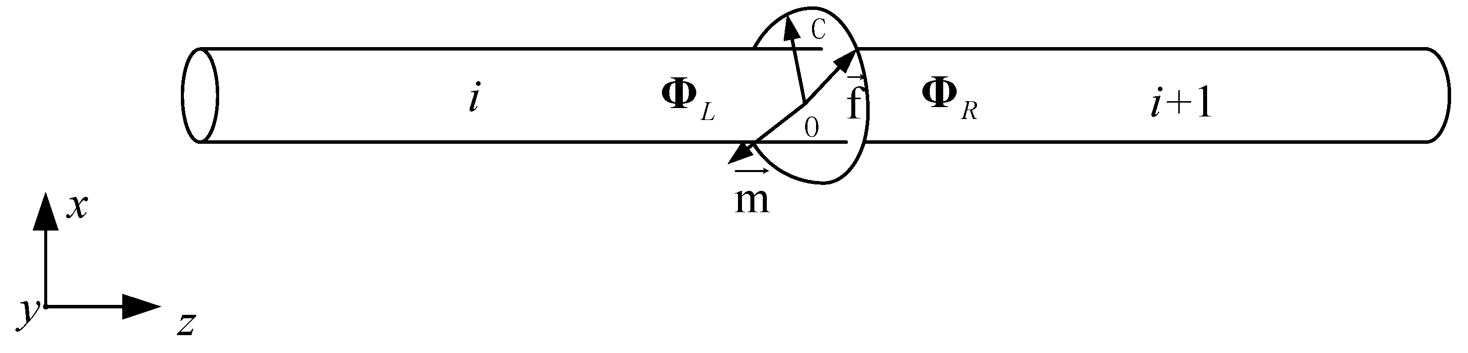
The transfer relationship between the state vectors of the left and right sides of the elastic support point of the pipe satisfies Φ_L = U_KΦ_R, where the transfer matrix of the elastic support point is as follows:

$${\mathbf{U}}_K=\left[\begin{array}{cccccccccccccc}1& 0& 0& 0& 0& 0& 0& 0& 0& 0& 0& 0& 0& 0\\ 0& 1& 0& 0& 0& 0& 0& 0& 0& 0& 0& 0& 0& 0\\ 0& 0& 1& 0& 0& 0& 0& 0& 0& 0& 0& 0& 0& 0\\ 0& 0& {\displaystyle \frac{k_z}{s}}& 1& 0& 0& 0& 0& 0& 0& 0& 0& 0& 0\\ 0& 0& 0& 0& 1& 0& 0& 0& 0& 0& 0& 0& 0& 0\\ 0& 0& 0& 0& {\displaystyle \frac{k_y}{s}}& 1& 0& 0& 0& 0& 0& 0& 0& 0\\ 0& 0& 0& 0& 0& 0& 1& 0& 0& 0& 0& 0& 0& 0\\ 0& 0& 0& 0& 0& 0& {\displaystyle \frac{k_{\theta x}}{s}}& 1& 0& 0& 0& 0& 0& 0\\ 0& 0& 0& 0& 0& 0& 0& 0& 1& 0& 0& 0& 0& 0\\ 0& 0& 0& 0& 0& 0& 0& 0& {\displaystyle \frac{k_x}{s}}& 1& 0& 0& 0& 0\\ 0& 0& 0& 0& 0& 0& 0& 0& 0& 0& 1& 0& 0& 0\\ 0& 0& 0& 0& 0& 0& 0& 0& 0& 0& {\displaystyle \frac{k_{\theta y}}{s}}& 1& 0& 0\\ 0& 0& 0& 0& 0& 0& 0& 0& 0& 0& 0& 0& 1& 0\\ 0& 0& 0& 0& 0& 0& 0& 0& 0& 0& 0& 0& {\displaystyle \frac{k_{\theta z}}{s}}& 1\end{array}\right]$$

(15)

where k_x, k_y, k_z, k_θx, k_θy, and k_θz represent the stiffness in each direction.

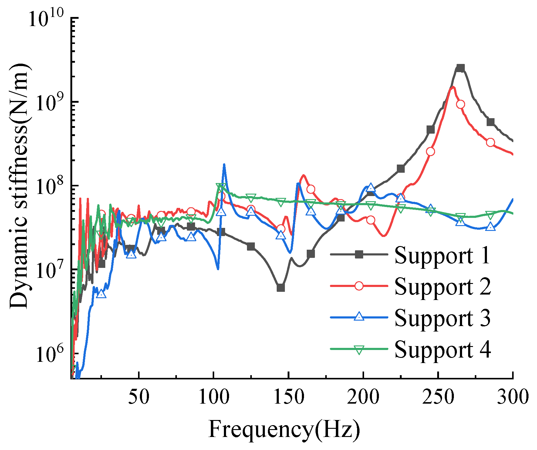
Before verification, it is necessary to measure the support stiffness in the experimental installation state. The vertical stiffness of each support is measured through experiments, as shown in Figure 22.

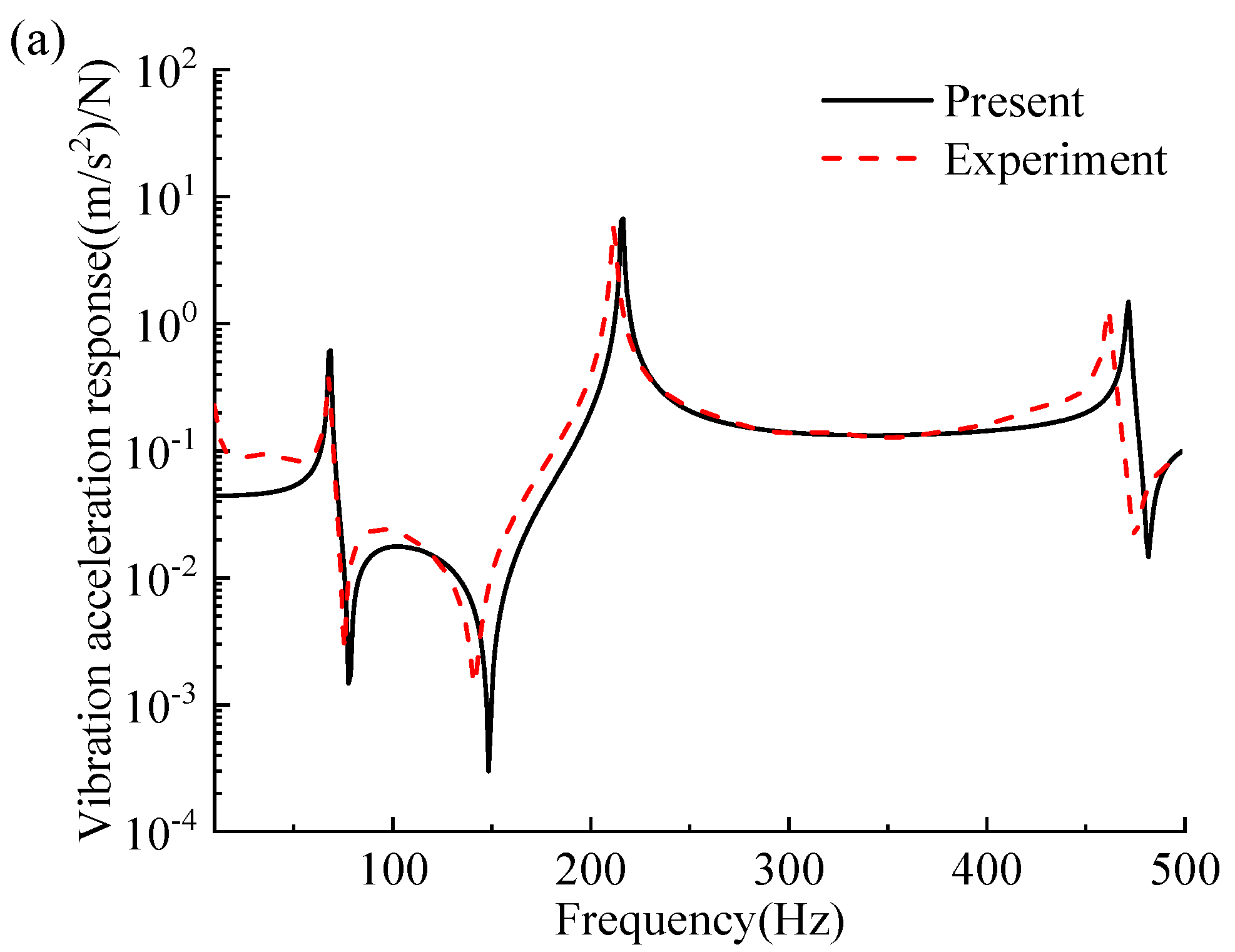
During the frequency response validation, the excitation and response measurement points of the pipe are shown in Figure 21. A comparison between the method proposed and the experimental results is shown in Figure 23. The results within the frequency range of 1~300 Hz exhibit agreement with the experimental data. There are deviations in certain frequency bands. The deviation may primarily be caused by the stiffness measured by the experiment, which has errors, and by the neglect of the influence of torsional stiffness. Overall, this indicates that this method proposed is feasible for predicting the vibration response characteristics of complex pipelines with actual application boundary conditions and flanges.

4.6. Dynamic Design of Branch Pipeline with Weld-Neck Flanges

The preceding mathematical models—including the transfer matrices for typical components (straight pipes, elbow pipes, and branch pipes), and the validated high-precision Method 2 for flange transfer matrices—enable accurate calculation of key dynamic parameters (natural frequencies, vibration responses, and modal shapes) of fluid-filled pipelines with complex components, like flanges. However, engineering practice demands more than prediction; it requires efficient optimizing designs to avoid resonance with external excitations (e.g., industrial pump frequencies) and enhance stability. To this end, this section will introduce the multi-objective particle swarm optimization algorithm to achieve the rapid optimization design of typical pipelines.

4.6.1. Selection of Optimization Objectives and Establishment of Optimization Models

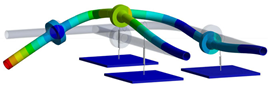
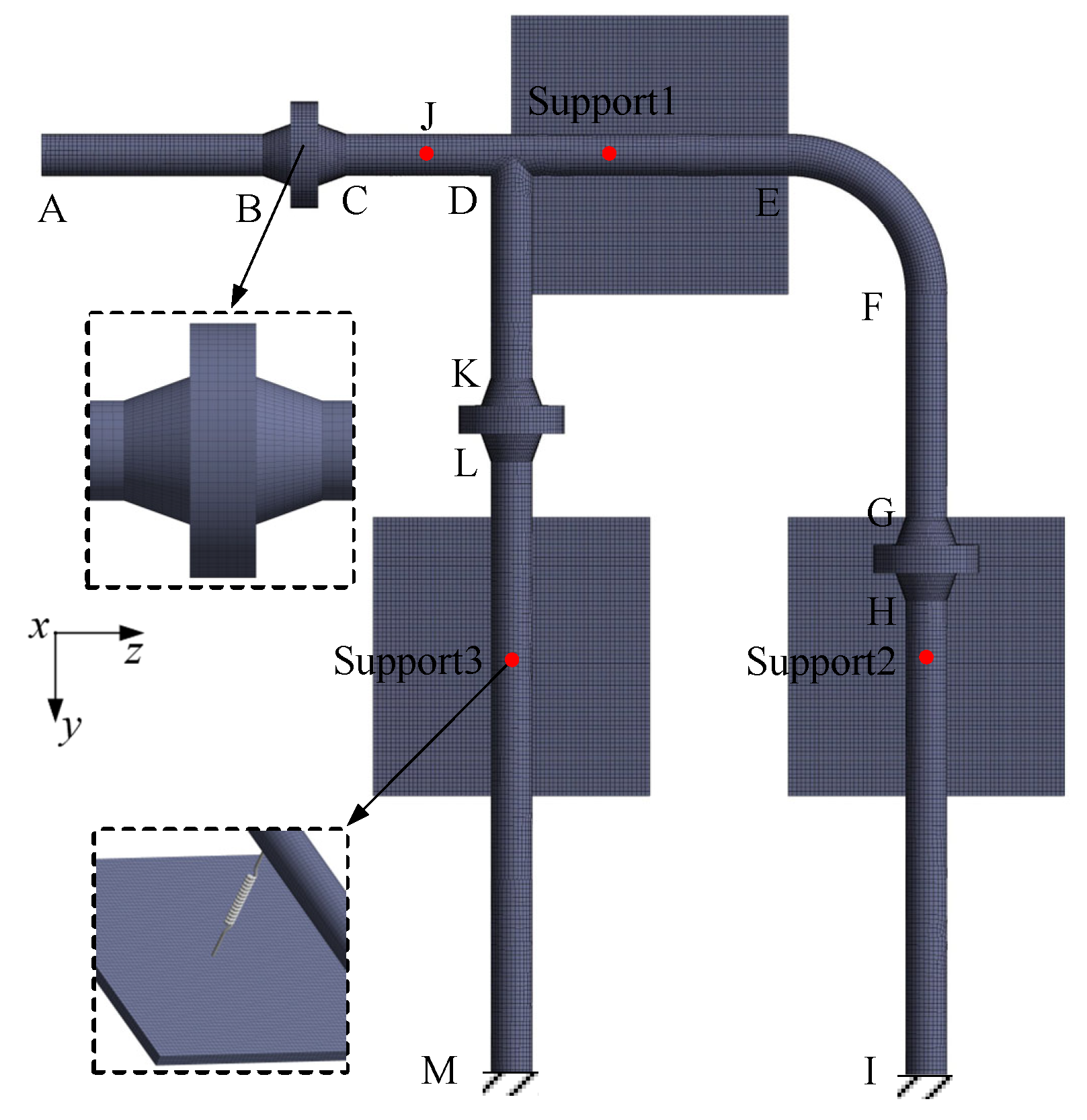
The pipeline finite element model for optimization is illustrated in Figure 24, where AB = FG = 0.4 m, CD = DK = 0.3 m, DE = 0.5 m, HI = 0.85 m, and LM = 1.1 m. The distance between support 1 and point D is 0.2 m, the distance between support 2 and point H is 0.1 m, and the distance between support 3 and point L is 0.35 m. The model is meshed with hexahedral solid elements, and the element size is 8 mm, resulting in a total of 200,869 elements. The parameters of the pipe material are consistent with those of the straight pipe in Section 4.1. The bending radius of the elbow pipe is 0.25 m, the inner radius of the pipe is 0.0325 m, and the wall thickness is 0.005 m. Both ends of pipeline I and M are fixed, while end A is free. The length, width, and thickness of the elastic plate are 0.5 m, 0.5 m, and 0.02 m, respectively. When calculating, the flexibility of the plate is considered. The origin impedance of the plate needs to be obtained through the FEM or experiments as the boundary condition of the transfer matrix method. In the finite element calculation, the four sides of the plate are fixed. The obtained origin impedance is shown in Figure 25. Combining the four-polo parameters of the spring, the point transfer matrix at the support can be obtained [20]. The initial values of the elastic support stiffness are all 1.3 × 10⁶ N/m, and the medium inside the pipe is water. When constructing the pipeline system model, considering that the bolts and flange holes have a relatively small impact on the overall dynamic characteristics, the simplified treatment is as follows: The flange plate of the weld-neck flange is equivalent to a straight pipe structure, and the flange connection holes and bolts are ignored.

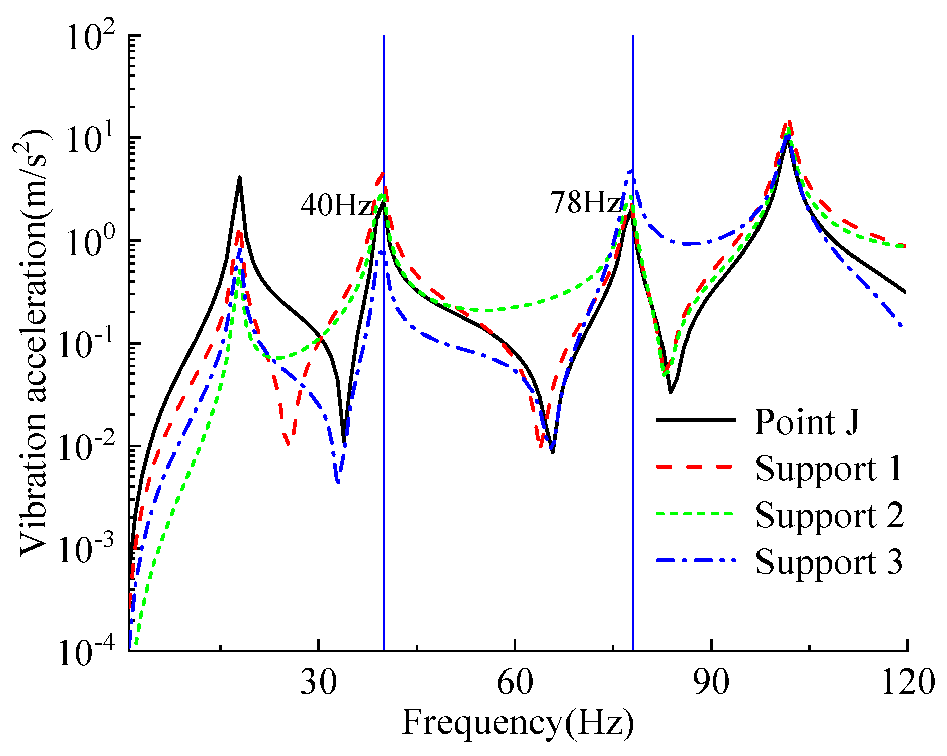
At point J, which is 0.2 m away from end C, an external harmonic excitation force of 10 N is applied. The acceleration responses of each measurement point in the pipeline are shown in Figure 26. Industrial current-carrying pipelines may be stimulated by water pumps during operation. Under normal circumstances, the rotational speed R_p of the water pump connected to the industrial flow-carrying pipeline is mostly within the range of 1500–3600 r/min, and the excitation base frequency corresponding to this rotational speed range is approximately 25–60 Hz. This paper assumes that the pipeline to be optimized is excited by a fundamental frequency of 40 Hz. In practical situations, in addition to the fundamental frequency vibration, the excitation source often generates certain excitation at integer multiples of its frequency. Therefore, the excitation effect of the excitation source at 80 Hz, which is twice the fundamental frequency, is considered. According to the frequency reserve requirements [21], the resonance domains of the two excitation frequencies can be calculated as 36–44 Hz and 72–88 Hz, respectively. It can be seen in Figure 26 that the second and third natural frequencies of the current-carrying pipeline both fall within the resonance range and need to be optimized. Therefore, in this paper, the optimization targets of the second and third natural frequencies are set at 48 Hz and 95 Hz, respectively.

4.6.2. Multi–Objective Particle Swarm Optimization Algorithm

In this paper, the second and third natural frequencies are taken as the optimization objectives and the support stiffness at the three supports are taken as optimization variables. The MOPSO algorithm is adopted to optimize the inherent characteristics of the pipeline system shown. We suppose that the variation range of the elastic support stiffness at each of the three positions is 10⁴–10⁷ N/m.

4.6.3. Optimize the Design Results

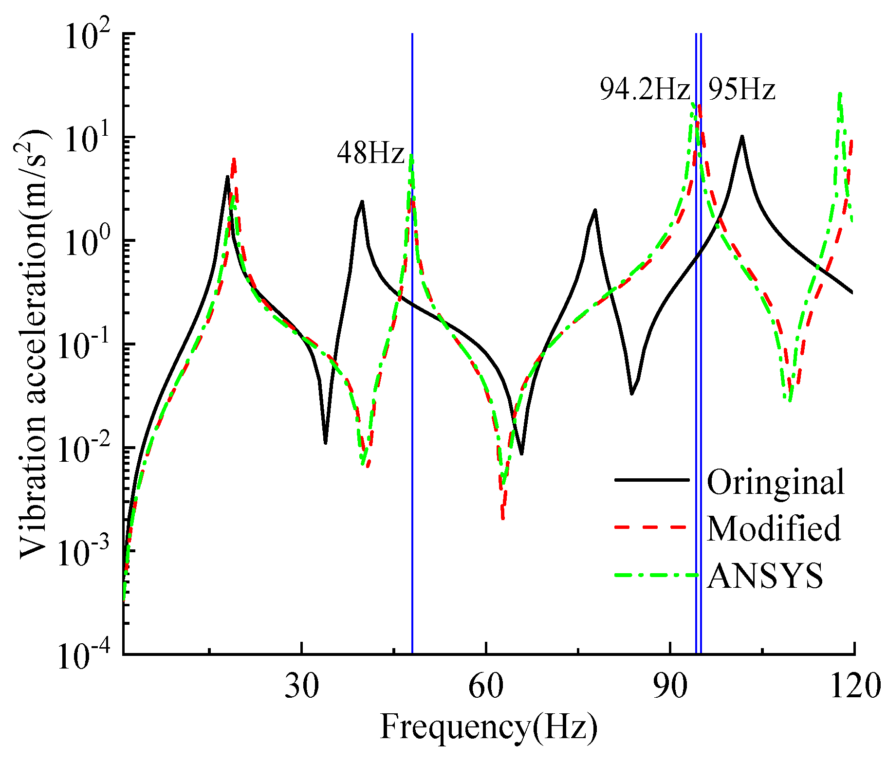
The MATLAB (R2019b Version) program is written based on the relationship between the independent variable and the objective function. Through the MOPSO algorithm, the optimal stiffness values of supports 1, 2, and 3 are calculated as 5.09 × 10⁶ N/m, 1 × 10⁴ N/m, and 7.99 × 10⁶ N/m, respectively. The optimal solution is substituted into this method for calculation, and a finite element model is established for simulation. During the finite element calculation, we fix the four sides of the support base. The acceleration responses of point J before and after the optimized configuration are shown in Figure 27. The second and third natural frequencies of the pipeline as calculated by simulation are 47.9 Hz and 94.2 Hz, respectively, and the errors between the theoretical optimization objective and the simulation results are 0.2% and 0.4%, respectively.

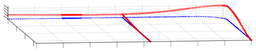
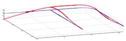
In the study of the pipeline modal shapes, the calculation results of the method in this paper and the first three pipeline modal shapes obtained by ANSYS are shown in

Table 5. The modal shapes of the optimized pipe.

Mode	Present	ANSYS
1
2
3

. In contrast, the vibration patterns and node distributions of this method are highly consistent, which fully verifies the accuracy and reliability of the method proposed in this paper in the analysis of the natural vibration patterns of complex pipeline systems.

The results show that the adopted method accurately achieves the optimal configuration goals of the second and third natural frequencies of the numerical model. Furthermore, by comparing these results with the finite element calculation results, the accuracy of this method in the optimization of natural frequencies is confirmed. Furthermore, it can be seen from Figure 27 that through the rational definition of target natural frequencies and structural optimization, the second and third modes of the pipeline system are effectively shifted away from the excitation frequency range of the connected equipment. This effectively suppresses the resonance and enhances the dynamic stability of the structure. In addition, the MOPSO algorithm is used to calculate 30 samples, with 50 iterations and a calculation time of 6 min 32 s. It balances optimization accuracy with computational efficiency. These outcomes demonstrate the practical significance and engineering value of the method.

5. Conclusions

In this paper, the fluid-filled ship piping system is taken as the research object, and transfer matrix models of the pipeline system considering flat-weld flanges and weld-neck flanges are established. The pipe model is verified through the methods of FEM and experiments, expanding the application scope of the transfer matrix method in calculating the fluid–structure coupling dynamics of pipeline systems. Meanwhile, the MOPSO algorithm is adopted to optimize the design of the specific pipeline. The main conclusions are as follows:

• Two calculation methods for the transfer matrix of flat-weld flanges and weld-neck flanges are proposed. The verification shows that Method 2 has higher accuracy. In the verification of the flanged pipe model, the vibration acceleration response and natural frequency calculated by Method 2 are basically consistent with the FEM results. Method 1 is in good agreement with the FEM results at low frequencies, but the error is significant at high frequencies.
• The experimental results show that the vibration test results are in agreement with the prediction of the method in this paper, and the deviation between the two can be explained by predictable reasons. This kind of difference is acceptable in the preliminary engineering design and estimation.
• The modal shapes of straight pipe and branch pipe with flanges calculated by the proposed method are in good agreement with the ANSYS results, which verifies the practicability and correctness of TMM in solving the inherent characteristics of such pipeline systems.
• The MOPSO algorithm is adopted to optimize the design of the branch pipeline with weld-neck flanges. Considering the flexibility of the support base, the second and third natural frequencies are taken as optimization objectives, and the support stiffness at the three support points is taken as the optimization variable. The optimization result enables the pipeline’s natural frequency to avoid the excitation frequency and prevent resonance successfully. The accuracy of the method in natural frequency optimization is confirmed by finite element model simulation. Moreover, the computational time is 6 min 32 s, demonstrating good computational efficiency while maintaining optimization accuracy.