Hybrid Obstacle Avoidance Algorithm Based on IAPF and MPC for Underactuated Multi-USV Formation

Abstract

In this paper, we propose a hybrid algorithm that integrates an improved artificial potential field method (IAPF), model predictive control (MPC), and an extended state observer (ESO) to address the obstacle avoidance problem in multi-unmanned surface vehicle (Multi-USV) formations, including both dynamic and static obstacles, as well as navigation through narrow waterways. Initially, the virtual structure method was applied for formation control. Next, the traditional potential field method was enhanced by employing a saturated attractive potential field and a partitioned repulsive potential field, which improve formation stability and obstacle avoidance accuracy in complex environments. The extended state observer was then employed to estimate and compensate for unknown system dynamics and external disturbances from the marine environment in real time, improving system robustness. On this basis, by leveraging the multi-step predictive optimization capabilities of model predictive control, the proposed algorithm dynamically adjusts control inputs based on the desired trajectories generated from potential field forces, which ensures the stability of formation control and effective obstacle avoidance. The simulation results demonstrate that the proposed algorithm effectively avoids both dynamic and static obstacles in multi-unmanned surface vehicle formations and enables successful navigation through narrow waterways by altering the formation.

1. Introduction

As marine operational tasks grow increasingly complex and diverse, the capabilities of a single unmanned vessel are not able to meet the demands of such tasks. The multi-unmanned surface vehicle cooperative formation system, which capitalizes on advantages such as distributed decision-making, resource coordination, and environmental adaptability, has emerged as a key technology for addressing the limitations of single-vessel operations [1,2]. Through the exchange of information and cooperative control among multiple agents, the system facilitates task scalability, enhances operational efficiency, and improves robustness. It demonstrates substantial application value in complex scenarios, including deep-sea exploration, emergency rescue, and marine area monitoring [3,4]. However, during mission execution, unmanned surface vehicle formations may encounter various dynamic and static obstacles (such as islands and reefs, no-sailing zones, offshore platforms) and restricted waters (such as narrow waterways), often affecting navigational safety. These obstacles not only undermine the stability of the formation system but also place greater demands on the robustness of collaborative control. Therefore, stability control and collaborative obstacle avoidance techniques, including formation maintenance and reconfiguration, for multi-unmanned surface vehicle formations in complex environments have recently emerged as a key research focus in relevant domains.

Formation control and obstacle avoidance strategies for unmanned surface vehicles primarily include the virtual structure method [5], leader–follower method [6], artificial potential field method [7,8], and model predictive control [9,10,11]. To fully leverage and integrate the technical advantages of various methods while overcoming the performance limitations of a single approach, a series of hybrid strategies have been proposed. Typically, hybrid algorithms combining artificial potential fields and model predictive control capitalize on the rapid real-time obstacle avoidance offered by the artificial potential field method and the global optimization and constraint-handling capabilities of model predictive control. This combination effectively mitigates the issues of local optima and path oscillations inherent in the use of a single potential field method and has been widely adopted for obstacle avoidance in diverse scenarios [12,13,14,15,16,17,18,19,20,21,22,23]. For example, Xinwei Wang et al. [14] enhanced the traditional potential field method by incorporating angular velocity constraints and time information, thereby enabling the generation of high-quality short-term reference trajectories and effectively preventing obstacle collisions. They then employed model predictive control to accurately track these reference trajectories, ensuring precise control of a single vessel in complex environments. Yujie Huang et al. [15] developed an autonomous obstacle avoidance controller for multi-unmanned vessel formations by establishing communication priorities and a unidirectional topology, integrating hypothetical and balanced state spaces into the distributed model predictive control algorithm, and combining it with the artificial potential field method to improve the safety of the vessel formation. Zhibo He et al. [16] introduced a motion planning method that combines model predictive strategies with artificial potential fields, transforming the ship motion planning problem into a multi-constrained nonlinear optimization problem. This method effectively addresses collision avoidance for a single vessel in complex intersection scenarios while adhering to collision avoidance rules. Haibin Li et al. [17] adopted a separation-type mathematical model for a vessel and conducted a comprehensive analysis of its motion characteristics. They designed a collision avoidance decision-making framework based on the artificial potential field method and model predictive control. This approach effectively mitigates the issues of local optima and bow oscillations commonly encountered during path planning using the artificial potential field method. Beixi Ning et al. [18] incorporated dynamic adjustment factors and a buffer layer structure into the traditional artificial potential field method, integrating it with distributed model predictive control. They developed a cost function that evaluates path optimization based on safety, stability, and energy consumption, ensuring the smoothness and stability of the formation’s path when navigating around static obstacles. Han et al. [19] combined nonlinear model predictive control with path planning, collision avoidance, and motion control coordination, introducing an adaptive steering constraint Theta* algorithm. They also employed an enhanced potential field method to address various obstacle types, effectively resolving the issue of safe navigation for vessels in complex environments. The authors of [20,21] proposed collision avoidance decision-making frameworks for ships based on enhanced artificial potential fields and nonlinear model predictive control, in accordance with COLREG rules. These approaches effectively ensure both collision avoidance and path tracking for a single vessel, while improving the system’s computational efficiency and maneuverability in dynamic environments. The existing research on hybrid APF-MPC mainly focuses on two aspects: one is dynamic and static obstacle-avoidance for an individual vessel [14,16,17,19,20,21], and the other is obstacle-avoidance for multi-USV formations in open waters [15,18,22,23]. However, studies addressing obstacle avoidance control for unmanned vessel formations in complex environments such as narrow waters are relatively fewer. Moreover, existing methods do not address the problem of multi-unmanned boat formation maintenance, especially in narrow or obstacle-intensive waters, where it is difficult to coordinate formation and obstacle avoidance, leading to path oscillation and formation destabilization [24,25].

The paper presents a formation-based obstacle avoidance control strategy for multi- unmanned surface vehicles operating in complex environments subject to perturbations such as wind, waves, and currents. The proposed approach integrates an enhanced artificial potential field method, model predictive control, and an extended state observer. The expected values and disturbance estimates derived from the improved artificial potential field and the extended state observer, respectively, are used to dynamically adjust the inputs to the model predictive controller. This strategy not only ensures successful avoidance of both static and dynamic obstacles by the multi-unmanned surface vehicle formation but also enables smooth navigation through narrow waterways by adapting the formation, effectively mitigating oscillations, and avoiding entrapment in local optima.

(1)

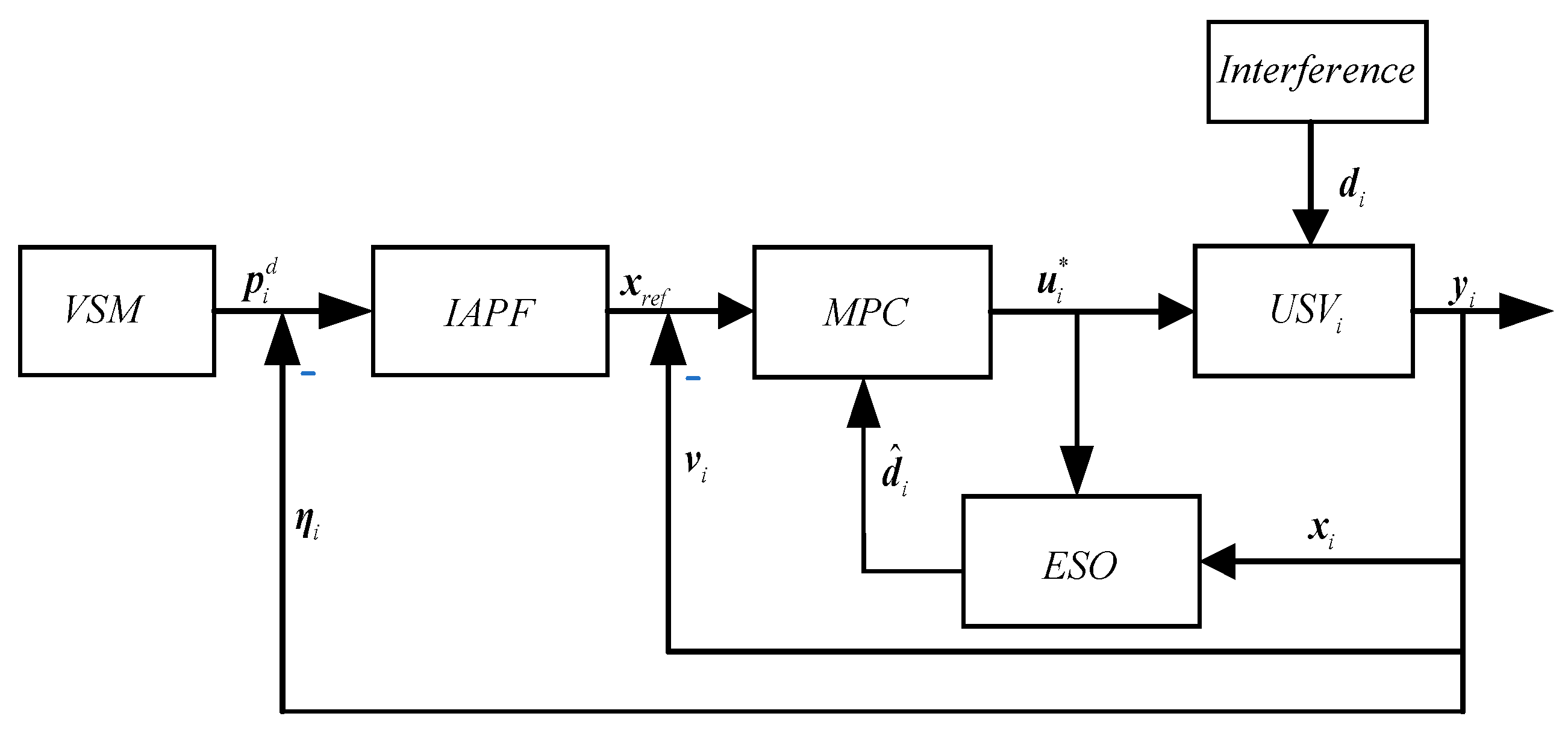
A saturated gravitational potential field is introduced for narrow waterways to prevent formation instability due to excessive gravitational forces. Additionally, a partitioned repulsive potential field is implemented, dynamically adjusting the potential field function based on the distance between unmanned surface vehicles and a waterway boundary, thereby ensuring effective obstacle avoidance within the unmanned surface vehicle formation.

(2)

By leveraging the multi-step prediction capability of model predictive control, the controller is designed based on the expected values provided by the enhanced artificial potential field and the disturbance estimates derived from the extended state observer, ensuring that the state and velocity vectors of the USVs in the formation asymptotically converge to the desired values.

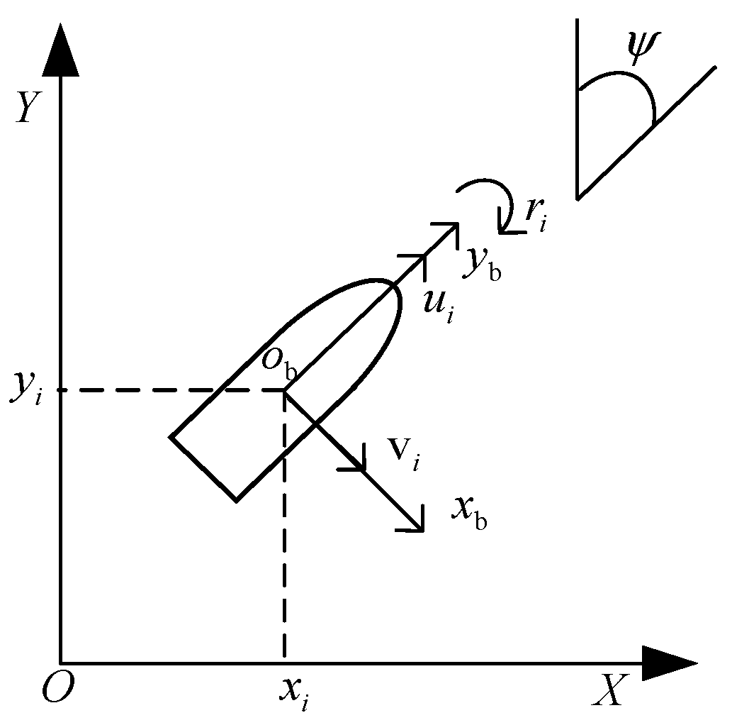
2. Problem Statement

A coordinate system, illustrated in Figure 1, is established according to the terminology bulletin published by the Society of Naval Architects and Marine Engineers. Here, $XOY$ represents the geodetic coordinate system, while $x_{\mathit{b}}{o}_{\mathit{b}}{y}_{\mathit{b}}$ corresponds to the body-fixed coordinate system.

The kinematic and dynamic models for the $i-th$ unmanned surface vehicle can be expressed as follows:

$$\left\{\begin{array}{l}{\stackrel{·}{\mathit{\eta }}}_i={\mathit{J}}_i({\psi }_i){\mathit{v}}_i\\ {\mathit{M}}_i{\stackrel{·}{\mathit{v}}}_i+{\mathit{C}}_i({\mathit{v}}_i){\mathit{v}}_i+{\mathit{D}}_i({\mathit{v}}_i){\mathit{v}}_i={\mathit{\tau }}_i+{\mathit{\tau }}_{iw}+{\mathit{f}}_i({\mathit{v}}_i)\end{array}\right.$$

(1)

In the kinematic model, ${\mathit{\eta }}_i={\left[\begin{array}{ccc}{x}_i& y_i& {\psi }_i\end{array}\right]}^{\mathrm{T}}$ represents the position and heading angle of the $US{V}_i$ in the inertial coordinate system. Specifically, $\left(x_i,y_i\right)$ denotes the position vector in the fixed coordinate system, ${\psi }_i\in \left(-\pi ,\pi \right]$ is the heading angle of the $US{V}_i$, and the components of ${\mathit{v}}_i={\left[\begin{array}{ccc}{u}_i& {\mathrm{v}}_i& r_i\end{array}\right]}^{\mathrm{T}}$ correspond to the longitudinal velocity, lateral velocity, and yaw rate in the body-fixed coordinate system, respectively. The transformation matrix ${\mathit{J}}_i$ is defined as follows:

$${\mathit{J}}_i({\psi }_i)=\left[\begin{array}{ccc}\cos {\psi }_i& -\sin {\psi }_i& 0\\ \sin {\psi }_i& \cos {\psi }_i& 0\\ 0& 0& 1\end{array}\right]$$

(2)

In the dynamic model, the mass matrix is denoted by ${\mathit{M}}_i=diag\left\{m_i^u,m_i^{\mathit{v}},m_i^r\right\}\in {ℝ}^{3\times 3}$, the Coriolis and centripetal matrix by ${\mathit{C}}_i\left({\mathit{v}}_i\right)\in {ℝ}^{3\times 3}$, and the damping matrix by ${\mathit{D}}_i\left({\mathit{v}}_i\right)\in {ℝ}^{3\times 3}$. The control input is expressed as ${\mathit{\tau }}_i={\left[{\mathit{\tau }}_i^u,0,{\mathit{\tau }}_i^r\right]}^{\mathrm{T}}$. External environmental disturbances in the form of wind, waves, and currents are represented by ${\mathit{\tau }}_{iw}={\left[{\mathit{\tau }}_{iw}^u,{\mathit{\tau }}_{iw}^{\mathit{v}},{\mathit{\tau }}_{iw}^r\right]}^{\mathrm{T}}$. Model uncertainty is denoted by ${\mathit{f}}_i\left({\mathit{v}}_i\right)={\left[f_{iu},f_{i\mathit{v}},f_{ir}\right]}^{\mathrm{T}}$, which comprises the perturbations $f_{iu}\left(\cdot \right)=-m_{22}{\mathrm{v}}_i{r}_i+d_{11}{u}_i$, $f_{i\mathrm{v}}\left(\cdot \right)=m_{11}{u}_i{r}_i+d_{22}{\mathrm{v}}_i$, and $f_{ir}\left(\cdot \right)=$$\left(m_{22}-m_{11}\right)u_i{\mathrm{v}}_i+d_{33}{r}_i$.

The primary objective of this study is to achieve formation control and obstacle avoidance for multi-unmanned vehicle systems subjected to system uncertainties, external environmental disturbances, and control input constraints. The USVs first navigate forward in a predetermined geometric formation. When a narrow waterway is detected, a formation reconstruction algorithm is triggered automatically. The algorithm will switch the formation to a compact one that adapts to the waterway’s width, allowing the USVs to navigate through the restricted area. After passing through the narrow waterway, the USVs either revert to their original formation or switch to a new one suited for the task. Moreover, a virtual structure strategy is employed to accomplish the formation, ensuring that the state vector ${\mathit{\eta }}_i$ and velocity vector ${\mathit{v}}_i$ of the $US{V}_i$ asymptotically track the desired trajectories ${\mathit{\eta }}_{id}$ and ${\mathit{v}}_{id}$; that is, $\underset{t\to \infty }{\lim }‖{\mathit{\eta }}_i-{\mathit{\eta }}_{id}‖=0$ and $\underset{t\to \infty }{\lim }‖{\mathit{v}}_i-{\mathit{v}}_{id}‖=0$.

3. Main Results

This paper presents a hybrid control framework as shown in Figure 2, which combines an improved artificial potential field, model predictive control, and an extended state observer to enable formation keeping and obstacle avoidance for USVs. The improved artificial potential field module plans collision-free reference trajectories and supplies the model predictive controller with path and velocity set-points. Subject to input constraints, this controller performs multi-step prediction and real-time optimization to generate optimal control commands for coordinated motion and safe navigation. The extended state observer estimates and compensates for unmodeled dynamics and external maritime disturbances.

3.1. Controller Design

3.1.1. Formation Control Based on Virtual Structure

Inspired by works in [26,27], the virtual structural particles are modeled as a second-order system with both kinematic and dynamic characteristics:

$$\left\{\begin{array}{l}{\dot{p}}_i=q_i\\ {\dot{q}}_i=u_i\end{array}\right.$$

(3)

In this context, $p_i$ and $q_i$ represent the position and velocity vectors of the virtual structural particle of the $US{V}_i$ in the fixed coordinate system, while $u_i$ denotes its control input.

To ensure the convergence of the position and velocity of the virtual structural particle to the desired values, the control law is designed as follows:

$$u_i=c_1\left(p_i^d-p_i\right)+c_2\left(q_i^d-q_i\right)$$

(4)

where $c_1$ and $c_2$ are the position and velocity control coefficients, respectively, and $p_i^d$ and $q_i^d$ represent the desired position and velocity of the virtual structural particle of the $US{V}_i$ in the fixed coordinate system.

Substituting Equation (4) into Equation (3) yields a second-order linear system:

$${\ddot{p}}_i+c_2{\dot{p}}_i+c_1{p}_i=c_2{\dot{p}}_i^d+c_1{p}_i^d$$

(5)

The position and velocity of the formation reference point in the fixed coordinate system are given by $p_r$ and $q_r$. The desired position and velocity of the virtual structural particle of the unmanned vehicle in the fixed coordinate system are given by

$$\left\{\begin{array}{l}{p}_i^d=p_r+\mathit{R}\left({\psi }_r\right)L{r}_i\\ q_i^d=q_r+\stackrel{·}{\mathit{R}}\left({\psi }_r\right)L{r}_i+\mathit{R}\left({\psi }_r\right)\dot{L}{r}_i\end{array}\right.$$

(6)

where $R\left({\psi }_r\right)=\left[\begin{array}{cc}\cos {\psi }_r& -\sin {\psi }_r\\ \sin {\psi }_r& \cos {\psi }_r\end{array}\right]$ represents the coordinate transformation matrix, ${\psi }_r$ denotes the heading angle of the formation reference point, and $L=\left[\begin{array}{cc}l& 0\\ 0& l\end{array}\right]$ is the formation scaling factor. The term $r_i$ represents the relative position between the virtual structural particle of the $US{V}_i$ and the formation reference point. If $r_i$ remains constant, the formation is maintained; if $r_i$ varies, formation reconfiguration is achieved.

3.1.2. Improved Artificial Potential Field Method

In complex environments such as narrow waterways, when multiple unmanned vehicles approach a target point, the traditional attractive potential field increases infinitely [24]. This can lead to over-adjustment and oscillation of the unmanned vehicles, making smooth arrival at the target difficult. Therefore, this study adopts a saturated attractive potential field to limit the attraction near the target. When an unmanned vehicle is within a predefined saturation threshold distance from the target, the attraction increases linearly. If the distance exceeds this threshold, the attraction reaches its maximum value and remains constant. This design prevents an infinite increase in attraction, ensuring that the unmanned vehicle can decelerate smoothly and accurately reach its target position. The details of the design are outlined below.

The improved expression of the attractive potential field is as follows:

$$U_{\mathrm{att}}\left({\mathit{q}}_i\right)=\left\{\begin{array}{cc}{\displaystyle \frac{1}{2}}{k}_{\mathrm{att}}{‖{\mathit{q}}_i-{\mathit{q}}_{\mathrm{goal}}‖}^2,& ‖{\mathit{q}}_i-{\mathit{q}}_{\mathrm{goal}}‖\le \rho \\ {\displaystyle \frac{1}{2}}{k}_{att}{\rho }^2,& ‖{\mathit{q}}_i-{\mathit{q}}_{\mathrm{goal}}‖>\rho \end{array}\right.$$

(7)

Here, $\rho$ denotes the saturation distance threshold.

The attractive force $F_{\mathrm{att}}\left({\mathit{q}}_i\right)$ is obtained by computing the negative gradient of the attractive potential field $U_{\mathrm{att}}\left({\mathit{q}}_i\right)$:

$$F_{\mathrm{att}}\left({\mathit{q}}_i\right)=-\nabla U_{\mathrm{att}}\left({\mathit{q}}_i\right)=\left\{\begin{array}{cc}-k_{\mathrm{att}}\left({\mathit{q}}_i-{\mathit{q}}_{\mathrm{goal}}\right),& ‖{\mathit{q}}_i-{\mathit{q}}_{\mathrm{goal}}‖\le \rho \\ 0,& ‖{\mathit{q}}_i-{\mathit{q}}_{\mathrm{goal}}‖>\rho \end{array}\right.$$

(8)

Within the vicinity of target $\rho$, the attractive force increases as the distance decreases, vanishing at the target point. Beyond this region, the attractive force is zero, implying that the potential field no longer influences unmanned vehicles at greater distances. Introducing a saturation mechanism enables the attractive potential field to retain an appropriate magnitude near the target, thereby preventing unmanned vehicles from undergoing severe oscillations or overcompensating.

In narrow waterways and other complex environments, USVs must avoid collisions with both surrounding obstacles and neighboring craft. Accordingly, the formation control algorithm must maintain the desired geometry while guaranteeing navigational safety in obstacle and inter-vehicle collision avoidance. To enable a USV formation to transit narrow waterways without becoming trapped in local optima, we propose a partitioned repulsive potential field method that ensures safe clearance of boundaries and obstacles. The channel is divided into discrete zones, and the repulsive force is dynamically scaled according to each USV’s distance from the boundaries, thereby enabling smooth obstacle avoidance within confined waters.

Figure 3 depicts typical narrow waterways, including ship locks and canals. Let the channel have a total width $2d$ and be divided symmetrically about its centerline. A repulsive potential field is imposed along both boundaries to confine the maneuvering space of USVs and guarantee safe transit through the central corridor. The formulation of the repulsive potential field, and thus the resultant repulsive force, is identical for USVs located between the upper boundary and centerline and those between the centerline and lower boundary.

Based on the partitioning of the repulsive potential field, the waterway is divided into three distinct zones: the safety zone, the buffer zone, and the danger zone. The safety zone, denoted as Zone $(0-d_{\mathrm{n}})$, corresponds to the region in which the USV can safely traverse the central section of the waterway, with minimal or no repulsive force. The buffer zone, denoted as Zone $(d_{\mathrm{n}}-d_{\mathrm{m}})$, is the area in which the USV gradually approaches the waterway boundaries, and the repulsive force increases to prevent the vehicle from getting too close. Finally, in the danger zone, denoted as Zone $(d_{\mathrm{m}}-d)$, the repulsive force escalates sharply to ensure that the USV quickly moves away from the boundary region.

The expression for the improved repulsive potential field is as follows:

$$U_{\mathrm{rep}-\mathrm{top}}\left({\mathit{q}}_i\right)=\left\{\begin{array}{l}0,‖{\mathit{q}}_i-{\mathit{q}}_{\mathrm{b}1}‖\ge d_1\\ {\displaystyle \frac{1}{2}}{k}_{\mathrm{rep}1}{\left({\displaystyle \frac{1}{d_1}}-{\displaystyle \frac{1}{‖{\mathit{q}}_i-{\mathit{q}}_{\mathrm{b}1}‖}}\right)}^2,d_2\le ‖{\mathit{q}}_i-{\mathit{q}}_{\mathrm{b}1}‖<d_1\\ {\displaystyle \frac{1}{2}}{k}_{\mathrm{rep}2}{\left({\displaystyle \frac{1}{‖{\mathit{q}}_i-{\mathit{q}}_{\mathrm{b}1}‖}}-{\displaystyle \frac{1}{d_2}}\right)}^2,‖{\mathit{q}}_i-{\mathit{q}}_{\mathrm{b}1}‖<d_2\end{array}\right.$$

(9)

In this expression, $k_{\mathrm{rep}1}$ and $k_{\mathrm{rep}2}$ are the coefficients of the repulsive potential field, ${\mathit{q}}_{\mathrm{b}1}$ represents the position vector of the upper boundary of the narrow waterway, $d_1$ is the distance threshold of the buffer zone, and $d_2$ is the distance threshold of the danger zone.

The repulsive force $F_{\mathrm{rep}}\left({\mathit{q}}_i\right)$ is obtained by computing the negative gradient of the repulsive potential field $U_{\mathrm{rep}}\left({\mathit{q}}_i\right)$:

$$F_{\mathrm{rep}-\mathrm{top}}\left({\mathit{q}}_i\right)=-\nabla U_{\mathrm{rep}-\mathrm{top}}\left({\mathit{q}}_i\right)=\left\{\begin{array}{l}0,‖{\mathit{q}}_i-{\mathit{q}}_{\mathrm{b}1}‖\ge d_1\\ k_{\mathrm{rep}1}\left({\displaystyle \frac{1}{d_1}}-{\displaystyle \frac{1}{‖{\mathit{q}}_i-{\mathit{q}}_{\mathrm{b}1}‖}}\cdot {\displaystyle \frac{1}{{‖{\mathit{q}}_i-{\mathit{q}}_{\mathrm{b}1}‖}^2}}\right),d_2\le ‖{\mathit{q}}_i-{\mathit{q}}_{\mathrm{b}1}‖<d_1\\ k_{\mathrm{rep}2}\left({\displaystyle \frac{1}{‖{\mathit{q}}_i-{\mathit{q}}_{\mathrm{b}1}‖}}-{\displaystyle \frac{1}{d_2}}\right)\cdot {\displaystyle \frac{1}{{‖{\mathit{q}}_i-{\mathit{q}}_{\mathrm{b}1}‖}^2}},‖{\mathit{q}}_i-{\mathit{q}}_{\mathrm{b}1}‖<d_2\end{array}\right.$$

(10)

The resultant potential field is formed through the superposition of the attractive and repulsive potential fields, denoted as $U_{\mathrm{total}}\left({\mathit{q}}_{\mathit{i}}\right)=U_{\mathrm{att}}\left({\mathit{q}}_i\right)+{\displaystyle \sum U_{\mathrm{rep}}\left({\mathit{q}}_i\right)}$. The behavior of the $US{V}_i$ within this field is governed by the resultant force. By taking the negative gradient of the resultant potential field, we can obtain the resultant force acting on the $US{V}_i$: $F_{\mathrm{total}}\left({\mathit{q}}_i\right)=F_{\mathrm{att}}\left({\mathit{q}}_i\right)+{\displaystyle \sum F_{\mathrm{rep}}\left({\mathit{q}}_i\right)}$. This resultant force $F_{\mathrm{total}}\left({\mathit{q}}_i\right)$ provides the $US{V}_i$ with comprehensive navigation and obstacle avoidance information, which will serve as the desired input for model predictive control to optimize the vehicle’s motion trajectory.

3.1.3. Extended State Observer

This study utilizes the extended state observer as the central mechanism for disturbance estimation and compensation. Originally proposed by Professor Jingqing Han [28], the extended state observer serves as a critical component of the active disturbance rejection control framework. In contrast to the traditional Luenberger observer, it offers several key advantages: it does not require an accurate system model, it can estimate unknown disturbances as additional states, and it allows for straightforward parameter tuning, primarily by selecting the observer’s bandwidth. These features make the extended state observer particularly effective for unmanned surface vehicle systems in marine environments, where obtaining precise dynamic parameters is challenging and external disturbances are complex and unpredictable.

First, the mathematical model of $US{V}_i$ in (1) is rewritten as follows:

$${\mathit{M}}_i^{*}{\mathit{v}}_i=-{\mathit{C}}_i^{*}\left({\mathit{v}}_i\right){\mathit{v}}_i-{\mathit{D}}_i^{*}\left({\mathit{v}}_i\right){\mathit{v}}_i+{\mathit{\tau }}_i+{\mathit{d}}_i$$

(11)

where ${\mathit{M}}_i^{*}$, ${\mathit{C}}_i^{*}$, and ${\mathit{D}}_i^{*}$ represent nominal values that can be derived using computational fluid dynamics or empirical methods. ${\mathit{d}}_i={\mathit{\tau }}_{iw}+f_i\left({\mathit{v}}_i\right)$ represents the unknown dynamics of the USV, including external environmental disturbances, internal model uncertainties, and an uncertain inertia matrix.

Inspired by the work in [29], a second-order extended state observer is proposed to estimate the unknown terms in the system:

$$\left\{\begin{array}{l}{\stackrel{·}{\widehat{\overline{\mathit{v}}}}}_i=-{\mathit{K}}_1^{\mathit{v}}\left({\widehat{\overline{\mathit{v}}}}_i-{\overline{\mathit{v}}}_i\right)+{\mathit{M}}_i^{*-1}{\overline{\mathit{\tau }}}_i+{\widehat{\overline{\mathit{\sigma }}}}_i\\ {\stackrel{·}{\widehat{\overline{\mathit{\sigma }}}}}_i=-{\mathit{K}}_2^{\mathit{v}}\left({\widehat{\overline{\mathit{v}}}}_i-{\overline{\mathit{v}}}_i\right)\end{array}\right.$$

(12)

Here, ${\mathit{K}}_1^{\mathit{v}},{\mathit{K}}_2^{\mathit{v}}\in {ℝ}_{+}^{3\times 3}$ represents the diagonal observation gain matrix, while ${\widehat{\overline{v}}}_i,{\widehat{\overline{\sigma }}}_i$ indicates the estimated value of ${\overline{\mathit{v}}}_i,{\overline{\mathit{\sigma }}}_i$. ${\overline{\sigma }}_i={\left[{\left(m_i^{u*}\right)}^{-1}{\overline{f}}_{iu},{\left(m_i^{r*}\right)}^{-1}{\overline{f}}_{ir}\right]}^{\mathrm{T}}\in {ℝ}^2$, $M_i^{*}=diag\left\{m_i^{u*},m_i^{r*}\right\}\in {ℝ}^{2\times 2}$, and ${\overline{\tau }}_i={\left[{\tau }_i^u,{\tau }_i^r\right]}^{\mathrm{T}}\in {ℝ}^2$.

Let ${\widetilde{\overline{\mathit{v}}}}_i={\widehat{\overline{\mathit{v}}}}_i-{\overline{\mathit{v}}}_i$ and ${\widetilde{\overline{\mathit{\sigma }}}}_i={\widehat{\overline{\mathit{\sigma }}}}_i-{\overline{\mathit{\sigma }}}_i$ denote the estimation errors. Through the use of Equations (11) and (12), the estimation errors of the extended state observer can be expressed as follows:

$$\left\{\begin{array}{l}{\dot{\widetilde{\overline{\mathit{v}}}}}_i=-{\mathit{K}}_1^{\mathit{v}}{\widetilde{\overline{\mathit{v}}}}_i+{\widetilde{\overline{\mathit{\sigma }}}}_i\\ {\dot{\widetilde{\overline{\mathit{\sigma }}}}}_i=-{\mathit{K}}_2^{\mathit{v}}{\widetilde{\overline{\mathit{v}}}}_i-{\dot{\overline{\mathit{\sigma }}}}_i\end{array}\right.$$

(13)

To facilitate the subsequent stability analysis of the extended state observer, the following assumption is made:

 Assumption 1: 

The derivative of the nonlinear function ${\mathit{d}}_{ik}\left(\cdot \right)$, denoted by ${\dot{\mathit{d}}}_{ik}\left(\cdot \right),k=u,\mathrm{v},r$ , is bounded and satisfies the condition given in Equation (14).

$$\left|{\dot{\mathit{d}}}_{ik}\left(\cdot \right)\right|\le {\mathit{d}}_{ik}^{*},k=u,\mathrm{v},r$$

(14)

where ${\mathit{d}}_{ik}^{*}\in {ℝ}_{+}$. Since the control input of the USV is bounded, its velocity must also be bounded, which justifies Assumption 1.

To meet the real-time control requirements imposed on the USV and enable integration with model predictive control, the continuous extended state observer is discretized as follows:

$$\left\{\begin{array}{l}{\widehat{\overline{\mathit{v}}}}_{i,k+1}={\widehat{\overline{\mathit{v}}}}_{ik}+T_s\left[-{\mathit{K}}_1^{\mathit{v}}\left({\widehat{\overline{\mathit{v}}}}_{ik}-{\overline{\mathit{v}}}_{ik}\right)+{{\mathit{M}}_i^{*}}^{-1}{\overline{\mathit{\tau }}}_{ik}+{\widehat{\overline{\sigma }}}_{ik}\right]\\ {\widehat{\overline{\mathit{\sigma }}}}_{i,k+1}={\widehat{\overline{\mathit{\sigma }}}}_{ik}+T_s\left[-{\mathit{K}}_2^{\mathit{v}}\left({\widehat{\overline{\mathit{v}}}}_{ik}-{\overline{\mathit{v}}}_{ik}\right)\right]\end{array}\right.$$

(15)

In this case, $T_s$ represents the sampling period and is set to 0.1 s. Within the nominal model control framework, the disturbance rejection control law based on the extended state observer is formulated as

$${\overline{\mathit{\tau }}}_i={\mathit{M}}_i^{*}\left(-{\mathit{K}}_3{z}_{i1}-{\mathit{K}}_4\int z_{i1}dt+{\mathit{v}}_{id}-{\widehat{\overline{\mathit{\sigma }}}}_i\right)$$

(16)

where ${\mathit{K}}_3$ and ${\mathit{K}}_4$ represent the diagonal control gain matrix, $z_{i1}={\overline{\mathit{v}}}_i-{\mathit{v}}_{id}$ represents the velocity tracking error of the $US{V}_i$, and ${\mathit{v}}_{id}$ represents the desired velocity of the $US{V}_i$.

3.1.4. Model Predictive Control

Model predictive control, an advanced optimal control framework, offers significant advantages in handling multivariable coupled systems and receding horizon prediction. Its inherent adaptability and robustness make it well suited to complex marine environments, and its constraint-handling capability is indispensable in practice [30]. Building on the disturbance and model information furnished by the extended state observer in Section 3.1.3, we design a model predictive controller to drive the vessels of the multi-USV formation toward velocity consensus through optimal control inputs.

To satisfy the computational demands of real-time maritime operation without degrading obstacle avoidance performance, the controller is implemented in discrete time. Specifically, the continuous dynamic model (11) is discretized with a sampling period $T_s$ using the forward Euler method, yielding the following discrete-time representation:

$${\mathit{v}}_{\mathit{i}}\left(k+1\right)=\left(\mathit{I}-{\mathit{M}}_i^{*-1}{T}_s\left({\mathit{C}}_i^{*}+{\mathit{D}}_i^{*}\right)\right){\mathit{v}}_i\left(k\right)+{\mathit{M}}_i^{*-1}{T}_s{\mathit{\tau }}_i\left(k\right)+{\mathit{M}}_i^{*-1}{T}_s{\mathit{d}}_i\left(k\right)$$

(17)

By selecting ${\mathit{x}}_{i\mathit{v}}\left(k\right)={\left[{\mathit{v}}_i\left(k\right),{\mathit{\tau }}_i\left(k-1\right)\right]}^T$ to be the state vector and using the increment of $\Delta {\mathit{u}}_{i\tau }\left(k\right)={\tau }_i\left(k\right)-{\tau }_i\left(k-1\right)$ as the control input, we can derive the state-space model of the control system as follows:

$${\mathit{x}}_{iv}\left(k+1\right)={\mathit{A}}_{iv}{\mathit{x}}_{iv}\left(k\right)+{\mathit{B}}_{iv}\Delta {\mathit{u}}_{i\tau }\left(k\right)+{\mathit{E}}_{iv}{\mathit{d}}_i\left(k\right)$$

(18)

$${\mathit{y}}_{iv}\left(k\right)={\mathit{C}}_{iv}{\mathit{x}}_{iv}\left(k\right)$$

(19)

In this context, ${\mathit{A}}_{iv}=\left[\begin{array}{cc}{\mathit{I}}_3-{\mathit{M}}_i^{*-1}{T}_s\left({\mathit{C}}_i^{*}+{\mathit{D}}_i^{*}\right)& {\mathit{M}}_i^{*-1}{T}_s\\ 0_3& {\mathit{I}}_3\end{array}\right]$, $\mathit{B}=\left[\begin{array}{c}{\mathit{M}}_i^{*-1}{T}_s\\ {\mathit{I}}_3\end{array}\right]$, ${\mathit{E}}_{iv}=\left[\begin{array}{c}{\mathit{M}}_i^{*-1}Ts\\ 0_{3\times 1}\end{array}\right]$, and ${\mathit{y}}_{iv}$ constitute the output vector, ${\mathit{C}}_{iv}=\left[\begin{array}{cc}{\mathit{I}}_3& 0_3\end{array}\right]$. The recursive expression for the predicted state vector ${\mathit{x}}_{iv}$ is given by

$${\mathit{x}}_{iv}\left(k+1|k\right)={\mathit{A}}_{iv}{\mathit{x}}_{iv}\left(k|k\right)+{\mathit{B}}_{iv}\Delta {\mathit{u}}_{i\tau }\left(k|k\right)+{\mathit{E}}_{iv}{\mathit{d}}_i\left(k|k\right)$$

(20)

$$\begin{array}{ll}{\mathit{x}}_{iv}\left(k+2|k\right)& ={{\mathit{A}}_{iv}}^2{\mathit{x}}_{iv}\left(k|k\right)+{\mathit{A}}_{iv}{\mathit{B}}_{iv}\Delta {\mathit{u}}_{i\tau }\left(k|k\right)+\\ & {\mathit{B}}_{iv}\Delta {\mathit{u}}_{i\tau }\left(k+1|k\right)+\left({\mathit{A}}_{iv}{\mathit{E}}_{iv}+{\mathit{E}}_{iv}\right){\mathit{d}}_i\left(k|k\right)\end{array}$$

(21)

$$\begin{array}{ll}& \dots \\ {\mathit{x}}_{iv}(k+N_p|k)=& {\mathit{A}}_{iv}^{N_p}{\mathit{x}}_{iv}(k|k)+{\displaystyle \sum _{j=0}^{N_p-1}{\mathit{A}}_{iv}^{N_p-1-j}}{\mathit{B}}_{iv}\Delta {\mathit{u}}_{i\tau }(k+j|k)+\\ & {\displaystyle \sum _{j=0}^{N_p-1}{\mathit{A}}_{iv}^j}{\mathit{E}}_{iv}{\mathit{d}}_i(k|k)\end{array}$$

(22)

Similarly, the recursive formula for the predicted output vector ${\mathit{y}}_{iv}$ is given by

$${\mathit{y}}_{iv}\left(k+1|k\right)={\mathit{C}}_{iv}{\mathit{A}}_{iv}{\mathit{x}}_{iv}\left(k|k\right)+{\mathit{C}}_{iv}{\mathit{B}}_{iv}\Delta {\mathit{u}}_{i\tau }\left(k|k\right)+{\mathit{C}}_{iv}{\mathit{E}}_{iv}{\mathit{d}}_i\left(k|k\right)$$

(23)

$$\begin{array}{c}{\mathit{y}}_{iv}\left(k+2|k\right)={\mathit{C}}_{iv}{{\mathit{A}}_{iv}}^2{\mathit{x}}_{iv}\left(k|k\right)+{\mathit{C}}_{iv}{\mathit{A}}_{iv}{\mathit{B}}_{iv}\Delta {\mathit{u}}_{i\tau }\left(k|k\right)+\\ {\mathit{B}}_{iv}\Delta {\mathit{u}}_{i\tau }\left(k+1|k\right)+{\mathit{C}}_{iv}\left({\mathit{A}}_{iv}{\mathit{E}}_{iv}+{\mathit{E}}_{iv}\right){\mathit{d}}_i\left(k|k\right)\end{array}$$

(24)

$$\begin{array}{ll}& \dots \\ {\mathit{y}}_{iv}(k+N_p|k)=& {\mathit{C}}_{iv}{\mathit{A}}_{iv}^{N_p}{\mathit{x}}_{iv}(k|k)+{\displaystyle \sum _{j=0}^{N_p-1}{\mathit{C}}_{iv}{\mathit{A}}_{iv}^{N_p-1-j}}{\mathit{B}}_{iv}\Delta {\mathit{u}}_{i\tau }(k+j|k)+\\ & {\displaystyle \sum _{j=0}^{N_p-1}{\mathit{C}}_{iv}{\mathit{A}}_{iv}^j}{\mathit{E}}_{iv}{\mathit{d}}_i(k|k)\end{array}$$

(25)

Based on the recursive relationship above, the following prediction equations are used to characterize the relationship between the predicted output sequence and the control increment sequence:

$${\mathit{Y}}_{iv}=\mathit{\Phi }{\mathit{x}}_{iv}+\mathit{\Gamma }\Delta {\mathit{U}}_{i\tau }+\mathit{\Psi }{\mathit{d}}_i$$

(26)

where ${\mathit{Y}}_{iv}={\left[{\mathit{y}}_{iv}\left(k+1|k\right),{\mathit{y}}_{iv}\left(k+2|k\right),\dots ,{\mathit{y}}_{iv}\left(k+Np|k\right)\right]}^T$, $\Delta {\mathit{U}}_{i\tau }={\left[\Delta {\mathit{u}}_{i\tau }\left(k|k\right),\Delta {\mathit{u}}_{i\tau }\left(k+1|k\right),\dots ,\Delta {\mathit{u}}_{i\tau }\left(k+Nc-1|k\right)\right]}^T$, $\mathit{\Phi }=\left[{\mathit{C}}_{iv}{\mathit{A}}_{iv},{\mathit{C}}_{iv}{\mathit{A}}_{iv}^2,\dots ,{\mathit{C}}_{iv}{\mathit{A}}_{iv}^{Np}\right]$, $\mathit{\Gamma }=\left[\begin{array}{cccc}{C}_{iv}{B}_{iv}& 0_3& \dots & 0_3\\ C_{iv}{A}_{iv}{B}_{iv}& C_{iv}{B}_{iv}& \dots & 0_3\\ ⋮& ⋮& \ddots & ⋮\\ C_{iv}{A}_{iv}^{Np-1}{B}_{iv}& C_{iv}{A}_{iv}^{Np-2}{B}_{iv}& \dots & C_{iv}{A}_{iv}^{Np-Nc}{B}_{iv}\end{array}\right]$, and

$\mathit{\Psi }={\left[{\mathit{C}}_{iv}{\mathit{E}}_{iv},{\mathit{C}}_{iv}{\mathit{A}}_{iv}{\mathit{E}}_{iv}+{\mathit{C}}_{iv}{\mathit{E}}_{iv},\dots ,{\mathit{C}}_{iv}{\displaystyle \sum _{n=0}^{Np-1}{\mathit{A}}_{iv}^n{\mathit{E}}_{iv}}\right]}^T$.

The following constraints are established based on the control objectives:

$${\mathit{u}}_{\min }\le \mathit{u}\left(k\right)\le {\mathit{u}}_{\max },\forall k\in \left[0,N_c-1\right]$$

(27)

$$\Delta {\mathit{u}}_{\min }\le \mathit{u}\left(k+i\right)-\mathit{u}\left(k+i-1\right)\le \Delta {\mathit{u}}_{\max },i\in \left[0,N_c-1\right]$$

(28)

Equation (27) represents the constraint on the control input, ensuring that the computed control values remain within a feasible range. Equation (28) represents the constraint on the rate of change in the control input, ensuring a smooth transition between control commands.

To ensure the convergence of the formation tracking velocity to the desired value, the cost function for the $US{V}_i$ is defined as follows:

$${\mathit{J}}_{iv}\left(k\right)={\displaystyle \sum _{j=1}^{Np}{‖{\mathit{y}}_{iv}\left(k+j|k\right)-{\mathit{v}}_{id}\left(k+j\right)‖}_{{\mathit{Q}}_{iv}}^2}+{\displaystyle \sum _{j=0}^{Nc-1}{‖\Delta \mathit{u}\left(k+j|k\right)‖}_{{\mathit{R}}_i}^2}$$

(29)

Here, ${\mathit{y}}_{iv}\left(k+j|k\right)$ and $\Delta \mathit{u}\left(k+j|k\right)$ represent the predicted values of ${\mathit{y}}_{iv}\left(k+j\right)$ and $\Delta \mathit{u}\left(k+j\right)$ at the $k-th$ time step, respectively, and ${\mathit{v}}_{id}={\left[u_{id},{\mathrm{v}}_{id},r_{id}\right]}^T$ denotes the desired velocity of the $US{V}_i$, which is obtained using the improved artificial potential field method: $u_{id}\left(k\right)=k_u‖F_{total,i}\left(k\right)‖$, ${\mathrm{v}}_{id}=k_{\mathrm{v}}‖F_{total,i}\left(k\right)‖$, ${\psi }_{id}\left(k\right)=\arctan 2\left(F_{total,i,y}\left(k\right),F_{total,i,x}\left(k\right)\right)$, and $r_{id}\left(k\right)={\displaystyle \frac{{\psi }_{id}\left(k\right)-{\psi }_{id}\left(k-1\right)}{T_s}}$, where $k_u,k_{\mathrm{v}}$ represents the velocity proportional gain, and ${\mathit{Q}}_{iv}$ and ${\mathit{R}}_{\mathit{i}}$ are the weight matrices.

By substituting Equation (26) into Equation (29), we can formulate the model predictive control problem for the $US{V}_i$ at the sampling time k in a standard quadratic form:

$$\Delta {\mathit{U}}_{i\tau }^{*}=\underset{\Delta {\mathit{U}}_{i\tau }}{\arg \min }\left({\displaystyle \frac{1}{2}}\Delta {\mathit{U}}_{i\tau }^T\mathit{H}\Delta {\mathit{U}}_{\mathit{i}\tau }+f_{iv}^T\Delta {\mathit{U}}_{\mathit{i}\tau }\right)$$

(30)

Here, the Hessian matrix $\mathit{H}={\Phi }^T{\overline{\mathit{Q}}}_{\mathrm{iv}}\Phi +{\overline{\mathit{R}}}_{\mathit{i}}$ and the gradient vector $f_{iv}^T={\Phi }^T{\overline{\mathit{Q}}}_{\mathrm{iv}}(\mathit{\Gamma }\mathit{Y}(k)+\mathit{\Psi }-{\mathit{V}}_{id})$, ${\mathit{V}}_{id}={\left[{\mathit{v}}_{id}\left(k+1\right),\dots ,{\mathit{v}}_{id}\left(k+N_p\right)\right]}^T$, and ${\overline{\mathit{Q}}}_{\mathit{iv}}=\mathrm{diag}\left\{{\mathit{Q}}_{\mathit{iv}},{\mathit{Q}}_{\mathit{iv}},\dots ,{\mathit{Q}}_{\mathit{iv}}\right\}\in {ℝ}^{N_p{n}_x\times N_p{n}_x}$ represent the extended state weight matrices, while ${\overline{\mathit{R}}}_{\mathit{i}}=\mathrm{diag}\left\{{\mathit{R}}_{\mathit{i}},{\mathit{R}}_{\mathit{i}},\dots ,{\mathit{R}}_{\mathit{i}}\right\}\in {ℝ}^{N_c{n}_u\times N_c{n}_u}$ denotes the extended control weight matrix.

To improve computational efficiency and meet the real-time requirements imposed on the USV, a rolling-horizon optimization strategy is employed. By solving the quadratic programming optimization problem (30), we can obtain the optimal control input increment sequence for the $US{V}_i$:

$$\Delta {\mathit{U}}_{\mathit{i}\tau }*={\left[\Delta {\mathit{u}}_{\mathit{i}\tau }*\left(k|k\right),\Delta {\mathit{u}}_{\mathit{i}\tau }*\left(k+1|k\right),\dots ,\Delta {\mathit{u}}_{\mathit{i}\tau }*\left(k+N_c-1|k\right)\right]}^T$$

(31)

The optimal control force and torque ${\tau }_i^{*}\left(k\right)={\tau }_i\left(k-1\right)+\Delta u_{i\tau }^{*}\left(k\right)$ are derived using only the first element $\Delta {\mathit{u}}_{\mathit{i}\tau }*\left(k|k\right)$ of the sequence. At each sampling time, $\Delta {\mathit{u}}_{i\tau }^{*}$ is recalculated and the $US{V}_i$ performs rolling optimization by repeatedly calculating and executing ${\tau }_i^{*}$.

3.2. Stability Analysis

 Lemma 1: 

Consider the extended state observer described by Equation (12). Under the conditions specified in Assumption 1, there exists an observer gain matrix $\mathit{L}$ such that the observation error remains bounded and eventually converges to a small region around the origin.

 Proof of Lemma 1: 

Let ${\mathit{e}}_{\mathit{i}}={\left[e_{i1},e_{i2}\right]}^T$ denote the estimation error of the $US{V}_i$ in the multi-USV formation, where $e_{i1}={\mathit{v}}_{\mathit{i}}-{\hat{\mathit{v}}}_{\mathit{i}}$, ${\mathit{e}}_{i2}={\mathit{d}}_{\mathit{i}}-{\hat{\mathit{d}}}_{\mathit{i}}$, and ${\hat{\mathit{d}}}_{\mathit{i}}$ represent the extended state observer disturbance estimates. According to Equation (14), the estimation error system can be expressed as follows:

$${\dot{\mathit{e}}}_{\mathit{i}}={\mathit{A}}_{ie}{\mathit{e}}_{\mathit{i}}+{\mathit{B}}_{\mathit{i}e}{\dot{\mathit{d}}}_{\mathit{i}}$$

(32)

where ${\mathit{A}}_{ie}=\left[\begin{array}{cc}-{\mathit{L}}_{i1}& {\mathit{I}}_{i2}\\ -{\mathit{L}}_{i2}& 0\end{array}\right]$ and ${\mathit{B}}_{ie}=\left[\begin{array}{c}0\\ {\mathit{I}}_{i2}\end{array}\right]$.

Select a Lyapunov function, given by the following equation:

$$V_1={{\mathit{e}}_i}^T{\mathit{P}}_{ie}{\mathit{e}}_i$$

(33)

where ${\mathit{P}}_{ie}$ is a positive-definite matrix. Taking the derivative of $V_1$, we obtain

$${\dot{V}}_1={{\mathit{e}}_i}^T\left({\mathit{A}}_{ie}^T{\mathit{P}}_{ie}+\mathit{P}{\mathit{A}}_{ie}\right){\mathit{e}}_i+2{{\mathit{e}}_i}^T{\mathit{P}}_{ie}{\mathit{B}}_{ie}{\dot{\mathit{d}}}_{\mathit{i}}$$

(34)

Let ${\mathit{A}}_{ie}^T{\mathit{P}}_{ie}+{\mathit{P}}_{ie}{\mathit{A}}_{ie}=-{\mathit{Q}}_{ie}$ be a positive-definite symmetric matrix. Then,

$${\dot{V}}_1=-{{\mathit{e}}_i}^T{\mathit{Q}}_{ie}{\mathit{e}}_i+2{{\mathit{e}}_i}^T{\mathit{P}}_{ie}{\mathit{B}}_{ie}{\dot{\mathit{d}}}_{\mathit{i}}$$

(35)

According to Assumption 1, $‖{\dot{\mathit{d}}}_{\mathit{i}}‖\le \gamma$. Let ${\lambda }_{\min }\left({\mathit{Q}}_{ie}\right)$ denote the smallest eigenvalue of ${\mathit{Q}}_{ie}$; thus, $-{\mathit{e}}_i{Q}_{ie}{\mathit{e}}_i\le -{\lambda }_{\min }\left({\mathit{Q}}_{ie}\right){‖{\mathit{e}}_i‖}^2$. Therefore,

$${\dot{V}}_1\le -{\lambda }_{\min }\left({\mathit{Q}}_{ie}\right){‖{\mathit{e}}_i‖}^2+2‖{\mathit{P}}_{ie}{\mathit{B}}_{ie}‖‖{\mathit{e}}_i‖\gamma$$

(36)

When $‖{\mathit{e}}_i‖> {\displaystyle \frac{2‖{\mathit{P}}_{ie}{\mathit{B}}_{ie}‖\gamma }{{\lambda }_{\min }\left({\mathit{Q}}_{ie}\right)}}$, ${\dot{V}}_1<0$.

Consequently, the observation error ${\mathit{e}}_i$ ultimately converges to a ball of radius ${\displaystyle \frac{2‖{\mathit{P}}_{ie}{\mathit{B}}_{ie}‖\gamma }{{\lambda }_{\min }\left({\mathit{Q}}_{ie}\right)}}$ centered at the origin. By suitably adjusting the observer gain $\mathit{L}$, we can increase the parameter ${\lambda }_{\min }\left({\mathit{Q}}_{ie}\right)$, thereby shrinking the convergence radius and improving observation accuracy. □

 Theorem 1: 

Consider the USV formation system defined in Equation (1). The optimal control inputs obtained using the improved artificial potential field method, combined with model predictive control, guarantee that each USV asymptotically converges to the desired velocity.

 Proof of Theorem 1. 

For the USV formation, we adopt the optimal cost function at time step k, defined in Equation (29), as the Lyapunov candidate $V_2\left(k\right)$:

$$\begin{array}{l}{V}_2\left(k\right)=J^{*}\left(k\right)=\min J\left(k\right)\\ =\min \left\{{\displaystyle \sum _{j=1}^{Np}{‖{\mathit{y}}_{iv}\left(k+j|k\right)-{\mathit{v}}_{id}\left(k+j\right)‖}_{{\mathit{Q}}_{iv}}^2}+{\displaystyle \sum _{j=0}^{Nc-1}{‖\Delta \mathit{u}\left(k+j|k\right)‖}_{{\mathit{R}}_i}^2}\right\}\end{array}$$

(37)

It can be observed that equality in expression $V_2\left(k\right)\ge 0$ holds if and only if k = 0. Meanwhile, $V_2\left(k\right)\le J\left(k\right)$. To prove $V_2\left(k+1\right)\le V\left(k\right)$, an intermediate variable $J\left(k+1\right)$ is introduced. The following derivation establishes the relationship between $J\left(k+1\right)$ and $V_2\left(k\right)$:

$$\begin{array}{ll}J(k+1)& ={\displaystyle \sum _{j=1}^{Np}‖{\mathit{y}}_{iv}\left(k+j+1|k+1\right)}{-{\mathit{v}}_{id}\left(k+j+1|k+1\right)‖}_{{\mathit{Q}}_{iv}}^2+{\displaystyle \sum _{j=0}^{Nc-1}{‖\Delta {\mathit{u}}_{i\tau }\left(k+j+1|k+1\right)‖}_{{\mathit{R}}_i}^2} \\ & ={\displaystyle \sum _{j=2}^{Np}‖{\mathit{y}}_{iv}^{*}\left(k+j|k\right)}-{{\mathit{v}}_{id}\left(k+j|k\right)‖}_{{\mathit{Q}}_{iv}}^2+{\displaystyle \sum _{j=1}^{Nc-1}{‖\Delta {\mathit{u}}_{\mathit{i}\tau }\left(k+j|k\right)‖}^2}\mathit{R}\\ & ={\displaystyle \sum _{j=1}^{Np}‖{\mathit{y}}_{iv}^{*}\left(k+j|k\right)}-{{\mathit{v}}_{\mathrm{id}}\left(k+j|k\right)‖}_{{\mathit{Q}}_{iv}}^2+\\ & {\displaystyle \sum _{j=0}^{Nc-1}{‖\Delta {\mathit{u}}_{\mathit{i}\tau }\left(k+j|k\right)‖}_{{\mathit{R}}_i}^2}-{‖{\mathit{y}}_{iv}^{*}\left(k|k\right)-{\mathit{v}}_{\mathrm{id}}\left(k|k\right)‖}_{{\mathit{Q}}_{iv}}^2-{‖\Delta {\mathit{u}}_{\mathit{i}\tau }^{*}\left(k|k\right)‖}_{{\mathit{R}}_i}^2\\ & =V\left(k\right)-{‖{\mathit{y}}_{iv}^{*}\left(k|k\right)-{\mathit{v}}_{\mathrm{id}}\left(k|k\right)‖}_{{\mathit{Q}}_{iv}}^2-{‖\Delta {\mathit{u}}_{i\tau }^{*}\left(k|k\right)‖}_{{\mathit{R}}_{\mathit{i}}}^2\end{array}$$

(38)

According to [31], $J\left(k+1\right)\le V_2\left(k\right)$ holds, which confirms $V_2\left(k+1\right)\le V_2\left(k\right)$. Based on the Lyapunov stability theory, the outer-loop subsystem is thus asymptotically stable. This concludes the proof of Theorem 1. □

In summary, the proposed IAPF-ESO-MPC control scheme is theoretically proven to be stable, effectively compensates for system uncertainties and external disturbances, and ensures accurate formation control and safe navigation of unmanned surface vehicles.

4. Simulation Results and Analysis

To verify the effectiveness of the formation control and obstacle avoidance method, simulation experiments of a multi-unmanned vehicle formation were conducted. The simulation scenarios encompassed two typical working conditions: one involved the formation avoiding obstacles in static and dynamic multi-obstacle environments, while the other addressed its safe traversal of narrow waterways through formation reconfiguration. The simulation experiments replicated the characteristics of complex water environments through multiple scenarios, providing a systematic framework to evaluate the real-time performance, obstacle avoidance reliability, and cooperative adaptability of the control algorithm.

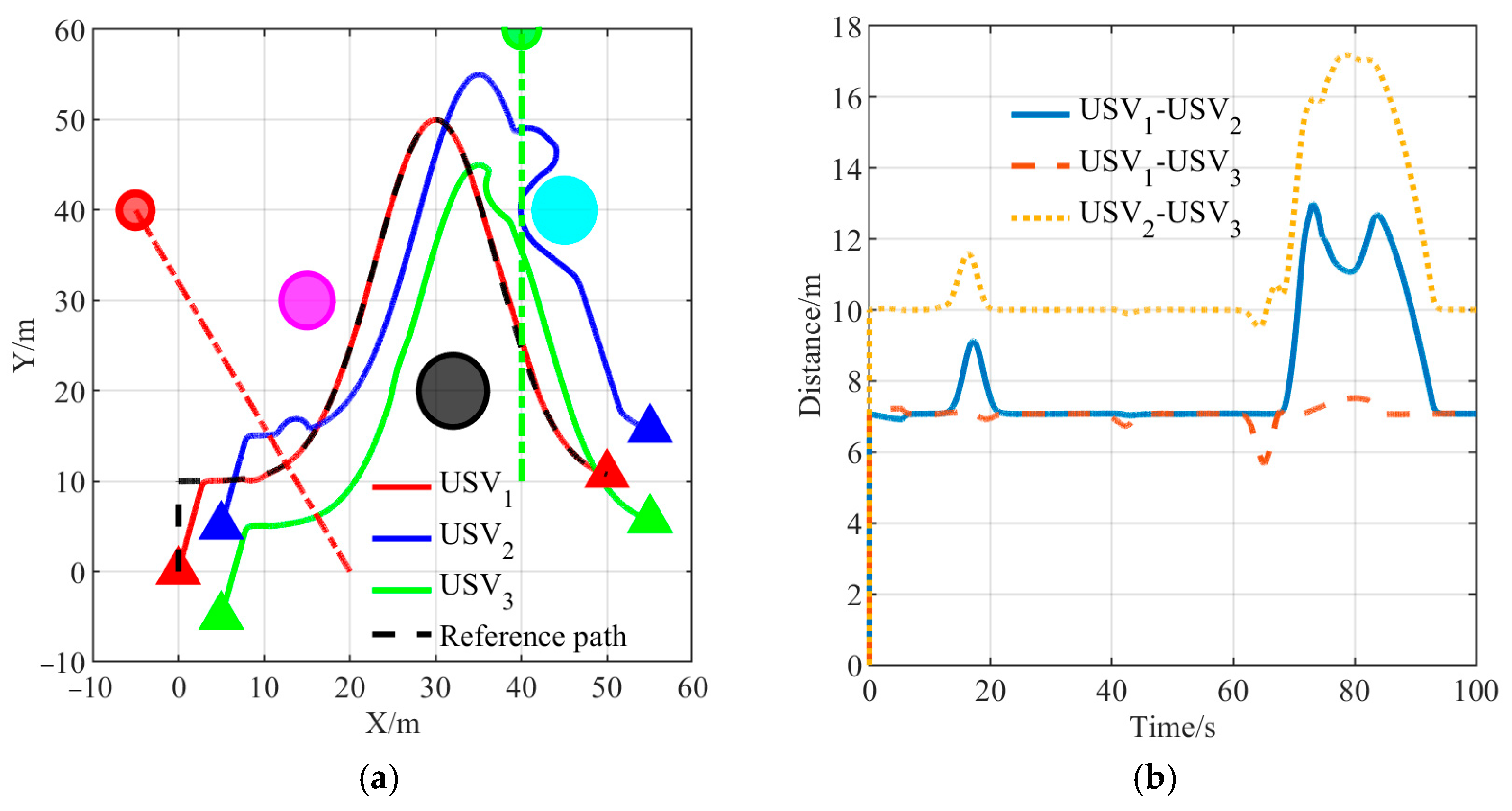
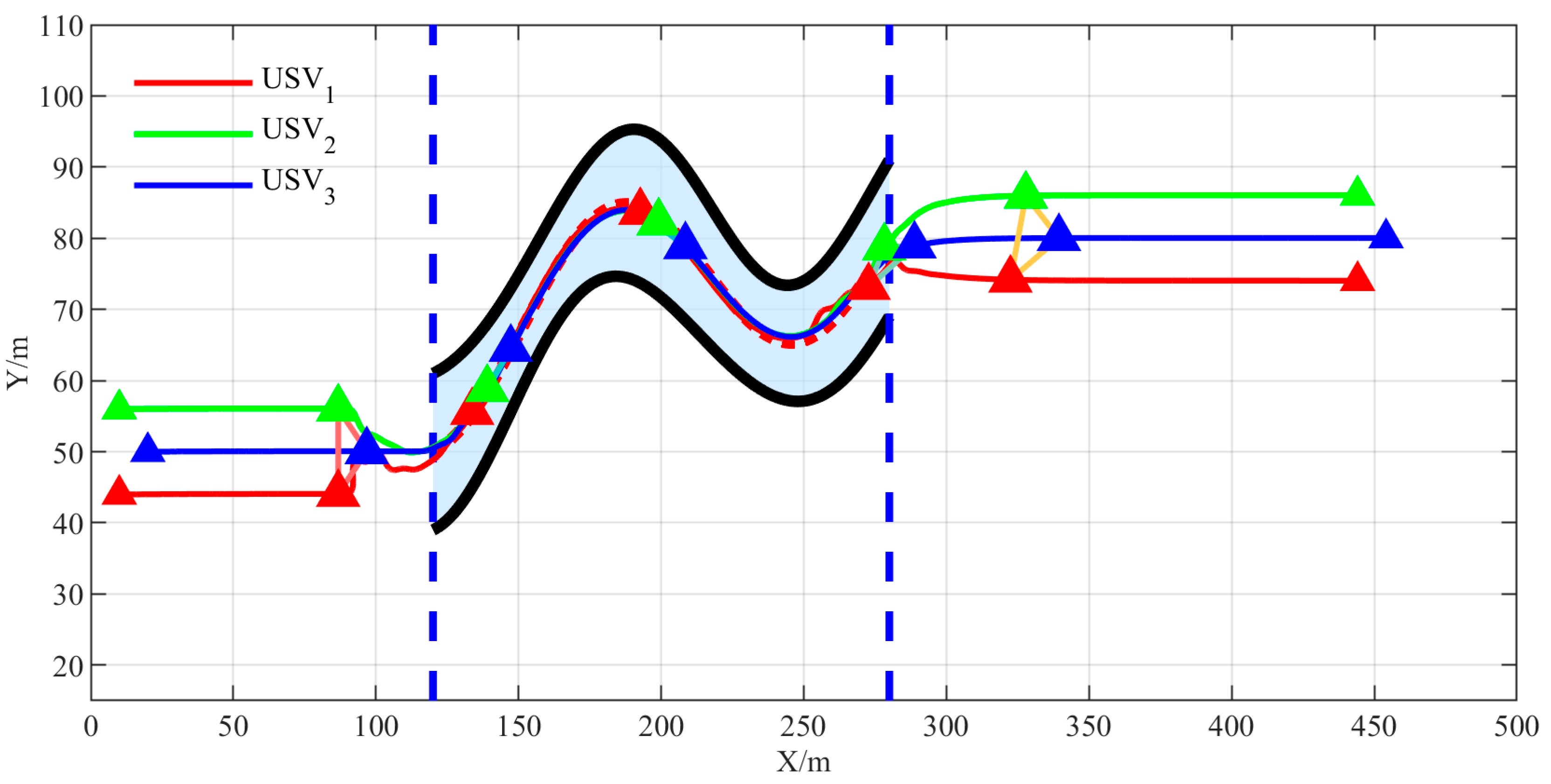
4.1. Avoiding Static and Dynamic Obstacles

Consider a formation system composed of three unmanned vehicles, initially positioned at $\left(0,0\right)$, $\left(5,5\right)$, and $\left(5,-5\right)$. The vehicles form an isosceles triangle, with each side having a length of $\left(5\sqrt{2},5\sqrt{2},10\right)$. Ocean disturbances are modeled using a first-order Gaussian–Markov process, denoted by ${\dot{\tau }}_{iw}^k+{\mu }_{iw}^k{\tau }_{iw}^k=w_i^k,{\mu }_{iw}^k>0,k=u,\mathbf{v},r$, where $w_i^k$ represents white noise. The time constant is set to ${\mu }_{iw}^k=0.5$, and the mean white noise $w_i^k$ is zero, with a variance of 0.5. The sampling period of the model predictive controller is $T_s=0.1$, the prediction horizon is $N_p=20$, and the control horizon is $N_c=5$. Reference paths are generated offline using Gaussian functions. Based on the aforementioned simulation parameters and disturbance settings, the obstacle avoidance performance is determined.

As demonstrated in Figure 4, the multi-USV system, based on the hybrid algorithm proposed in this paper, effectively avoids both dynamic and static obstacles while ensuring that no collisions occur between the vehicles during operation. Additionally, the proposed algorithm enables the formation to effectively track the predefined reference path and avoid obstacles in a reasonable manner.

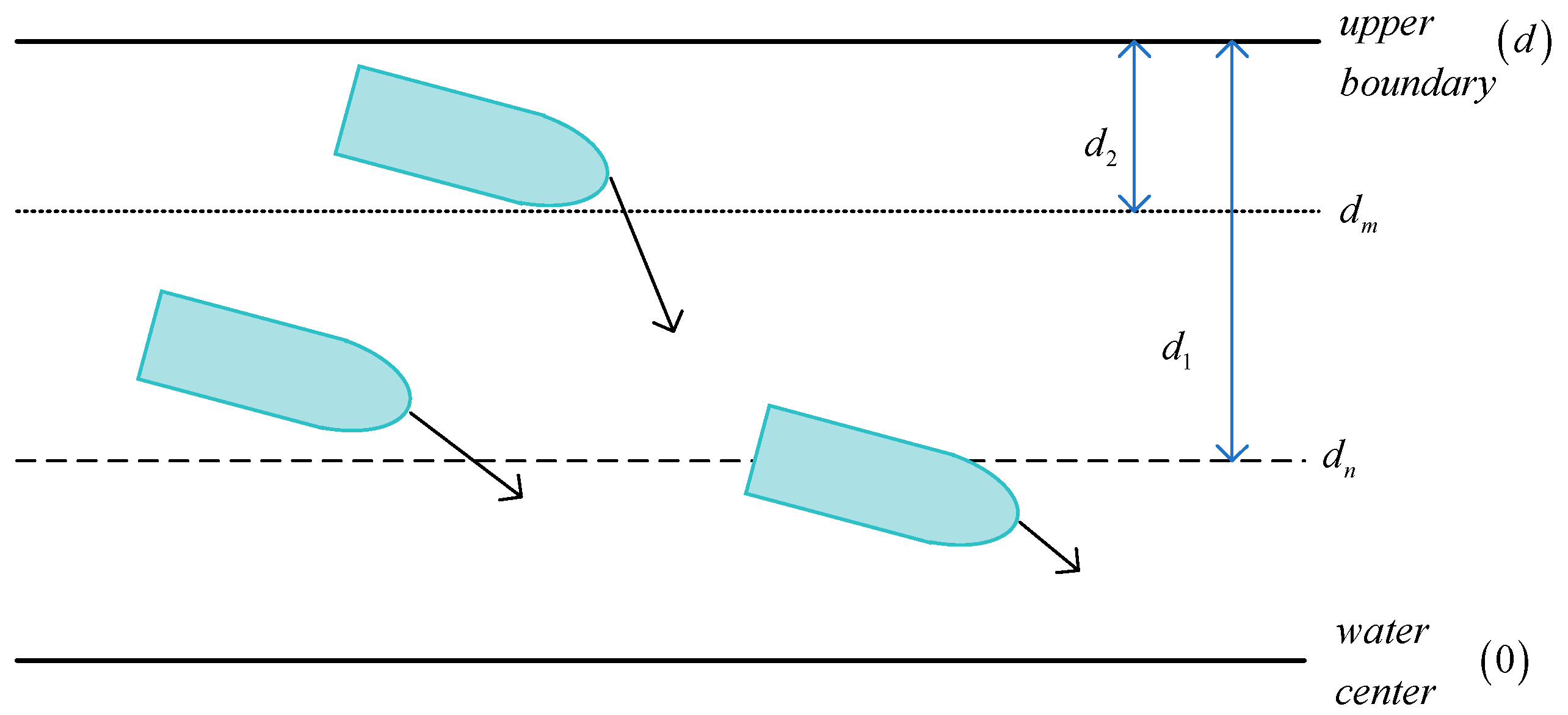
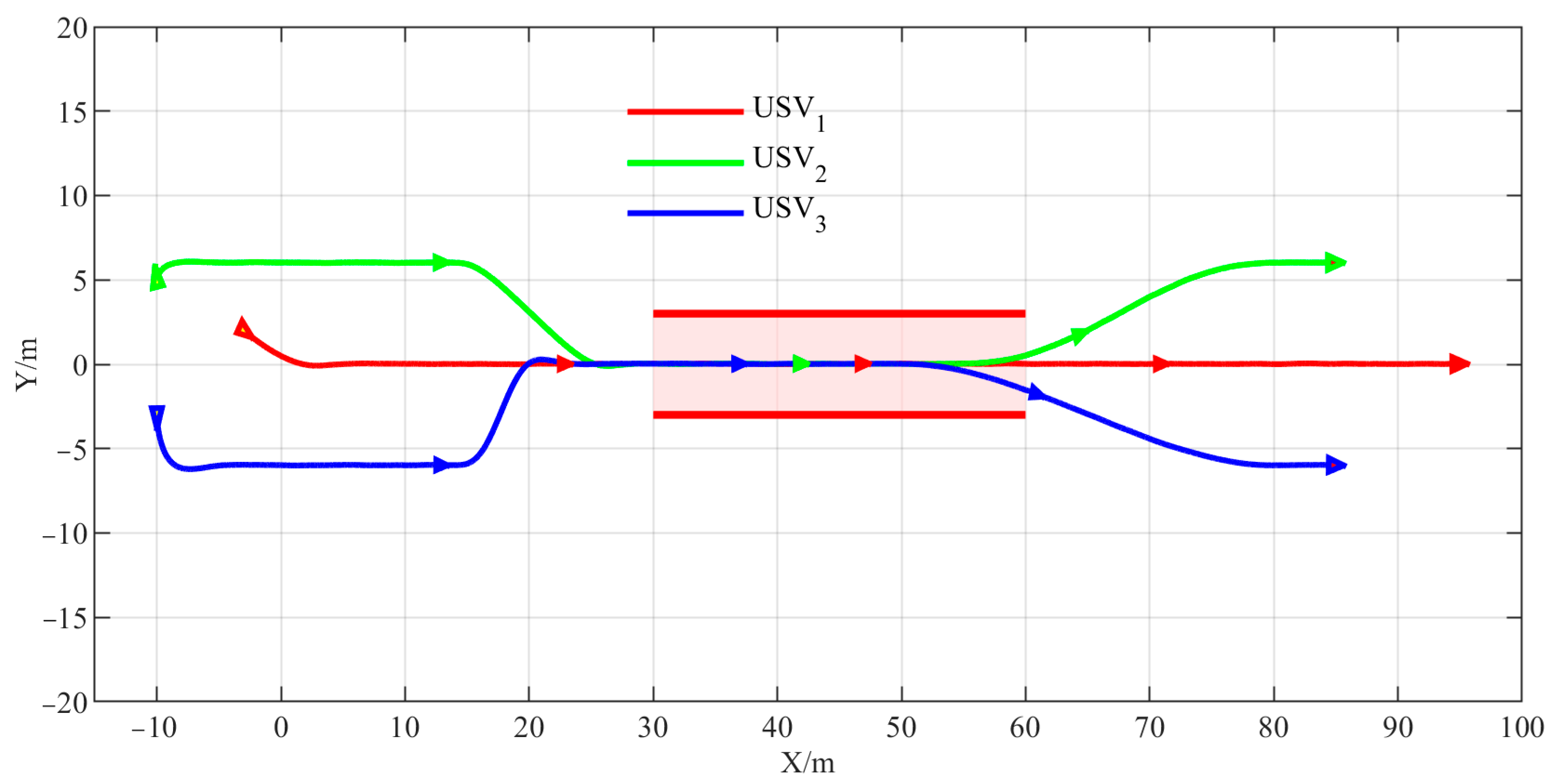
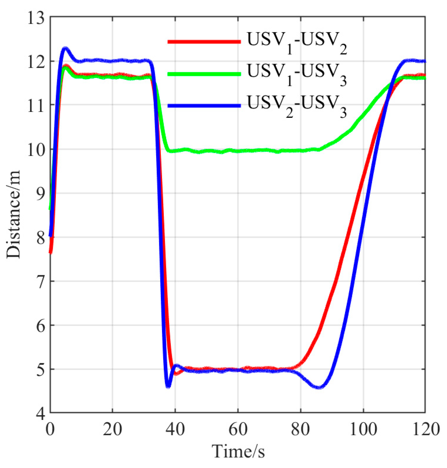
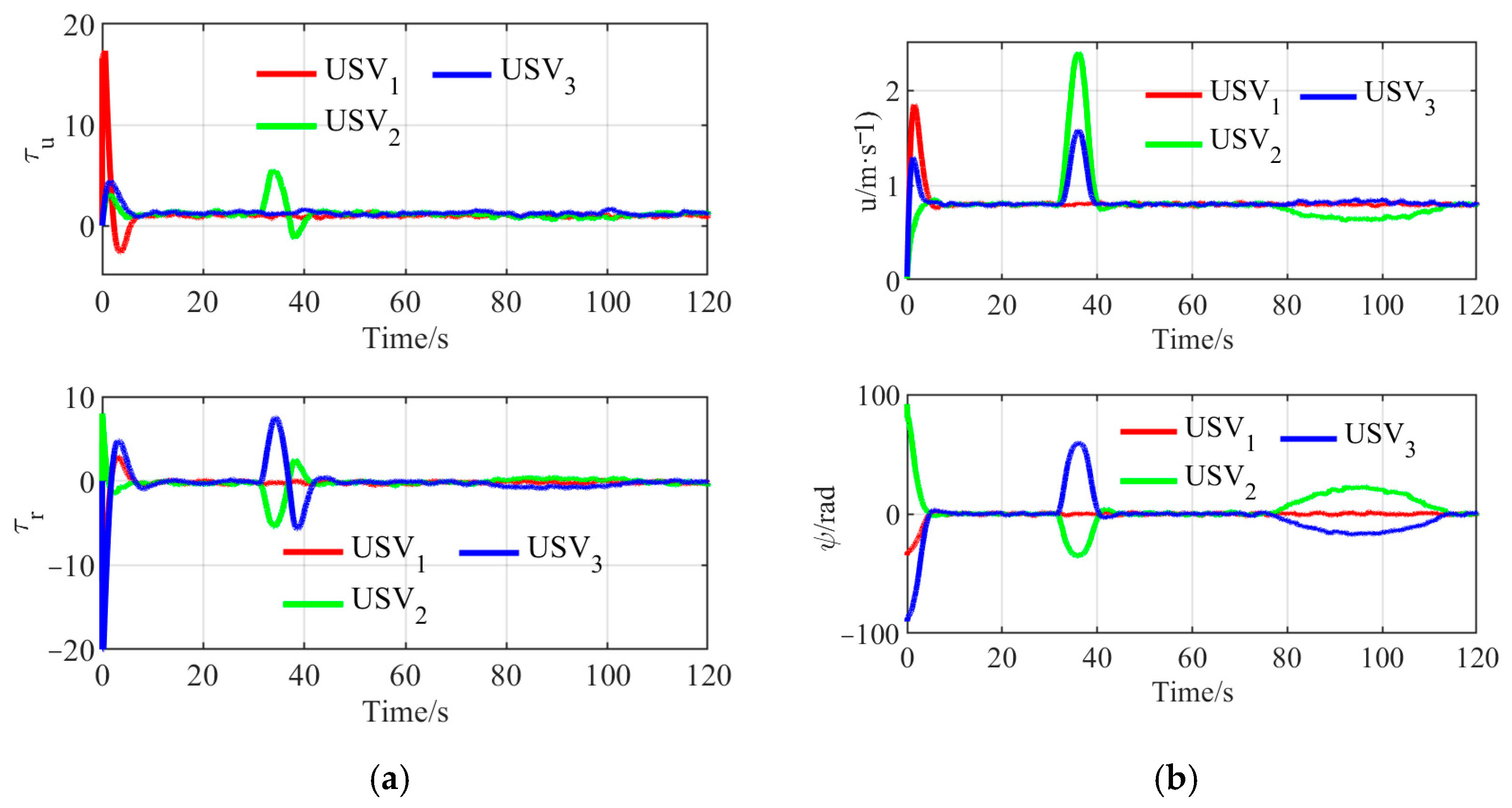
4.2. Navigating Through Narrow Waterways

During mission execution, the multi-USV formation frequently encounters narrow waterways or areas dense with obstacles, hindering its ability to maintain the original formation. Consequently, flexible formation adjustments and real-time obstacle avoidance are necessary to ensure safe passage. The initial positions of the formation members are (−3, 2), (−10, 5), and (−10, −3), arranged in a triangular formation with a side length of $\left(2\sqrt{34},2\sqrt{34},12\right)$, as defined by the virtual structure. A narrow area with a width of 6 is also established, as shown in Figure 5.

Figure 5 presents an overhead view of the USV formation navigating through a narrow waterway. As shown in Figure 5, Figure 6 and Figure 7, the formation moves smoothly through the narrow passage, following a continuous and stable trajectory. During the formation phase, the positions and headings of each USV are initially randomized. Once the formation is established, it maintains its structure throughout the movement. Upon encountering a narrow waterway, the formation transitions to a single column to pass through it and promptly returns to its original formation after clearing the passage, ultimately reaching the target point. Additionally, no collisions occur between the USVs during movement.

To further evaluate the algorithm’s applicability, we examined obstacle avoidance and formation behavior in an S-shaped narrow waterway. The formation is configured as a triangle, with initial positions at (10, 56), (10, 44), and (20, 50). The simulation results are depicted in Figure 8 and Figure 9.

The simulation results demonstrate that the proposed algorithm allows the vehicles to successfully navigate through the S-shaped narrow waterway by adapting their formation, swiftly restoring the original formation after they pass through. This validates the applicability and robustness of the proposed algorithm.

5. Conclusions

This paper addresses the control challenges faced by unmanned vehicle fleets in complex marine environments and proposes an integrated control strategy that combines an enhanced artificial potential field method with model predictive control. Through theoretical analysis and simulation, the effectiveness and practicality of the proposed method are validated. The improved artificial potential field method overcomes the inherent limitations of traditional potential field approaches. Specifically, the saturated attractive potential field eliminates oscillations near the target, while the partitioned repulsive potential field ensures that the fleet can safely navigate narrow waterways, offering a novel solution for path planning in constrained environments. The introduction of the extended state observer significantly improves the system’s robustness against disturbances, enabling accurate estimation of unknown dynamics and external environmental perturbations and providing reliable state information for subsequent controller design. The model predictive controller excels in managing system constraints, optimizing trajectory tracking and obstacle avoidance by incorporating potential field data into the objective function. The rolling-horizon strategy guarantees real-time control, effectively meeting the obstacle avoidance requirements imposed on the fleet. Stability analysis based on Lyapunov theory confirms the asymptotic stability of the multi-unmanned vehicle system, and the simulation results demonstrate the method’s effectiveness in scenarios such as static and dynamic obstacle avoidance and formation transitions in narrow waterways, highlighting its robustness and adaptability.

It is worth mentioning that the obstacles considered in this paper include reefs, shoals, locks, floating debris and so on, while vessel-related obstacles are not addressed. In future research, we will further explore how to incorporate COLREGs into the design framework, especially in multi-vessels collaboration and collision avoidance tasks in complex environments. Moreover, we will aim to use more formal and explicit collision risk indices (CRI) or similar quantitative risk metrics to monitor real-time risk levels and integrate them with COLREGs to enhance transparency and interpretability in high-stakes environments.

References

1. Sui, B.; Zhang, J.; Liu, Z. Prescribed-time formation tracking control for underactuated USVs with prescribed performance. J. Mar. Sci. Eng. 2025, 13, 480. [Google Scholar] [CrossRef]
2. Luo, Q.; Wang, H.; Li, N.; Zheng, W. Multi-unmanned surface vehicle model-free sliding mode predictive adaptive formation control and obstacle avoidance in complex marine environment via model-free extended state observer. Ocean Eng. 2024, 293, 116773. [Google Scholar] [CrossRef]
3. Zhang, S.; Zhang, Q.; Xu, L.; Xu, S.; Zhang, Y.; Hu, Y. Dynamic sliding mode formation control of unmanned surface vehicles under actuator failure. J. Mar. Sci. Eng. 2025, 13, 657. [Google Scholar] [CrossRef]
4. Yan, X.; Jiang, D.; Miao, R.; Li, Y. Formation control and obstacle avoidance algorithm of a multi-USV system based on virtual structure and artificial potential field. J. Mar. Sci. Eng. 2021, 9, 161. [Google Scholar] [CrossRef]
5. Liu, G.; Wen, N.; Long, F.; Zhang, R. A formation control and obstacle avoidance method for multiple unmanned surface vehicles. J. Mar. Sci. Eng. 2023, 11, 2346. [Google Scholar] [CrossRef]
6. Chang, Z.; Zong, G.; Wang, W.; Yue, M.; Zhao, X. Formation control and obstacle avoidance design for networked USV swarm with exogenous disturbance under intermittent communication. IEEE Trans. Netw. Sci. Eng. 2025, 12, 3234–3243. [Google Scholar] [CrossRef]
7. Lin, Y.; Du, L.; Yuen, K.F. Multiple unmanned surface vehicles pathfinding in dynamic environment. Appl. Soft Comput. 2025, 172, 112820. [Google Scholar] [CrossRef]
8. Luan, T.; Tan, Z.; You, B.; Sun, M.; Yao, H. Path planning of unmanned surface vehicle based on artificial potential field approach considering virtual target points. Trans. Inst. Meas. Control 2024, 46, 1190–1202. [Google Scholar] [CrossRef]
9. Li, W.; Zhang, X.; Wang, Y.; Xie, S. Comparison of linear and nonlinear model predictive control in path following of underactuated unmanned surface vehicles. J. Mar. Sci. Eng. 2024, 12, 575. [Google Scholar] [CrossRef]
10. Zheng, H.; Li, J.; Tian, Z.; Liu, C.; Wu, W. Hybrid physics-learning model based predictive control for trajectory tracking of unmanned surface vehicles. IEEE Trans. Intell. Transp. Syst. 2024, 25, 11522–11533. [Google Scholar] [CrossRef]
11. Jiang, L.; Wang, C.; Shang, X.; Zhang, Z. Two-step event-triggered data driven model predictive control for trajectory tracking of unmanned surface vessel under environmental disturbances. IEEE Trans. Autom. Sci. Eng. 2025, 22, 16801–16813. [Google Scholar] [CrossRef]
12. Morari, M.; Lee, J.H. Model predictive control: Past, present and future. Comput. Chem. Eng. 1999, 23, 667–682. [Google Scholar] [CrossRef]
13. Abdelaal, M.; Hahn, A. Predictive path following and collision avoidance of autonomous vessels in narrow channels. IFAC-PapersOnLine 2021, 54, 245–251. [Google Scholar] [CrossRef]
14. Wang, X.; Liu, J.; Peng, H.; Qie, X.; Zhao, X.; Lu, C. A simultaneous planning and control method integrating APF and MPC to solve autonomous navigation for USVs in unknown environments. J. Intell. Robot. Syst. 2022, 105, 36. [Google Scholar] [CrossRef]
15. Huang, Y.; Zhang, Z.; Sun, Q.; Li, Y. A formation motion control algorithm of unmanned surface vehicles based on DMPC and improved APF under unidirectional topologies. Unmanned Syst. Technol. 2022, 5, 1–11. [Google Scholar]
16. He, Z.; Chu, X.; Liu, C.; Wu, W. A novel model predictive artificial potential field based ship motion planning method considering COLREGs for complex encounter scenarios. ISA Trans. 2023, 134, 58–73. [Google Scholar] [CrossRef]
17. Li, H.; Wang, X.; Wu, T.; Ni, S. A COLREGs-Compliant ship collision avoidance decision-making support scheme based on improved APF and NMPC. J. Mar. Sci. Eng. 2023, 11, 1408. [Google Scholar] [CrossRef]
18. Ning, B.; Sun, Q.; Wang, S.; Fan, Y. Multi-unmanned surface vehicles formation based on DMPC and improved APF Method. In Proceedings of the 2023 IEEE 23rd International Conference on Communication Technology (ICCT), Wuxi, China, 20–22 October 2023; IEEE: New York, NY, USA, 2023; pp. 117–122. [Google Scholar]
19. Han, S.; Sun, J.; Ding, S.; Zhou, L. A potential field-based model predictive target following controller for underactuated unmanned surface vehicles. IEEE Trans. Veh. Technol. 2024, 73, 14510–14524. [Google Scholar] [CrossRef]
20. Menges, D.; Tengesdal, T.; Rasheed, A. Nonlinear model predictive control for enhanced navigation of autonomous surface vessels. IFAC-PapersOnLine 2024, 58, 296–302. [Google Scholar] [CrossRef]
21. Li, H.; Wang, X.; Soares, C.G.; Ni, S. A collision-avoidance decision-making scheme based on artificial potential fields and event-triggered control. Ocean Eng. 2024, 306, 118101. [Google Scholar] [CrossRef]
22. Li, W.; Wu, J.; Long, C. Formation control for unmanned surface vehicles based on integrative APF and MPC. In Proceedings of the 2022 IEEE International Conference on Robotics and Biomimetics (ROBIO), Xishuangbanna, China, 5–9 December 2022 2022; IEEE: New York, NY, USA, 2022; pp. 201–206. [Google Scholar]
23. Wang, L.; Pang, W.; Zhu, D. Event-triggered model predictive control algorithm for multi-AUV formation. Ordnance Ind. Autom. 2023, 42, 67–77. [Google Scholar]
24. Xue, Y.; Clelland, D.; Lee, B.; Han, D. Automatic simulation of ship navigation. Ocean. Eng. 2011, 38, 2290–2305. [Google Scholar] [CrossRef]
25. Wang, Z.; Im, N. Enhanced Artificial Potential Field for MASS’s Path Planning Navigation in Restricted Waterways. Appl. Ocean Res. 2024, 149, 104052. [Google Scholar] [CrossRef]
26. Do, K.D. Synchronization motion tracking control of multiple underactuated ships with collision avoidance. IEEE Trans. Ind. Electron. 2016, 63, 2976–2989. [Google Scholar] [CrossRef]
27. Zhen, Q.; Wan, L.; Li, Y.; Jiang, D. Formation control of a multi-AUVs system based on virtual structure and artificial potential field on SE(3). Ocean Eng. 2022, 253, 111148. [Google Scholar] [CrossRef]
28. Han, J. Extended state observer for a class of uncertain systems. Control Decis. 1995, 1, 85–88. [Google Scholar]
29. Gu, N.; Peng, Z.; Wang, D.; Shi, Y.; Wang, T. Antidisturbance coordinated path following control of robotic autonomous surface vehicles: Theory and experiment. IEEE/ASME Trans. Mechatron. 2019, 24, 2386–2396. [Google Scholar]
30. Liu, C.; Wang, D.; Zhang, Y.; Meng, X. Model predictive control for path following and roll stabilization of marine vessels based on neurodynamic optimization. Ocean Eng. 2020, 217, 107524. [Google Scholar] [CrossRef]
31. Kong, S.; Sun, J.; Qiu, C.; Wu, Z.; Yu, J. Extended state observer-based controller with model predictive governor for 3-D trajectory tracking of underactuated underwater vehicles. IEEE Trans. Ind. Inform. 2020, 17, 6114–6124. [Google Scholar] [CrossRef]
Figure 1. Unmanned surface vehicle coordinate system.
Jmse 13 01436 g001
Figure 2. A block diagram of the control scheme based on IAPF-ESO-MPC.
Jmse 13 01436 g002
Figure 3. Schematic diagram of zonal design for narrow waterways.
Jmse 13 01436 g003
Figure 4. Formation obstacle avoidance and tracking: (a) USV trajectory; (b) distances between USVs; (c) minimum distances between USVs and obstacles; (d) control inputs of USVs.
Jmse 13 01436 g004aJmse 13 01436 g004b
Figure 5. Performance in navigating narrow waterway.
Jmse 13 01436 g005
Figure 6. Distances between USVs.
Jmse 13 01436 g006
Figure 7. Status of USVs: (a) control input of USVs; (b) speed and heading of USVs.
Jmse 13 01436 g007
Figure 8. Performance in navigating an S-shaped narrow waterway.
Jmse 13 01436 g008
Figure 9. Control input of USVs.
Jmse 13 01436 g009
Disclaimer/Publisher’s Note: The statements, opinions and data contained in all publications are solely those of the individual author(s) and contributor(s) and not of MDPI and/or the editor(s). MDPI and/or the editor(s) disclaim responsibility for any injury to people or property resulting from any ideas, methods, instructions or products referred to in the content.