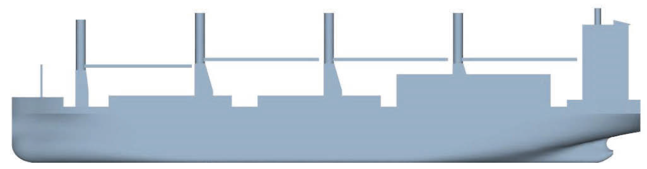
Figure 1.
Schematic diagram of the target ship.
Figure 1.
Schematic diagram of the target ship.
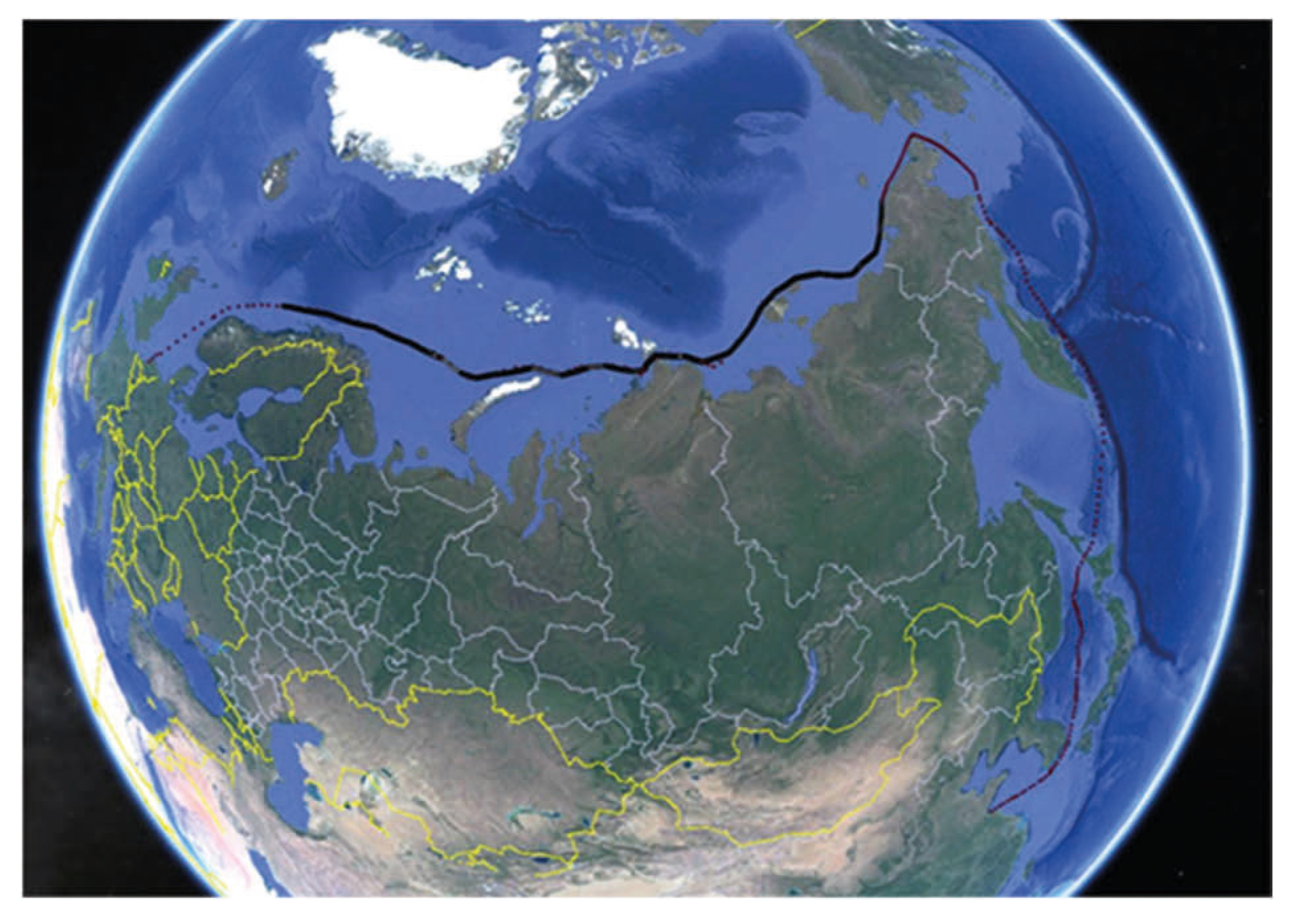
Figure 2.
Target ship trajectory.
Figure 2.
Target ship trajectory.
Figure 3.
Schematic diagram of wind data synthesis.
Figure 3.
Schematic diagram of wind data synthesis.
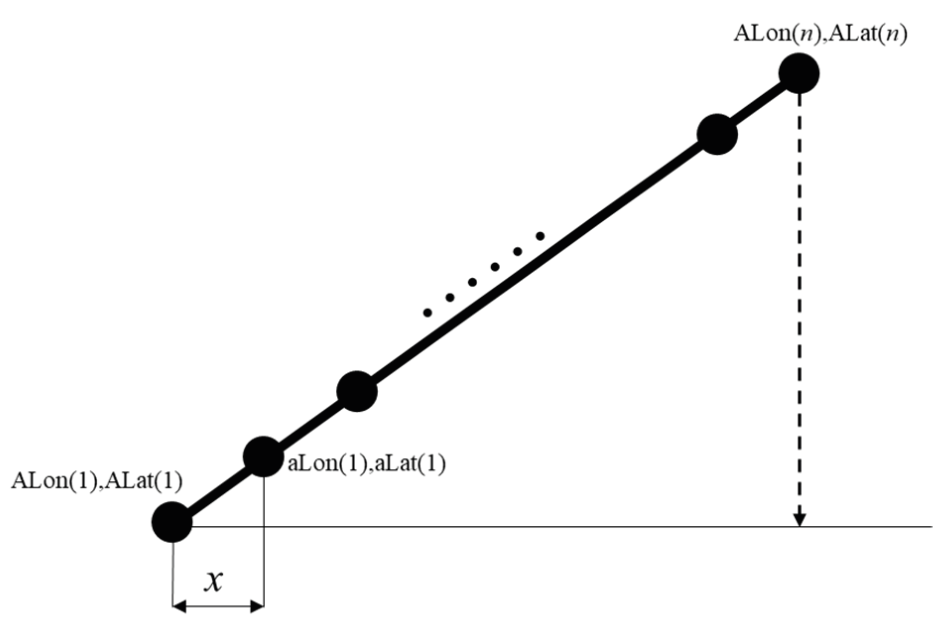
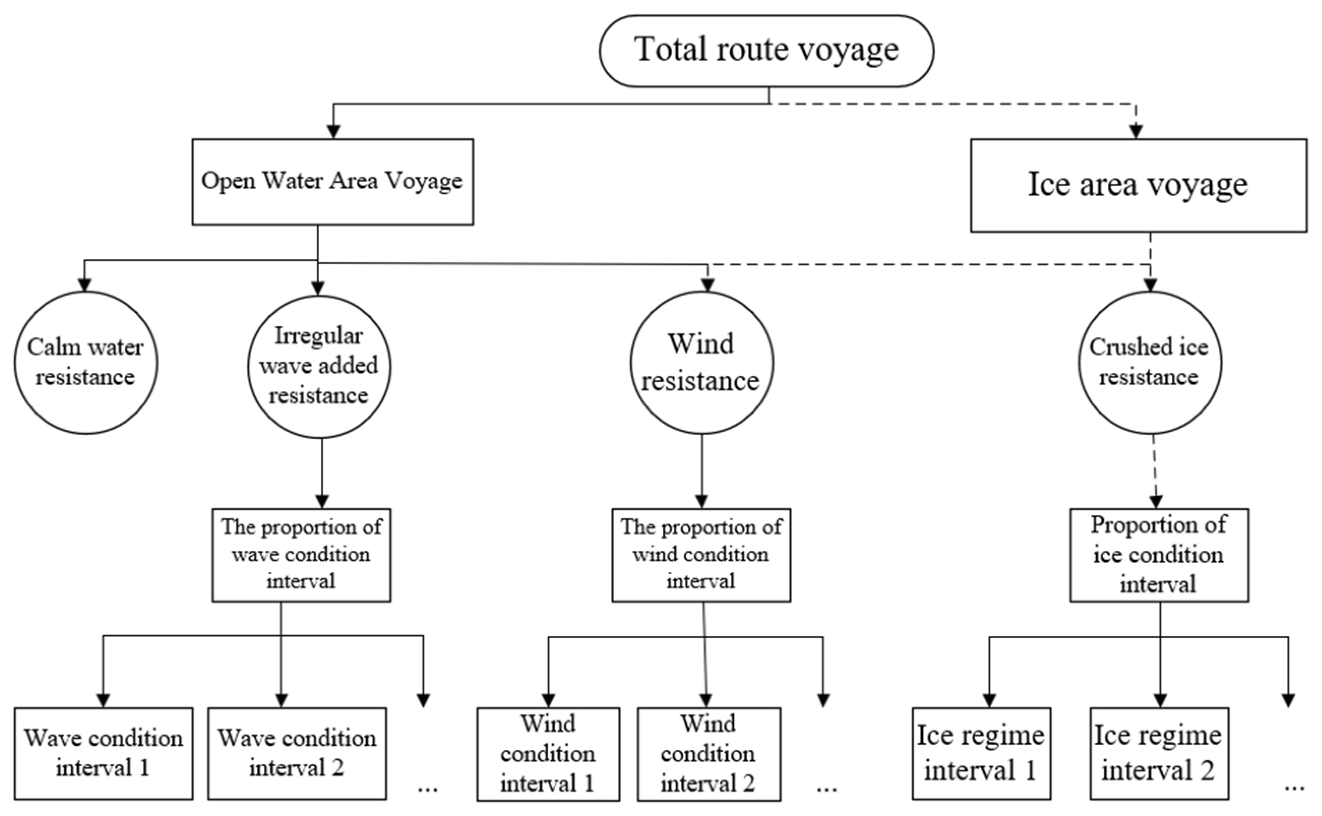
Figure 4.
Schematic diagram of fitting.
Figure 4.
Schematic diagram of fitting.
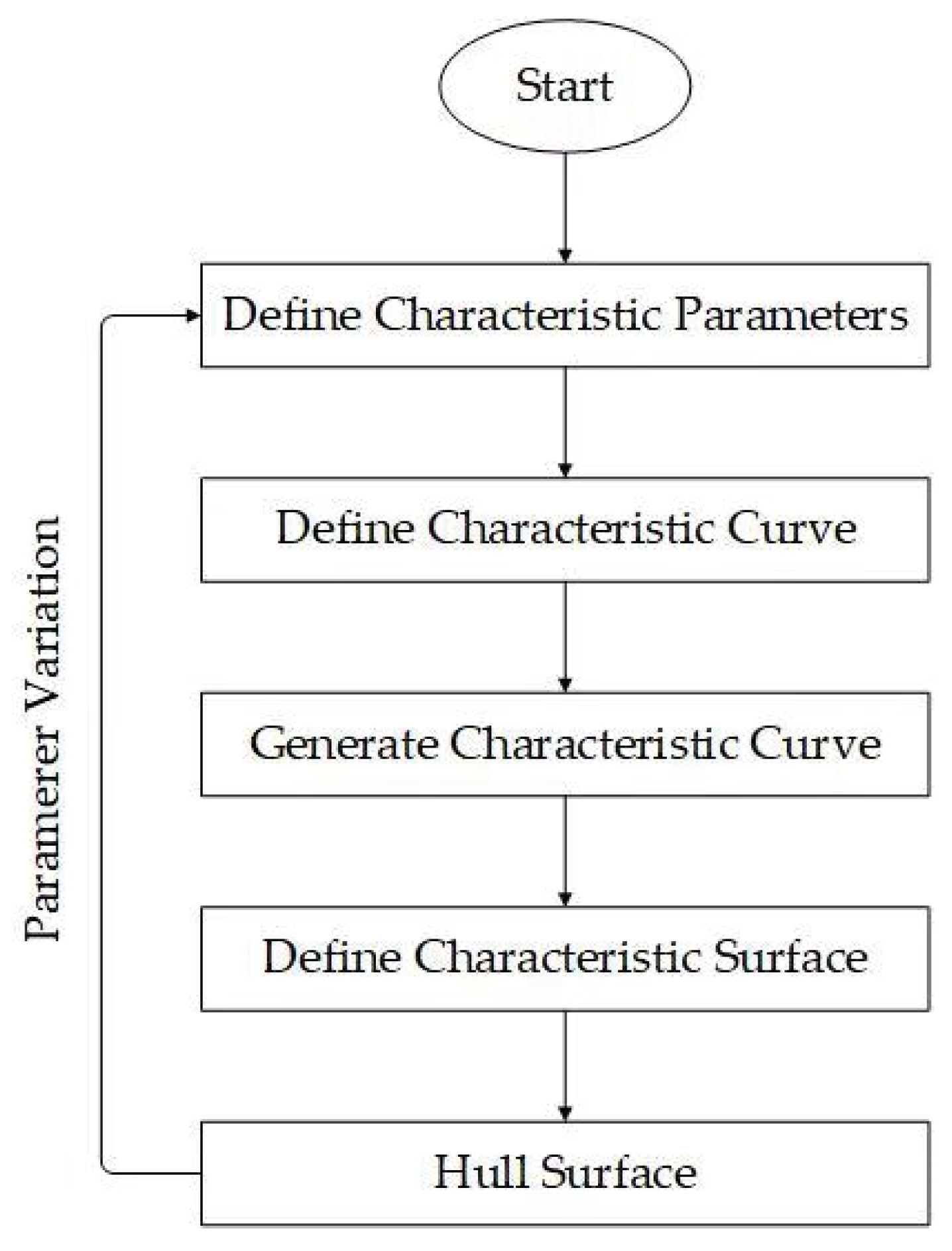
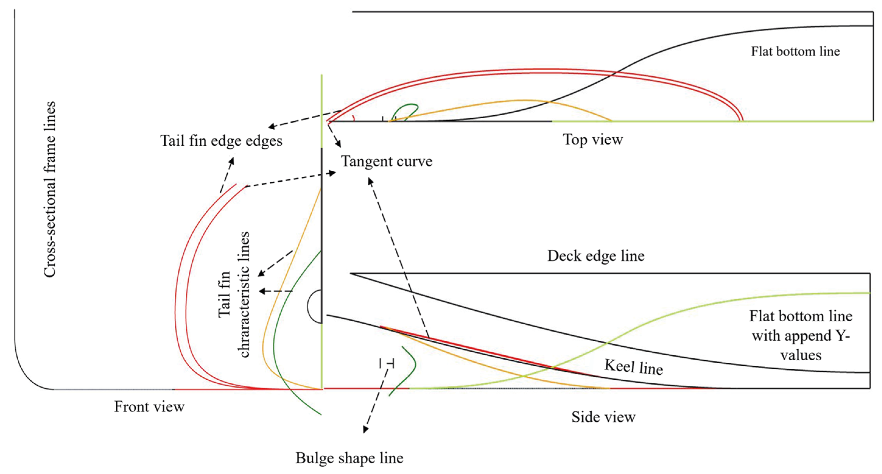
Figure 5.
Hull parametric modeling process.
Figure 5.
Hull parametric modeling process.
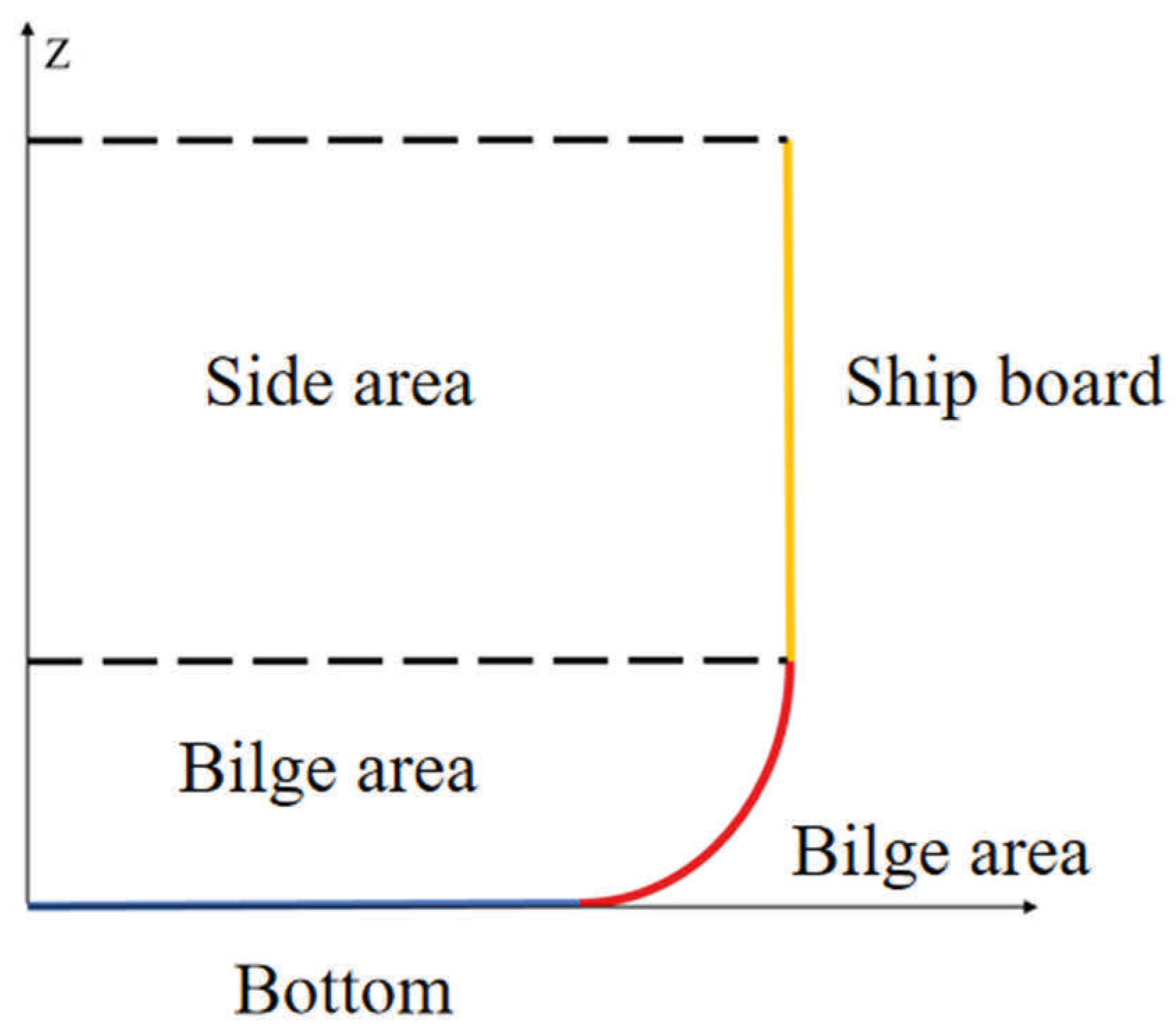
Figure 6.
Schematic diagram of the cross-sectional frame.
Figure 6.
Schematic diagram of the cross-sectional frame.
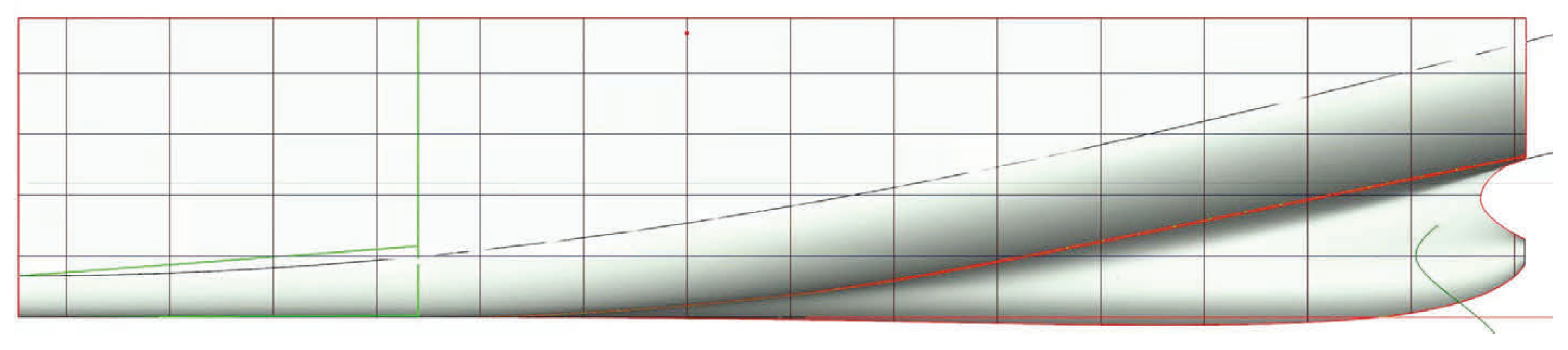
Figure 7.
Stern and skeg curve.
Figure 7.
Stern and skeg curve.
Figure 8.
Stern and skeg surface.
Figure 8.
Stern and skeg surface.
Figure 9.
Delta shift bow deformation control.
Figure 9.
Delta shift bow deformation control.
Figure 10.
Lackenby hull deformation control.
Figure 10.
Lackenby hull deformation control.
Figure 11.
Weight ratio analysis diagram.
Figure 11.
Weight ratio analysis diagram.
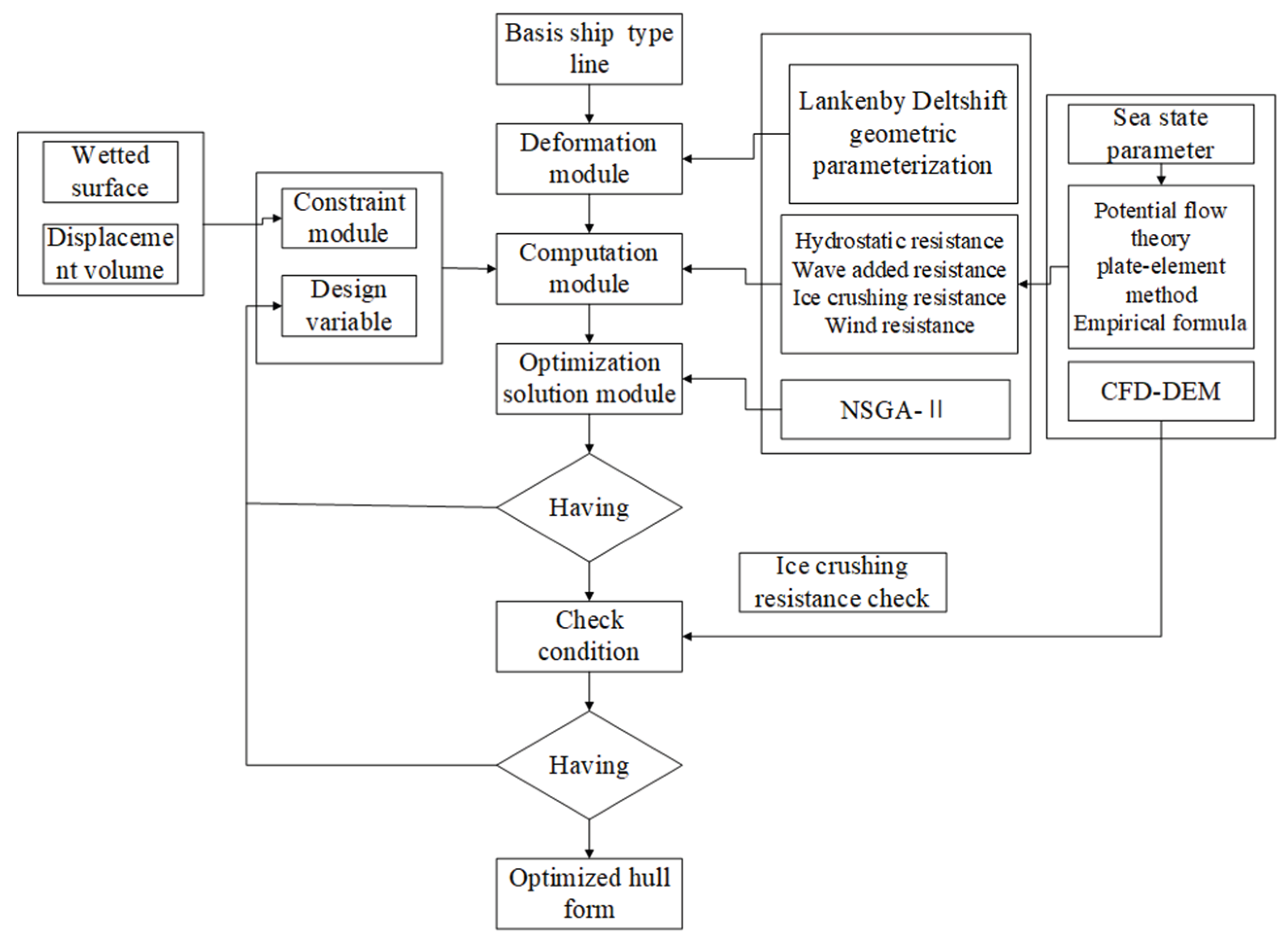
Figure 12.
Process of hull form optimization.
Figure 12.
Process of hull form optimization.
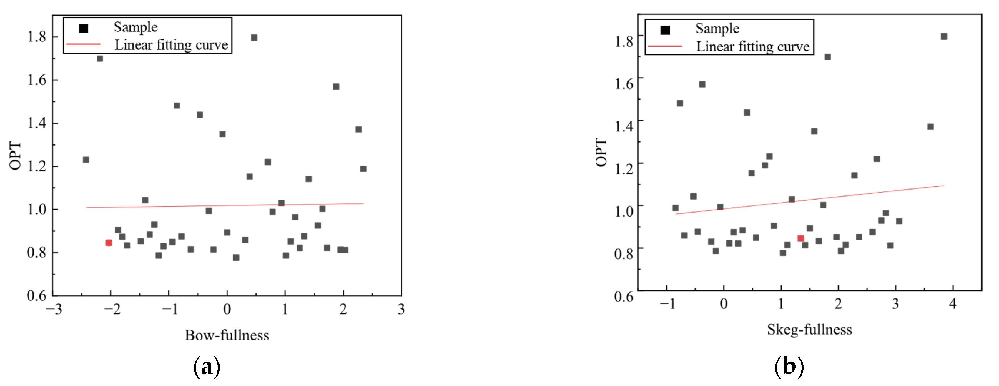
Figure 13.
The Sobol solution set distribution. (a) Optimization objective and Bow-fullness sensitivity; (b) Optimization objective and Skeg-fullness sensitivity; (c) Optimization objective and △CP sensitivity; (d) Optimization objective and △Xcb sensitivity.
Figure 13.
The Sobol solution set distribution. (a) Optimization objective and Bow-fullness sensitivity; (b) Optimization objective and Skeg-fullness sensitivity; (c) Optimization objective and △CP sensitivity; (d) Optimization objective and △Xcb sensitivity.
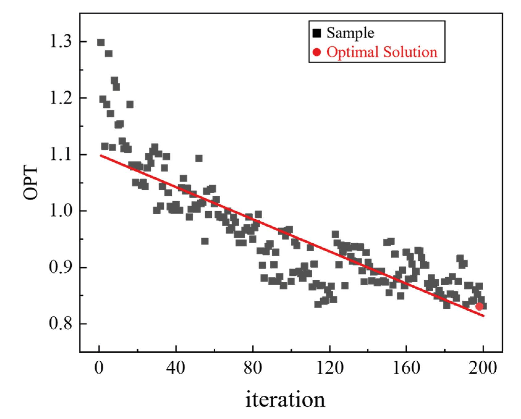
Figure 14.
Optimize the solution set.
Figure 14.
Optimize the solution set.
Figure 15.
Parameter correlation analysis. (a) Correlation between optimization objectives and Bow-fullness; (b) Correlation between optimization objectives and Skeg-fullness; (c) Correlation between optimization objectives and △CP; (d) Correlation between optimization objectives and △Xcb.
Figure 15.
Parameter correlation analysis. (a) Correlation between optimization objectives and Bow-fullness; (b) Correlation between optimization objectives and Skeg-fullness; (c) Correlation between optimization objectives and △CP; (d) Correlation between optimization objectives and △Xcb.
Figure 16.
Comparison of hull profiles (basis ship: black curve; optimized ship: red curve). (a) Waterline comparison; (b) Longitudinal section comparison.
Figure 16.
Comparison of hull profiles (basis ship: black curve; optimized ship: red curve). (a) Waterline comparison; (b) Longitudinal section comparison.
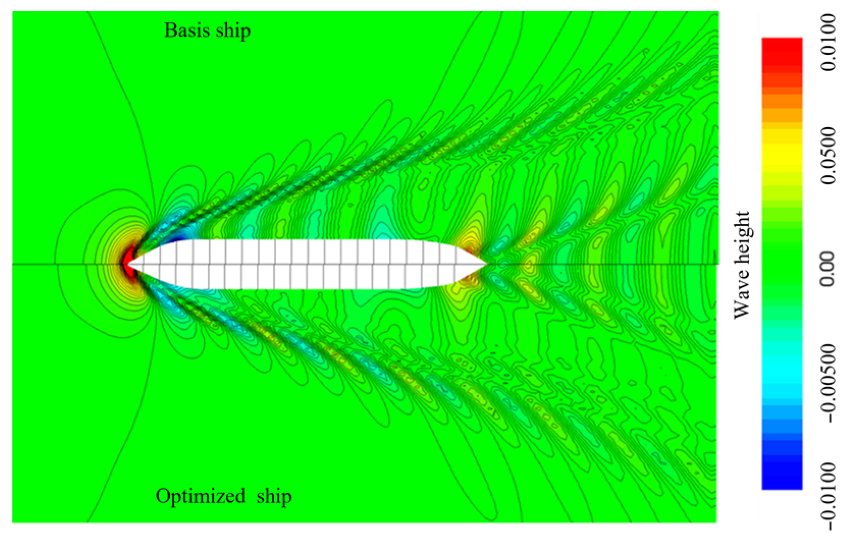
Figure 17.
Free surface comparison of basis and optimized ship.
Figure 17.
Free surface comparison of basis and optimized ship.
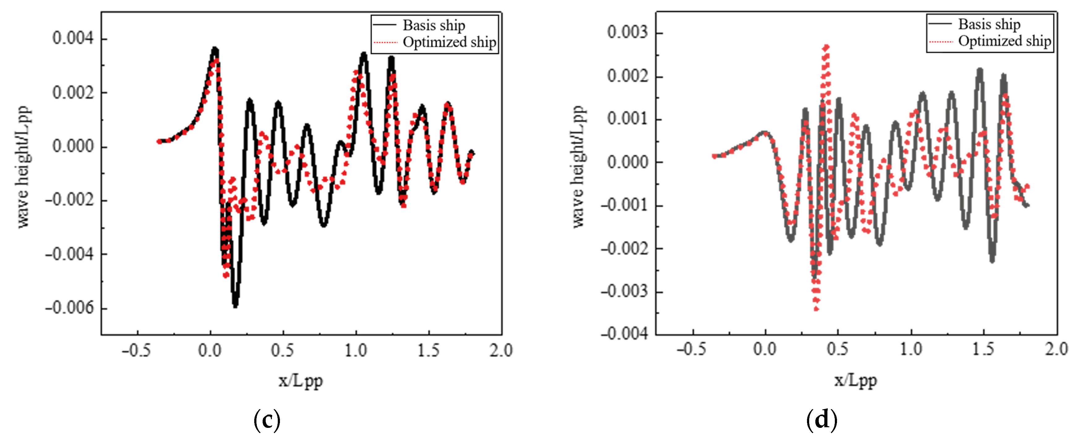
Figure 18.
Wave height of ships in different positions. (a) Ship traveling wave side wave height; (b) Free surface wave height; (c) Ship traveling wave height (y/Lpp = 0.1); (d) Ship traveling wave height (y/Lpp = 0.2).
Figure 18.
Wave height of ships in different positions. (a) Ship traveling wave side wave height; (b) Free surface wave height; (c) Ship traveling wave height (y/Lpp = 0.1); (d) Ship traveling wave height (y/Lpp = 0.2).
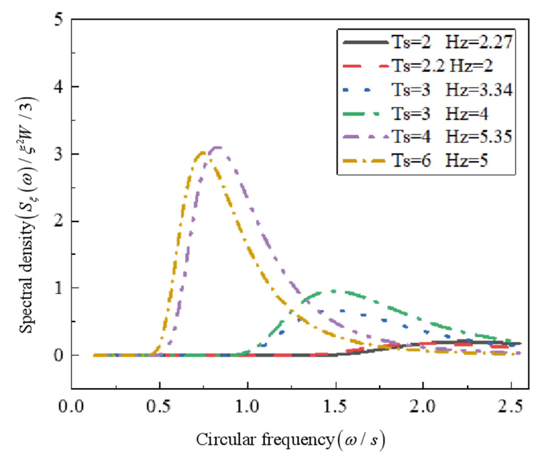
Figure 19.
ITTC two-parameter wave spectrum with different Hs and Tz.
Figure 19.
ITTC two-parameter wave spectrum with different Hs and Tz.
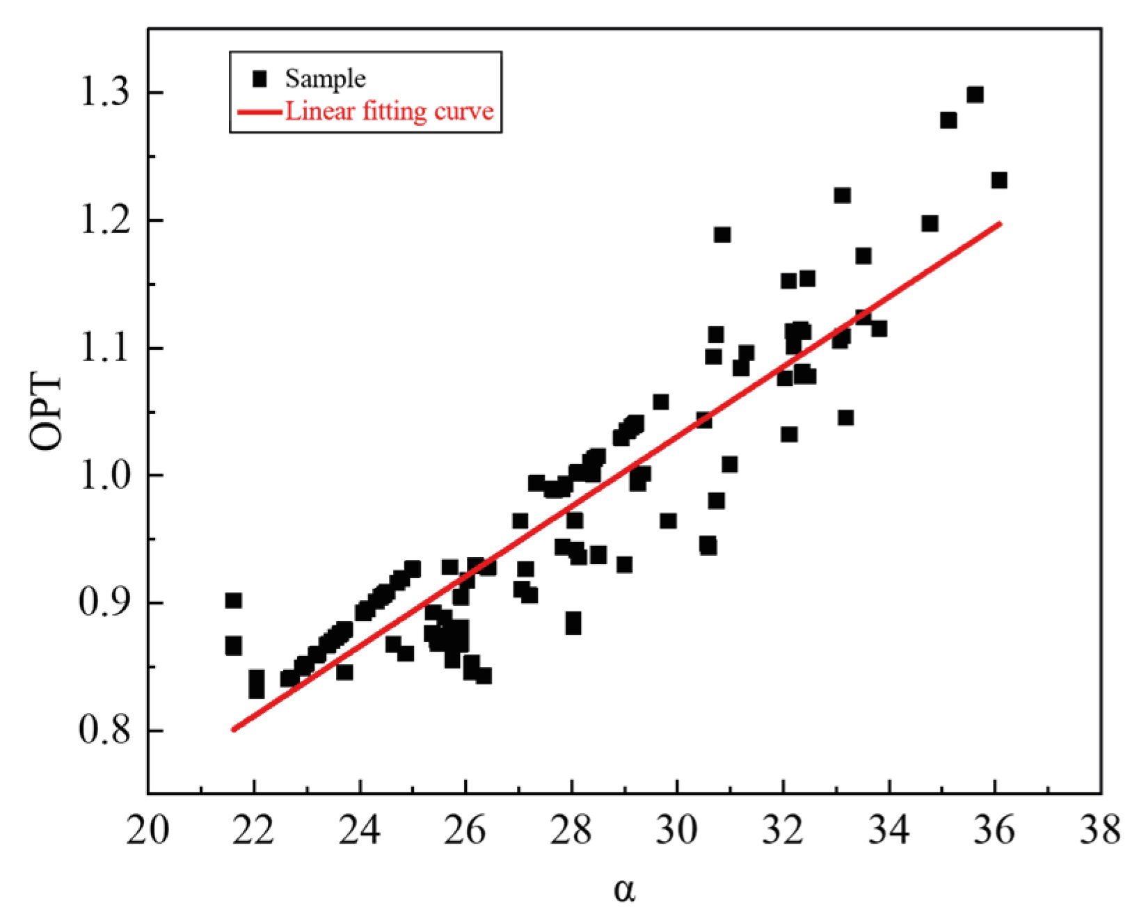
Figure 20.
Correlation between α and optimization goals.
Figure 20.
Correlation between α and optimization goals.
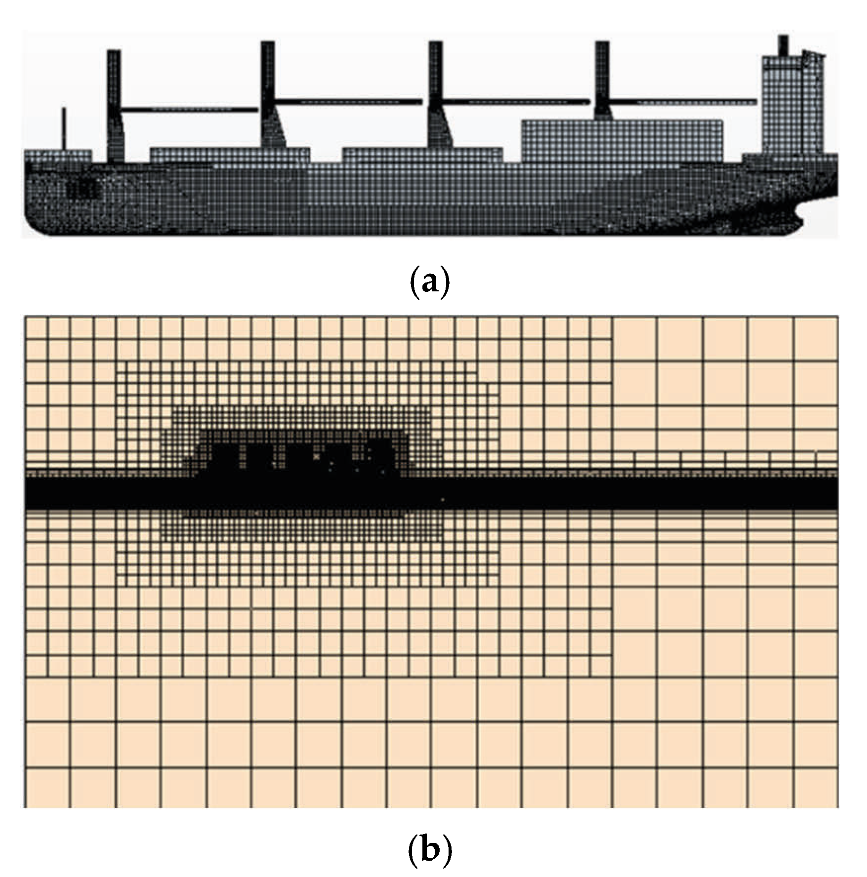
Figure 21.
Hull mesh and flow field longitudinal mesh. (a) Hull grid. (b) Grid of the longitudinal section of the flow field.
Figure 21.
Hull mesh and flow field longitudinal mesh. (a) Hull grid. (b) Grid of the longitudinal section of the flow field.
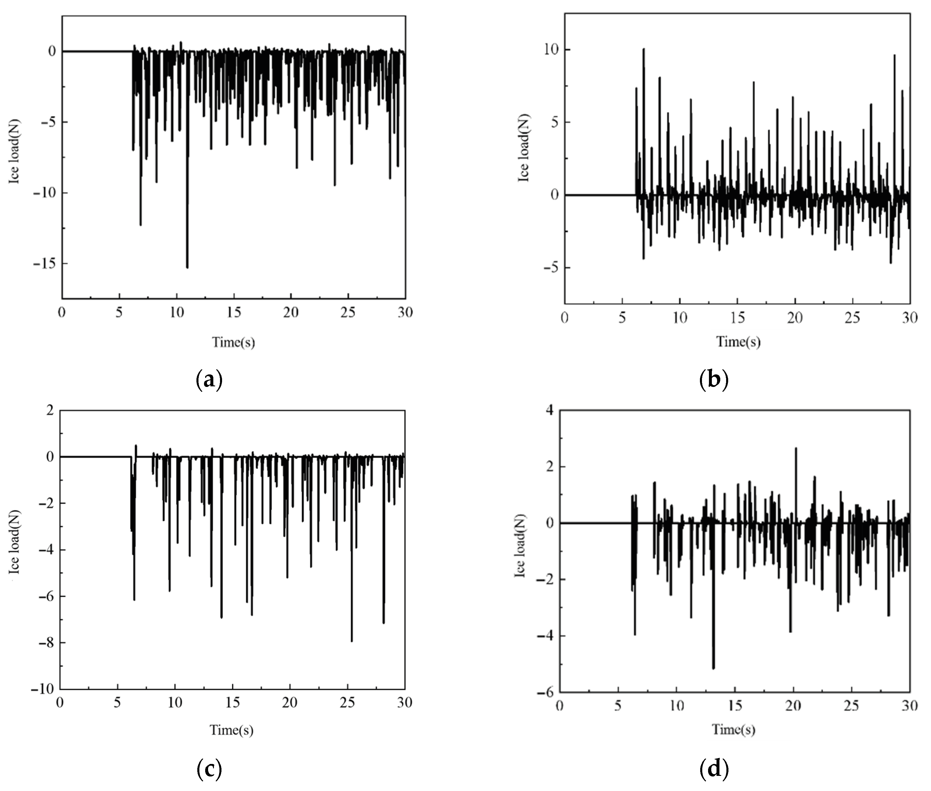
Figure 22.
Ice thickness 0.0215 m, density 40% of the ice load. (a) Longitudinal Force of basis ship in x-direction; (b) Longitudinal Force of basis ship in y-direction; (c) Longitudinal force in x-direction of the optimized ship. (d) Longitudinal force in y-direction of the optimized ship.
Figure 22.
Ice thickness 0.0215 m, density 40% of the ice load. (a) Longitudinal Force of basis ship in x-direction; (b) Longitudinal Force of basis ship in y-direction; (c) Longitudinal force in x-direction of the optimized ship. (d) Longitudinal force in y-direction of the optimized ship.
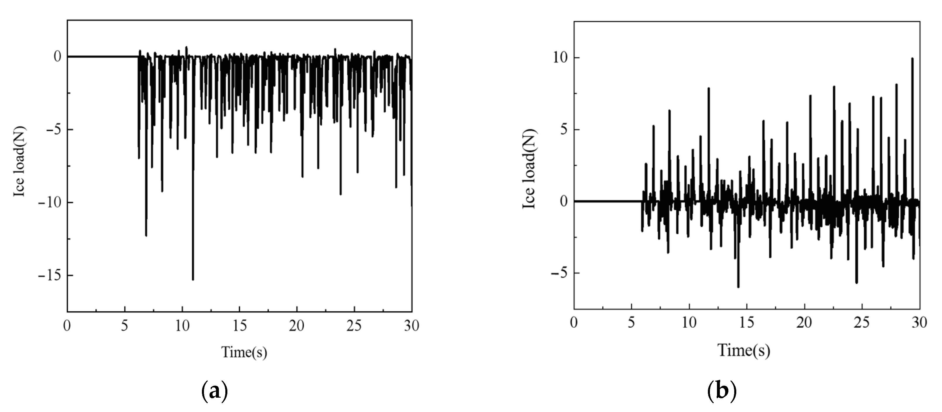
Figure 23.
Ice thickness 0.015 m, density 30% of the ice load. (a) Longitudinal Force of basis ship in x-direction; (b) Longitudinal Force of basis ship in y-direction; (c) Longitudinal force in x-direction of the optimized ship; (d) Longitudinal force in y-direction of the optimized ship.
Figure 23.
Ice thickness 0.015 m, density 30% of the ice load. (a) Longitudinal Force of basis ship in x-direction; (b) Longitudinal Force of basis ship in y-direction; (c) Longitudinal force in x-direction of the optimized ship; (d) Longitudinal force in y-direction of the optimized ship.
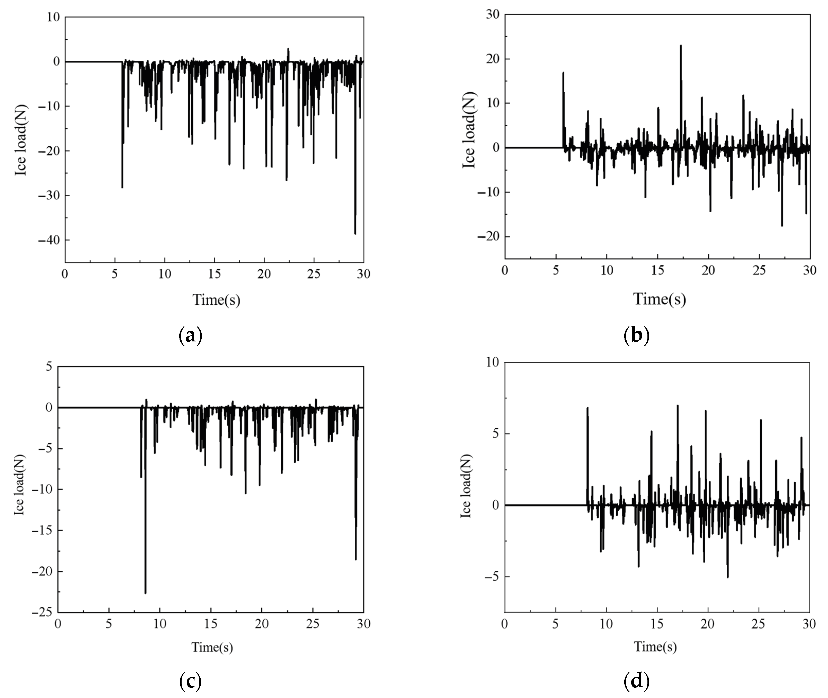
Figure 24.
Ice thickness 0.0107 m, density 50% of the ice load. (a) Longitudinal Force of basis ship in x-direction; (b) Longitudinal Force of basis ship in y-direction; (c) Longitudinal force in x-direction of the optimized ship; (d) Longitudinal force in y-direction of the optimized ship.
Figure 24.
Ice thickness 0.0107 m, density 50% of the ice load. (a) Longitudinal Force of basis ship in x-direction; (b) Longitudinal Force of basis ship in y-direction; (c) Longitudinal force in x-direction of the optimized ship; (d) Longitudinal force in y-direction of the optimized ship.
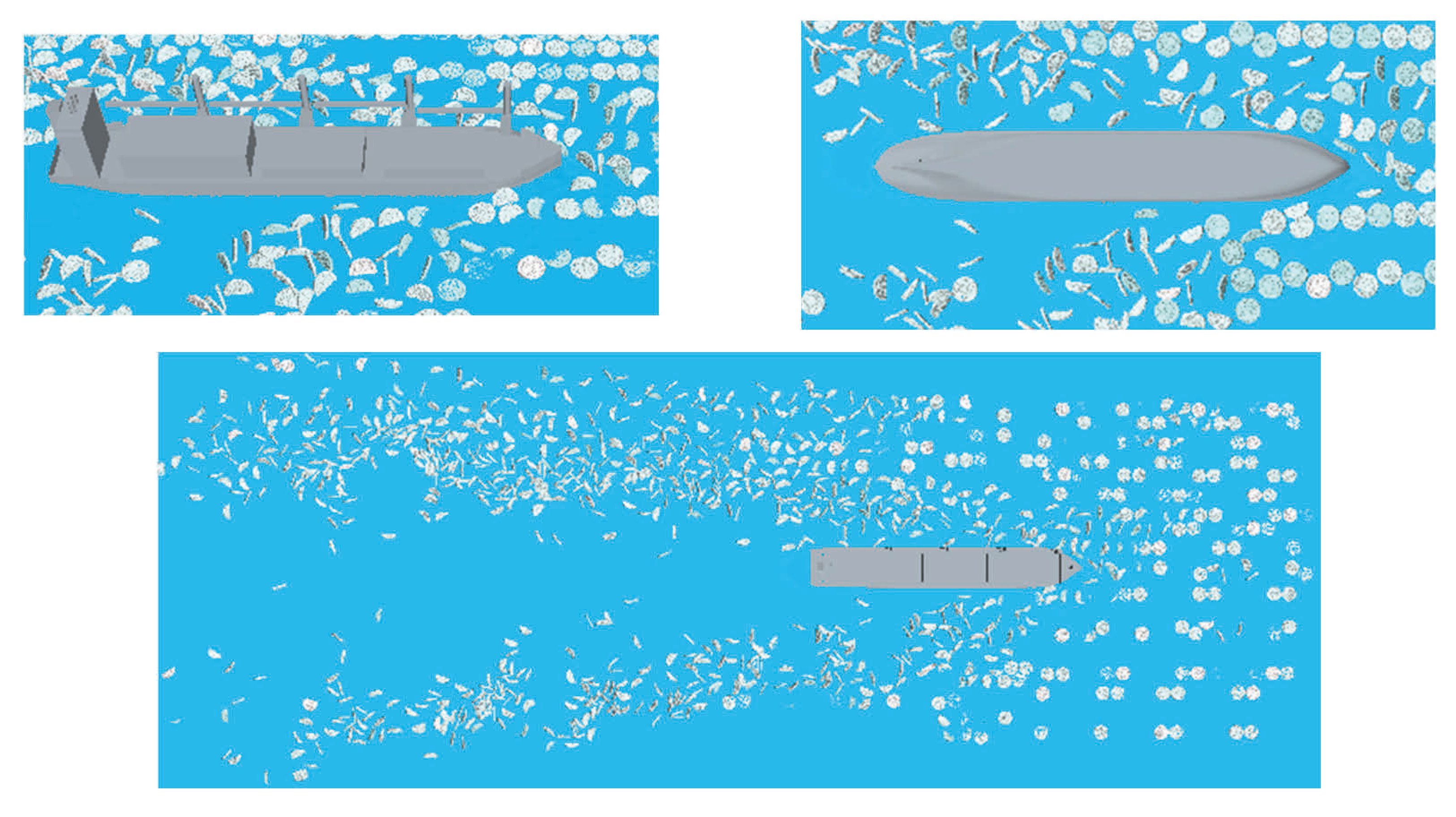
Figure 25.
The ice is 0.0107 m thick and 50% dense.
Figure 25.
The ice is 0.0107 m thick and 50% dense.
Figure 26.
Efficiency and Power Schematic.
Figure 26.
Efficiency and Power Schematic.
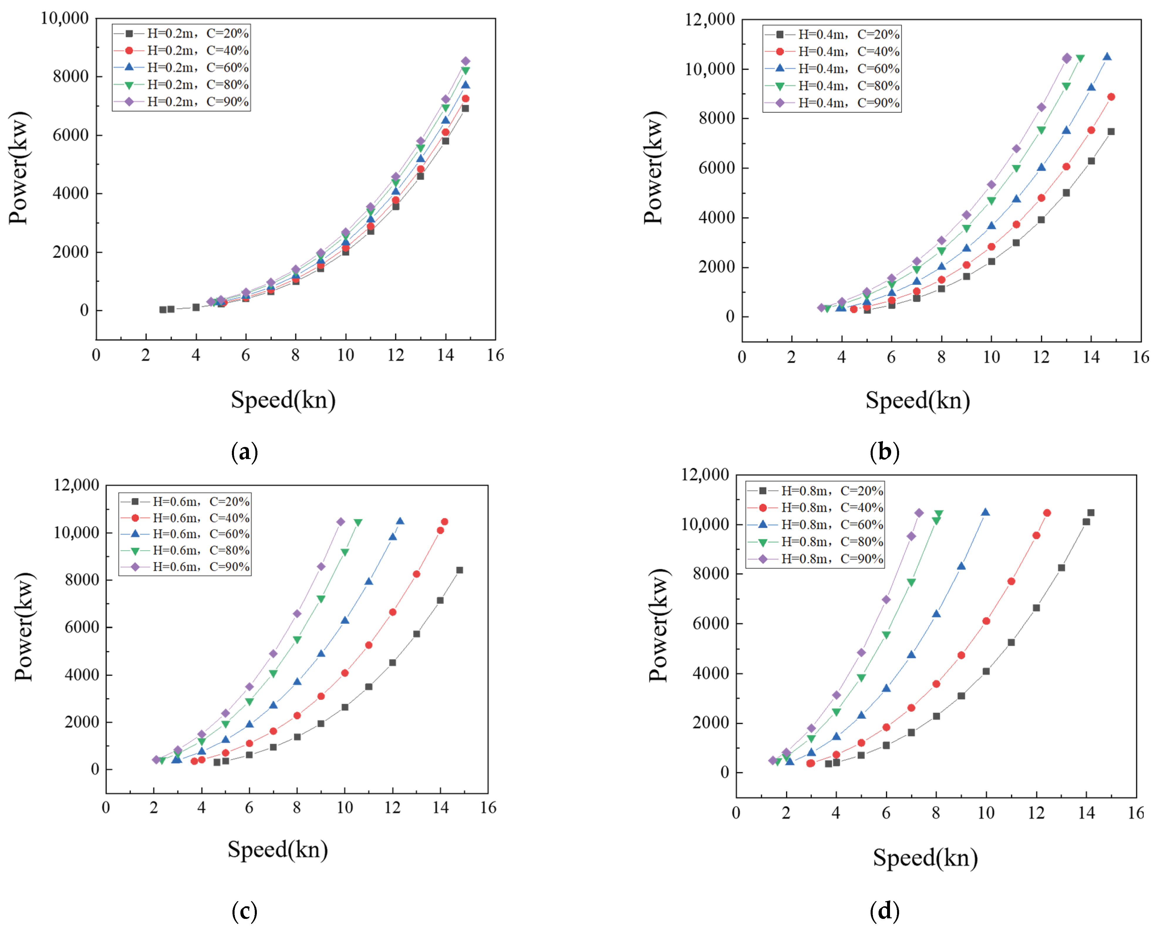
Figure 27.
Energy efficiency power under different ice. (a) Ice thickness 0.2 m; (b) Ice thickness 0.4 m; (c) Ice thickness 0.6 m; (d) Ice thickness 0.8 m.
Figure 27.
Energy efficiency power under different ice. (a) Ice thickness 0.2 m; (b) Ice thickness 0.4 m; (c) Ice thickness 0.6 m; (d) Ice thickness 0.8 m.
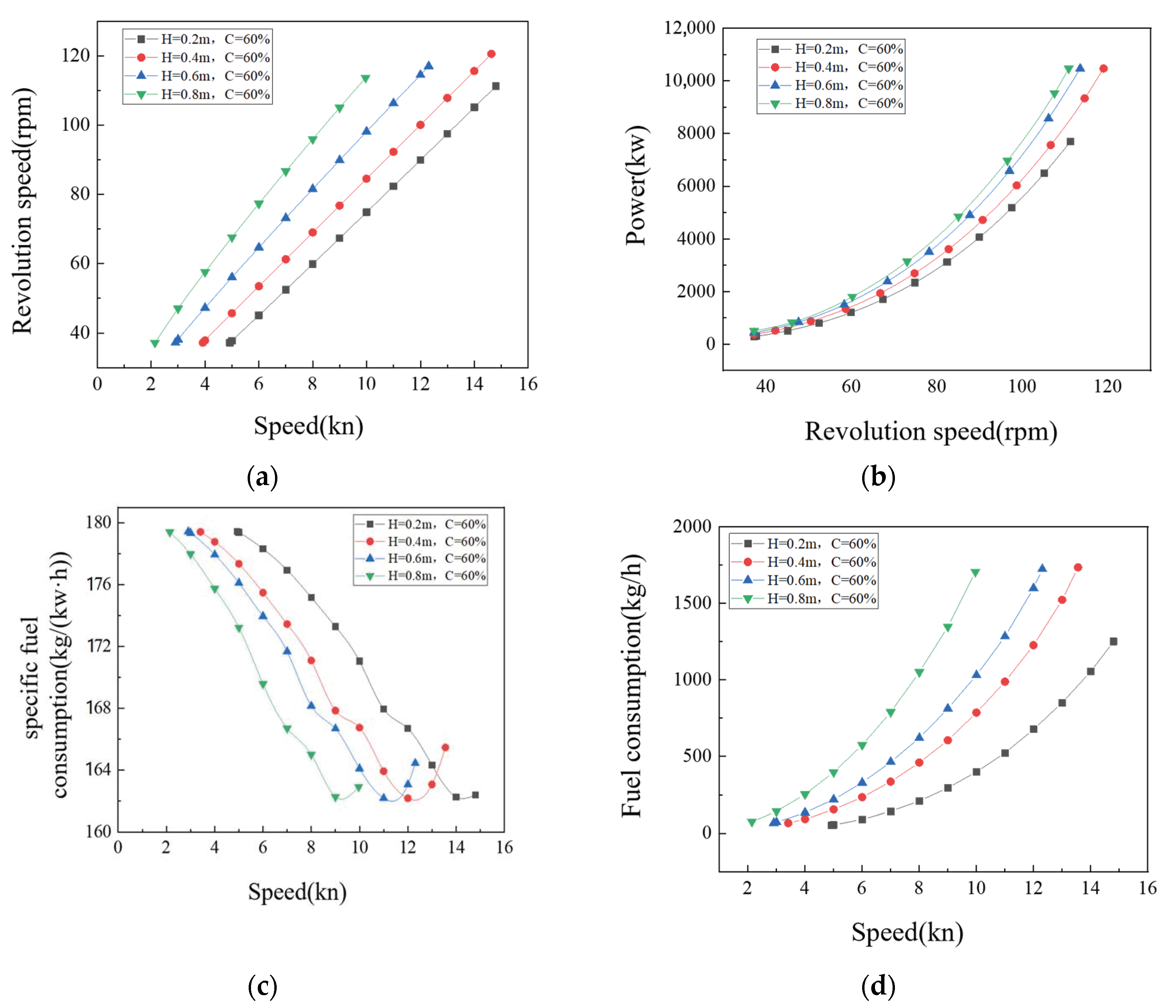
Figure 28.
Energy efficiency analysis for different ice thicknesses at 60% density. (a) Speed—Revolution speed. (b) Revolution speed—Power. (c) Speed—Specific fuel consumption. (d) Speed—Fuel consumption.
Figure 28.
Energy efficiency analysis for different ice thicknesses at 60% density. (a) Speed—Revolution speed. (b) Revolution speed—Power. (c) Speed—Specific fuel consumption. (d) Speed—Fuel consumption.
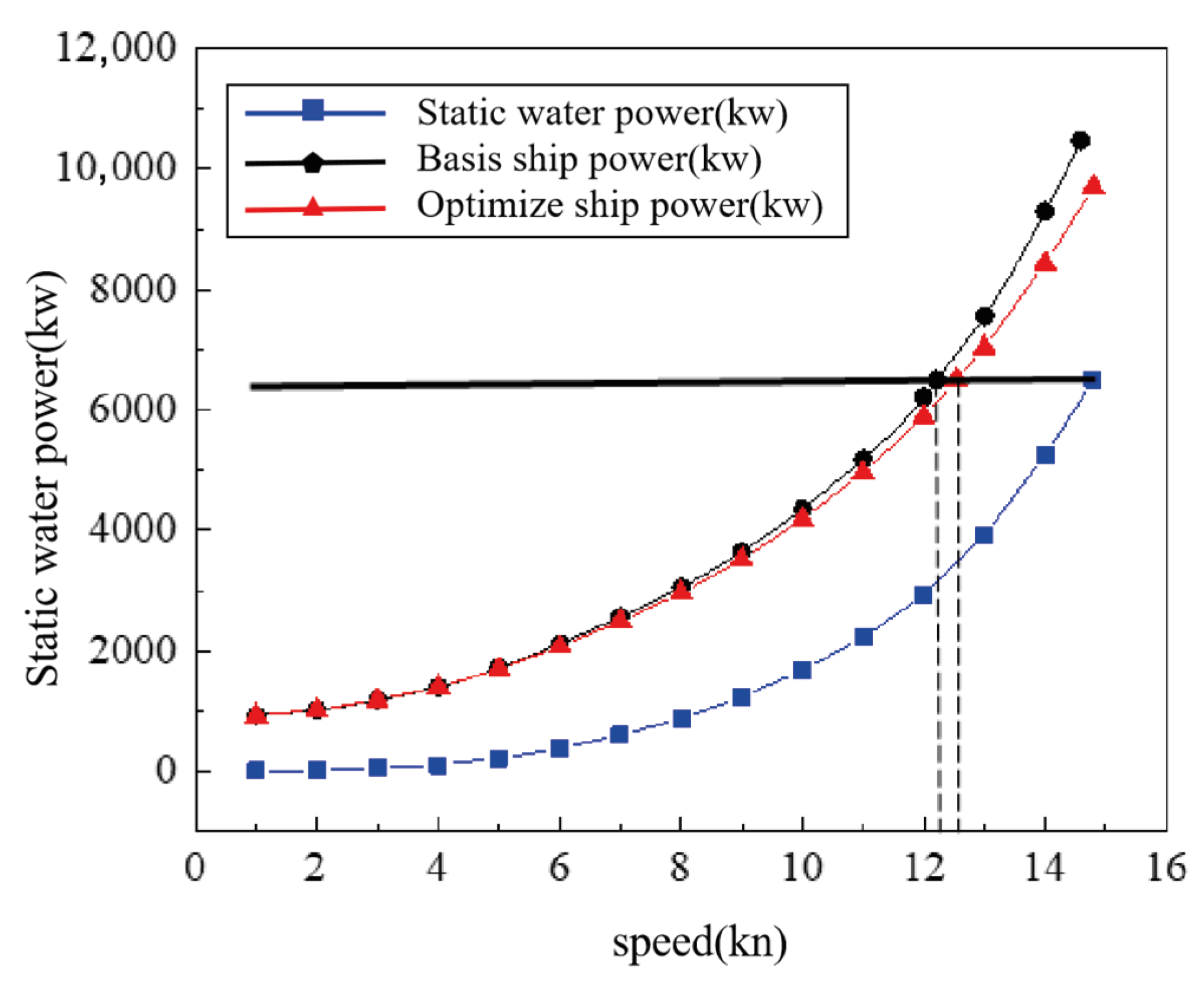
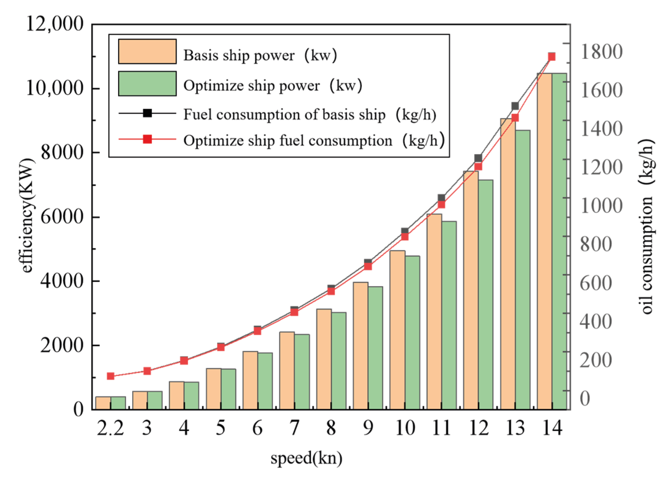
Figure 29.
Comparison of hydrostatic power and fuel consumption between basis and optimized ships.
Figure 29.
Comparison of hydrostatic power and fuel consumption between basis and optimized ships.
Figure 30.
Wind and wave stall comparison of basis and optimized ship.
Figure 30.
Wind and wave stall comparison of basis and optimized ship.
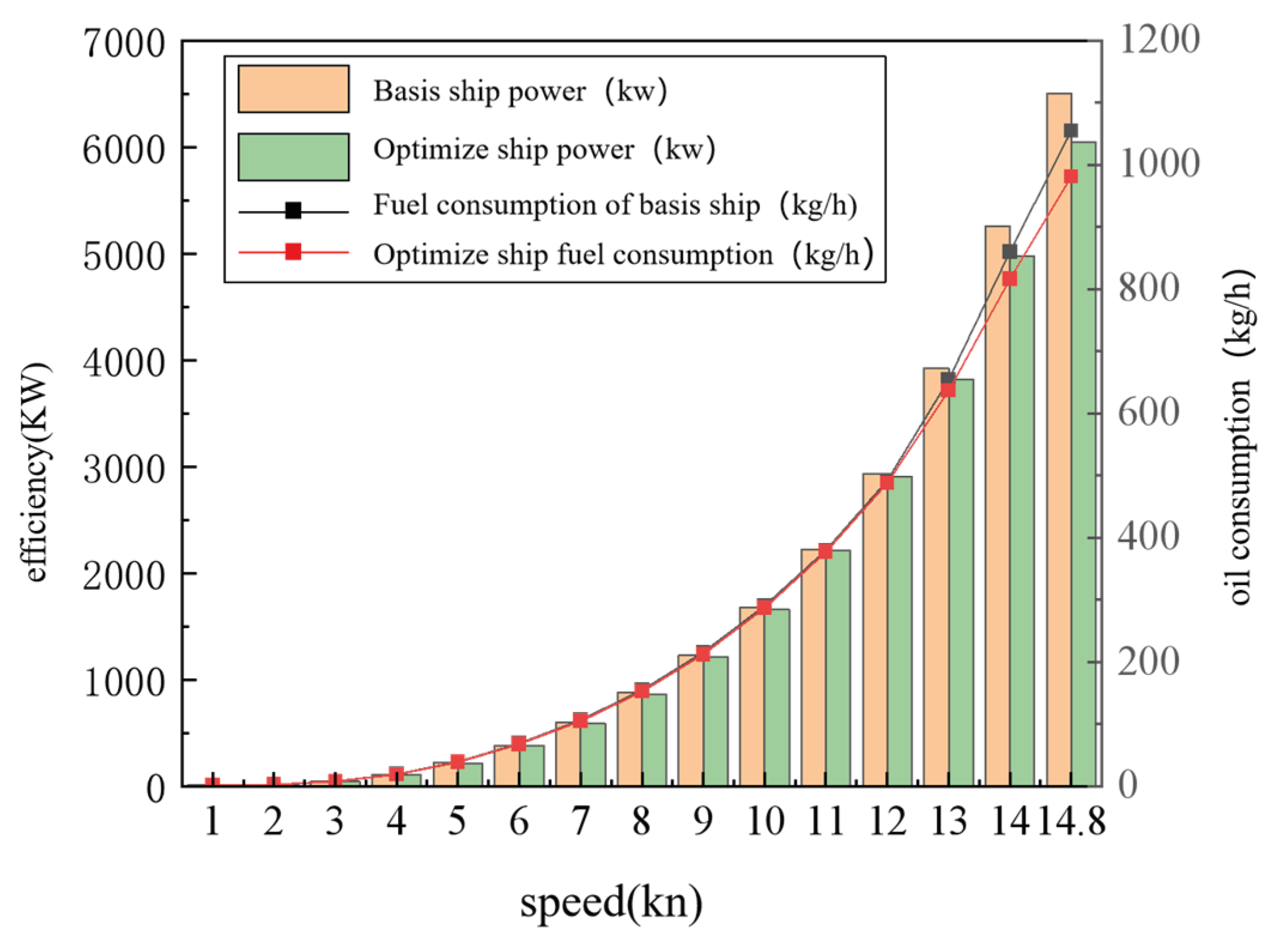
Figure 31.
Comparison of power and fuel consumption in the ice area between basis and optimized ships.
Figure 31.
Comparison of power and fuel consumption in the ice area between basis and optimized ships.
Table 1.
Parameters related to the target vessel.
Table 1.
Parameters related to the target vessel.
| No. | Category | Symbol | Vessel Parameters |
|---|
| 1 | Total length of ship | LOA (m) | 189.99 |
| 2 | Length between vertical lines | LPP (m) | 186.4 |
| 3 | Moulded Breadth | B (m) | 28.5 |
| 4 | Moulded Depth | D (m) | 15.8 |
| 5 | Average Draft | d (m) | 11 |
| 6 | Design Speed | Vs (kn) | 14.8 |
| 7 | Deadweight Tonnage | DWT (t) | 37125 |
| 8 | Square Coefficient | CB | 0.7904 |
| 9 | Prism Coefficient | CP | 0.8218 |
Table 2.
Wind and Wave Dataset.
Table 2.
Wind and Wave Dataset.
| Variable | Parameter | Unit | Definition/Description |
|---|
| Wind | 10 m U-component | m/s | Horizontal velocity of air moving eastward at 10 m above Earth’s surface. |
| 10 m V-component | m/s | Horizontal velocity of air moving northward at 10 m above the Earth’s surface. |
| Waves | Mean zero-crossing period | s | Average time interval between consecutive upward crossings of the mean sea level by waves. |
| Significant height of wind waves | m | Average height of the highest one-third of wind-generated waves at the ocean surface. |
Table 3.
Sea ice thickness classification.
Table 3.
Sea ice thickness classification.
| Type | Thickness/m |
|---|
| New Ice | <0.10 |
| Grey Pancake | 0.10–0.15 |
| Grey-White Ice | 0.15–0.30 |
| First-stage Thin First-year Ice | 0.30–0.50 |
| Second-stage Thin First-year Ice | 0.50–0.70 |
| Medium-thick First-year Ice | 0.70–1.20 |
| Thick First-year Ice | >1.20 |
| Two-year Ice | >2.50 |
| Multi-year Ice | >3.00 |
Table 4.
Ice density type.
Table 4.
Ice density type.
| Type | Ice Density | Navigation Condition |
|---|
| Nil ice | 0/10 | Unassisted navigation |
| Open water | <1/10 | Unassisted navigation |
| Very open ice | 1/10–3/10 | Course maintenance not guaranteed |
| Open ice | 4/10–6/10 | Navigation impeded |
| Medium ice | 7/10–8/10 | Navigation impeded |
| Close ice | 9/10 | Icebreaker assistance required |
| Very close ice | 9/10–10/10 | Icebreaker assistance required |
| Fast ice | 10/10 | No navigation possible without icebreaker |
Table 5.
Sea Ice Dataset.
Table 5.
Sea Ice Dataset.
| Data Source | Variable | Unit | Temporal Resolution | Spatial Resolution | Grid Size |
|---|
| University of Bremen | Sea ice concentration | — | Daily | 6.25 km | 1792 × 1216 |
| National Snow and Ice Data Center (NSIDC) | Sea ice thickness | m | Monthly | 25 km | 448 × 304 |
Table 6.
Basic curves of stern form.
Table 6.
Basic curves of stern form.
| NO. | Curve | Symbol |
|---|
| 1 | Deck at side | Deck |
| 2 | Flat edge line | Fos |
| 3 | Flat bottom line | Fob |
| 4 | Y value flat bottom line | YFob |
Table 7.
Basic curves of skeg form.
Table 7.
Basic curves of skeg form.
| Curve | Symbol |
|---|
| Skeg shape characteristic line1 | Skegshape1 |
| Skeg shape characteristic line2 | Skegshape2 |
| Tail shaft outlet cross-section shape | bossingshape |
| Tangent curve | CurveForTan |
| Caudal fin edge curve | SkegEdge |
Table 8.
Basic variables describing hull deformation.
Table 8.
Basic variables describing hull deformation.
| Variables | Symbol | Design Range |
|---|
| Longitudinal coordinate increment of floating center | △Xcb | −0.01~0.01 |
| Prism coefficient increment | △Cp | −0.1~0.05 |
| Fullness of bulbous bow | Bow-fullness | −2.5~2.5 |
| Caudal fin fullness | Skeg-fulness | −1~4 |
Table 9.
Regional voyage proportion.
Table 9.
Regional voyage proportion.
| Type | Range (n Mile) | Proportion |
|---|
| Open water area | 7383 | 0.91 |
| Ice area | 713 | 0.09 |
Table 10.
The proportion of ice conditions in the area.
Table 10.
The proportion of ice conditions in the area.
| Ice Thickness | Ice Concentration | Proportion |
|---|
| 0–0.3 | 10% | 0.12 |
| 0.3–0.6 | 50% | 0.42 |
| 0.6–0.9 | 3.30% | 0.32 |
| 0.9–1.2 | 40% | 0.14 |
Table 11.
The proportion of waves in the region.
Table 11.
The proportion of waves in the region.
| T (s) | 2 | 2.2 | 3 | 3 | 5.4 | 6 |
| Wave Height (m) | 2.27 | 2 | 3.34 | 4 | 5.35 | 5 |
| Proportion | 0.147 | 0.197 | 0.255 | 0.104 | 0.182 | 0.115 |
Table 12.
The proportion of wind conditions within the area.
Table 12.
The proportion of wind conditions within the area.
| Wind Scale | 2 | 3 | 4 | 5 | 6 |
| Wind Direction | Headwind | Tailwind | Headwind | Tailwind | Crosswind | Headwind | Tailwind | Headwind | Tailwind | Crosswind | Headwind |
| Proportion | 0.035 | 0.189 | 0.078 | 0.22 | 0.05 | 0.035 | 0.189 | 0.078 | 0.22 | 0.05 | 0.035 |
Table 13.
Calm water resistance calculation results.
Table 13.
Calm water resistance calculation results.
| Speed (KN) | Basis Ship Resistance (KN) | Optimized Ship Resistance (KN) | Optimization Rate |
|---|
| 2 | 8.71 | 8.604 | 1.22% |
| 4 | 31.692 | 31.307 | 1.22% |
| 6 | 74.904 | 73.976 | 1.24% |
| 8 | 128.842 | 127.251 | 1.24% |
| 10 | 198.022 | 196.112 | 0.97% |
| 12 | 287.544 | 285.63 | 0.67% |
| 14.8 | 502.862 | 473.085 | 5.92% |
Table 14.
Wave resistance calculation results.
Table 14.
Wave resistance calculation results.
| Wave height (m) | 2.27 | 2 | 3.34 | 4 | 5.35 | 5 |
| Cycle (s) | 2 | 2.2 | 3 | 3 | 5.4 | 6 |
| Basis ship resistance (KN) | 202.685 | 200.251 | 272.583 | 276.719 | 499.682 | 626.388 |
| Optimized ship resistance (KN) | 194.975 | 195.632 | 199.684 | 200.172 | 397.172 | 498.546 |
| Optimization rate | 0.038 | 0.023 | 0.267 | 0.276 | 0.205 | 0.204 |
Table 15.
Sea ice material parameters.
Table 15.
Sea ice material parameters.
| | Sea Ice Material
Parameters | Value | | Sea Ice Material
Parameters | Value |
|---|
| 1 | Density | 917 kg/m3 | 6 | Ship-ice friction coefficient | 0.05 |
| 2 | Diameter | 0.1~0.35 m | 7 | Yang’s modulus | 0.8 × 10⁹ pa |
| 3 | Thickness | 0.02 m | 8 | normal spring stiffness | 200 N/m |
| 4 | Poisson ratio | 0.3 | 9 | Tangential spring
stiffness | 200 N/m |
| 5 | Ice-ice friction
coefficient | 0.35 | 10 | | |
Table 16.
Interactions between phases.
Table 16.
Interactions between phases.
| Interactions Between Phase | Major Phase | Second Phase |
|---|
DEM particles and
DEM particles | DEM particles (ice) | DEM particles (ice) |
| DEM particles and solid wall | DEM particles (ice) | solid wall (ship) |
DEM particles and
VOF phase | DEM particles (ice) | VOF phase (water) |
| VOF phase and VOF phase | VOF phase (water) | VOF phase (air) |
Table 17.
Ice-breaking resistance calculation condition.
Table 17.
Ice-breaking resistance calculation condition.
| Working Condition | Ice Thickness (m) | Ice Density | Radius (m) | Speed (m/s) |
|---|
| 1 | 0.0215 | 40% | 0.15 | 0.6 |
| 2 | 0.015 | 30% |
| 3 | 0.0107 | 50% |
| 4 | 0.006 | 10% |


