Article

Fault Signal Emulation of Marine Turbo-Rotating Systems Based on Rotor-Gear Dynamic Interaction Modeling

1
Department of Autonomous Vehicle System Engineering, Chungnam National University, Daejeon 34134, Republic of Korea
2
Hanwha Ocean Co., Ltd., Seoul 04527, Republic of Korea
*
Author to whom correspondence should be addressed.
J. Mar. Sci. Eng. 2025, 13(7), 1321; https://doi.org/10.3390/jmse13071321
Submission received: 11 June 2025 / Revised: 2 July 2025 / Accepted: 8 July 2025 / Published: 9 July 2025
(This article belongs to the Section Ocean Engineering)

Abstract

Rotating machinery is essential in various industrial fields, and growing demands for high performance under harsh operating conditions have heightened interest in fault diagnosis and prognostic technologies. However, a major challenge in fault diagnosis research lies in the scarcity of data, primarily due to the inability to deliberately introduce faults into machines during actual operation. In this study, a physical model is proposed to realistically simulate the system behavior of a ship’s turbo-rotating machinery by coupling the torsional and lateral vibrations of the rotor. While previous studies employed simplified single-shaft models, the proposed model adopted gear mesh interactions to reflect the coupling behavior between shafts. Furthermore, the time-domain response of the system is analyzed through state-space transformation. The proposed model was applied to simulate imbalance and gear teeth damage conditions that may occur in marine turbo-rotating systems and the results were compared with those under normal operating conditions. The analysis confirmed that the model effectively reproduces fault-induced dynamic characteristics. By enabling rapid implementation of various fault conditions and efficient data acquisition data, the proposed model is expected to contribute to enhancing the reliability of fault diagnosis and prognostic research.

1. Introduction

Rotating machinery plays an important role in a wide range of industrial applications, including power transmission, fluid compression, and electricity generation [1,2]. Faults in rotating machinery within large-scale industrial systems, such as transportation infrastructure or power plants, can lead not only to significant economic losses from equipment downtime but also to serious safety hazards resulting from mechanical failure. To detect faults in advance and to establish efficient maintenance strategies, extensive research has been conducted on PHM (prognostic and health management) and CBM (condition-based maintenance) [3].
Approaches for condition assessment are generally classified into physics-based methods and data-driven methods. Physics-based methods utilize the dynamic characteristics of a system by modeling its operation mechanism through mathematical equations [4,5]. Since data are only required for the model validation process, these methods offer the advantage of relatively low dependence on data. Meanwhile, data-driven methods do not consider the underlying dynamics of a system but instead diagnose its condition using sensor data acquired directly from the system. To accurately assess the conditions of a system, it is essential to acquire a large amount of data representing various operating states. In general, among various types of sensor data, data-driven approaches that utilize vibration signals are widely adopted, and they are effective in detecting fault symptoms in rotating machinery [6,7,8]. Recently, more accurate fault diagnosis has been achieved in practice through hybrid approaches that combine the strengths of both physics-based and data-driven methods [9,10,11,12].
Data-driven methods have been rapidly advancing, as they enable diagnosis of system states without requiring expertise in physical characteristics or systems. In particular, numerous diagnosis models utilizing artificial intelligence have been proposed to process enormous amounts of data that are beyond human comprehension [13,14,15,16,17]. However, there are still many limitations in obtaining sufficient data required for fault diagnosis research. If a fault intentionally implemented into real equipment for data acquisition leads to failure, it can result in serious economic losses and potential threats to human safety. In addition, it takes a lot of time and money to acquire sufficient data by simulating various fault situations. Due to these issues, the difficulty in acquiring data is a major obstacle to the advancement of fault diagnosis technology.
Therefore, many studies use open datasets with high accessibility. Representative open datasets include CWRU Bearing Set [18,19,20,21], IMS Bearing set [22,23], SEU gearbox dataset [24,25], and MFPT Bearing set [26,27]. However, there are the following limitations when using open data; Firstly, the generality of the research results cannot be guaranteed because the physical information about the subject from which the data was acquired is not known. Secondly, since the experimental environment cannot be perfectly reproduced, obtaining additional data is impossible. Lastly, most open datasets only simulate faults of specific mechanical elements, so information on various fault situations cannot be obtained. To overcome the limitations of open datasets, there are cases in which data are acquired directly by utilizing a testbed that simulates the faults of the target equipment [28,29,30,31,32]. However, these methods also have the limitation that it can only simulate faults of specific elements, and it takes a lot of time to acquire a large amount of data. Crucially, the testbed is a scaled-down version of the parent object, so additional verification of the physical correlation with the actual object is required.
A physics-based model can efficiently secure a large amount of data. A physics-based modeling approach was proposed to monitor the performance degradation of a gas turbine engine, and it was verified that the developed performance indicators can be used for condition prediction and predictive maintenance [33]. It was shown that multiple fault s can be detected, and the remaining life can be predicted by combining physics-based models to develop a diagnostic and prognostic model for the HVAC (heating, ventilation, and air conditioning) system inside a passenger train cabin where fault data is insufficient [34]. A new mathematical model for the complex interactions of components inside an aircraft engine system was developed, which significantly improved the prediction accuracy compared to using independent physical models of each element [35]. Through the analysis of the dynamic behavior of a multi-stage parallel gearbox of TBM (Tunnel Boring Machines), a complex piece of equipment used in tunnel construction, it was verified that the most influential factors in the vibration amplification of the system are the impact force of the gear and the nonlinearity of the bearing [36].
The physics model-based approach can be extended to a simulator or digital twin system to quickly obtain data. A digital twin model was used to generate bearing fault data under various operating conditions, producing high-quality fault samples that were applied to a data-based diagnosis algorithm [37]. A virtual model was also built to obtain dynamic behavior data of a gearbox and was calibrated with real data to generate fault data [38]. In another case, a digital twin-based model was used to diagnose and predict rotor imbalance [39]. Additionally, fault data for data-based machine learning were generated by simulating fault signatures such as cracks in blade disks using a low-dimensional physics-based model [40]. However, many rotating machineries used in industrial sites have structures in which multiple shafts are connected by gear meshing. Existing studies have mainly used methods that simplify the rotating system into a simplified model, but they have limitations in accurately simulating the dynamic characteristics of the actual system because they do not sufficiently reflect the interactions between the shafts. In a multi-shaft system, since the vibration phenomenon of one shaft affects the behavior of the other shaft, the interactions between the shafts must be sufficiently reflected in order to accurately model the target system. Moreover, when configuring the simulator, the physical model was mainly designed either around a single component or with the goal of generating data for individual faults. Therefore, there is a limit to immediately acquiring a large amount of fault data or to rapidly securing learning data by continuously changing various system conditions.
In this study, we propose a framework that can quickly generate various fault data based on a physical model that reflects the coupled behavior of torsional vibration and lateral vibration in a complex multi- shafts rotating system. We implemented a 20-degree-of-freedom (DOF) physical model that effectively reflects the coupled behavior by applying a gear-meshing model and secured the analysis speed by simplifying the main mass using the concentrated inertia method during the modeling process. Additionally, we designed a GUI-based simulator that can quickly generate the time-series dynamic response of the system under fault conditions by converting the model into a state space form. By utilizing this, we confirmed that the fault characteristics were accurately expressed by comparing major faults such as mass imbalance and gear tooth damage with the normal state response. The user-friendly GUI simulator has the advantage of intuitively changing the main system parameters and performing simulations under various faults and operating conditions in real time. The proposed framework precisely simulates the behavior of multi-shaft coupled rotors while providing an environment for rapidly acquiring a large amount of fault data through state equation-based analysis. Therefore, it has high potential for use in verifying machine learning-based fault diagnosis algorithms and securing data for building digital twins and can contribute to improving the reliability of fault diagnosis research.
Meanwhile, a multi-shaft rotating system can inherently be interpreted as a dynamic mechanical network, where shafts, gears, and bearings act as nodes and their mechanical couplings serve as edges. This network perspective is essential for understanding fault propagation and the overall system dynamics. As demonstrated in various studies that applied network science to analyze complex interactions across different domains [41,42], our physics-based model holds the potential to be integrated with network-based analyses and learning approaches in the future, thereby serving as a solid foundation to further enhance the reliability of data-driven PHM and CBM.
The order of the paper is as follows. The structure and operation mechanism of the LNG re-liquefaction system (Compander), which is the research target ship turbo-rotor, are examined in Section 2. The shaft system modeling of the rotor is dealt with in Section 3, and the gear-meshing model is dealt with in Section 4. In Section 5, the time-domain signal is generated through the model converted to the state-space format, and the fault characteristics are analyzed. The simulator including the model developed in this study is described in Section 6, and finally, the conclusion and future research directions are discussed in Section 7.

2. LNG Re-Liquefaction System

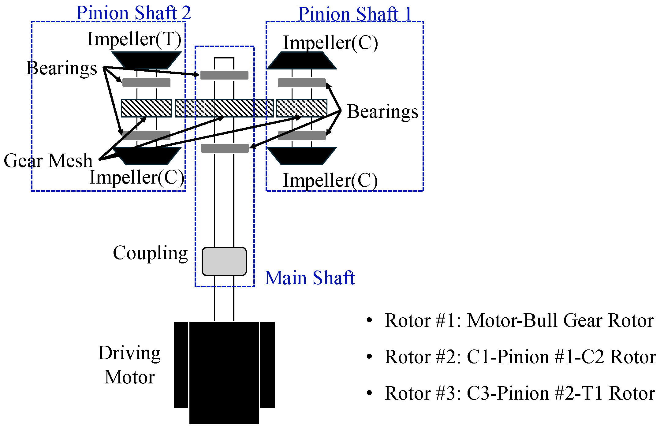
The subject of this study is equipment that re-liquefies BOG (Boil Off Gas) of LNG carriers or LNG propulsion ships into LNG, and as shown in Figure 1, it has a structure in which one main shaft and two auxiliary shafts are connected through a gear mesh [43]. This system re-liquefies LNG that has been vaporized by the reverse Brayton cycle, which is mainly used in refrigerators and aircraft. Nitrogen refrigerant is introduced into the front impeller of the right-hand pinion shaft 1, and after compressing the nitrogen-containing refrigerant through a three-stage compressor, it undergoes adiabatic expansion in the left-hand pinion shaft 1-stage expansion turbine and then re-liquefies BOG through a heat exchanger [44].
The main rotating elements that constitute the system include an electric motor that drives the main shaft, a compressor, an expansion turbine, gears, and bearings. The main shaft is connected to an electric motor that rotates at low speed and produces high torque, and the pinion shaft is rotated at high speed through a gear connection. To support the shafts, the main shaft uses two sleeve bearings, and the auxiliary shaft uses four tilting pad bearings. The pinion shaft connected to the main shaft by gears rotates at high speed and operates the compressor impeller and the expansion turbine. The pinion shafts are arranged one on each side of the main shaft, and each shaft receives an aerodynamic load due to the compressor and expander at the end. The structure of this LNG re-liquefaction system can be viewed as a typical multi-stage gear-type rotor structure. However, it is difficult to intuitively predict the system behavior because the response of the rotating shaft results from the combined effects of lateral and torsional vibrations of the three shafts, which are coupled through the gears at both ends. In this study, to predict the behavior of this system, we present a model that simplifies the structure and can solve the lateral vibration and torsional vibration in combination.

3. Rotor Vibration Model

3.1. Torsional Vibration Modeling

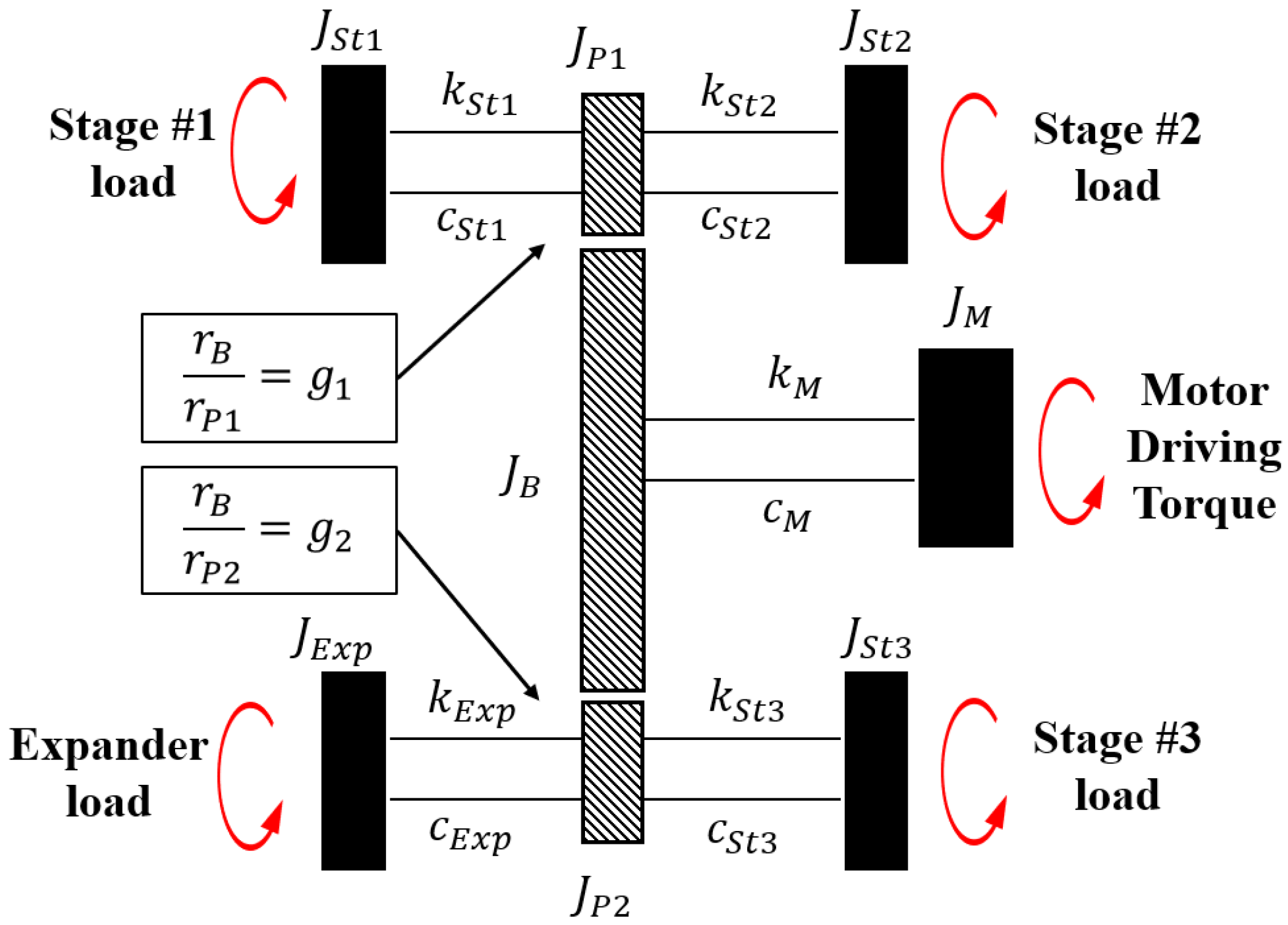
In an operating rotor, torsional vibration and lateral vibration occur simultaneously, and the two vibrations affect each other. The torsional vibration can be expressed by the rotational inertia, torsional stiffness, damping, and the load applied to the rotor. In this study, we attempted to shorten the analysis time by discretizing the major mass elements using lumped inertia-based modeling. Using the lumped inertia method, torque transmission is modeled by the stiffness and damping of the rotating shaft, and the DOF of the rigid shaft or gear can be efficiently reduced [45]. The target system is represented by rotational inertia and the stiffness and damping of the rotating shaft, as shown in Figure 2. The torsional vibration model has angular values for the eight lumped inertias expressed in Equation (1) as variables.
Θ = { θ M , θ B , θ P 1 , θ P 2 , θ S t 1 , θ S t 2 , θ S t 3 , θ E x p } T
By substituting the kinetic energy (T) and potential energy (V) of the concentrated inertia expressed in terms of the torsional angle into the Lagrange equation of Equation (2), the relationship between the non-conservative force ( Q n ) for each lumped inertia in the torsional vibration model can be derived.
d d t L θ ˙ n L θ n = Q n , L = T V  
The equations of motion, including the results derived from the Lagrange equation, can be expressed in terms of inertia, damping, stiffness, and torque vectors as follows. The subscript t indicates a value related to torsional vibration. Additionally, { T } represents the external force (torque) matrix.
[ J ] Θ ¨ + [ C t   ] Θ ˙ + [ K t ] Θ = { T }
At this time, to reduce the model variables, the fixed angular ratios for the main gear and two pinion gears of the system can be defined as follows.
g 1 θ B = θ P 1 , g 1 = r B r P 1
g 2 θ B = θ P 2 , g 2 = r B r P 2
Each matrix constituting Equation (3) can be expressed as Equations (6)–(9) to obtain a torsional vibration model of the LNG re-liquefaction system.
J = J M 0 0 0 0 0 0 J B + J P 1 g 1 2 + J P 2 g 2 2 0 0 0 0 0 0 J S t 1 0 0 0 0 0 0 J S t 2 0 0 0 0 0 0 J S t 3 0 0 0 0 0 0 J E x p
K t = k t , M k t , M 0 0 0 0 k t , M ( k t , M + k t , S t 1 g 1 2 + k t , S t 2 g 1 2 + k t , S t 3 g 2 2 + k t , E x p g 2 2 ) k t , S t 1 g 1 k t , S t 2 g 1 k t , S t 3 g 2 k t , E x p g 2 0 k t , S t 1 g 1 k t , S t 1 0 0 0 0 k t , S t 2 g 1 0 k t , S t 2 0 0 0 k t , S t 3 g 2 0 0 k t , S t 3 0 0 k t , E x p g 2 0 0 0 k t , E x p
C t = ( c t , M + B t , M ) c t , M 0 0 0 0 c t , M c t , T c t , S t 1 g 1 c t , S t 2 g 1 c t , S t 3 g 2 c t , E x p g 2 0 c t , S t 1 g 1 2 ( c t , S t 1 + B t , S t 1 ) 0 0 0 0 c t , S t 2 g 1 2 0 ( c t , S t 2 + B t , S t 2 ) 0 0 0 c t , S t 3 g 2 2 0 0 ( c t , S t 3 + B t , S t 3 ) 0 0 c t , E x p g 2 2 0 0 0 ( c t , E x p + B t , E x p )
c T = ( c t , M + c t , S t 1 g 1 2 + c t , S t 2 g 1 2 + c t , S t 3 g 2 2 + c t , E x p g 2 2 + B t , B + B t , P 1 g 1 2 + B t , P 2 g 2 2 )

3.2. Lateral Vibration Modeling

There are several methods for modeling the lateral vibration of a rotating body, such as the lumped inertia model, the transfer function model, and the finite element model. In this study, the lumped inertia model was used to secure the speed of analysis. When the lumped inertia is applied, a simple lateral vibration model with four DOF of the translational motion in the x and y directions and the rotational motions α and β can be expressed as in Figure 3. The lateral vibration model includes the gyroscopic effect of the rotational axis, and the model for one shaft has four DOF. In the following, the subscript L indicates the component related to lateral vibration. Here, vibration caused by bending is neglected. It is generally recognized in rotor dynamics that the bending of short, rigid shafts can be safely ignored [46]. However, it should be noted that for flexible body models or long-shaft structures, this assumption needs to be reconsidered.
If the lateral modeling is performed for three shafts, as shown in Figure 4, based on one main gear and two pinion gears with the largest inertia in the compander, the lateral vibration model is expressed as a model with 12 DOF. However, the lateral vibration model for each shaft does not reflect the influence among them. To reflect the coupling between the shafts that occur in the real system, modeling of the gear elements that transmit force and moment is required. Equations (10)–(21) represent the lateral vibration model of the system. A more detailed derivation of the equations of motion for a rotating body that includes the gyroscopic term can be found in [46].
m B x ¨ B + k B , x 1 x B α B a B + k B , x 2 x B + α B b B + k B , x 1 y 1 y B + β B a B + k B , x 2 y 2 ( y B β B b B ) = 0
m B y ¨ B + k B , y 1 y B + β B a B + k B , y 2 y B β B b B + k B , y 1 x 1 x B α B a B + k B , y 2 x 2 ( x B + α B b B ) = 0
I B , T β ¨ B + k B , y 1 y B + β B a B a B k B , y 2 y B β B b B b B + k B , y 1 x 1 x B α B a B a B k B , y 2 x 2 x B + α B b B b B + I B , P ω B α ˙ B = 0
I B , T α ¨ B k B , x 1 x B α B a B a B + k B , x 2 x B + α B b B b B k B , x 1 y 1 y B + β B a B a B + k B , x 2 y 2 y B β B b B b B I B , P ω B β ˙ B = 0
m P 1 x ¨ P 1 + k P 1 , x 1 x P 1 α P 1 a P 1 + k P 1 , x 2 x P 1 + α P 1 b P 1 + k P 1 , x 1 y 1 y P 1 + β P 1 a P 1 + k P 1 , x 2 y 2 ( y P 1 β P 1 b P 1 ) = 0
m P 1 y ¨ P 1 + k P 1 , y 1 y P 1 + β P 1 a P 1 + k P 1 , y 2 y P 1 β P 1 b P 1 + k P 1 , y 1 x 1 x P 1 α P 1 a P 1 + k P 1 , y 2 x 2 ( x P 1 + α P 1 b P 1 ) = 0
I P 1 , T β ¨ P 1 + k P 1 , y 1 y P 1 + β P 1 a P 1 a P 1 k P 1 , y 2 y P 1 β P 1 b P 1 b P 1 + k P 1 , y 1 x 1 x P 1 α P 1 a P 1 a P 1 k P 1 , y 2 x 2 ( x P 1 + α P 1 b P 1 ) b P 1 + I P 1 , P ω P 1 α ˙ P 1 = 0
I P 1 , T α ¨ P 1 k P 1 , x 1 x P 1 α P 1 a P 1 a P 1 + k P 1 , x 2 x P 1 + α P 1 b P 1 b P 1 k P 1 , x 1 y 1 y P 1 + β P 1 a P 1 a P 1 + k P 1 , x 2 y 2 y P 1 β P 1 b P 1 b P 1 I P 1 , P ω P 1 = 0
m P 2 x ¨ P 2 + k P 2 , x 1 x P 2 α P 2 a P 2 + k P 2 , x 2 x P 2 + α P 2 b P 2 + k P 2 , x 1 y 1 y P 2 + β P 2 a P 2 + k P 2 , x 2 y 2 ( y P 2 β P 2 b P 2 ) = 0
m P 2 y ¨ P 2 + k P 2 , y 1 y P 2 + β P 2 a P 2 + k P 2 , y 2 y P 2 β P 2 b P 2 + k P 2 , y 1 x 1 x P 2 α P 2 a P 2 + k P 2 , y 2 x 2 ( x P 2 + α P 2 b P 2 ) = 0
I P 2 , T β ¨ P 2 + k P 2 , y 1 y P 2 + β P 2 a P 2 a P 2 k P 2 , y 2 y P 2 β P 2 b P 2 b P 2 + k P 2 , y 1 x 1 x P 2 α P 2 a P 2 a P 2 k P 2 , y 2 x 2 ( x P 2 + α P 2 b P 2 ) b P 2 + I P 2 , P ω P 2 α ˙ P 2 = 0
I P 2 , T α ¨ P 2 k P 2 , x 1 x P 2 α P 2 a P 2 a P 2 + k P 2 , x 2 x P 2 + α P 2 b P 2 b P 2 k P 2 , x 1 y 1 y P 2 + β P 2 a P 2 a P 2 + k P 2 , x 2 y 2 ( y P 2 β P 2 b P 2 ) b P 2 I P 2 , P ω P 2 β ˙ P 2 = 0

3.3. Bearing Modeling

The lateral vibration of a rotor is greatly affected by the stiffness and damping of the bearings supporting the rotor. The compander is supported by two sleeve bearings (main shaft) and four tilting pad bearings (auxiliary shaft), and since the axial response is not considered in the lateral vibration model, the stiffness and damping of the bearings are expressed by Equation (23). The subscripts x x and y y represent the respective axial material properties, and x y and y x represent the mutual coupling in different directions.
C b r g = c x x c x y c y x c y y , K b r g = k x x k x y k y x k y y
In the case of sleeve bearings, the nondimensional stiffness and damping are obtained by assuming a fully cavitated (π-film) short bearing based on the Eccentricity Ratio (ε) value [47], and the nondimensional stiffness and damping are then converted into dimensional values based on the rotational speed and rated load. To simplify modeling, two sleeve bearings are modeled with the same stiffness and damping, which are shown in Table 1. In the case of tilting pad bearings, the dimensional stiffness and damping values were derived using the nondimensional values [48] that reflect the geometric information of the bearing, and the values are shown in Table 2. Here, stiffness has units of N/m and damping has units of N∙s/m.
The stiffness and damping values for the six calculated fluid bearings are applied to the lateral vibration model.

4. Gear-Meshing Model

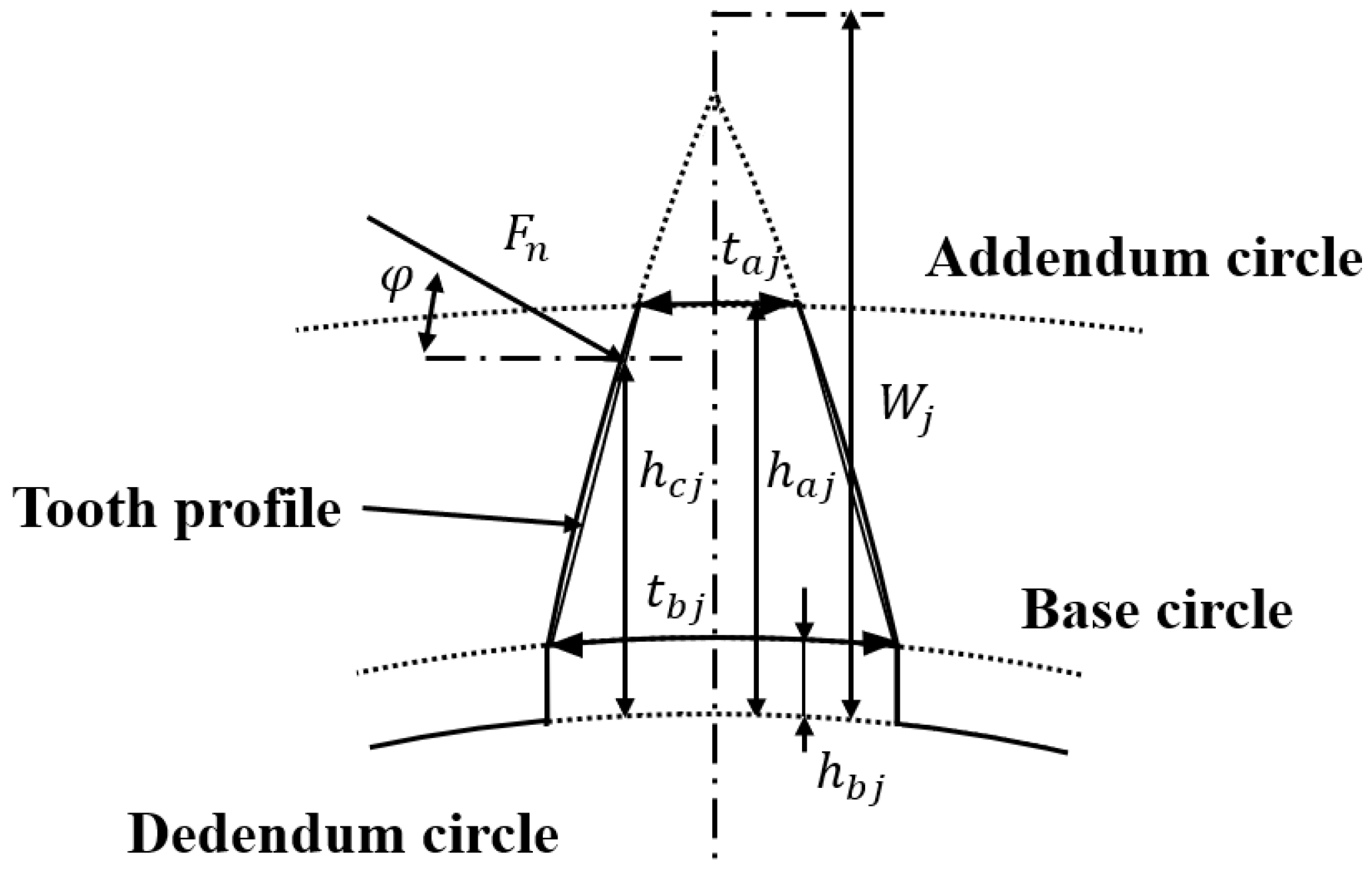
In multi-shaft rotating equipment, gears not only couple the torsional and lateral vibrations of each shaft but also transmit the forces and moments of one shaft to the others. The gear connection can be modeled as the meshing between gear teeth, which is expressed in terms of stiffness and damping. Figure 5 shows the geometry and parameters of gear teeth [49]. The addendum circle is a circle that includes the tip of the gear tooth and determines the outer diameter of the gear. The dedendum circle is a circle that includes the root of the gear tooth and defines the lowest part of the gear tooth profile. The distance between the dedendum circle and the addendum circle determines the height of the gear tooth, which affects the durability and wear characteristics of the gear. The base circle is a circle that determines the gear tooth profile. The tooth profile represents the overall shape of the gear tooth and is a key factor in determining the meshing characteristics of the gear.
The bending strain ( δ b p j ) due to the horizontal contact force of the gear teeth, the bending strain ( δ b n j ) due to the vertical contact force, the shear strain ( δ s j ), the strain due to the bending of the gear teeth ( δ f j ), and the compressive strain due to the contact ( δ h j ), which are generated due to the force transmitted as the gears mesh, can be calculated based on the following formula using the shape parameters of the gear teeth defined based on the aforementioned circles.
ω j = h a j t b j h b j t a j t b j t a j
δ b p j = 12 F n c o s 2 φ h b j E f t b j 3 h c j 2 + h b j 2 3 h c j h b j + 6 F n c o s 2 φ ( ω j h b j ) 3 E f t b j 3 [ ω j h c j ω j h b j ( 4 ω j h c j ω j h b j ) 2 l n ω j h c j ω j h b j 3 ]
δ b n j = 3 F n c o s φ s i n φ E f t b j 2 [ h b j ( h b j 2 h c j ) ( ω j h c j ) ω j h b j ( h c j h b j ) 2 ]
δ s j = 1.2 F n c o s 2 φ G f t b j [ h b j + ( ω j h b j ) l n ω j h b j ω j h c j ]
δ f j = 24 F n c o s 2 φ h c j 2 π E f t b j 2
δ h j = 4 F n ( 1 ν 2 ) π E f
The gear-meshing stiffness coefficient can be obtained through the deformation occurring in the gear. The meshing situation of the gears can be assumed by distinguishing between the case where one pair of gear teeth meshes and the case where two pairs of gear teeth mesh. In this study, it was assumed that two pairs of gear teeth meshed, and the gear stiffness expressed in Equation (29) was calculated as a parallel connection.
k j = F n δ j , t o t a l = F n δ b n j + δ b p j + δ s j + δ f j + δ h j
The transmission power between gears can be defined using the difference in displacement and rotation angle of the two connected shafts, and assuming that there is no meshing damping, the transmission power by gear meshing can be expressed as follows.
F n = k h { ( u 2 g u 1 g ) s i n φ + ( v 2 g v 1 g ) c o s φ ( r 1 θ 1 g + r 2 θ 2 g ) }
F n u 1 = F n s i n φ = k h [ s i n 2 φ s i n φ c o s φ 0 0 r 1 s i n φ s i n 2 φ s i n φ c o s φ 0 0 r 2 s i n φ ] [ q ] g
F n v 1 = F n s i n φ = k h [ s i n φ c o s φ c o s 2 φ 0 0 r 1 c o s φ s i n φ c o s φ c o s 2 φ 0 0 r 2 c o s φ ] [ q ] g
The gear-meshing–force relationship defined above was added as a transmission force to the torsional vibration model and the lateral vibration model of the rotor, and the coupling between the torsional and lateral vibration models as well as the coupling between the lateral vibration models of the three shafts was reflected. The equations of motion of the system reflecting the gear coupling are given as follows. In this context, the model variable reduction through Equations (4) and (5) is not reflected in order to individually examine the response of each variable.
m x ¨ B + k B , x 1 x B α B a B + k B , x 2 x B + α B b B + k B , x 1 y 1 y B + β B a B + k B , x 2 y 2 y B β B b B F h x B 1 F h x B 2 = 0
m y ¨ B + k B , y 1 y B + β B a B + k B , y 2 y B β B b B + k B , y 1 x 1 x B α B a B + k B , y 2 x 2 x B + α B b B F h y B 1 F h y B 2 = 0
m x ¨ P 1 + k P 1 , x 1 x P 1 α P 1 a P 1 + k P 1 , x 2 x P 1 + α P 1 b P 1 + k P 1 , x 1 y 1 y P 1 + β P 1 a P 1 + k P 1 , x 2 y 2 ( y P 1 β P 1 b P 1 ) + F h x B 1 = 0
m y ¨ P 1 + k P 1 , y 1 y P 1 + β P 1 a P 1 + k P 1 , y 2 y P 1 β P 1 b P 1 + k P 1 , y 1 x 1 x P 1 α P 1 a P 1 + k P 1 , y 2 x 2 ( x P 1 + α P 1 b P 1 ) + F h y B 1 = 0
m x ¨ P 2 + k P 2 , x 1 x P 2 α P 2 a P 2 + k P 2 , x 2 x P 2 + α P 2 b P 2 + k P 2 , x 1 y 1 y P 2 + β P 2 a P 2 + k P 2 , x 2 y 2 ( y P 2 β P 2 b P 2 ) + F h x B 2 = 0
m y ¨ P 2 + k P 2 , y 1 y P 2 + β P 2 a P 2 + k P 2 , y 2 y P 2 β P 2 b P 2 + k P 2 , y 1 x 1 x P 2 α P 2 a P 2 + k P 2 , y 2 x 2 ( x P 2 + α P 2 b P 2 ) + F h y B 2 = 0
J B θ ¨ B k M ( θ M θ B ) c M ( θ ˙ M θ ˙ B ) + B B θ ˙ B + T B 1 + T B 2 = 0
J P 1 θ ¨ p g 1 + k S t 1 θ P 1 θ P 1 + k S t 2 θ P 1 θ P 2 + c S t 1 θ ˙ P 1 θ ˙ S t 1 + c S t 2 θ ˙ P 1 θ ˙ S t 2 + B p g 1 θ ˙ p g 1 T p g 1 = 0
J P 2 θ ¨ P 2 + k S t 3 θ P 2 θ S 3 + k E x p θ P 2 θ E x p + c S t 3 θ ˙ P 2 θ ˙ S t 3 + c E x p θ ˙ P 2 θ ˙ E x p + B P 2 θ ˙ P 2 T P 2 = 0

5. Model Analysis Result

To analyze the dynamic behavior of the model proposed in this study in the time domain, the three-shaft rotational model was converted into a state-space form. This enables for more efficient analysis of the time series response of the system and analysis by simulating various fault conditions.

5.1. State-Space Model

Both the torsional vibration model and the lateral vibration model presented in the previous chapter are coupled by substituting the force and moment equations due to the gear meshing. The system is expressed by 20 equations of motion consisting of 20 model variables.
q = { x B   y B   α B   β B   θ B   x P 1   y P 1   α P 1   β P 1   θ P 1   x P 2   y P 2   α P 2   β P 2   θ P 2   θ M   θ S t 1   θ S t 2   θ S t 3   θ E x p   } T
The 20 equations organized in matrix form are as follows.
M 20 × 20 q ¨ 20 × 1 + D 20 × 20 q ˙ 20 × 1 + K 20 × 20 q 20 × 1 = [ F ] 20 × 1
If this is converted into a state-space format, it can be expressed as Equation (44).
X ˙ = A X + B U Y = C X + D U
In this equation, X is a vector consisting of model variables of the system, U is an input vector, and Y is an output vector. The A, B, C, and D matrices representing the dynamic characteristics of the system are defined as follows.
A = 0 I M 1 K M 1 D 40 × 40 , B = 0 M 1 40 × 20 , C = I   0 20 × 40 , D = 0 20 × 20
Here, M, D and K are the inertia matrix, damping matrix, and stiffness matrix that reflect both torsional vibration and lateral vibration, and I is the unit matrix.
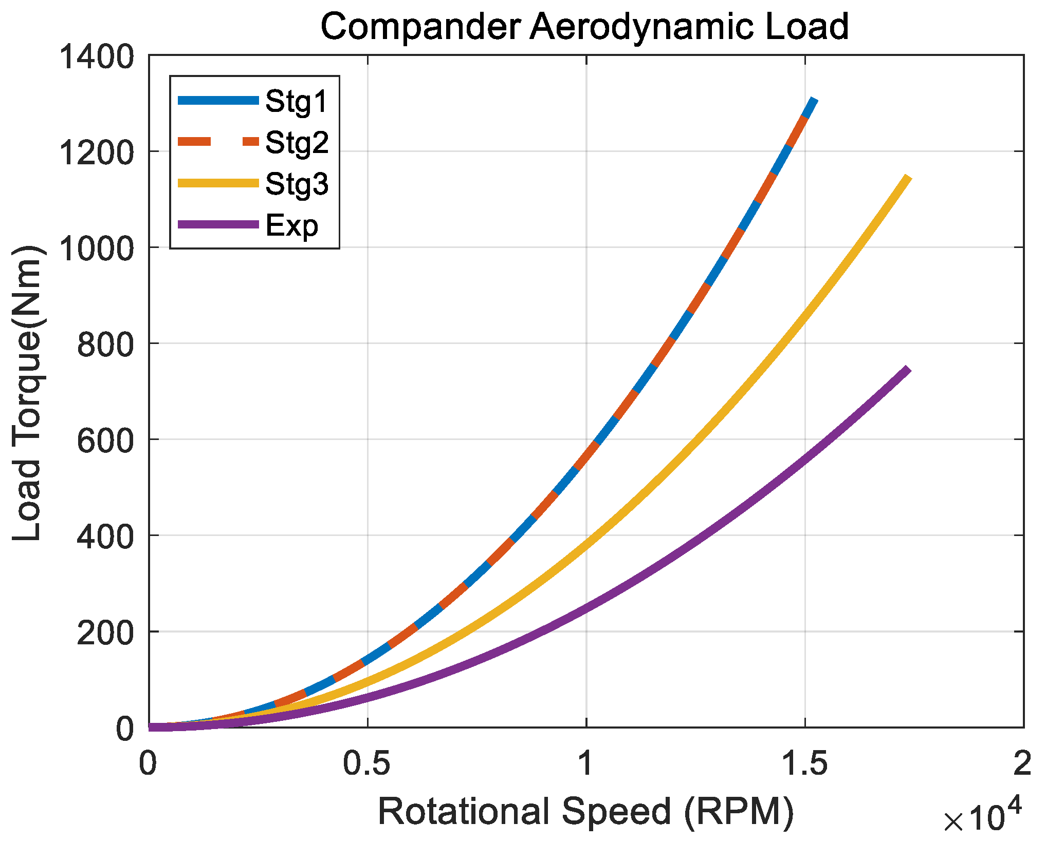
The torque input values of the model are the motor output, compressor, and expander loads. The motor provides torque so that it can rotate at the required speed through the current speed-based feedback control with the maximum torque as the limit. The compressor and expander models were modeled based on the maximum operating point, assuming that the aerodynamic load is proportional to the square of the impeller rotational speed, as shown in Figure 6 [50].
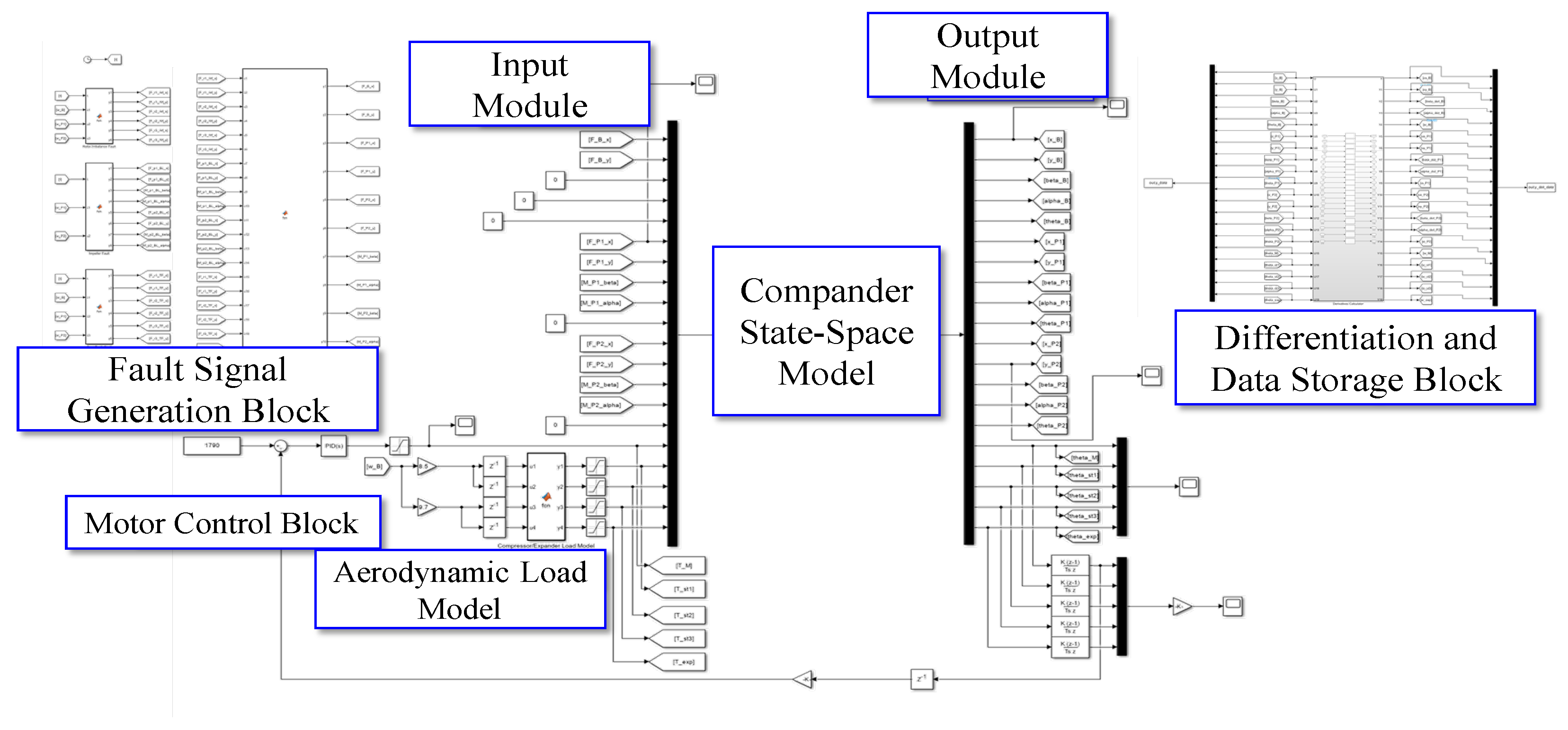
The time-series response generation system that implements the state-space model in the MATLAB/Simulink (MATLAB R2023a) environment is shown in Figure 7. The simulator consists of an input module, an output module, a fault signal generation block, a motor control block, an aerodynamic load model, and differentiation and data storage blocks according to their main functions. The compander state-space model, which is a core element, converts a three-shaft rotational system that considers gear meshing into a state-space format and calculates the dynamic response of a physical model in which both torsional and lateral vibrations are coupled. The results are transmitted through the output module, and the data required for analysis can be post-processed using differentiation and data storage blocks. Through this structure, the simulator can generate data of various states for fault diagnosis and prediction studies.

5.2. Response Analysis of Fault Conditions

The impeller, bearing, rotating shaft, and gear that constitute the compander are known as representative components that cause failure of the rotating body [51,52]. In this study, the response under imbalance and gear fault conditions was verified. Since these are typical faults that frequently occur in rotating machinery, in-depth analysis is required to ensure stable operation. In addition, since there is a clear numerical verification procedure, it is useful for reproducing the fault mechanisms in similar multi-shaft systems. The model was converted into a state-space format to generate time series data of fault conditions, and the system behavior under fault conditions was analyzed through the vibration response of the system, frequency spectrum, and orbit plot.

5.2.1. Imbalance Simulation

The main causes of imbalance are material loss, poor balancing correction, and adsorption of foreign substances, and they may also be secondary causes of impeller or gear loss or wear. The eccentricity of the mass acts as a harmonic excitation force on the x and y axes of the lateral vibration model. Equations (46) and (47) are equations that express the imbalance force for the imbalance amount e r existing on the main shaft as a harmonic excitation force.
F r , x = m r e r ω r 2 c o s ω r t
F r , y = m r e r ω r 2 s i n ( ω r t )
In this equation, m r applied the allowable residual imbalance of the machine calculated through the rotational speed and imbalanced mass by referring to the balancing grade G0.6 of the ISO21940-11:2016 standard [53]. Table 3 shows the imbalance amount and case number assigned to each shaft for simulation.
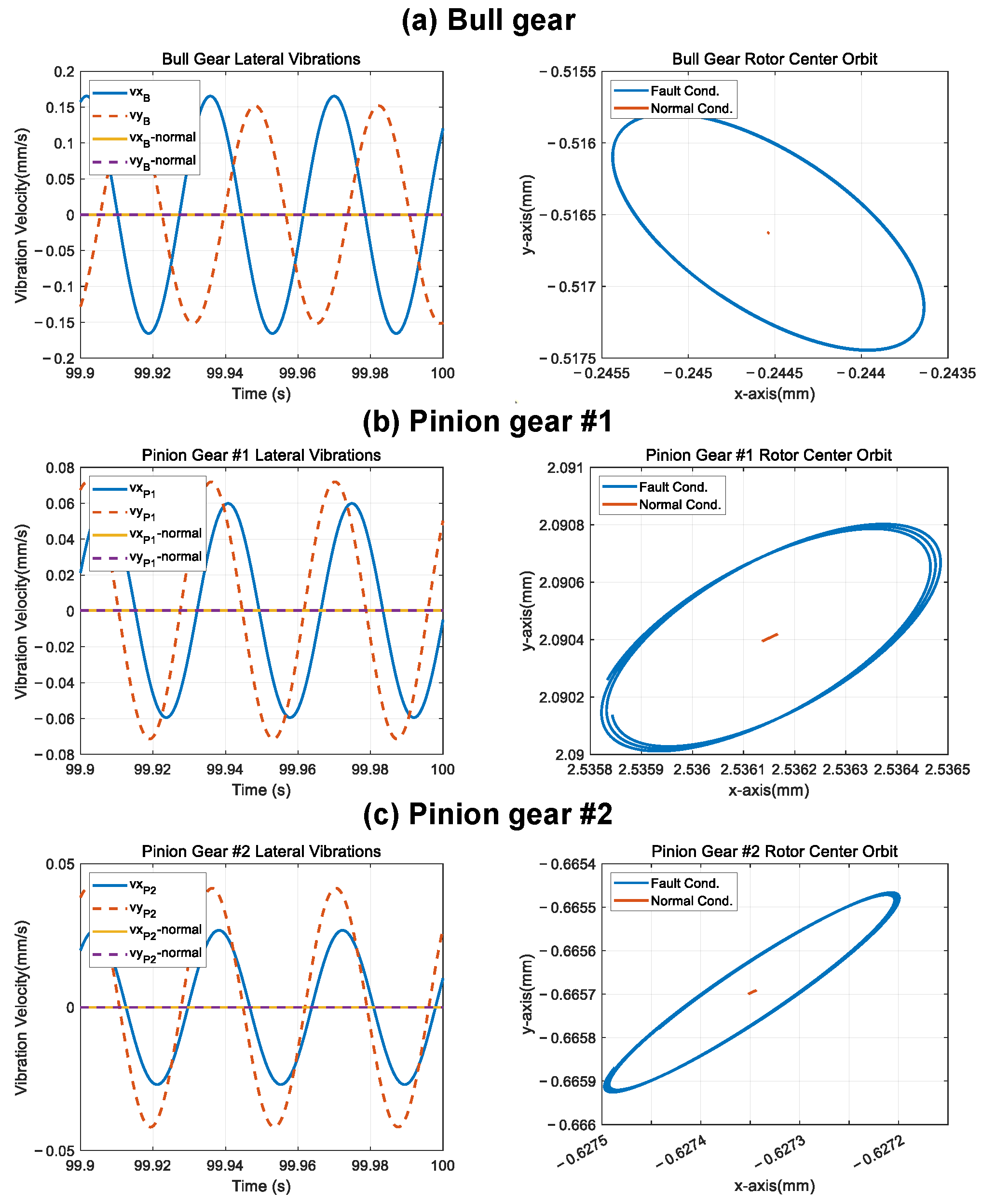
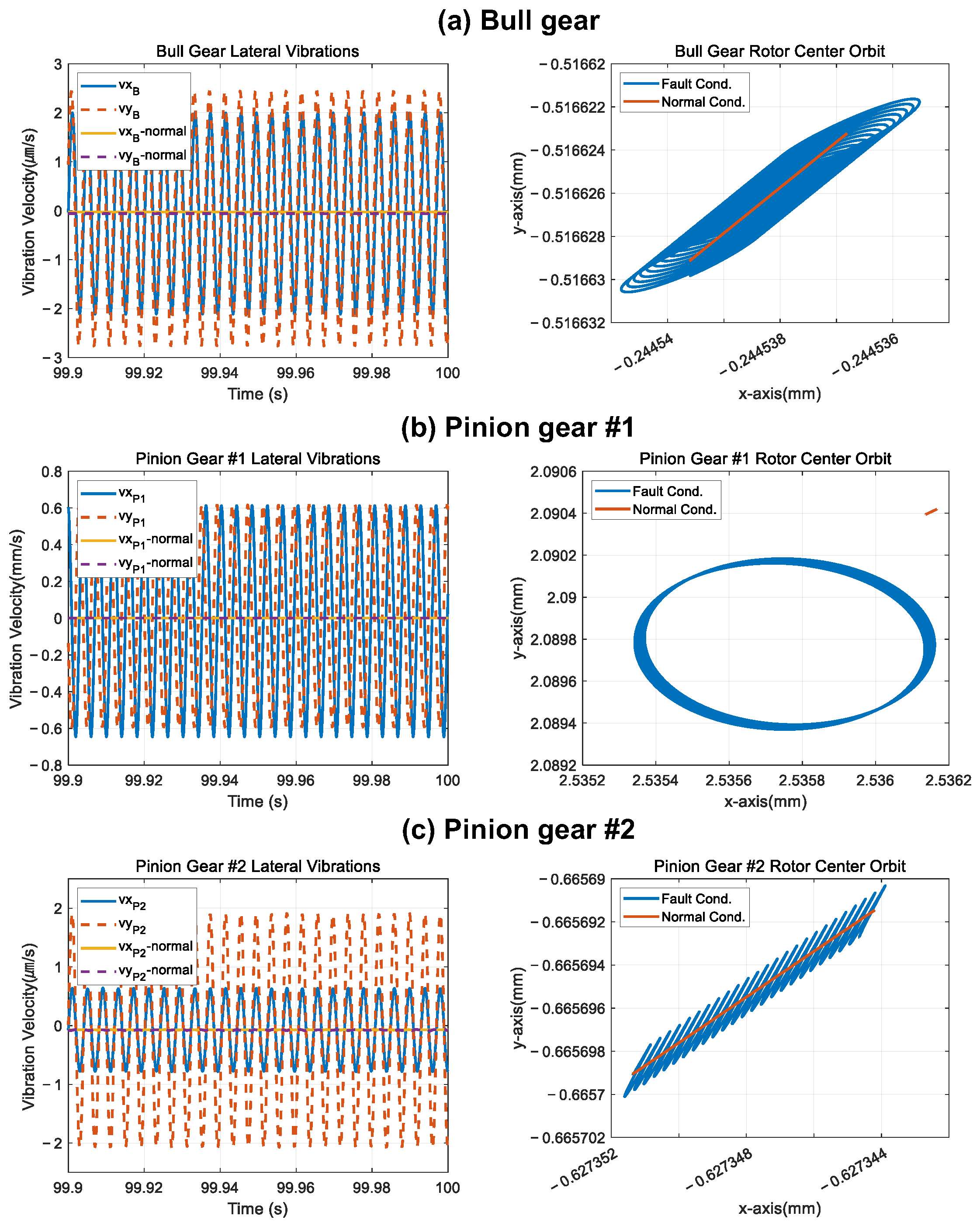
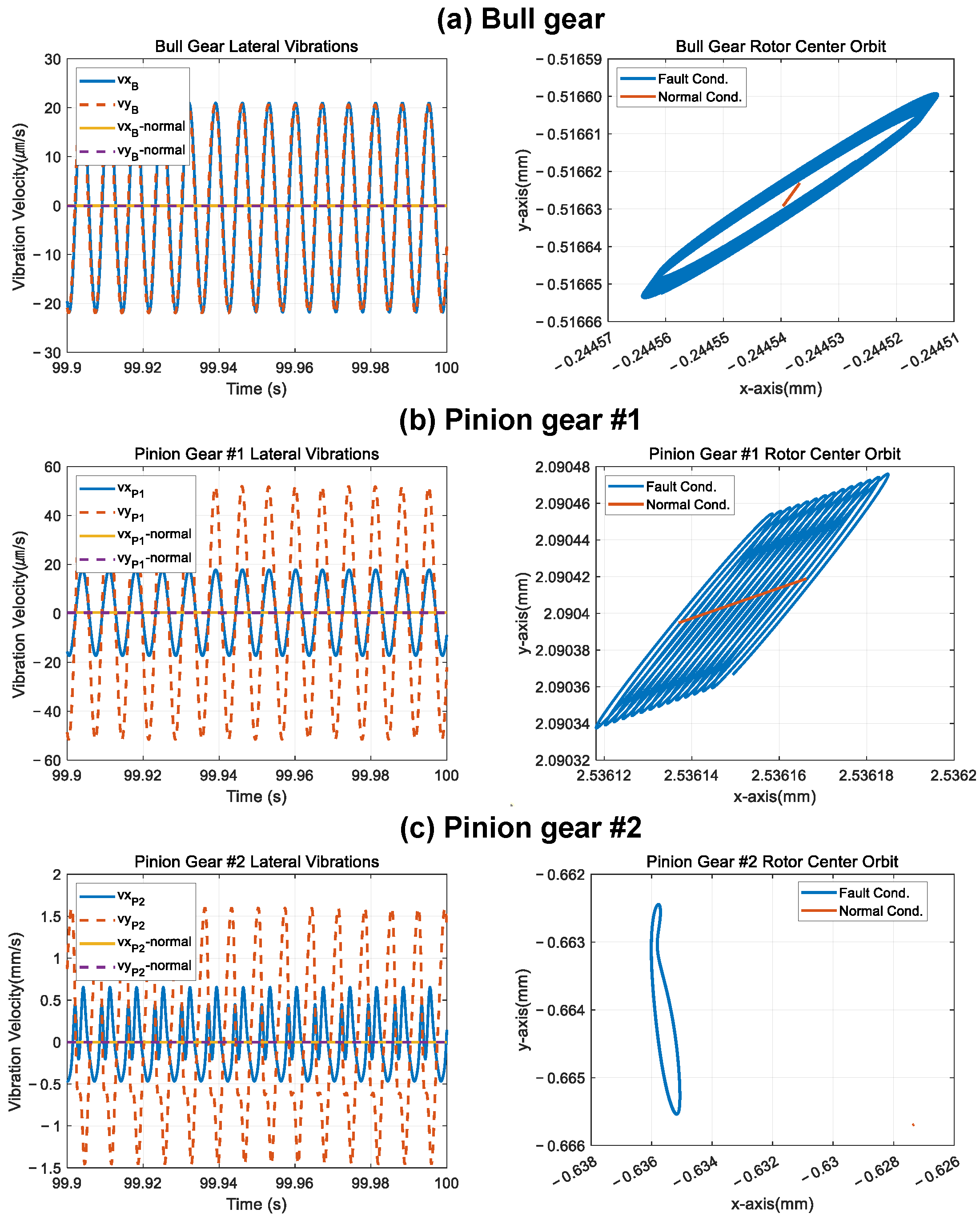
Figure 8, Figure 9, and Figure 10 show the lateral vibration analysis results and the shaft-centered orbits of Case 1, Case 2, and Case 3, respectively, compared with the normal condition. In the case of Case 1, it can be confirmed that the vibration of the main shaft with imbalance is the largest. Moreover, due to the characteristics of the fluid bearing in which the stiffness of the x-axis and y-axis are different, the shape of the orbit is elliptical. Compared to the normal condition, the elliptical diameter of the orbit in the defective condition is noticeably larger, and it can be confirmed through the orbit plot that the fault characteristics of the main shaft are transferred to the auxiliary shaft and change the orbit.
Rotor 2, which is connected to Rotor 1 by a gear, has a high rotational speed. Therefore, in the case of Case 2, the frequency due to the exciting force exists in a high range, so the vibration period is noticeably short in the vibration response. In addition, it can be confirmed that the orbits of the remaining two shafts draw an elliptical spiral with the same direction as the normal orbit. In the case of Case 2, as in Case 1, the vibration size of Rotor 2 with imbalance is the largest. In Case 3, the vibration of the shaft with imbalance is also the largest, and the fault of the auxiliary shaft induces the orbital changes in other shafts through the gear mesh.
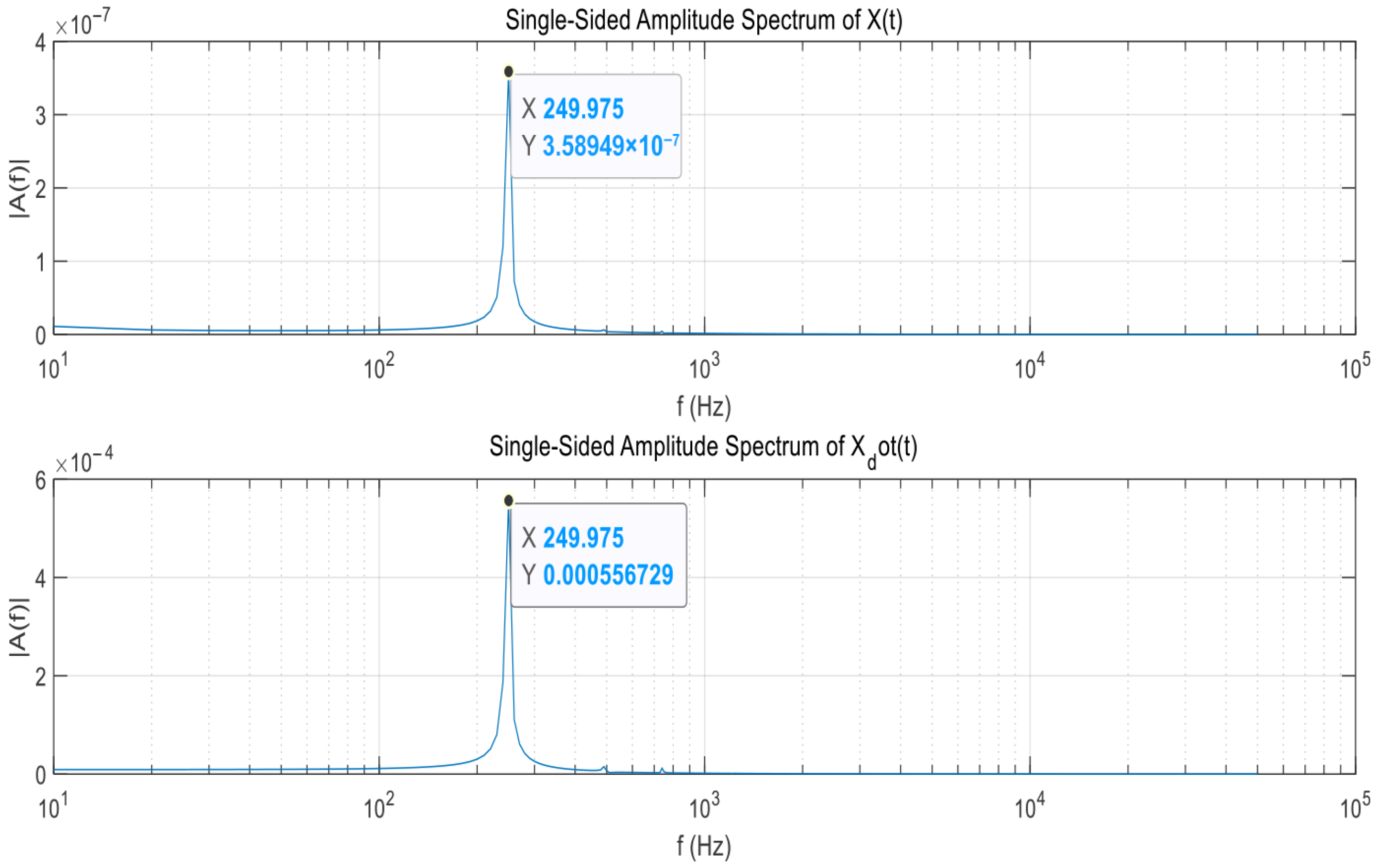
Figure 11, Figure 12, and Figure 13 are the results of FFT of the vibration displacement and vibration velocity of the time-series lateral vibration that occurred in Case 1, Case 2, and Case 3, respectively. In the case of Case 1, the magnitude of the exciting force due to the imbalance of the rotating machinery is proportional to the rotational speed, so it can be confirmed that it is amplified in the 1X component corresponding to the rotational speed frequency of 29.997 Hz in the FFT results.
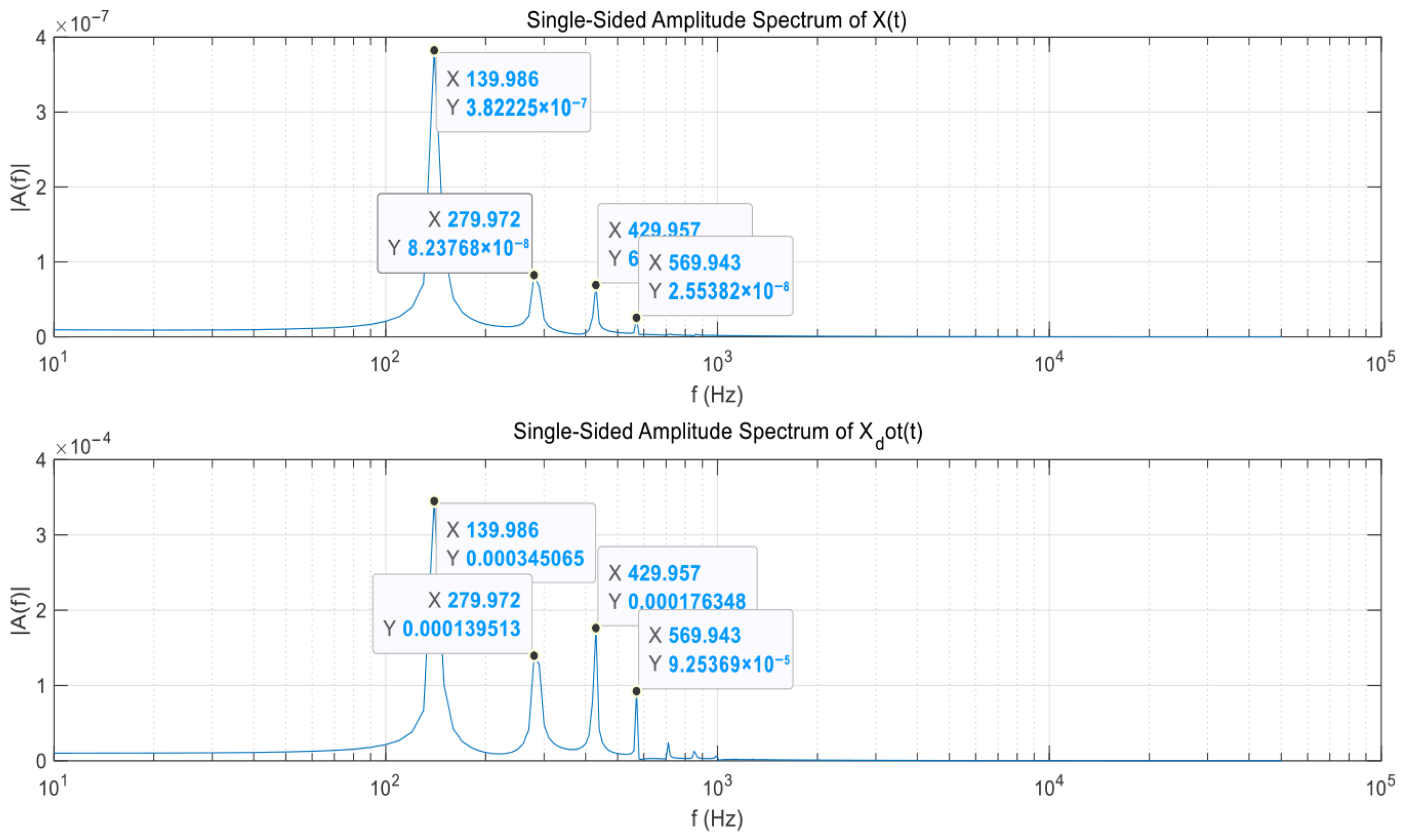
In the cases of Case 2 and Case 3, the rotational speed component of the shaft with imbalance acts as an exciting force, and the 1X component is amplified. In the FFT results of Case 3, it can be confirmed that other harmonic components occur simultaneously with the component corresponding to the rotational speed at 279.972 Hz. This is because the imbalance value of Rotor 3 is smaller than the imbalance value given to the other two shafts, so not only the direct synchronous component but also other frequency components are clearly observed.

5.2.2. Gear Teeth Fault Simulation

The reduction in the effective gear tooth width due to gear tooth damage reduces the rigidity of the gear meshing, which can be considered as a fault mode that changes the parameters of the model itself. The stiffness can be calculated by the following approximate equation using the ratio of the effective gear tooth width t b j (%) caused by damage to the main and pinion gears.
B u l l g e a r : k G M , B = 0.6817 · t b j 39.204 ( M N / m )
P i n i o n g e a r : k G M , P 1 = k G M , P 2 = 0.2224 · t b j + 6.8469 ( M N / m )
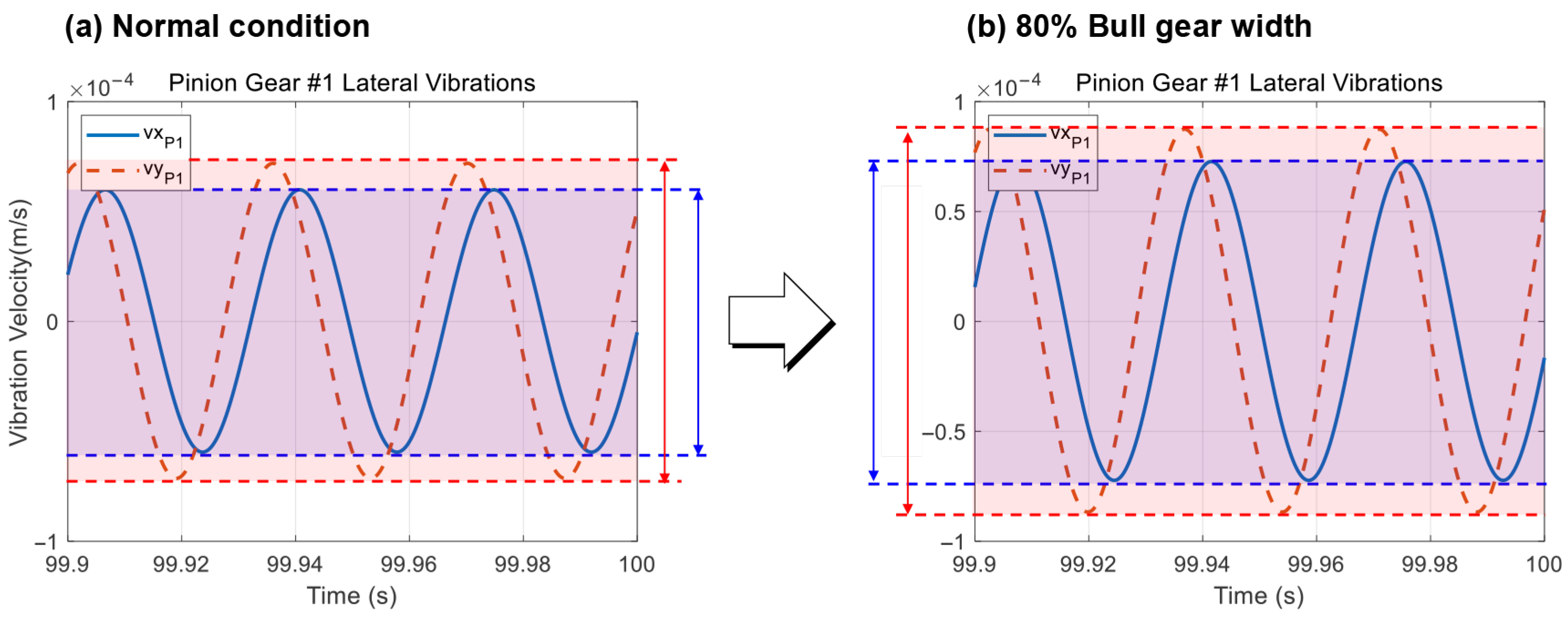
The gear teeth fault situation compared to the normal state is when the bull gear tooth width is reduced by 20%. The change in the model due to the reduction in gear-meshing stiffness reduces the natural frequency in the high-frequency range near 100 Hz, as shown in Figure 14. In addition, the time-series vibration response can cause an increase in amplitude, as shown in Figure 15, due to the reduction in gear-meshing stiffness.

6. Development of a Fault Simulator

6.1. Simulator Structure and Main Functions

The simulator is configured to allow users to intuitively set model parameters and fault conditions of a rotating system and to check the system response in real time. This provides a more intuitive and efficient analysis environment than the existing equation-based analysis and allows rapid simulation and evaluation of various faults.
The developed simulator is largely composed of four main functions as shown in Figure 16: model parameter setting, fault parameter setting, analysis condition setting, and simulation result visualization. First, the user inputs the dynamic characteristics of the main components of the system—shaft, gear, and bearing—by utilizing the model parameter adjustment function. Second, the user can set fault situations such as mass imbalance, gear damage, and bearing fault by using the fault simulation function and can easily apply different levels of faults. Once the state of the system is determined, the analysis conditions can be set by adjusting the simulation time range and sampling frequency through the analysis parameter setting function, and the rotational speed of the main shaft can be specified. When the analysis is completed through the simulation execution command, the user can check the time-series vibration response by utilizing the result visualization function. Here, the user can select the component whose response is to be displayed in the graph selection area and view the vibration velocity data for the torsional and lateral directions, as shown on the right. Through these functions, the user can intuitively analyze the fault characteristics of the rotating body system without complex equation analysis and clearly evaluate the impact of the fault on the system response.

6.2. Availability and Applications of GUI-Based Simulators

The simulator developed in this study can be utilized as a tool to overcome the difficulty of obtaining experimental data in fault diagnosis research and to quickly generate system responses reflecting various fault conditions. In addition, even when experimental data is insufficient, it can provide reliable fault data based on physical models, thereby improving the reliability of fault diagnosis and predictive maintenance (PHM) research. Figure 17 shows the various possible applications of the developed simulator.

6.2.1. Research on Machine Learning-Based Fault Diagnosis

In real systems, it is difficult to obtain data by simulating various fault conditions, and it takes a lot of money and time to obtain fault data through experiments. Using this simulator, various fault data such as imbalance, gear damage, and bearing faults can be quickly generated, and these datasets can be used as learning datasets for machine learning and data-based fault diagnosis models. Through this, the performance of fault diagnosis algorithms can be improved, and a more reliable fault detection system can be built.

6.2.2. Providing Reference Data for Building a Digital Twin System

Digital twin is a technology that monitors and predicts real-time conditions by linking real systems and virtual models and plays an important role in maintenance and fault prediction research. The data generated through the simulator developed in this study can be used as a standard for comparing and verifying the responses of the digital twin model and the real system, thereby improving the reliability of the digital twin model.

6.2.3. Comparison of Real System and Simulator Responses and Calibration of Model Performance

To verify the performance of the simulator and reflect more realistic system behavior, the accuracy of the model can be evaluated by comparing the responses of the simulator with actual experimental data. Through this comparative analysis, the parameters of the simulator can be adjusted to improve the model to a more sophisticated one.

7. Conclusions

In this paper, we present a physics-based vibration model of a rotating body that can be used to develop a condition diagnosis algorithm for rotating machinery. The proposed model is a lumped inertia-based model with a total of 20 DOF and reflects the characteristics of a multi-shaft system in which the lateral vibrations of each shaft influence each other as well as the coupling of lateral and torsional vibrations through a gear-meshing model. The model was converted into a state-space format, and a model reflecting the maximum torque of the motor and the aerodynamic load of the compressor and expander was input to build a simulation environment that simulates the situation in which the compander rotates at the required speed. Through the simulation, a time-series vibration response was generated, and the major fault situations of rotating machinery, such as mass imbalance and gear tooth damage, were simulated and compared with normal data. In addition, the behavior of the target system was analyzed based on the vibration response and orbital data.
This model can simulate faults such as bearing damage due to changes in the stiffness and damping values of the bearing in addition to mass imbalance, and impeller damage due to aerodynamic load and mass imbalance, so that it can be actively utilized in research for fault detection and diagnosis by acquiring time-series vibration responses for various fault modes. In addition, a GUI-based simulator using App Designer was developed so that users can intuitively adjust model and fault parameters and visually analyze the torsional and lateral vibration velocities of specific concentrated mass elements. Through this, reliable fault data can be generated quickly and its potential for use in various research fields related to fault diagnosis was explored.
However, the proposed model has limitations in that it is an ideal model that generates vibration signals only through physical interactions within the system, and realistic factors that have unexpected effects on equipment operation are not included. If the noise component of the signal is clearly identified based on actual operational data and incorporated as a disturbance into the proposed model, more realistic fault data can be generated. However, there is a practical limitation in that the operational data of the target equipment cannot be secured. Therefore, it is necessary to approximate some of the environmental noise by synthesizing mathematically defined AWGN (Additive White Gaussian Noise) and AR (Auto-Regressive) noise into the originally generated signal. In addition, the lack of actual operational data also serves as a limitation in the correlation between the model response and the operational data cannot be verified. To overcome this limitation, it is necessary to design a test bed that simulates the target system or to build a high-level digital twin model. An additional system capable of comparing the generated vibration response is expected to be used not only to verify the reliability of the proposed model but also to enable parallel improvement through mutual complementation.
Nevertheless, the physical model proposed in this study is significant in that it can precisely simulate the complex dynamic interaction of the shaft system that was not sufficiently reflected in previous studies by reflecting the coupling of each shaft, this simulating more realistic behavior. In addition, the state-space type simulator built based on the vibration model can quickly implement various faults of the rotating body with simple operations, effectively overcoming the difficulty of securing experimental data.
The proposed model can simulate not only the representative fault situations (imbalance and gear teeth fault) adopted in this study but also bearing faults and load faults. In addition, by incorporating the physical mechanisms of various fault conditions that occur in actual systems into the model, faults can be easily implemented. Through this approach, data on fault situations that are difficult to obtain from actual equipment can be rapidly generated and applied to machine learning-based fault diagnosis research, enabling the performance of fault detection algorithms to be verified and improved. In addition, generated data can be used as reference data for building a digital twin system, and comparison and verification with the actual system are possible through the system response data generated using the simulator. Furthermore, the performance of the simulator can be continuously corrected through comparison with the experimental data, and it can be developed into a model that can reflect realistic system behavior.
The state-space-based multi-shaft rotating body simulator proposed in this study can contribute to increasing the reliability of fault detection and diagnosis research, and it is expected that it can be utilized in the state diagnosis and predictive maintenance research of various rotating machineries in the future.

Author Contributions

S.H.K.: conceptualization, methodology, validation, investigation, writing; H.M.S.: validation, investigation; S.H.J.: methodology, writing; W.J.L.: investigation, methodology; S.J.K.: methodology, validation, investigation, writing, supervision, project administration. All authors have read and agreed to the published version of the manuscript.

Funding

This work was supported by the Korea Research Institute for Defense Technology Planning and Advancement (KRIT)—grant funded by the Defense Acquisition Program Administration (DAPA) (KRIT-CT-22-081, Weapon System CBM+ Research Center). It was also partly supported by the National Research Foundation of Korea (NRF)—grant funded by the Government of South Korea (MSIT) (No. RS-2025-00555918).

Data Availability Statement

Data is unavailable due to privacy.

Conflicts of Interest

Author Won Joon Leewas employed by the company Hanwha Ocean Co., Ltd. The remaining authors declare that the research was conducted in the absence of any commercial or financial relationships that could be construed as a potential conflict of interest.

Abbreviations

The following abbreviations are used in this manuscript:
DOFDegrees of Freedom
MBull
BgearMotor
P1Pinion gear #1
P2Pinion gear #2
St1Stage#1
St2Stage#2
St3Stage#3
ExpExpander
lRefers to lateral vibration components
tRefers to torsional vibration components
x1, x2Position identifiers along the X-direction
y1, y2Position identifiers along the Y-direction
x1y1, x2y2Cross-coupled term between X and Y direction
rImbalanced rotor
θ Torsional angular displacement
ω Angular velocity
t Time
Q n Non-conservative force
[ J ] Torsional Inertia Matrix
C Damping Matrix
[ K ] Stiffness Matrix
g Gear teeth ratio, i = 1,2
r Gear teeth
J Torsional Inertia
k Stiffness
c Damping
c T Total equivalent damping coefficient
B t Hydrodynamic damping coefficient
m Mass
x yLateral displacement in x, y direction
α , β Angular displacement
I T Moment of inertia
I P Polar moment of inertia
a , b Distance from the center of the disk
φ Pressure Angle
W j Tooth Width
t a j Tooth Thickness at Addendum Circle
h a j Tooth Height at Addendum Circle
h c j Tooth Height at Center
h b j Tooth Height at Dedendum Circle
t b j Tooth Thickness at Dedendum Circle
ω j Tooth profile slope coefficient
ν Poisson ratio
F n Normal tooth contact force
E Young’s modulus
G Shear modulus
f Gear mesh frequency
k j Gear mesh stiffness
δ b p j Deflection due to bending deformation induced by horizontal contact force
δ b n j Deflection due to bending deformation induced by vertical contact force
δ s j Deformation induced by shear force
δ f j Deflection due to the bending of gear teeth
δ h j Deformation due to compressive contact at the meshing surface
k h Gear mesh stiffness in the normal direction
u i g Transitional displacement of gear I along x-direction, i = 1,2
v i g Transitional displacement of gear I along y-direction, i = 1,2
θ i g Rotational displacement of gear, i = 1,2
r i Pitch radius of gear, i = 1,2
F h x B i , F h y B i Gear mesh force components (X and Y directions) transmitted from pinion i to bull gear B, i = 1,2
T B i Torque applied to the bull gear shaft B via connection with pinion i, i = 1,2
T P i Reaction torque acting on pinion gear i from load or gear mesh, i = 1,2
X State vector
U Input vector
Y Output vector
A , B , C , D State-space matrices
F r 1 , x , F r 1 , y Imbalanced-induced excitation force
k G M , i Gear stiffness with respect to face width variation, i = B, P1, P2

References

  1. Lu, K.; Jin, Y.; Chen, Y.; Yang, Y.; Hou, L.; Zhang, Z.; Li, Z.; Fu, C. Review for order reduction based on proper orthogonal decomposition and outlooks of applications in mechanical systems. Mech. Syst. Signal Process. 2019, 123, 264–297. [Google Scholar] [CrossRef]
  2. Wei, Y.; Li, Y.; Xu, M.; Huang, W. A review of early fault diagnosis approaches and their applications in rotating machinery. Entropy 2019, 21, 409. [Google Scholar] [CrossRef] [PubMed]
  3. Lie, C.H.; Chun, Y.H. An algorithm for preventive maintenance policy. IEEE Trans. Reliab. 2007, 35, 71–75. [Google Scholar] [CrossRef]
  4. Guillén, A.J.; Crespo, A.; Gómez, J.F.; Sanz, M.D. A framework for effective management of condition based maintenance programs in the context of industrial development of E-Maintenance strategies. Comput. Ind. 2016, 82, 170–185. [Google Scholar] [CrossRef]
  5. An, D.; Kim, N.H.; Choi, J.H. Practical options for selecting data-driven or physics-based prognostics algorithms with reviews. Reliab. Eng. Syst. Saf. 2015, 133, 223–236. [Google Scholar] [CrossRef]
  6. Luo, J.; Bixby, A.; Pattipati, K.; Qiao, L.; Kawamoto, M.; Chigusa, S. An Interacting Multiple Model Approach to Model-Based Prognostics. In Proceedings of the 2003 IEEE International Conference on Systems, Man and Cybernetics (SMC’03), Washington, DC, USA, 5–8 October 2003. [Google Scholar]
  7. Chen, Z.; Li, W. Multisensor feature fusion for bearing fault diagnosis using sparse autoencoder and deep belief network. IEEE Trans. Instrum. Meas. 2017, 66, 1693–1702. [Google Scholar] [CrossRef]
  8. Sawalhi, N.; Ganeriwala, S.; Tóth, M. Parallel misalignment modeling and coupling bending stiffness measurement of a rotor-bearing system. Appl. Acoust. 2019, 144, 124–141. [Google Scholar] [CrossRef]
  9. Ignjatovska, A.; Pandilov, Z.; Petreski, Z. Physics-Based, Data-Driven, and Physics-Based Data-Driven Methods for Diagnostics of Rotating Machinery-State of the Art. Ann. Fac. Eng. Hunedoara. 2023, 21, 43–52. [Google Scholar]
  10. Aykol, M.; Gopal, C.B.; Anapolsky, A.; Herring, P.K.; van Vlijmen, B.; Berliner, M.D.; Bazant, M.Z.; Braatz, R.D.; Chueh, W.C.; Storey, B.D. Perspective—Combining physics and machine learning to predict battery lifetime. J. Electrochem. Soc. 2021, 168, 030525. [Google Scholar] [CrossRef]
  11. Khorasgani, H.; Farahat, A.; Ristovski, K.; Gupta, C.; Biswas, G.A. Framework for Unifying Model-Based and Data-Driven Fault Diagnosis. In Proceedings of the 2018 Annual Conference of the Prognostics and Health Management Society, Philadelphia, PA, USA, 24–27 September 2018. [Google Scholar]
  12. Atoui, M.A.; Cohen, A. Coupling data-driven and model-based methods to improve fault diagnosis. Comput. Ind. 2021, 128, 103401. [Google Scholar] [CrossRef]
  13. Kannan, P.; Neha, S. Ball Bearing Fault by Feature Extraction and Fault Diagnosis Method Based on AI ML Algorithms. In Proceedings of the 2022 6th International Conference on Intelligent Computing and Control Systems (ICICCS), Madurai, India, 25–27 May 2022. [Google Scholar] [CrossRef]
  14. Hemalatha, S.; Kavitha, T.; Anand, P. Effectiveness of Classification Techniques for Fault Bearing Prediction. In Proceedings of the 2022 6th International Conference on Electronics, Communication and Aerospace Technology (ICECA), Coimbatore, Tamil Nadu, India, 1–3 December 2022. [Google Scholar] [CrossRef]
  15. Lang, W.; Hu, Y.; Gong, C.; Zhang, X.; Xu, H.; Deng, J. Artificial intelligence-based technique for fault detection and diagnosis of EV motors: A review. IEEE Trans. Transp. Electrif. 2021, 8, 384–406. [Google Scholar] [CrossRef]
  16. Hasan, A.; Singh, J. Fault Detection in Ball Bearing through Machine Learning Models. In Proceedings of the 2022 6th International Conference on Electronics, Communication and Aerospace Technology (ICECA), Coimbatore, Tamil Nadu, India, 1–3 December 2022. [Google Scholar] [CrossRef]
  17. Ding, Y.; Jia, M.; Miao, Q.; Cao, Y. A novel time–frequency Transformer based on self–attention mechanism and its application in fault diagnosis of rolling bearings. Mech. Syst. Signal Process. 2022, 168, 108616. [Google Scholar] [CrossRef]
  18. Kumar, S. Intelligent Bearing Fault Diagnosis and Classification Based on Support Vector Machine. In Proceedings of the 2021 2nd Global Conference for Advancement in Technology (GCAT), Bangalore, India, 1–2 October 2021. [Google Scholar] [CrossRef]
  19. Ji, D.; Hu, M.; Wang, M. Research on the Motor Fault Diagnosis Method Based on Feature Engineering and Machine Learning. In Proceedings of the 2022 7th International Conference on Intelligent Computing and Signal Processing (ICSP), Xi’an, China, 16 April 2022. [Google Scholar] [CrossRef]
  20. Yuan, L.; Lian, D.; Kang, X.; Chen, Y.; Zhai, K. Rolling Bearing Fault Diagnosis Based on Convolutional Neural Network and Support Vector Machine. IEEE Access 2020, 8, 137395–137406. [Google Scholar] [CrossRef]
  21. Guo, J.; Liu, X.; Li, S.; Wang, Z. Bearing intelligent fault diagnosis based on wavelet transform and convolutional neural network. Shock Vib. 2020, 2020, 6380486. [Google Scholar] [CrossRef]
  22. Sacerdoti, D.; Strozzi, M.; Secchi, C. A comparison of signal analysis techniques for the diagnostics of the IMS rolling element bearing dataset. Appl. Sci. 2023, 13, 5977. [Google Scholar] [CrossRef]
  23. Eren, L.; Ince, T.; Kiranyaz, S. A generic intelligent bearing fault diagnosis system using compact adaptive 1D CNN classifier. J. Signal Process. Syst. 2019, 91, 179–189. [Google Scholar] [CrossRef]
  24. Kavianpour, M.; Ghorvei, M.; Kavianpour, P.; Ramezani, A.; Beheshti, M.T. An Intelligent Gearbox Fault Diagnosis under Different Operating Conditions Using Adversarial Domain Adaptation. In Proceedings of the 2022 8th International Conference on Control, Instrumentation and Automation (ICCIA), Tehran, Iran, 2–3 March 202.
  25. Zhu, X.; Yang, D.; Pan, H.; Karimi, H.R.; Ozevin, D.; Cetin, A.E. A novel asymmetrical autoencoder with a sparsifying discrete cosine stockwell transform layer for gearbox sensor data compression. Eng. Appl. Artif. Intel. 2024, 127, 107322. [Google Scholar] [CrossRef]
  26. Hejazi, S.Z.; Packianather, M.; Liu, Y. A novel customised load adaptive framework for induction motor fault classification utilising MFPT bearing dataset. Machines 2024, 12, 44. [Google Scholar] [CrossRef]
  27. Mohiuddin, M.; Islam, M.S. Rolling element bearing faults detection and classification technique using vibration signals. Eng. Proc. 2022, 27, 53. [Google Scholar] [CrossRef]
  28. Sadoughi, M.; Hu, C. A Physics-Based Deep Learning Approach for Fault Diagnosis of Rotating Machinery. In Proceedings of the IECON 2018–44th Annual Conference of the IEEE Industrial Electronics Society, Washington, DC, USA, 21–23 October 2018. [Google Scholar] [CrossRef]
  29. Li, W.; Zhu, Z.; Jiang, F.; Zhou, G.; Chen, G. Fault diagnosis of rotating machinery with a novel statistical feature extraction and evaluation method. Mech. Syst. Signal Process. 2015, 50–51, 414–426. [Google Scholar] [CrossRef]
  30. Qin, H.Q.; Si, X.S.; Lv, Y.R. Feature Denoising-Based Fault Diagnosis for Rotating Machinery. In Proceedings of the 2020 35th Youth Academic Annual Conference of Chinese Association of Automation (YAC), Zhanjiang, China, 16–18 October 2020. [Google Scholar] [CrossRef]
  31. Liu, J.; Zhou, K.; Yang, C.; Lu, G. Imbalanced fault diagnosis of rotating machinery using autoencoder-based SuperGraph feature learning. Front. Mech. Eng. 2021, 16, 829–839. [Google Scholar] [CrossRef]
  32. Yamamoto, G.K.; da Costa, C.; da Silva Sousa, J.S. A smart experimental setup for vibration measurement and imbalance fault detection in rotating machinery. Case Stud. Mech. Syst. Signal Process. 2016, 4, 8–18. [Google Scholar] [CrossRef]
  33. Hanachi, H.; Liu, J.; Banerjee, A.; Chen, Y.; Koul, A. A physics-based modeling approach for performance monitoring in gas turbine engines. IEEE Trans. Reliab. 2014, 64, 197–205. [Google Scholar] [CrossRef]
  34. Gálvez, A.; Diez-Olivan, A.; Seneviratne, D.; Galar, D. Fault detection and RUL estimation for railway HVAC systems using a hybrid model-based approach. Sustainability 2021, 13, 6828. [Google Scholar] [CrossRef]
  35. Chen, G. A new rotor-ball bearing-stator coupling dynamics model for whole aero-engine vibration. J. Vib. Acoust. 2009, 131, 061009. [Google Scholar] [CrossRef]
  36. Wang, J.G.; Chen, X.; Bi, X.; Luo, Z.; Mo, R. Dynamic analysis of TBM multi-gear parallel transmission system considering the influence of multiple factors. J. Mech. Sci. Technol. 2024, 38, 5323–5340. [Google Scholar] [CrossRef]
  37. Qin, Y.; Liu, H.; Mao, Y. Faulty rolling bearing digital twin model and its application in fault diagnosis with imbalanced samples. Adv. Eng. Inform. 2024, 61, 102513. [Google Scholar] [CrossRef]
  38. Xia, J.; Huang, R.; Liao, Y.; Li, J.; Chen, Z.; Li, W. Digital twin-assisted gearbox dynamic model updating toward fault diagnosis. Front. Mech. Eng. 2023, 18, 32. [Google Scholar] [CrossRef]
  39. Xia, M.; Shao, H.; Williams, D.; Lu, S.; Shu, L.; de Silva, C.W. Intelligent fault diagnosis of machinery using digital twin-assisted deep transfer learning. Reliab. Eng. Syst. Saf. 2023, 215, 107938. [Google Scholar] [CrossRef]
  40. Singh, D.S.; Agrawal, A.; Mahapatra, D.R. A reduced-order modeling framework for simulating signatures of faults in a bladed disk. arXiv 2021, arXiv:2108.06265. [Google Scholar] [CrossRef]
  41. Mohammadabadi, S.M.S.; Entezami, M.; Moghaddam, A.K.; Orangian, M.; Nejadshamsi, S. Generative artificial intelligence for distributed learning to enhance smart grid communication. Int. J. Intell. Netw. 2024, 5, 267–274. [Google Scholar] [CrossRef]
  42. Nejadshamsi, S.; Bentahar, J.; Eicker, U.; Wang, C.; Jamshidi, F. A geographic-semantic context-aware urban commuting flow prediction model using graph neural network. Expert Syst. Appl. 2025, 261, 125534. [Google Scholar] [CrossRef]
  43. Dimopoulos, G.; Frangopoulos, C. A dynamic model for liquefied natural gas evaporation during marine transportation. Int. J. Thermodyn. 2008, 11, 123–131. [Google Scholar]
  44. Oh, C.; Song, Y.U. A Study on the Improvement of LNGC Re-liquefaction System. J. Navig. Port. Res. 2009, 33, 659–664. [Google Scholar] [CrossRef]
  45. Ma, H.; Pang, X.; Zeng, J.; Wang, Q.; Wen, B. Effects of gear crack propagation paths on vibration responses of the perforated gear system. Mech. Syst. Signal Process. 2015, 62, 113–128. [Google Scholar] [CrossRef]
  46. Werner, U. Mathematical rotordynamic model regarding excitation due to elliptical shaft journals in electrical motors considering the gyroscopic effect. Appl. Math. 2013, 4, 57–74. [Google Scholar] [CrossRef]
  47. Ishibashi, T.; Kawai, T. Modelling of Oil Film Bearings. In Proceedings of the 2nd Japanese Modelica Conference, Tokyo, Japan, 17–18 May 2018. [Google Scholar] [CrossRef]
  48. Nicholas, J.C.; Gunter, E.J.; Allaire, P.E. Stiffness and damping coefficients for the five-pad tilting-pad bearing. ASLE Trans. 1979, 22, 113–124. [Google Scholar] [CrossRef]
  49. Kim, C.S.; Kim, S.T.; Cho, S.Y.; Jung, H.H. The Effect of Gear Contact Stiffnesses on the Vibration of Torsional Geared Systems for a Mill Turret. J. Korean Soc. Manuf. Process. Eng. 2009, 8, 32–39. [Google Scholar]
  50. Kim, S.J.; Kim, Y.R.; Min, S. Study of Gas-turbine Cranking Model using the Coast Down Experimental Results. J. Korean Soc. Propuls. Eng. 2017, 21, 18–24. [Google Scholar] [CrossRef]
  51. Edwards, S.; Lees, A.W.; Friswell, M.I. Fault diagnosis of rotating machinery. Shock Vib. Dig. 1998, 30, 4–13. [Google Scholar]
  52. Wang, B.; Xu, Y.; Wang, M.; Li, Y. Gear fault diagnosis method based on the optimized graph neural networks. IEEE Trans. Instrum. Meas. 2023, 73, 1–11. [Google Scholar] [CrossRef]
  53. ISO21940-11:2016; Mechanical Vibration-Rotor Balancing-Part 11: Procedures and Tolerances for Rotors with Rigid Behaviour. ISO: Geneva, Switzerland, 2016.
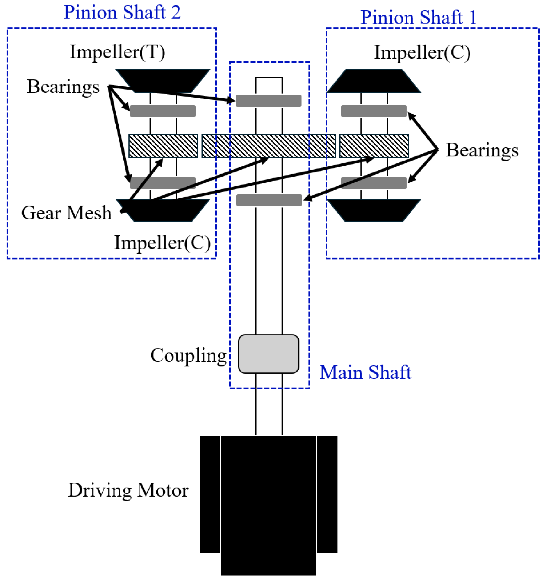
Figure 1. Physical layout of the re-liquefaction system.
Jmse 13 01321 g001
Figure 2. Torsional vibration model of LNG re-liquefaction system.
Jmse 13 01321 g002
Figure 3. Lumped inertia based lateral model.
Jmse 13 01321 g003
Figure 4. Shaft classification for the lateral model.
Jmse 13 01321 g004
Figure 5. Geometry and parameters of gear teeth.
Jmse 13 01321 g005
Figure 6. Aerodynamic load of each stage according to rotational speed.
Jmse 13 01321 g006
Figure 7. Simulator implemented in MATLAB/Simulink environment.
Jmse 13 01321 g007
Figure 8. Simulation results of Case 1.
Jmse 13 01321 g008
Figure 9. Simulation results of Case 2.
Jmse 13 01321 g009
Figure 10. Simulation result of Case 3.
Jmse 13 01321 g010
Figure 11. FFT result of Case 1.
Jmse 13 01321 g011
Figure 12. FFT result of Case 2.
Jmse 13 01321 g012
Figure 13. FFT result of Case 3.
Jmse 13 01321 g013
Figure 14. Change in natural frequency (highlighted in yellow color) due to reduction in gear-meshing stiffness: (a) normal, (b) bull gear width reduced by 20%.
Jmse 13 01321 g014
Figure 15. Changes in vibration response due to reduction in gear-meshing stiffness: (a) normal, (b) bull gear width reduced by 20%.
Jmse 13 01321 g015
Figure 16. Architecture and functions of the simulator.
Jmse 13 01321 g016
Figure 17. Applications of the GUI-based simulator.
Jmse 13 01321 g017
Table 1. Dimensional stiffness and damping values of sleeve bearings.
k x x k x y k y x k y y c x x c x y c y x c y y
1.0244 × 1081.4384 × 107−2.0332 × 1082.6898 × 1085.8084 × 105−5.5866 × 10⁵−5.5866 × 1051.7420 × 106
Table 2. Dimensional stiffness and damping values of tilting pad bearings.
k x x k x y k y x k y y c x x c x y c y x c y y
#12.40 × 106008.00 × 1061.51 × 104002.02 × 104
#22.16 × 106007.20 × 1061.36 × 104001.82 × 104
#31.96 × 106006.54 × 1061.08 × 104001.43 × 104
#41.54 × 106003.36 × 1061.38 × 104001.54 × 104
Table 3. Imbalance amount of each shaft.
Simulation Case Number Imbalance Position Imbalance Amount (kg∙m)
Case 1Rotor 1(R1)0.006378
Case 2Rotor 2(R2) Pinion#15.56 × 10⁻⁵
Case 3Rotor 3(R3) Pinion#22.63 × 10⁻⁵
Disclaimer/Publisher’s Note: The statements, opinions and data contained in all publications are solely those of the individual author(s) and contributor(s) and not of MDPI and/or the editor(s). MDPI and/or the editor(s) disclaim responsibility for any injury to people or property resulting from any ideas, methods, instructions or products referred to in the content.