Acoustic Analysis of Fish Tanks for Marine Bioacoustics Research

Abstract

Underwater sounds play a key role in biodiversity as many marine animals use these to know their environment and to communicate among themselves. Unfortunately, anthropogenic noise makes this communication more difficult due to masking effects and may also produce harmful effects that compromise their preservation and survival. Many researchers have studied the influence of underwater noise on marine species in laboratory conditions using fish tanks. Consequently, studying the acoustic response of these fish tanks constitutes an essential task to better understand the results obtained in those experiments. In this work, a theoretical model and acoustic measurements were used to assess the uncertainty of a fish tank setup. The proposed methodology aims to improve the effectiveness of those studies involving fish tanks by an in-depth analysis of the sound field spatial distribution. Preliminary results show that this distribution depends on the frequency of the generated sound, the water level, and the measurement depth thus confirming the importance of analyzing the range of applicability of these setups.

1. Introduction

Many marine species are impacted negatively by human activities resulting in anthropogenic noise in the underwater environment [1]. This noise can significantly affect the fish population, pushing them to migrate from their favorable environment, making their successful reproduction difficult, or compromising survival [2]. Some examples of anthropogenic noise sources are fishing boats, transportation and trading vessels, offshore wind turbines, activities associated with oil and gas prospection, and many more [3]. Several studies have been carried out to study the effect of anthropogenic noise on marine species in deep water [4], shallow water [5], aquaculture facilities [6], or fish tanks [7]. Results revealed the differences in the acoustic field depending on the scenario. While deep water environments resemble acoustic free-field conditions, the remaining scenarios yield a diffuse field due to the multiple reflections in the seabed or boundary surfaces. In this context, the study of the acoustic field in fish tanks is of great interest in the science of bioacoustics to examine the behavior of marine species in response to different sound stimuli in a much more controlled environment [8].

The acoustic field in semi-closed spaces as in the case of fish tanks depends on their dimensions and consequently on the frequency under analysis [9]. In this regard, knowing the spatial distribution of this sound field allows properly evaluating the effect that anthropogenic noise has on the behavior of these species, thus contributing, first to the standardization of scientific methods and secondly, to the adoption of measures that guarantee their well-being such as the development of metrics for regulating exposure [10]. Moreover, given that the anthropogenic noise sources found in the marine environments have different frequency spectra, it is of great importance to explore the dependence of the sound field spatial distribution on the frequency of analysis. Some authors have illustrated these phenomena by using theoretical approaches based on the finite element method [11,12] or the finite difference method [13], the analytical approach proposed by Novak et al. [14] being of great interest because it accounts for the leakage through the walls of the tank. To the author’s knowledge, most of the laboratory studies found in the literature do not account for the above issues, which may result in misleading conclusions about the behavior of the marine species [15] and prevent comparison between results. Therefore, analyzing the acoustics of fish tanks is of great importance not only to better understand the behavior of marine species subjected to noise [16] but also in the design and development of solutions that reduce it in the above environments [17].

The main aim of this work is to study the spatial sound field distribution in fish tanks using a theoretical model and by performing laboratory experiments in a water-filled fish tank. For this purpose, the analytical model proposed by Novak et al. was first implemented, and an experimental setup was prepared to measure the sound field in horizontal planes in a fish tank using a robotized system. The normal modes of vibration (i.e., frequencies of maximum sound level in the water fluid of the fish tank) were first calculated and compared to those obtained in the experiments, with results showing the differences in the sound field spatial distribution for each mode. Next, an in-depth analysis of the influence of the water level, the measurement depth, and the sound source level on the frequency spectrum was performed, with results showing the sound level dependence on these factors. Finally, a discussion on the low-frequency acoustic behavior of fish tanks, together with some remarks on the potential possibilities of the proposed methodology to come up with the most appropriate fish tank arrangement for bioacoustics experiments, was given.

From the above tasks, the following specific objectives can be outlined:

▪

Determination of the acoustic normal modes of a water-filled fish tank both theoretically and experimentally.

▪

Analysis of the sound field spatial distribution for these frequencies over horizontal planes at different depths.

▪

Study of the influence of modifying the water level and the sound source intensity on the sound pressure level frequency spectrum.

▪

Perform a preliminary exploration of the vibroacoustic behavior and the uncertainty in the low-frequency analysis of fish tanks.

This paper is organized as follows. Section 2 introduces the background theory related to fish tanks in bioacoustics and the study of the sound field in water-filled fish tanks. In Section 3, the fish tank and the measurement system used for the experiments are described in detail along with a review of the prediction model proposed by Novak et al. [14]. In Section 4, experimental results for normal modes and spatial sound field distribution are analyzed and compared to those obtained using the prediction model. In addition, a discussion on the influence of parameters such as the water level, the measurement depth, and the sound source power was carried out, and some remarks were given to highlight the potential of the proposed methodology. Finally, Section 5 summarizes the main conclusions of this work.

2. Background Theory

2.1. Importance of Fish Tanks in Bioacoustics

In bioacoustics, many laboratory experiments related to the study of the impact of anthropogenic noise on marine species are performed in water tanks, waveguides, or small pools [8]. Among these, water tanks can be classified by size according to their dimensions and the wavelength of the sound signal used for the experiments, small aquaria being commonly referred to as fish tanks. In general, the study of the sound field in a water-filled tank usually requires measuring the acoustic pressure when a sound wave is generated inside it. These measurements involve underwater transducers to be used as sound sources and hydrophones (i.e., acoustic pressure sensors). However, given that fish are normally free to move in a fish tank, the sound level to which fish are exposed can differ depending on their position. Under such conditions, knowing the sound field distribution in such spaces constitutes a key point for a better understanding of fish’s behavior when a sound is produced inside it. Therefore, this issue should be taken into consideration by researchers in bioacoustics in the choice of fish tanks and the preparation of the experimental setups for their studies.

2.2. Sound Field in Water-Filled Rectangular Tanks

In the case of small tanks of simple shape, such as rectangular ones, the sound field inside the fish tank can be analyzed using simple formulas under the assumption of rigid walls. In doing so, the acoustic response may be approximated using a zero-order approximation (i.e., Dirichlet boundary conditions) [9]. In brief, the sound field inside the enclosure is described as the combination of the sound radiated from the source and the multiple reflections in its walls and top surface, yielding a reverberant field [18]. This superposition effect gives rise to the so-called normal frequencies or normal modes of vibration, which correspond to those frequencies at which the Sound Pressure Level (SPL) in the water of the fish tank reaches very high values. Nevertheless, this is not strictly true in practice because the damping effect of the fish tank surfaces absorbs part of the acoustic energy. Consequently, not only the normal modes but also the sound pressure spatial distribution will be changed from that for the rigid-walls case. Novak et al. [14] proposed an analytical model to describe the sound field in thin-walled rectangular tanks accounting for this damping effect by using a modal summation approach. Their approximate model was shown to be suited to predict the acoustic field in these tanks. Alternatively, numerical models based on the finite element method or the finite difference method as those proposed by Rogers et al. [11] and Duncan et al. [13], respectively, can be adopted in the case of irregularly shaped tanks or more complex geometries.

3. Materials and Methods

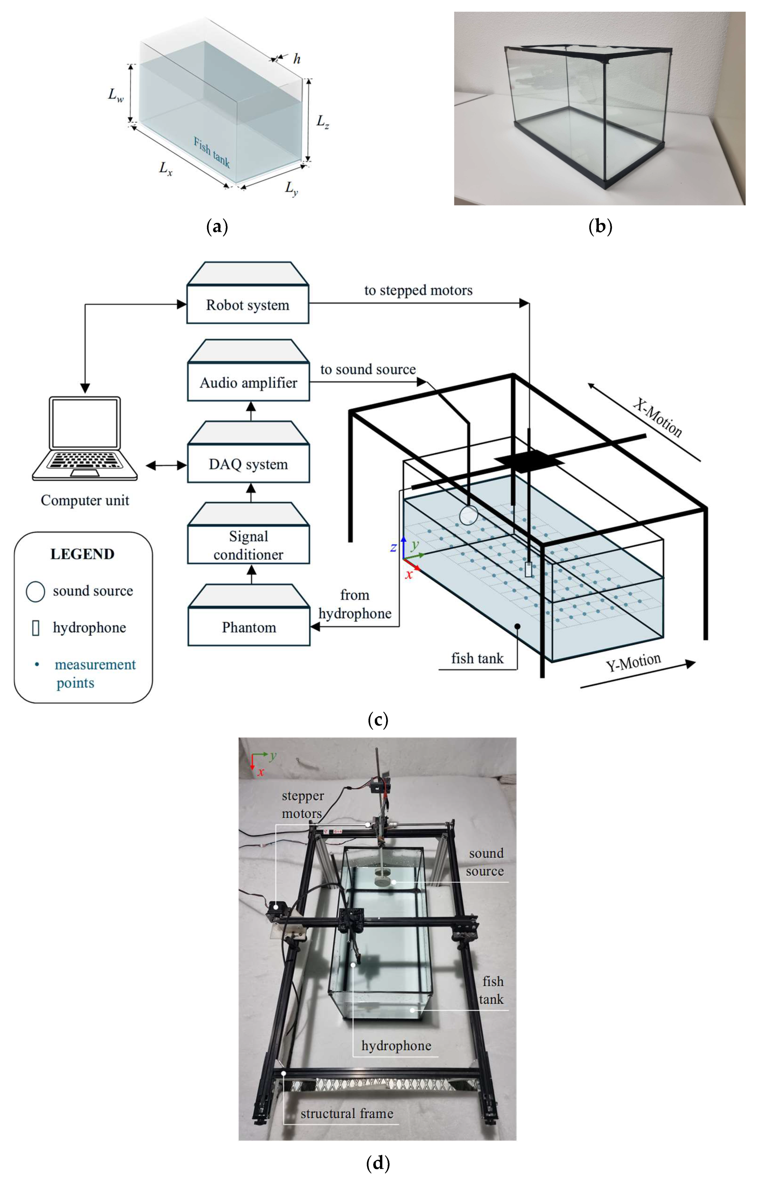
3.1. Fish Tank

Let us consider the schematic representation of a rectangular fish tank shown in Figure 1a. In this scheme, L_x, L_y, and L_z are the dimensions of the tank in a cartesian coordinate system whose origin of coordinates is in one of the bottom corners of the tank, h is the thickness of the walls, and L_w stands for the water filling level. The empty fish tank used for the experiments is depicted in Figure 1b, its dimensions being L_x = 494 mm, L_y = 258 mm, L_z = 293 mm, and h = 3 mm. The tank is made of glass material with an elastic modulus E = 80 GPa and a mass density ρ = 2600 kg/m³, resulting in a c = 5547 m/s, the damping factor η being set to 0.05 using a fitting procedure as in [14]. The properties of the fluids were ρ_a = 1.21 kg/m³ and c_a = 343 m/s for the air over the top surface, and ρ_w = 1000 kg/m³ and c_w = 1500 m/s for the water inside the tank, where ρ_i and c_i stand for the density and speed of sound, respectively. All these parameters are necessary for the prediction model to be described at the end of this section and therefore must be known beforehand.

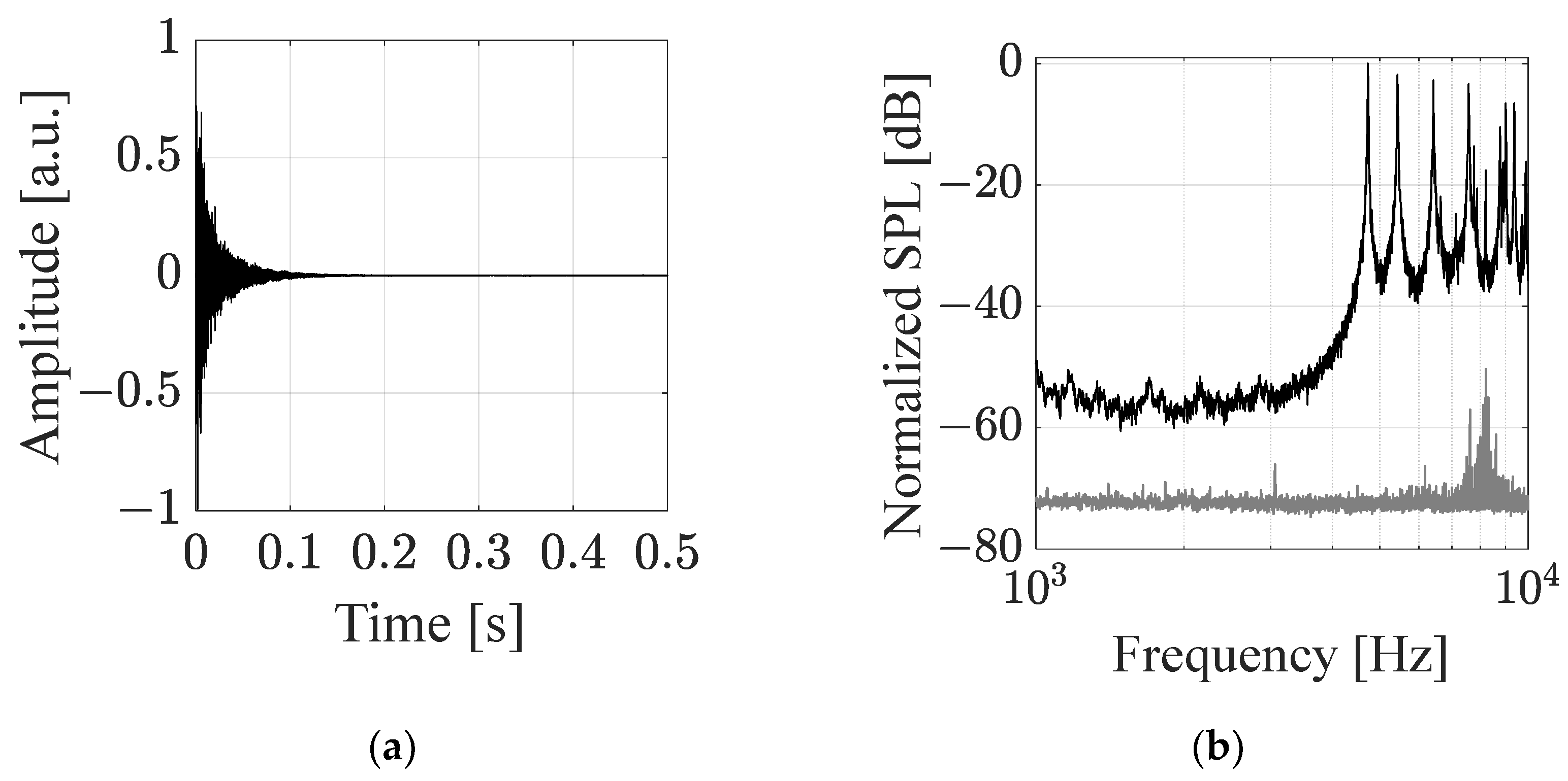
3.2. Measurement System

A scheme of the experimental setup prepared to measure the sound pressure field in the fish tank is shown in Figure 1c. This setup comprised a Cartesian coordinate robot composed of a structural frame with Nema 17 stepper motors (PCB Linear. 6402 E. Rockton Rd. Roscoe, IL 61073. USA) controlled with a microcontroller board Arduino UNO R3 (Arduino S.r.l. Via Andrea Appiani 25, 20900 Monza (MB), Italy. Distribuidor: RS Group plc. Fifth Floor. Two Pancras Square. London. N1C 4AG. UK), two acoustic transducers: a custom-made sound source connected to an audio amplifier PASCO PI-9587C, and an omnidirectional hydrophone AQUARIAN AS-1 (measured sensitivity: −167.5 ± 2 dB re 1 V/μPa, working frequency range from 1 Hz to 10 kHz) connected to a Brüel&Kjaer NEXUS 2692 signal conditioner (Brüel & Kjær Sound & Vibration Measurement A/S DK-2850 Nærum, Denmark; sensitivity 100 mV/Pa, and self-noise lower than 0.01%) via a phantom power supply SHURE PS1A (SHURE Incorporated. 5800 W. Touhy Avenue, Niles, IL 60714-4608, USA max. self-noise in differential mode of 1.78 μV), used to reproduce and record sounds inside the tank, respectively, both connected to a DAQ system NI-USB-6351 (National Instruments Corporate Headquarters—11500 North Mopac Expressway Austin, Texas 78759-3504 USA; random noise of 281 μV in a dynamic range of 10 V) controlled from a computer unit. Different from other works using hydrophone arrays [19,20], the robotic measurement system herein proposed allowed performing measurements in a horizontal plane in the fish tank with a single transducer unit (spatial resolution of 20 mm; total of 252 measurement points per plane was herein used) by using a self-developed Graphical User Interface (GUI) in LabVIEW^® (National Instruments Corporate Headquarters—11500 North Mopac Expressway Austin, Texas 78759-3504 USA). The custom-made sound source herein used consisted of an electrodynamic actuator TECTONIC TEAX19C01-8 (Tectonic Audio Labs. 17802 134th Avenue NE, Suite 17. Woodinville, WA 98072-8806 USA) embedded in a small cylindrical box 60 mm in diameter to achieve a device with a piston-type vibration pattern in the frequency range of analysis (see [21] for details). In this regard, it should be noted that the robotic system does not cover the whole measurement plane due to the space constraints for the sound source and the hydrophone mounting support, resulting in a blind zone within the analyzed area. In general, the directivity of a sound source may influence the sound pressure spatial distribution in a bounded space, such as a fish tank. However, given that the dimensions of the fish tank are close to or below the wavelengths to be analyzed, and the sound field spatial distribution was measured spaced away from the sound source and in steady-state conditions (i.e., the reverberant field dominates over the direct field), the directional features of the sound source may not have a significant influence on the resulting sound field. The type of signal used to feed the sound source was a Maximum-Length Sequence (MLS), whose main advantage is the high Signal-to-Noise (S/N) ratio under unfavorable conditions (i.e., noisy scenarios) [22], also allowing obtaining the impulse time response at any measurement point. The frequency spectra were calculated from the Fast Fourier Transform of these impulse time responses for each recording point using self-developed codes in MATLAB^® software (Mathworks Natick, Apple Hill Campus. 1 Apple Hill Drive. Natick, MA 01760-2098. USA). A detailed view of the measurement setup including the custom-made sound source and the hydrophone mounted in the robotic arm is shown in Figure 1d.

3.3. Novak et al. [14] Model for Water-Filled Rectangular Tanks

Novak et al. used a modal approach to propose an analytical formulation for the acoustic pressure field in a water-filled tank including leakage through the walls [14]. According to their model, the frequency-dependent sound pressure generated in the coordinate (x, y, z) by a point source located in position (x₀, y₀, z₀) can be obtained from

$$p\left(x,y,z\right)={\displaystyle \sum _{m=0}^{\infty }\frac{{\psi }_m\left(x_0,y_0,z_0\right)}{k_m^2-k_w^2}}{\psi }_m\left(x,y,z\right)$$

(1)

where ψ_m is the modal wave function that describes the spatial distribution of the sound field inside the tank for the mth mode and is given by the following equation

$${\psi }_m\left(x,y,z\right)=\sqrt{{\displaystyle \frac{2^3}{L_x{L}_y{L}_z}}}\sin \left(k_{m,x}x-j{\zeta }_x\right)\sin \left(k_{m,y}y-j{\zeta }_y\right)\sin \left(k_{m,z}z-j{\zeta }_z\right)$$

(2)

with

$$k_{m,x}=\left(m_x\pi +j2{\zeta }_x\right)/L_x$$

(3)

$$k_{m,y}=\left(m_y\pi +j2{\zeta }_y\right)/L_y$$

(4)

$$k_{m,z}=\left(m_z\pi +j\left({\zeta }_z+{\zeta }_z^{\prime }\right)\right)/L_z$$

(5)

where m_x, m_y, and m_z are integers that represent the modal indexes for the mth mode in each direction, and ζ_i^(‘) are the modal specific impedances at the boundaries of the fish tank (see Appendix A for details). k_w = ω/c_w is the wave number in water, ω is the angular frequency, and k_m is the modal wave number defined by

$$k_m=\sqrt{k_{m,x}^2+k_{m,y}^2+k_{m,z}^2}$$

(6)

Thereupon, it is straightforward to retrieve the normal frequencies of such a water-filled tank from

$$f_m=k_m{\displaystyle \frac{c_w}{2\pi }}$$

(7)

Note that in the above expression, L_z should equal L_w in the calculation of the normal modes of the water-filled fish tank.

4. Results and Discussion

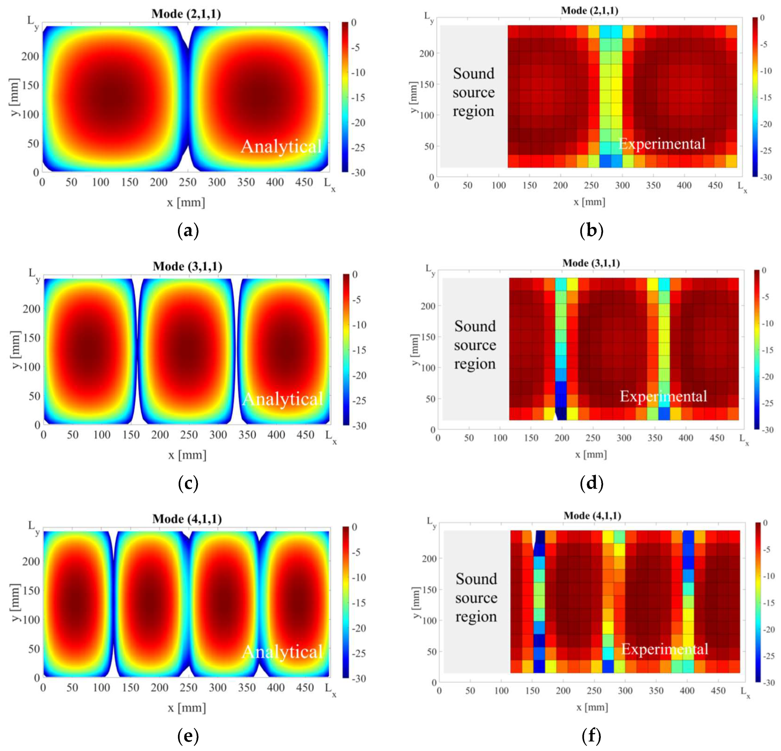
4.1. Normal Modes

First, the experimental setup described in the previous section was used to measure the sound pressure level in a horizontal plane at z = 100 mm in the fish tank when the sound source was positioned in (33, L_y/2, L_w/2) mm and the water level was set to L_w = 200 mm. This choice was considered similar to those configurations typically used in fish tank experiments [14,15,18,19,20] and representative to illustrate the normal modes in the fish tank. Figure 2a shows an example impulse time response at the position (L_x/2, L_y/2, L_w/2) and the normalized sound pressure level (SPL) spectrum averaged in the measurement plane, together with a measurement of the background noise inside the fish tank. Even though all the spectrum results to be discussed hereinafter are normalized to the maximum amplitude value in the frequency range from 1000 Hz to 10 kHz, it is worth pointing out that the dynamic range of the sound pressure field in the fish tank experiments was from 100 μPa (40 dB re 1 μPa) to 0.263 Pa (108.4 dB re 1 μPa), those levels being far above (at least 10 dB) the background noise level (gray line) in the frequency range of analysis.

Next, the theoretical model was used to calculate both the normal modes in the water fluid of the fish tank and to analyze the sound field spatial distribution for some of these modes. The first 10 normal modes obtained from the analytical model and the experimental measurements are listed in

Table 1. Predicted and measured normal frequencies in a fish tank with dimensions 494 mm × 258 mm × 293 mm, and the water level was set to L_w = 200 mm.

Mode *			Normal Frequency (Hz)
mx	my	mz	Analytical	Experimental	Relative Error (%)
1	1	1	4757	4752	0.11
2	1	1	5396	5456	1.10
3	1	1	6319	6449	2.02
1	2	1	6710	6682	0.42
2	2	1	7178	7162	0.22
4	1	1	7421	7628	2.71
3	2	1	7895	7903	0.10
2	1	2	8252	8250	0.02
4	2	1	8802	8855	0.60
1	3	1	9075	9051	0.27

* Mode indexes m_x, m_y, and m_z correspond to the normal frequencies sorted in ascending order.

.

Results indicate good agreement between the normal frequencies calculated using the analytical model and those obtained experimentally, with relative errors below 3%. As expected, the modes of Table 1 are significantly excited or detected in the fish tank measurements as resonance peaks in the frequency spectrum in Figure 2b. To further illustrate it, examples of the sound field spatial distribution obtained using the analytical model and in the experimental measurements are depicted in Figure 3 for three of the modes of vibration excited: mode (2, 1, 1), mode (3, 1, 1), and mode (4, 1, 1). Results show that the analytical model agrees well with the experimental measurements. As described in Section 3.2, the robotic system does not cover the whole measurement plane mainly due to the space requirements of the sound source. Even though some blind spots are caused by the obstruction of both the sound source and the hydrophone, a good agreement can be found between the analytical and experimental results, the accuracy being slightly reduced at the highest modes analyzed due to the spatial resolution used in the experiments (which could also be increased but herein served to illustrate most of the modal shapes).

However, the Novak et al. model does not account for the bending vibration of the fish tank walls (further details on this issue will be given in Section 4.3), and its high-frequency limit of application requires some comments that are worth pointing out. Since the sound pressure field in the fish tank involves more superimposed normal modes as the frequency increases, it will be determined by the number of modal indexes considered for the modal summation in the Novak et al. model. In our work, the maximum values for these indexes were chosen so that convergence was found for the sound pressure spectrum in the frequency range under analysis. Alternatively, Schroeder’s frequency cut-off frequency can be calculated from reverberant behavior, or extra effects such as glass leakage at frequencies above 10 kHz included in the damping factor.

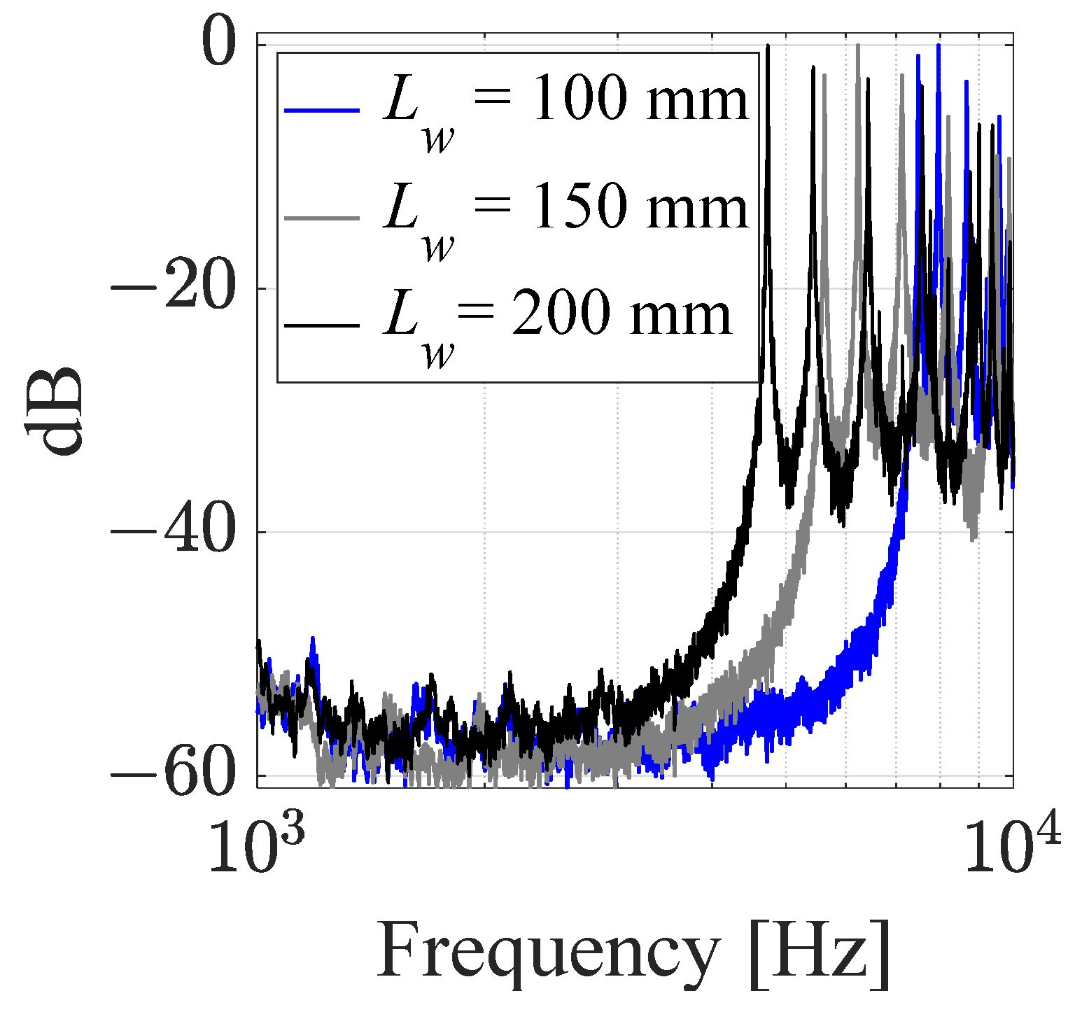
4.2. Parametric Analysis

Once the first normal modes in the fish tank were identified from the sound pressure level measurements and verified using the analytical model, it was found useful to perform a parametric analysis to study the effect on the experiments of parameters such as the water level, the measurement depth, and the sound source power.

4.2.1. Water Level

First, a discussion on the influence of using different water levels on the normal modes in the fish tank was carried out. As pointed out by Akamatsu et al. [18], the first resonant frequency in a small tank is expected to increase as the water level of the tank is reduced. In our experiments, the water level L_w was set to 100 mm, 150 mm, and 200 mm; all the measurements were performed in the mid-height plane for each water level. The sound source is thus positioned in (33, L_y/2, L_w/2) mm. Figure 4 shows the sound pressure level spectrum averaged over the measurement plane for each water level.

The above results show that not only the first resonant frequency but also the higher-order modes shift towards higher frequencies as the water level is reduced, thus modifying the sound field spatial distribution in each case and therefore are expected to influence the assessment of noise effects in fish. It should be noted that not all the modes are shifted equally, as this shift will depend on the width-depth ratios and therefore on the dimensions of the fish tank under analysis. In this regard, the availability of a predictive tool like that used in the current work may help outline the experimental setup. Hereinafter, only the fish tank configuration with L_w = 200 mm will be analyzed.

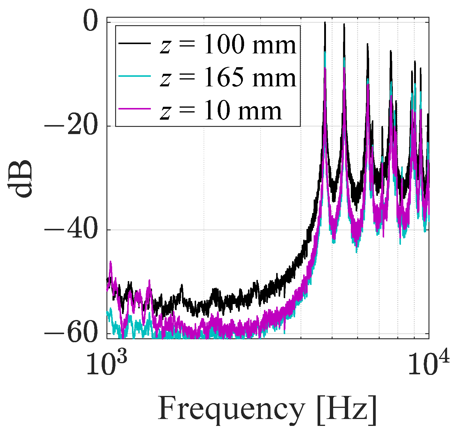
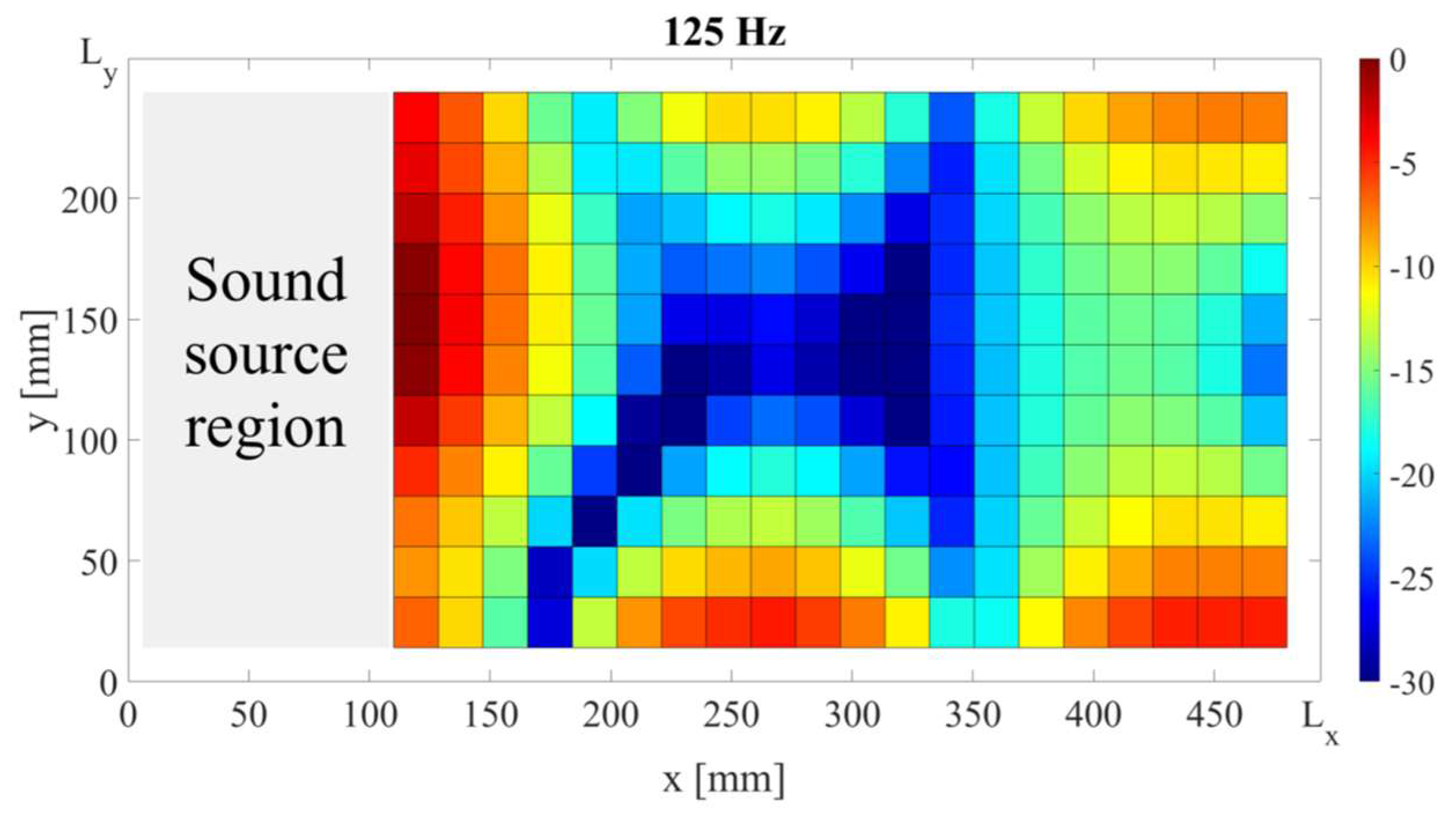
4.2.2. Measurement Depth

Next, the influence of measuring the sound pressure level at different depths in the fish tank was analyzed. To this end, the sound pressure was measured at different planes: z = 10 mm, z = 100 mm, and z = 165 mm; and the resulting average sound pressure level was examined. Figure 5 shows the corresponding frequency spectra.

Results indicate that those measured planes at depths close to boundary surfaces, either the top surface (air) or bottom surface (glass), show lower sound pressure levels than the mid-plane at which the sound source is located. Consequently, the lower levels near these surfaces may explain fish swimming upwards or downwards in those experiments in which a noise source is placed inside the fish tank [2,20,23]. Nevertheless, this is a remark that still needs further investigation and that would require a more detailed analysis involving fish inside the tank.

4.2.3. Sound Source Power

An important source of uncertainty in bioacoustics experiments is commonly linked to the type of transducer used as a sound source. In this regard, significant differences can be found in the frequency response given that its performance depends not only on the electrical power supplied to the source but also on its electrical and mechanical parameters [24]. In Figure 6, the sound pressure level averaged over a measurement plane at z = 100 mm is shown for different power gains, G: 2, 1.5, and 1 (reference).

In the previous plot, the sound level increase from the reference gain (G = 1) was around 3.5 dB for G = 1.5 and around 6 dB for G = 2 at frequencies below the first normal mode. Despite the measurements being performed in a reverberant space whose sound field is dependent on the properties of the fish tank (i.e., dimensions, wall material, losses…), this data was similar to that expected if measurements were carried out in free-field conditions. Zhang et al. [25] already showed that a sound field transfer relationship can be obtained from the reverberant field of a water-filled tank to the free field below the so-called Schroeder cut-off frequency. However, this linear relation is no longer fulfilled if the sound field distribution is not homogeneous, as in higher-order modes, where increments between power gains are less than 1 dB.

4.3. Remarks on the Low-Frequency Behavior of Fish Tanks

In practice, not only do the normal modes in the fish tank need to be considered but the bending motion due to the vibration of the walls also needs to be considered, especially in the low-frequency range. Even though the full acoustic-structural modeling of the fish tank may turn its analysis quite complex [26] and is beyond the scope of the current work, the authors found it of interest to illustrate this low-frequency modal behavior. To do so, the spatial sound level distribution was analyzed at 125 Hz (a typical low frequency in many underwater noise studies) for the reference configuration whose results were presented in Section 4.1. Figure 7 shows the resulting sound level field.

Unlike the sound field spatial distributions shown for normal modes in Figure 3, the above plot suggests that maximum levels occur in the form of lobes not only close to the sound source but also to the walls of the fish tank. These lobes may be attributed to evanescent bending fields, which usually predominate near boundaries in sound enclosures [27]. Considering these effects in the theoretical model would require, on the one hand, a knowledge of the distribution of vibration modes over the fish tank walls so that, if the modal density is high enough, the system can be analyzed using alternative approaches such as the Statistical Energy Analysis (SEA) method. In this regard, it should be noted that the coupling between structural bending modes and normal modes in the fluid may play an important role, especially in a discrete frequency analysis. Given that in our study, the bending vibrations have a much lower contribution in terms of total acoustic energy in the water when compared to the normal modes (see Figure 2 and Figure 4, Figure 5 and Figure 6), these effects were neglected in the theoretical model (further research on this issue is currently being carried out by the authors). Alternatively, more complex models relying on numerical schemes such as the Finite Element Method (FEM) and the Boundary Element Method (BEM) may be more appropriate.

To further illustrate the importance of the sound field spatial distribution when using fish tank setups for bioacoustics research, the sound pressure level spectrum obtained at all 252 measurement points for the reference configuration analyzed in Section 4.1 is presented in Figure 8.

The above plot further confirms that assuming a homogeneous sound field distribution in the fish tank or just considering the sound level at a single measurement point may lead to wrong conclusions in the analysis of fish behavior under noise conditions. Acoustic experiments in fish tanks are subjected to great uncertainty due to the reverberant sound field, especially in the low-frequency range with differences between points of up to 40 dB (see Figure 8), an issue that is worth further analyzing in the future. Even though some recent studies have proposed the use of expanded polystyrene [28] or submerging the tank in water [29] to dampen reverberation and resonances resulting from sound reflections, there is still a need for new materials that can dampen sound waves in the low-frequency range where fish hearing sensitivity is higher [2]. It is noteworthy that the influence of the noise produced by water pumps, oxygenation, and filtering systems on the low-frequency background noise is also an issue that needs further attention, especially in land-based water tank facilities [30]. Hence, the application of innovative solutions such as underwater acoustic metamaterials [31] in fish tanks will presumably be an interesting research area to explore in the forthcoming years.

5. Conclusions

In this work, an in-depth acoustic analysis of fish tanks commonly used for bioacoustics research was performed. To this end, predictions using a theoretical approach and experimental measurements using a robotized system were carried out to study the sound field spatial distribution in a fish tank in the frequency range in which normal modes exist. The prediction model implemented, which accounted for the damping of the fish tank walls, showed good agreement when compared to the experiments in terms of frequency modes and sound field distribution. On the other hand, preliminary results show that this distribution depends on the frequency of the generated sound and highlights the importance of factors such as the water level, the measurement depth, and the sound source power for developing acoustic experiments in fish tanks. In brief, results show that a decrease in the water level shifts the resonant modes to higher frequencies. As for the measurement depth, those planes near the top and bottom surfaces yield lower sound levels, whereas an increase in the sound source power shows a non-linear increase in the levels at these modes. In addition, an overview of the frequency spectrum at all measurement points in one of these planes illustrates the significant level differences among them, thus confirming the importance of the sound field spatial distribution.

In general, the above results not only showed the potential of using a prediction model to study the acoustic response of fish tanks but also highlighted the importance of analyzing the sound field spatial distribution before preparing these setups to better understand the behavior of fish. Moreover, different from stationary (e.g., tonal, wideband noises…) and transient (e.g., ship noise) signals commonly used in fish tank experiments, the MLS signal proposed allows obtaining the impulse response at any measurement point, which may be very useful for the analysis of transient phenomena such as sound reflections (especially for those sounds whose wavelength is small compared to the fish tank size). This latter feature may be of great help in the design stage of passive solutions to reduce the anthropogenic noise or even control the sound field not only in fish tanks [32] but also in offshore tanks [33]. In summary, the authors hope the results of this work contribute towards the development of methodologies to be used not only in the design stage of fish tanks but also extended to water tanks with larger dimensions, showing their potential capabilities for underwater acoustics research applications.

References

1. Popper, A.; Hastings, M. The effects of anthropogenic sources of sound on fishes. J. Fish Biol. 2009, 75, 455–489. [Google Scholar] [CrossRef] [PubMed]
2. Popper, A.N.; Hawkins, A.D. An overview of fish bioacoustics and the impacts of anthropogenic sounds on fishes. J. Fish Biol. 2019, 94, 692–713. [Google Scholar] [CrossRef]
3. Hildebrand, J.A. Anthropogenic and natural sources of ambient noise in the ocean. Mar. Ecol. Prog. Ser. 2009, 395, 5–20. [Google Scholar] [CrossRef]
4. Weilgart, L. The impacts of anthropogenic ocean noise on cetaceans and implications for management. Can. J. Zool. 2007, 85, 1091–1116. [Google Scholar] [CrossRef]
5. Jézéquel, Y.; Julien, B.; Coston-Guarini, J.; Chauvaud, L. Revisiting the bioacoustics of European spiny lobsters Palinurus elephas: Comparison of antennal rasps in tanks and in situ. Mar. Ecol. Prog. Ser. 2019, 615, 143–157. [Google Scholar] [CrossRef]
6. Hang, S.; Zhao, J.; Ji, B.; Li, H.; Zhang, Y.; Peng, Z.; Zhou, F.; Ding, X.; Ye, Z. Impact of underwater noise on the growth, physiology and behavior of Micropterus salmoides in industrial recirculating aquaculture systems. Environ. Pollut. 2021, 291, 118152. [Google Scholar] [CrossRef] [PubMed]
7. Anderson, P.A. Acoustic characterization of seahorse tank environments in public aquaria: A citizen science project. Aquacult. Eng. 2013, 54, 72–77. [Google Scholar] [CrossRef]
8. Au, W.W.L.; Hastings, M.C. Principles of Marine Bioacoustics; Springer: New York, NY, USA, 2008. [Google Scholar]
9. Parvulescu, A. The acoustics of small tanks. Mar. Bioacoustics 1967, 2, 7–13. [Google Scholar]
10. Lucke, K.; MacGillivray, O.; Halvorsen, M.B.; Ainslie, M.A.; Zeddies, D.G.; Sisneros, J.A. Recommendations on bioacoustical metrics relevant for regulating exposure to anthropogenic underwater sound. J. Acoust. Soc. Am. 2024, 156, 2508–2526. [Google Scholar] [CrossRef]
11. Rogers, P.H.; Hawkins, A.D.; Popper, A.N.; Fay, R.R.; Gray, M.D. Parvulescu revisited: Small tank acoustics for bioacousticians. In The Effects of Noise on Aquatic Life II; Popper, A.N., Hawkins, A.D., Eds.; Springer: New York, NY, USA, 2016; pp. 933–941. [Google Scholar]
12. Li, Q.; Xing, J.; Tang, R.; Zhang, Y. Finite-element method for calculating the sound field in a tank with impedance boundaries. Math. Probl. Eng. 2020, 2020, 6794760. [Google Scholar] [CrossRef]
13. Duncan, A.J.; Lucke, K.; Erbe, C.; McCauley, R.D. Issues associated with sound exposure experiments in tanks. Proc. Mtgs. Acoust. 2016, 27, 070008. [Google Scholar] [CrossRef]
14. Novak, A.; Bruneau, M.; Lotton, P. Small-sized rectangular liquid-filled acoustical tank excitation: A modal approach including leakage through the walls. Acta Acust. United Acust. 2018, 104, 586–596. [Google Scholar] [CrossRef]
15. Campbell, J.; Shafiei Sabet, S.; Slabbekoorn, H. Particle motion and sound pressure in fish tanks: A behavioral exploration of acoustic sensitivity in the zebrafish. Behav. Process. 2019, 164, 38–47. [Google Scholar] [CrossRef] [PubMed]
16. Filiciotto, F.; Vazzana, M.; Celi, M.; Maccarrone, V.; Ceraulo, M.; Buffa, G.; Di Stefano, V.; Mazzola, S.; Buscaino, G. Behavioral and biochemical stress responses of Palinurus elephas after exposure to boat noise pollution in tank. Mar. Pollut. Bull. 2014, 84, 104–114. [Google Scholar] [CrossRef]
17. Fu, Y.; Kabir, I.; Yeoh, G.H.; Peng, Z. A review on polymer-based materials for underwater sound absorption. Polym. Test. 2021, 96, 107115. [Google Scholar] [CrossRef]
18. Akamatsu, T.; Okumura, T.; Novarini, N.; Yan, H.Y. Empirical refinements applicable to the recording of fish sounds. J. Acoust. Soc. Am. 2002, 112, 3073–3082. [Google Scholar] [CrossRef]
19. Tang, R.; Zhang, Y.; Li, Q.; Shang, D. The investigation of the methods for predicting the sound field in a non-anechoic tank with elastic boundary. In Proceedings of the 2016 IEEE/OES China Ocean Acoustics (COA), Harbin, China, 9–11 January 2016. [Google Scholar]
20. Pieniazek, R.H.; Mickle, F.; Higgs, D.M. Comparative analysis of noise effects on wild and captive freshwater fish behavior. Anim. Behav. 2020, 168, 129–135. [Google Scholar] [CrossRef]
21. Poveda-Martínez, P.; Carbajo-San-Martín, J.; Martínez-Iranzo, J.; Segovia-Eulogio, G.; Tinivella, U.; Cianferra, M.; Ramis-Soriano, J. Primeros pasos en el diseño de sistema radiante del tipo DML para acústica submarina. In Tecniacústica 2023; Sociedad Española de Acústica (SEA): Cuenca, Spain, 2023. (In Spanish) [Google Scholar]
22. Vorländer, M.; Kob, M. Practical aspects of MLS measurements in building. Appl. Acoust. 1997, 52, 239–258. [Google Scholar] [CrossRef]
23. Andersson, M.; Svensson, O.; Swartz, T.; Manera, J.L.; Bertram, M.G.; Blom, E.L. Increased noise levels cause behavioral and distributional changes in Atlantic cod and saithe in a large public aquarium—A case study. Aquacult. Fish Fish. 2023, 3, 447–458. [Google Scholar] [CrossRef]
24. Beranek, L.; Mellow, T. Acoustics: Sound Fields and Transducers; Academic Press: Oxford, UK, 2012. [Google Scholar]
25. Zhang, Y.M.; Tang, R.; Li, Q.; Shang, D.J. The investigation of the method for measuring the low-frequency radiated sound power in a reverberation tank. Proc. Mtgs. Acoust. 2016, 29, 070002. [Google Scholar] [CrossRef]
26. Rezaiee-Pajand, M.; Aftabi S, A.; Kazemiyan, M. Analytical solution for free vibration of flexible 2D rectangular tanks. Ocean Eng. 2016, 122, 118–135. [Google Scholar] [CrossRef]
27. Fahy, F.; Gardonio, P. Sound and Structural Vibration: Radiation, Transmission and Response, 2nd ed.; Academic Press: Oxford, UK, 2007. [Google Scholar]
28. Olivier, F.; Gigot, M.; Mathias, D.; Jezequel, Y.; Meziane, T.; L’Her, C.; Chauvaud, L.; Bonnel, J. Assessing the impacts of anthropogenic sounds on early stages of benthic invertebrates: The “Larvosonic system. ” Limnol. Oceanogr. Meth. 2022, 21, 53–68. [Google Scholar] [CrossRef]
29. Holgate, A.; White, P.R.; Leighton, T.; Kemp, P.S. Sound fields in two small experimental test arenas: A comparison. In The Effects of Noise on Aquatic Life: Principles and Practical Considerations; Popper, A.N., Sisneros, J.A., Hawkins, A.D., Thomsen, F., Eds.; Springer: Cham, Switzerland, 2024; pp. 61–74. [Google Scholar]
30. Ramis, J.; Poveda, P.; Carbajo, J.; Ullah, N.; Ramis, E.; Forcada, A.; Valle, C.; Espinosa, V.; Pérez-Arjona, I.; Ortega, A.; et al. Estudio del efecto del ruido antropogénico en atunes en cautividad. In FIA 2024; Sociedad Chilena de Acústica (SOCHA): Santiago de Chile, Chile, 2024. (In Spanish) [Google Scholar]
31. Dong, E.; Cao, P.; Zhang, J.; Zhang, S.; Fang, N.X.; Zhang, Y. Underwater acoustic metamaterials. Natl. Sci. Rev. 2023, 10, nwac246. [Google Scholar] [CrossRef] [PubMed]
32. Wiegerink, J.; Baldock, T.; Callaghan, D.; Wang, C. Experimental study on hydrodynamic response of a floating rigid fish tank model with slosh suppression blocks. Ocean Eng. 2023, 273, 113772. [Google Scholar] [CrossRef]
33. Chu, Y.; Wang, C.; Park, J.; Lader, P. Review of cage and containment tank designs for offshore fish farming. Aquaculture 2020, 519, 734928. [Google Scholar] [CrossRef]
Figure 1. Materials and methods used in the current research: (a) Schematic representation of a fish tank, (b) Picture of the empty fish tank used for the experiments, (c) scheme of the experimental setup used to perform the sound pressure measurements in the fish tank, and (d) detailed view of the experimental setup.
Jmse 13 01253 g001
Figure 2. (a) Impulse time response at the position (Lx/2, Ly/2, Lw/2), and (b) normalized sound pressure level (SPL) spectrum averaged in a horizontal plane at z = 100 mm in a fish tank with dimensions 494 mm × 258 mm × 293 mm when a sound source was positioned in (33, Ly/2, Lw/2) mm and the water level was set to Lw = 200 mm, together with the background noise level (gray line).
Jmse 13 01253 g002
Figure 3. Sound field spatial distribution in the fish tank under analysis at normal frequencies. (a) Mode (2, 1, 1) (analytical), (b) mode (2, 1, 1) (experimental), (c) mode (3, 1, 1) (analytical), (d) mode (3, 1, 1) (experimental), (e) mode (4, 1, 1) (analytical), and (f) mode (4, 1, 1) (experimental).
Jmse 13 01253 g003
Figure 4. Sound pressure level spectrum averaged in a horizontal plane for different water levels Lw: 100 mm (blue line), 150 mm (gray line), and 200 mm (black line, reference).
Jmse 13 01253 g004
Figure 5. Sound pressure level spectrum averaged in horizontal planes at different heights z: 100 mm (black line, reference), 165 mm (cyan line), and 10 mm (magenta line).
Jmse 13 01253 g005
Figure 6. Sound pressure level spectrum averaged in horizontal planes at z = 100 mm for different sound source power gains G: 2 (red line), 1.5 (yellow line), and 1 (green line, reference).
Jmse 13 01253 g006
Figure 7. Sound field spatial distribution in the fish tank under analysis at 125 Hz.
Jmse 13 01253 g007
Figure 8. Sound pressure level spectra at all measurement points (gray lines) and the average (black line) for the reference configuration analyzed in Section 4.1.
Jmse 13 01253 g008