Hydrodynamic and Vibroacoustic Simulation Analysis of the Main Float in an Acoustic Submerged Buoy System

Abstract

During prolonged deployment, deep-sea acoustic submerged buoys may undergo displacement and torsional deformation of their main floating body under turbulent flows, which degrades the quality of acquired sensor data and introduces vibration-induced noise that interferes with acoustic measurements. This paper presents a novel structural design for acoustic buoy main bodies based on hydrodynamic principles. We performed fluid-structure interaction (FSI) simulations to evaluate the dynamic response characteristics of the structure in deep-sea conditions, including computational analysis of velocity and pressure field distributions surrounding the buoy. Leveraging pressure data derived from computational fluid dynamics (CFD) simulations, we developed an innovative vibration noise quantification methodology. This approach employs plane wave excitation with equivalent pressure magnitude to simulate hydrodynamic loading effects while incorporating tripartite coupling mechanisms among fluid, structural, and acoustic domains. The simulated vibration noise profiles establish environmental baseline noise levels for onboard acoustic monitoring instruments, thereby enhancing measurement fidelity.

1. Introduction

In recent years, with the increasing strategic significance of the ocean, China has placed greater emphasis on marine affairs and has gradually formulated and refined its strategic plans for marine development. Driven by advancements in marine scientific research, the comprehensive development and utilization of marine resources, and national defense initiatives, China’s investment in marine environmental monitoring has continued to grow, leading to a significant rise in the demand for underwater environmental monitoring instruments and equipment [1]. Against this backdrop, the marine submerged buoy system, as a crucial monitoring tool, has been increasingly utilized in China. This system is primarily employed for the long-term and stable monitoring of key marine environmental parameters, such as water temperature, salinity, current velocity, and underwater noise, providing essential data support for marine scientific research, resource development, and national defense security [2,3].

Since the dawn of the 21st century, China has formally initiated a strategy to transform itself into a maritime powerhouse, implemented comprehensive and systematic planning for national marine development, and emphasized the strategic importance of innovation and advancement in marine science and technology. With the rapid development of the marine economy, challenges related to marine energy, seabed resources, and maritime security have become increasingly prominent, making real-time and reliable monitoring systems essential for ensuring maritime security [4]. In the field of marine monitoring, the submerged buoy system, as a crucial technological tool, has been widely applied in underwater target detection, acoustic monitoring, and early warning for maritime security [5]. By utilizing the submerged buoy system, long-term, continuous, and covert monitoring in the marine environment can be achieved. This system not only effectively detects moving targets underwater but also collects a wide range of marine environmental data.

However, traditional submerged buoy monitoring systems can only retrieve monitoring data after the system has been recovered, making it inefficient for obtaining real-time observational data. Moreover, during long-term operation, submerged buoys may experience significant drift and subsidence due to unexpected conditions. In extreme cases, unexpected events during retrieval may even lead to recovery failure, resulting in the loss of critical data and economic losses. Since acoustic submerged buoys are equipped with hydrophones, the influence of background noise from ocean currents and flow-induced noise on the hydrophone must also be considered [6]. Therefore, developing an acoustic submerged buoy system that is covert, stable, capable of long-term operation, and capable of providing real-time monitoring data, along with conducting hydrodynamic and acoustic simulations, is of great scientific and practical significance.

Internationally, in 2020, the Woods Hole Oceanographic Institution in the United States employed LES simulations to analyze the wake field of moored buoys, proposing an adaptive tail design to suppress vortex shedding [7]. The French IFREMER Research Institute developed the “MOOSE” moored buoy network, equipped with wideband hydrophones. In 2022, they proposed a multi-dimensional coupled simulation method combining CFD and DEM (Discrete Element Method) to simulate the impact of biological fouling on mooring flow fields [8]. As researchers set new requirements for simulation accuracy and computing power. In China, Song Baowei [9] utilized LES methods and Lighthill acoustic analogy theory to study the flow-induced noise characteristics of underwater vehicles. Many scholars have also employed the Reynolds-averaged Navier-Stokes equation (RANS) turbulence model to calculate flow fields and the FW-H equation to calculate pressure pulsation noise [10]. Based on existing research results, noise calculation methods based on acoustic analogy theory exhibit reasonable agreement between predicted results and experimental data [11].

Based on the current challenges in the research and development of acoustic submerged buoys, this paper proposes a real-time transmission acoustic submerged buoy system utilizing an underwater winch, primarily designed for monitoring and real-time transmission of acoustic signals in deep and remote ocean environments. This type of acoustic submerged buoy enables the deployment and retrieval of a communication float via the underwater winch, and, when integrated with the Beidou Navigation Satellite System, facilitates real-time data transmission [12,13,14]. To ensure the stable posture of the buoy and minimize environmental noise interference on the hydrophone, critical observation instruments, such as hydrophones, are mounted on the main floating body of the buoy.

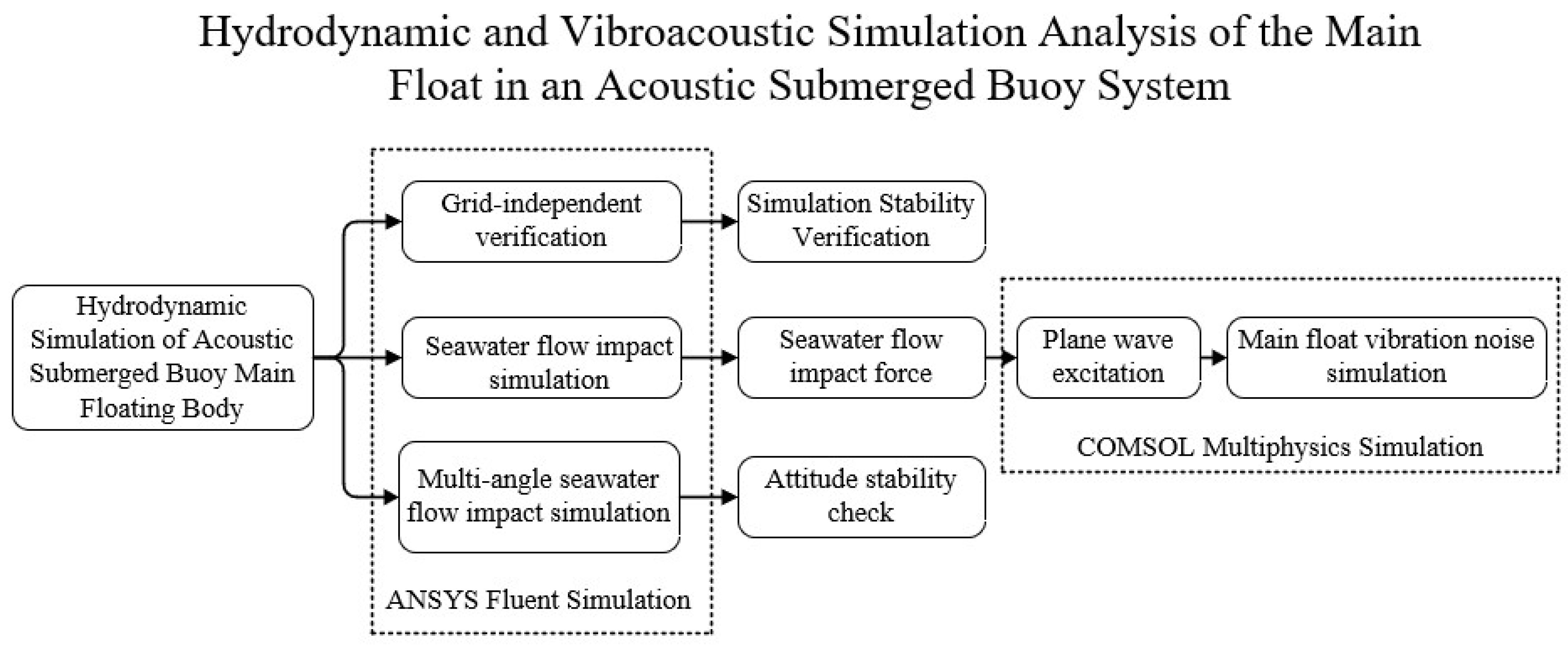
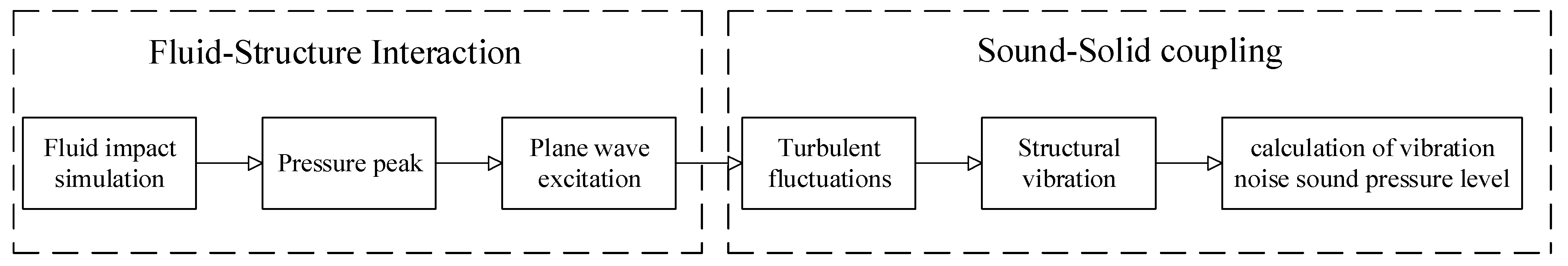
In this study, ANSYS Fluent 2022 R1 and COMSOL Multiphysics 6.1 are employed to analyze the hydrodynamic performance and noise characteristics of the acoustic submerged buoy. This paper utilizes pressure data obtained from computational fluid dynamics (CFD) simulations to develop an innovative method for quantifying vibration noise. This method employs plane wave excitation with equivalent pressure magnitude to simulate the effects of fluid dynamic loads while integrating a three-way coupling mechanism between the fluid, structural, and acoustic domains. Fluid-structure coupling calculations are performed in Fluent, and the pressure peak results from the Fluent calculations are then input into COMSOL for acoustic-structure coupling calculations. This article evaluates the impact of pressure and relative velocity of the main buoy of an underwater buoy under a flow velocity of 0.3 m/s. Its structure has been optimized to achieve better stability. Using a new flow noise calculation method, it was found that under a flow velocity of 0.3 m/s, the vibration noise calculation result at the front end of the main buoy is approximately 47.856 dB. The flowchart of the paper is presented as follows (Figure 1).

The main research content is as follows:

• Based on the real-time transmission acoustic submerged buoy system, a primary buoy suitable for this system was specifically designed. Instrumentation was integrated and mounted, forming a cohesive structure for the entire submerged buoy system.
• Given the unknown deep-sea environment in which the submerged buoy operates, the main buoy body may experience rotational motion due to turbulence. Ansys Fluent was employed to simulate current-induced impacts, evaluate the motion behavior and dynamic response of the submerged buoy system under known ocean current conditions, and further propose optimization strategies to improve the overall system structure.
• To meet the requirements of acoustic submerged buoys, a novel approach for calculating acoustic flow noise was proposed using COMSOL Multiphysics. By referencing the results of dynamic simulations, pressure waves of equivalent magnitude were employed to simulate the impact of ocean currents. The study analyzes the vibration noise generated by ocean currents striking the buoy and its effect on the hydrophones mounted on the acoustic submerged buoy. The goal is to minimize noise interference with hydrophone monitoring and enhance monitoring accuracy.

2. Structure and Modeling of Submerged Buoy System

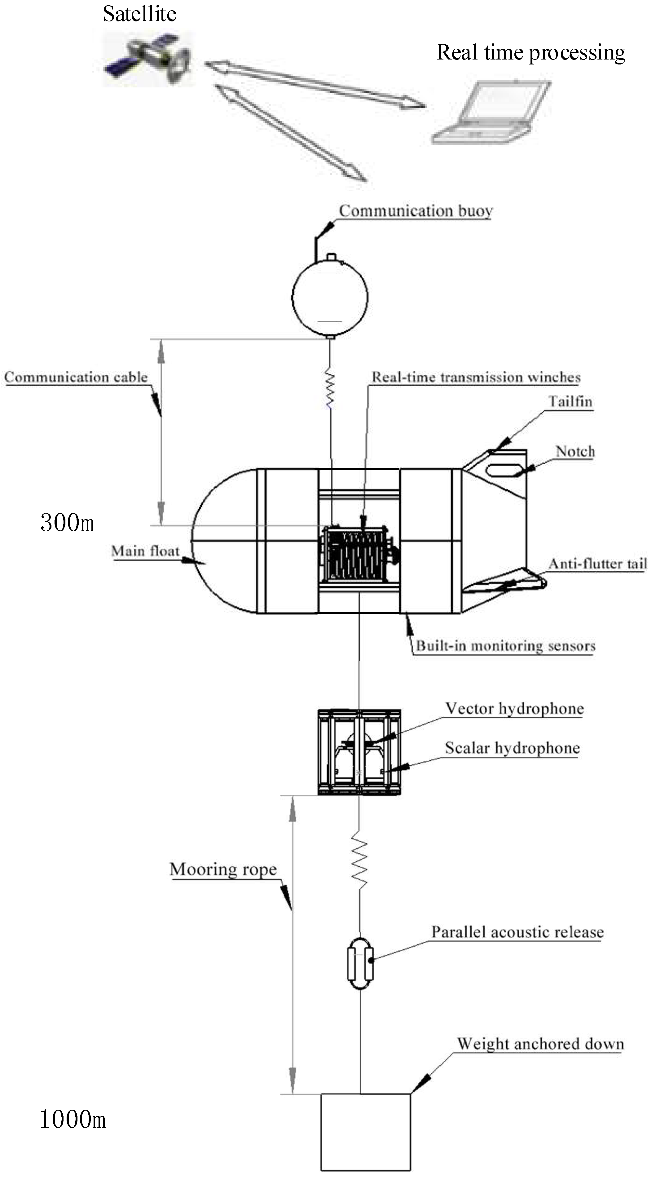
The acoustic submerged buoy system investigated in this paper comprises a main float (buoy body), a communication buoy, an acoustic hydrophone, an underwater winch, detection instruments, floatation spheres, a mooring system, and an acoustic release mechanism. Specifically, the main float is deployed at a depth of 300 m below the sea surface to mitigate surface disturbances. The communication buoy is suspended in the upper water column above the main float, adjusting its depth according to communication requirements. The acoustic hydrophone is housed within a serrated protective frame positioned at a designated location beneath the main float. The underwater winch, mounted on the main float, coordinates with the communication buoy’s depth adjustments. Detection instruments are uniformly distributed along the mooring cable of the submerged buoy. The mooring system secures the entire assembly to a predetermined point on the seabed. Along the mooring line between the main float and the anchor, multiple floatation spheres are attached at various depths as needed. An acoustic release mechanism is installed at the junction of the mooring line and the anchor [15]. The system components are illustrated below (Figure 2).

The main float serves as the core component of the submerged buoy system. Its performance directly determines whether the system can operate stably over extended periods in unknown marine environments, while its structural design is critical for ensuring stability and attitude control [16]. The design of the main float structure should take into account the low center of gravity of the main float; the lower the center of gravity is below the center of buoyancy, the better. The submerged buoy system studied in this paper is deployed at a site in the South China Sea, with the main float located at 300 m below the water surface, where the water temperature is 10–12 °C and the salinity is 34.4–34.6 PSU. $Re\approx 2.77\times {10}^5$, which belongs to the turbulent flow condition with high Reynolds number. Considering practical research and development requirements, the main float should adopt a horizontal configuration with excellent current resistance. It must maintain normal functionality under surface currents of up to 3 knots (1.54 m/s). At a depth of 300 m, where current speeds typically range between 5% and 20% of surface velocities (approximately 0.08 to 0.31 m/s), this study focuses on extreme flow conditions to investigate the behavioral characteristics and dynamic response of the main float under a current of 0.3 m/s.

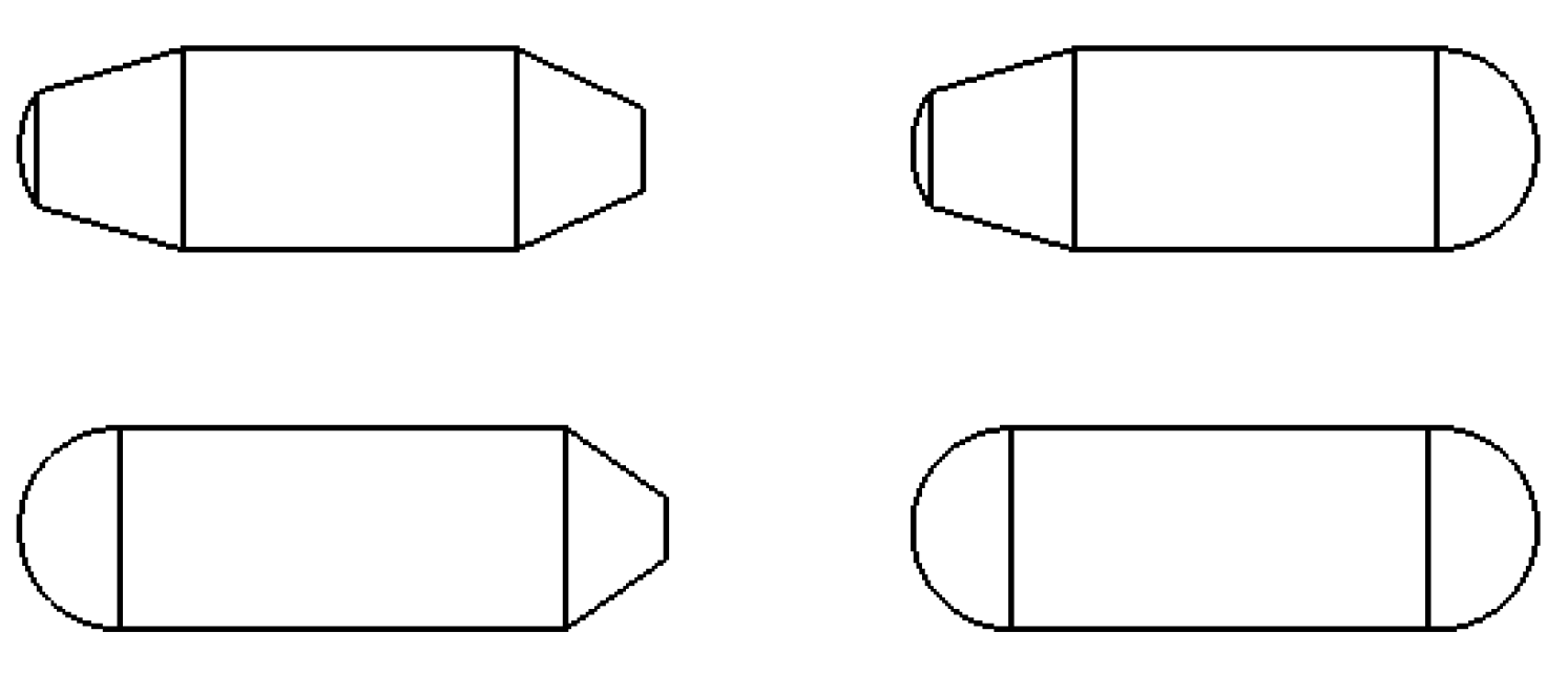
The first step involves determining the structure of the main float. In this paper, several models were constructed sequentially for simulation and optimization. Although the structure of each model is different, the diameter and length of the models are the same (2.45 m in length and 0.9 m in diameter) in consideration of controlling the simulation variables. Drawing on the design principles of underwater vehicles, the main float structure can be categorized into four types based on the transition features at the head and tail: streamlined and semi-circular configurations. A streamlined transition reduces hydrodynamic resistance but increases the overall length of the float. Conversely, a semi-circular transition decreases the characteristic length of the float but increases its resistance. As illustrated in the figure below (Figure 3), Model I, which employs streamlined transitions at both the head and tail, exhibits the lowest resistance but requires the largest characteristic length, potentially resulting in an excessively large main float Model II, featuring a streamlined transition at the head and a semi-circular transition at the tail, may lead to uneven buoyancy distribution, with the head experiencing significant flow-induced offset rotation. Model IV, utilizing semi-circular transitions at both ends, achieves the smallest characteristic length but incurs excessive flow resistance. Model III, however, demonstrates relatively low resistance and an optimal characteristic length. A preliminary fluid simulation was conducted to evaluate the four structural types, and the most suitable design was selected as the basis for the main float development.

A numerical simulation approach based on hydrodynamic principles was employed, utilizing ANSYS Fluent for preliminary simulations. Three-dimensional models of the four proposed float structures (Model I, II, III, and IV) were constructed and subjected to initial current impact simulations. The velocity and pressure distributions resulting from the impact were analyzed, and the most suitable float structure was selected for further design optimization. The three-dimensional models of the four structures are shown in Figure 4.

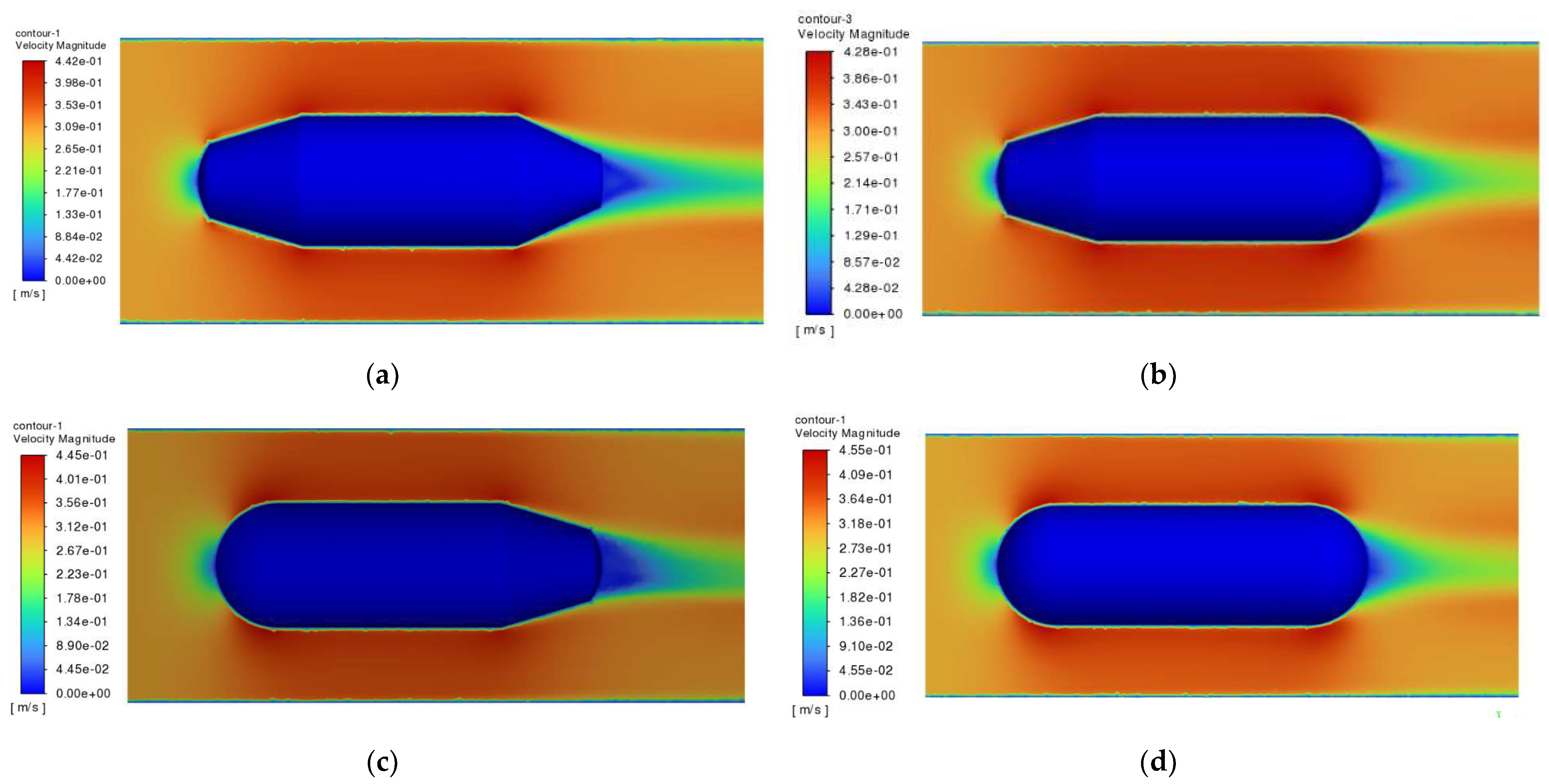
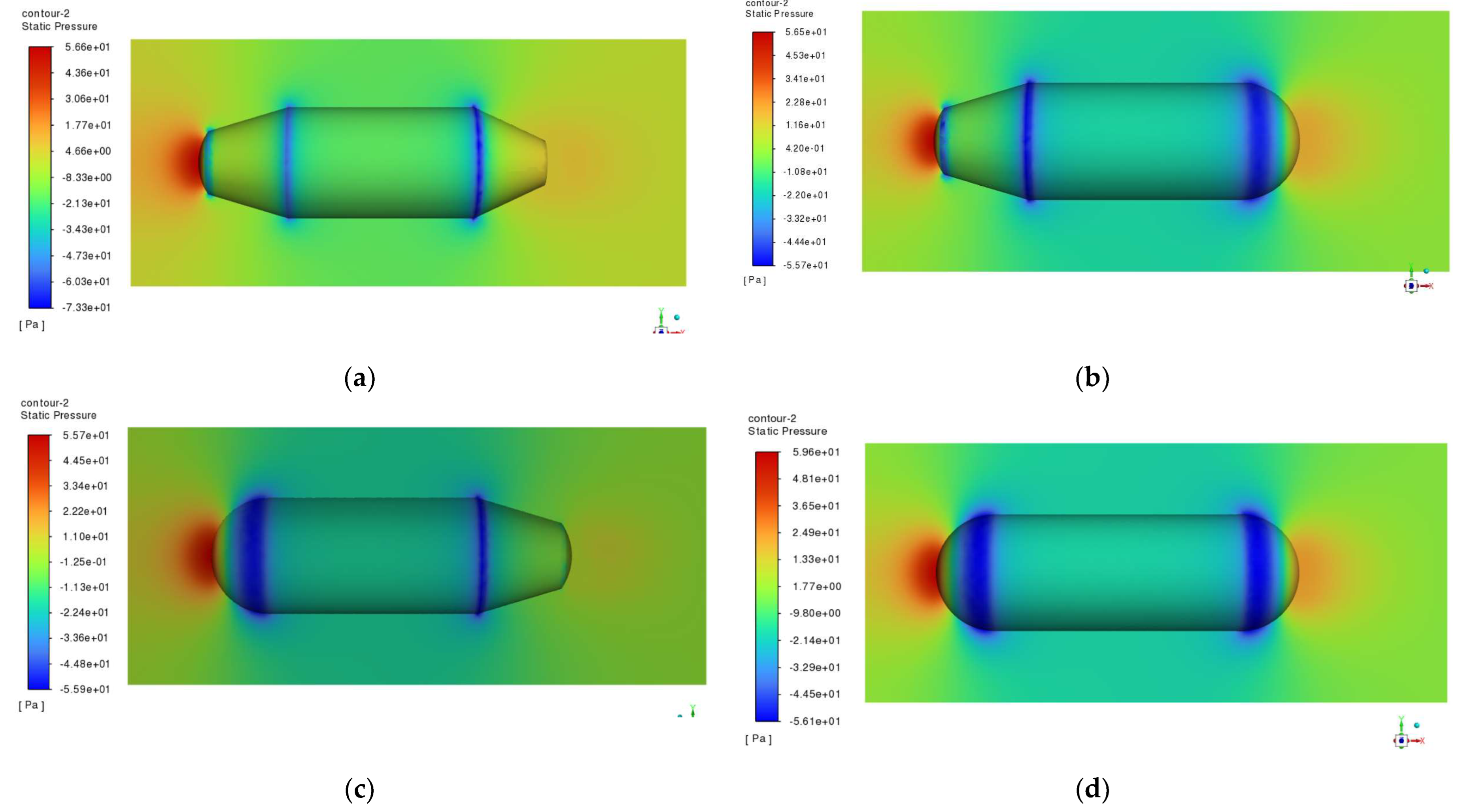
The flow field environment was simulated at a depth of 300 m, with a hydrostatic pressure of 3 MPa and a seawater flow velocity of 0.3 m/s. All simulation parameters were kept constant except for the structural variations among the models. Velocity and pressure distributions were generated for the four configurations.

As illustrated in Figure 5 and Figure 6, when the main float is subjected to current impact, the velocity at the upstream surface is zero, resulting in velocity concentration at the neck of the main float and stress concentration at its front section. The maximum velocities observed for the four models are 0.442 m/s, 0.428 m/s, 0.445 m/s, and 0.455 m/s, respectively. This phenomenon occurs because the current velocity decreases abruptly upon impacting the main structure, causing higher stress in the front region. As the flow extends along the streamlined body, the current eventually converges at the tail. The maximum hydrodynamic forces exerted on the main float are 56.6 Pa, 56.5 Pa, 55.7 Pa, and 59.6 Pa, respectively. In the pressure distribution diagram, the blue regions likely indicate low-pressure zones caused by flow separation on the float surface, which may contribute to increased drag forces.

Compared to a simple cylindrical structure, all four submerged buoy designs mitigate the effects of current impact and enhance the dynamic performance of the main float. Among these, Model IV, which features semicircular transitions at both ends, exhibits the highest flow resistance. Model II, with a streamlined transition at the front end, demonstrates the smallest flow velocity variation; however, its tapered design (narrow front and wide rear) makes it susceptible to turbulence-induced twisting. Model III, incorporating a semicircular transition at the front and a streamlined transition at the rear, represents the most optimal design. The spherical head design reduces fluid impact forces at the front, resulting in a more uniform stress distribution across the main structure and minimizing stress concentration. Additionally, the conical tail design facilitates flow convergence at the rear, reducing the likelihood of flow separation and mitigating the effects of trailing forces. Therefore, further simulation and structural optimization were conducted based on Model III.

3. Fluid Dynamics Simulation and Analysis of the Main Float

This study employs the RNG k-omega turbulence model, grounded in hydrodynamic theory, and the Navier-Stokes equations (N-S equations), based on the Reynolds-averaged simulation method, to simulate and analyze the pressure and velocity field distributions of the main float at a depth of 300 m. The governing equations of fluid dynamics comprise the continuity, momentum, and energy equations. Fluid motion follows the three conservation laws, which are the basis of fluid simulation and are used to describe the state of motion of a fluid.

The mass conservation equation describes the conservation of fluid mass:

$${\displaystyle \frac{\partial \rho }{\partial t}}+\nabla \cdot (\rho \mathbf{u})=0$$

(1)

where $\rho$ is the fluid density ($\mathrm{k}\mathrm{g}/\mathrm{m}³$); $\mathbf{u}$ is the velocity vector ($\mathrm{m}/\mathrm{s}$); $t$ is time ($\mathrm{s}$) and $\nabla$ is the dispersion operator.

The momentum conservation equation describes the change in fluid momentum:

$${\displaystyle \frac{\partial (\rho \mathbf{u})}{\partial t}}+\nabla \cdot (\rho \mathbf{u}\mathbf{u})=-\nabla p+\nabla \cdot \tau +\rho \mathbf{g}+\mathbf{f}$$

(2)

where $p$ is the pressure ($\mathrm{P}\mathrm{a}$); $\tau$ is the viscous stress tensor ($\mathrm{P}\mathrm{a}·\mathrm{s}$); $\mathbf{g}$ is the gravitational acceleration ($\mathrm{m}/\mathrm{s}²$); $\mathbf{f}$ is the external volume force (in this paper, the current impulse, $\mathrm{N}/\mathrm{m}³$).

For ocean currents, the viscous stress tensor τ can be expressed as follows:

$$\tau =\mu \left(\begin{array}{c}\nabla u+(\nabla u{)}^T\end{array}\right)-{\displaystyle \frac{2}{3}}\mu (\nabla \cdot \mathbf{u})\mathbf{I}$$

(3)

where $\mu$ is the dynamic viscosity ($\mathrm{P}\mathrm{a}·\mathrm{s}$); $\nabla \mathbf{u}$ is the velocity gradient tensor; $\mathbf{I}$ is the unit tensor; $\nabla \cdot \mathbf{u}$ is the dispersion of the velocity field, in this paper $\nabla \cdot \mathbf{u}\approx 0$.

The conservation of energy equation describes the change in fluid energy and provides a coupled solution mechanism of temperature-velocity-pressure field for the simulation, so that the simulation can capture the energy transformation in the high-speed flow:

$${\displaystyle \frac{\partial \left(\rho T\right)}{\partial t}}+{\displaystyle \frac{\partial \left(\rho uT\right)}{\partial x}}+{\displaystyle \frac{\partial \left(\rho vT\right)}{\partial y}}+{\displaystyle \frac{\partial \left(\rho wT\right)}{\partial z}}={\displaystyle \frac{\partial }{\partial x}}\left({\displaystyle \frac{k}{c_p}}{\displaystyle \frac{\partial T}{\partial x}}\right)+{\displaystyle \frac{\partial }{\partial y}}\left({\displaystyle \frac{k}{c_p}}{\displaystyle \frac{\partial T}{\partial y}}\right)+{\displaystyle \frac{\partial }{\partial z}}\left({\displaystyle \frac{k}{c_p}}{\displaystyle \frac{\partial T}{\partial z}}\right)+S_T$$

(4)

where $c_p$ is the specific heat capacity; $T$ is the temperature; $k$ is the heat transfer coefficient of the fluid, and $S_T$ is the internal heat source of the fluid and the portion of the fluid’s mechanical energy that is converted to heat due to viscous effects, sometimes referred to simply as $S_T$ for the viscous dissipation term.

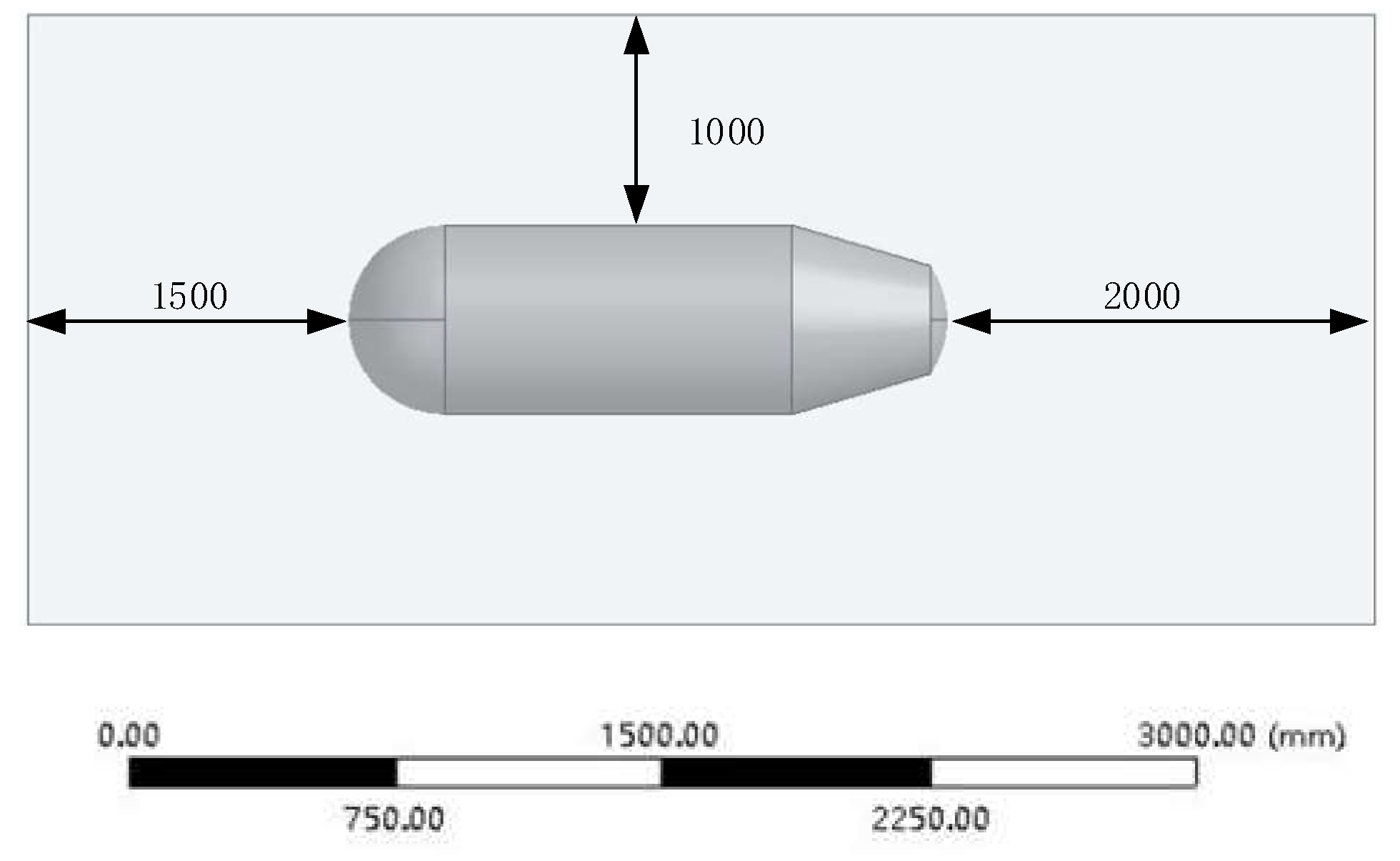
3.1. Simulation of Watershed Settings

After establishing the governing equations and selecting the turbulence model, the configuration of the simulation domain must be carefully designed. An undersized computational domain compromises flow field accuracy, whereas an excessively large domain results in unnecessary computational overhead. In this study, a rectangular simulation domain is adopted while ensuring its dimensions do not affect result validity. The seawater inlet is positioned at the front of the main float, with outlets distributed along all surrounding boundaries. The specific computational domain configuration is illustrated in Figure 7.

3.2. Grid-Independent Verification

Theoretically, higher mesh density in simulations enhances solution accuracy. However, practical applications reveal that excessive grid refinement significantly increases computational time costs. Beyond a critical threshold of grid elements, further mesh refinement yields diminishing returns in accuracy improvement. Therefore, this study prioritizes resource allocation to critical structural components and nodes before conducting precision simulations of the main floating body [17]. To validate grid independence, we implement the grid convergence criterion by progressively reducing grid scales until the residual tolerance $Re{s}_{\mathrm{s}\mathrm{p}\mathrm{a}\mathrm{c}\mathrm{e}}$ of time-averaged parameters stabilizes within the predefined threshold $e_s$.

$$Re{s}_{\mathrm{s}\mathrm{p}\mathrm{a}\mathrm{c}\mathrm{e}}=\left|{\displaystyle \frac{{\varphi }_{1 }-{\varphi }_{2 }}{{\varphi }_{1 }}}\right|\times 100\%⩽e_s,e_s\in \left(0.1\%\sim 0.5\%\right)$$

(5)

where ${\varphi }_{1 }$ is the lower grid target parameter (relative velocity magnitude in this paper) and ${\varphi }_{2 }$ is the upper grid target parameter. If $Re{s}_{\mathrm{s}\mathrm{p}\mathrm{a}\mathrm{c}\mathrm{e}}\le 0.5\%$, it is considered that the grid independence is established. Otherwise, it is necessary to continue to refine the grid. Firstly, the grid is initially divided into 500,000 cells, and then refined to approximately 1 million, 2 million, 3 million, and 4 million cells through volume refinement in the region near the main float. The differences in velocity diagrams around the main float are observed when water impacts it under five different grid resolutions. The corresponding velocity diagrams are shown below (Figure 8).

The relative velocities and $e_s$ of the main buoyant body head-on currents at different grid numbers are listed in

Table 1. Relative velocities and $e_s$ of main float under oncoming flow conditions.

Number	Number of Meshes	Number of Mesh Nodes	Velocity (m/s)	${\mathit{e}}_{\mathit{s}}$
1	517,961	143,438	0.394	—
2	945,609	248,390	0.392	0.51%
3	2,011,244	537,702	0.395	0.75%
4	3,096,555	868,628	0.394	0.25%
5	4,196,541	1,231,643	0.395	0.25%

, which is used for grid-independence validation.

It is verified that when the number of mesh cells reaches 3,096,555, the error in the velocity field solution between two consecutive time steps is within 0.5%. This indicates that increasing the number of mesh cells beyond 3,096,555 does not significantly improve computational accuracy. At this point, the influence of the grid on the results is within the acceptable range. The simulation grid is then used as a benchmark, and grid independence verification is completed. Considering computational time and simulation error, it can be approximated that grid independence is achieved when the number of mesh cells is around 3 million. Subsequently, the Ansys Fluent simulation of the main floating body is conducted using this benchmark grid.

3.3. Simulation of Seawater Flow Impact

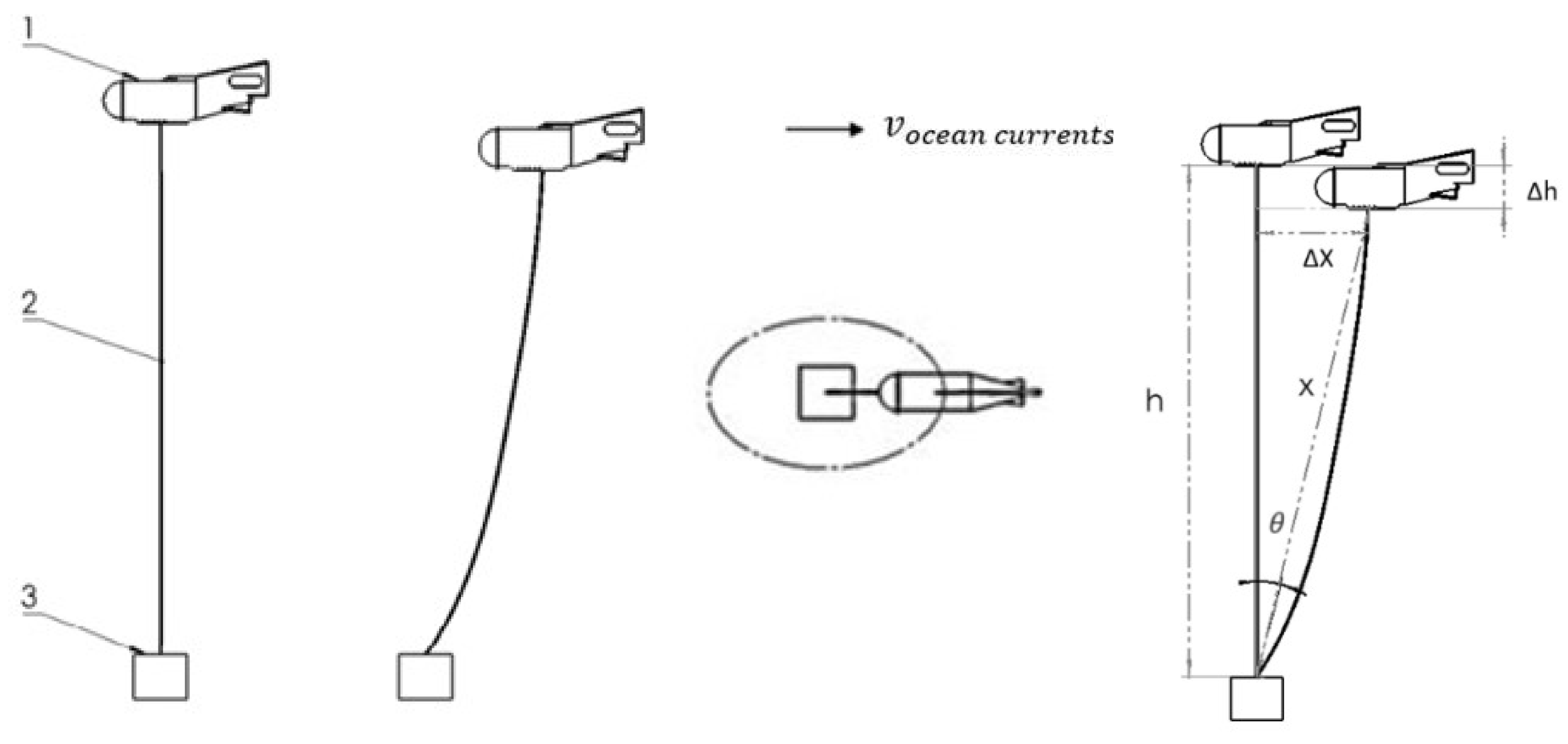
After the deployment of the submerged buoy, the main float is subjected to the combined effects of current impact, gravity anchor resistance, and buoyancy, causing the entire mooring system to undergo dynamic drift. In the deep-sea environment, the submerged buoy system experiences a horizontal offset of $∆X$ and a vertical displacement of $∆h$ in the direction of the mooring load, resulting in a deviation angle $\theta$ from the ideal vertical position. The current-induced trajectory of the buoy is approximately elliptical [18]. The submerged motion of the main float within the submerged buoy system is illustrated in the following Figure 9.

During this movement, the current impact has the greatest influence on the main float. A preliminary improvement to Model III can be achieved by adding a tail fin while maintaining the original bulbous head and streamlined transitional tail. The tail fin helps the main float align with the current, thereby reducing torsion and lateral motion [19]. The three-dimensional schematic of the main float with the added tail fin is shown in Figure 10.

Then, the frontal head-on current field simulation of the optimized submarine buoy main float is analyzed in Ansys Fluent. The main steps are as follows: import the above model, generate a shell as the flow field domain, divide the mesh into about 3 million, set the main float material (Al) and the flow field domain (water), set the current velocity (0.3 m/s) at the inlet of the flow field domain, use transient computation, and generate the relative velocity map and the pressure map of the main float subjected to the frontal impact of the current.

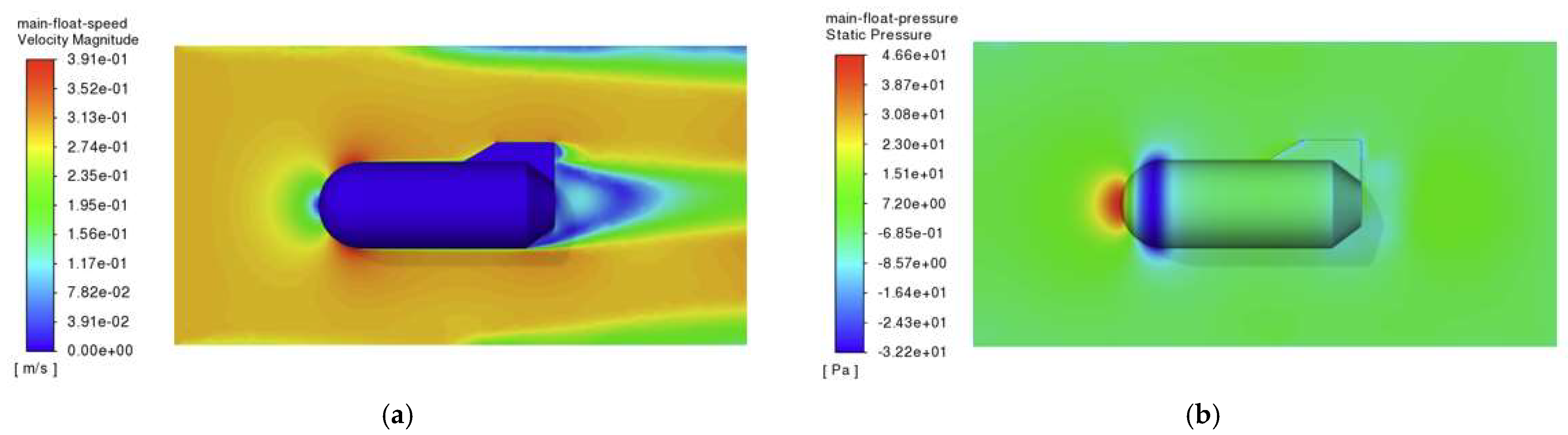
The relative velocity diagrams and flow pressure diagrams of the main float frontal subjected to the flow are shown in Figure 11.

As shown in the figure, the main float generates a relative velocity of 0.391 m/s when subjected to a head-on current of 0.3 m/s and experiences a flow pressure of 46.6 Pa. The addition of a tail fin enhances the infusion effect. Although increasing the tail fin enlarges the surface area of the main float, as long as the transition between the tail fin and the main float is smooth and the tail fin maintains good hydrodynamic streamlining, it does not generate significant resistance. After optimization, the flow remains smooth, and the wake region at the tail is significantly reduced. The maximum pressure caused by the current impact is also slightly reduced to 46.6 Pa, with the high-pressure area more evenly distributed and the negative-pressure vortex in the wake nearly eliminated. These improvements indicate that the structural stability of the main float is enhanced after the preliminary optimization of Model III.

3.4. Simulation of Multi-Angle Seawater Impact

The submerged buoy may also encounter turbulent currents at different angles during long-time underwater operation, which may cause a large displacement of the main float. To improve the torsional and transverse roll resistance of a submerged buoy and to reduce the dynamic behavior of the main float after being subjected to turbulence [20,21]. Next, the simulation test of the main float impacted by multi-angle currents is carried out to observe whether the new main float structure can have better stability under the impact of lateral currents (taking 30° and 45° as an example). Evaluate the dynamic response and force on the float when it is impacted by currents at different angles. Generate simulation plots of the relative velocities and pressures subjected to the flow in the side-on currents of the main float (top and side views), as shown in Figure 12 and Figure 13.

As shown in the figure, when the main float is subjected to lateral incoming flow, it generates a higher relative velocity compared to head-on flow, and the side of the main float experiences a greater pressure impact [22]. This is likely to cause twisting or swaying, leading to instability. Therefore, to reduce the dynamic response of the main float in turbulent conditions, its structure is further optimized while maintaining the original dimensions. A central slot is cut into the main float to accommodate an underwater winch for real-time data transmission. Additionally, a slot is introduced in the tail fin to allow lateral currents to pass through, and symmetrical tail fins are added on both sides to enhance the float’s anti-roll capability. The optimized main float structure is shown in the figure below (Figure 14).

The optimized main float is re-simulated and compared with the previous structure to evaluate improvements in its hydrodynamic performance [23]. As shown in Figure 15 and Figure 16.

The 30° lateral current impingement was analyzed. Before optimization, the maximum velocity of the main buoy in the region of the tail vortex was 0.47 m/s, which formed a Karman vortex street [24], indicating severe flow separation. After the introduction of the tail-fin notch design, the lateral incoming flow was guided into the notch, forming a fluid path. This control strategy effectively disrupts the coherent structure of the vortex, destroys the large-scale vortex street, and breaks up the wake vortex into smaller-scale turbulence, resulting in a reduction of about 40% of the reverse flow area. The maximum velocity is reduced to 0.421 m/s, and the wake high-velocity region is reduced, resulting in a reduction of pressure drag.

Before optimization, the peak pressure on the main buoy was 45.2 Pa, concentrated at the center of the inflow surface. After optimization, the channeling effect of the optimized slot increased the peak pressure to 49.1 Pa, but the location of the effect was extended towards the caudal fin, creating a more uniform pressure distribution. This indicates that the slot disperses the leading edge loads, and the accelerated flow in the slots leads to an increase in the local Reynolds number and a reduction in the differential pressure resistance, resulting in a smoother pressure gradient. The dual tail design extends the flow attachment area, reduces tail flow separation, further reduces drag, balances lateral separation forces, and suppresses transverse and longitudinal rocking motions.

The relative velocity of the main float subjected to flow also decreased from 0.461 m/s to 0.429 m/s under the impact of 45° lateral current, and the peak pressure subjected to flow increased from 45.6 Pa to 47 Pa, which indicated that the notch deflector on the caudal fin could maintain its effectiveness in the incoming flow at a larger angle.

Based on these findings, it can be concluded that the synergistic optimization of the tail fin slot and the double tail fins significantly improves the hydrodynamic performance of the main buoy under lateral current impact and enhances its stability.

4. Flow-Induced Noise Simulation of the Main Buoy Body

Due to the superior propagation characteristics of low-frequency, high-power acoustic waves in seawater, the submerged buoy system is equipped with acoustic hydrophones for underwater anomalous acoustic monitoring. Mainly used for military monitoring and early warning, monitoring ships, submarines, submersibles, and so on. The detection frequency is mainly concentrated within the 1 kHz band. However, when detecting long-range signals, the detection performance of acoustic hydrophones can be compromised by flow-induced vibration noise and electrical noise. Most existing acoustic buoy platforms often overlook the interference caused by self-vibration and inherent noise of the buoy structure under external environmental forces during their development, which exerts a non-negligible impact on the monitoring accuracy and sensitivity of acoustic hydrophones. The mitigation of noise interference during hydrophone operation remains a critical research focus [25]. In this paper, the submerged buoy system adopts a serrated protection frame to carry the hydrophone, and according to the existing related literature, the serrated protection frame can effectively reduce the current noise of the hydrophone [26], but the main float is large in size, and the current will generate large current noise after impacting the main float. This streaming noise component has an effect on the hydrophone. Under normal operating conditions in the ocean, this flow noise will be significantly larger than the ocean ambient noise. To address these challenges, this study integrates hydrodynamic principles to conduct vibration and noise analysis based on multidimensional coupling. COMSOL Multiphysics is employed to simulate flow-induced noise generated by ocean current impacts on the main buoy body, with subsequent analysis of spatial distribution patterns and decibel levels in the radiated acoustic field. Study the theory of maximum current noise generated by the sea current impacting the main float. And arrange the hydrophone at the position of the main float after the attenuation of the current noise, which can effectively avoid the influence of the current noise generated by the current impacting the main float, and improve the quality of the hydrophone monitoring data.

The traditional method of calculating the flow noise can use the LES+FW-H equation, but since this method requires the division of a high-resolution grid, it leads to excessive computation and high computational cost, which often leads to errors in the simulation results [27]. In this paper, we first use Ansys Fluent to perform the fluid-solid coupling simulation to get the main floating body subjected to the flow impulse, and then use COMSOL Multiphysics to perform the acoustic-solid coupling simulation by directly applying a plane wave excitation of the same size. Compared with the conventional method, the simulation is all about the impact-induced vibration of the structure, which in turn causes the noise. In this paper, the method of flow-solid coupling followed by acoustic-solid coupling will greatly reduce the amount of single calculation, and the accurate flow noise magnitude can be obtained with less calculation.

The flow-induced vibration noise simulation method used in this paper first requires obtaining the water flow force simulated by Ansys Fluent [28]. After convection processing, the effect of the flow on the main buoyancy system is equivalent to the effect of water flow resistance.

$$R={\displaystyle \frac{1}{2}}\rho C_{D}A{V}^2$$

(6)

where $R$ represents the hydrodynamic resistance; $C_D$ denotes the normal drag coefficient (dimensionless); $A$ corresponds to the frontal area of the object (${\mathrm{m}}^2$); $V$ signifies the relative velocity between the object and fluid ($\mathrm{m}/\mathrm{s}$).

However, since the hydrodynamic load inherently acts on curved surfaces (specifically the inflow surface of the submerged buoy system), whereas the equivalent hydrodynamic resistance is simplified as a point force, the force is subsequently converted into planar wave excitation parallel to the simulation inlet. This methodology transforms the hydrodynamic impact on the main buoy into planar wave excitation, enabling the simulation of flow-induced noise through structural vibration analysis under planar wave excitation. Since this paper requires the calculation of the maximum flow noise that can be generated by the main buoyancy body, we have selected the characteristic peak value of pulsating pressure in fluid-structure interaction simulation as the plane wave excitation, with the aim of quantifying the equivalent excitation amplitude that can effectively excite structural vibrations. Compared to conventional flow-induced noise simulations that require a comprehensive consideration of acoustic propagation characteristics in seawater, the planar wave assumption significantly reduces computational complexity. For low-frequency noise monitored by acoustic hydrophones, the planar wave assumption is generally acceptable.

Further, the main buoyancy body is treated as an elastic medium. Fluid loads are generated at the fluid-structure interface, while the acoustic-structure interface also imposes elastic stresses on the structural body. In this paper, turbulent waves are considered as acoustic source terms, and the generation and propagation of the acoustic field are separated using the wave equation. By combining the fluid wave equation and the structural dynamics equation, the displacement and sound pressure on the elastic structural surface can be calculated [29]. The flow-induced vibration noise simulation method used in this paper first requires obtaining the fluid flow force simulated by Ansys Fluent. After convective processing, the effect of the flow on the main buoyancy system is equivalent to the effect of fluid resistance. For acoustic wave equations:

$$\nabla \left({\displaystyle \frac{1}{\rho }}\nabla p\right)+{\displaystyle \frac{k^2}{\rho }}p=0$$

(7)

Applying its variational form:

$${\int }_{{\Omega }_f} \left[-{\displaystyle \frac{1}{{\omega }^2{\rho }_f}}\nabla p\cdot \delta (\nabla p)+{\displaystyle \frac{1}{{\rho }_f{c}^2}}p\delta p\right]\mathrm{d}\Omega +{\int }_{\partial \Omega } {\displaystyle \frac{1}{{\omega }^2{\rho }_f}}\nabla p\cdot \mathit{n}\delta p\mathrm{d}S=0$$

(8)

where $p$ is sound pressure; ${\rho }_f$ is background medium density; $c$ is sound velocity and $\omega$ is angular frequency.

Considering that the acoustic pressure within the field satisfies the superposition of incident and scattered acoustic fields, we obtain the following equation:

$$p=p_{\mathrm{s}\mathrm{c}\mathrm{a}\mathrm{t}}+p_{\mathrm{i}\mathrm{n}\mathrm{c}}$$

(9)

Which can be substituted into the following:

$$\begin{array}{c}{\int }_{{\Omega }_f}[-{\displaystyle \frac{1}{{\omega }^2{\rho }_f}}\nabla p_{\mathrm{sact} }\cdot \delta (\nabla p_{\mathrm{s}\mathrm{c}\mathrm{a}\mathrm{t}})+{\displaystyle \frac{1}{{\rho }_f{c}^2}}{p}_{\mathrm{sact} }\delta p_{\mathrm{sact} }]·\mathrm{d}\Omega \\ +{\int }_{\partial \Omega }{\displaystyle \frac{1}{{\omega }^2{\rho }_f}}\nabla p_{\mathrm{s}\mathrm{c}\mathrm{a}\mathrm{t}}\cdot \mathit{n}\delta p_{\mathrm{sact} }\mathrm{d}S=0\end{array}$$

(10)

For isotropic homogeneous linear elastic bodies, the structural governing equation can be expressed as follows:

$${\int }_{{\Omega }_s}(-{\omega }^2{\rho }_s{x}_i\delta x_i+{\sigma }_{ij}\delta {\epsilon }_{ij})\mathrm{d}\Omega -{\int }_{\partial \Omega }{t}_i\delta x_{i}dS=0$$

(11)

where $i,j=\mathrm{1,2},\dots$; ${\rho }_s$ denotes material density; $x_i$ represents displacement magnitude components of the elastic body; ${\epsilon }_{ij}={\displaystyle \frac{1}{2}}\left({\displaystyle \frac{\partial u_i}{\partial x_j}}+{\displaystyle \frac{\partial u_j}{\partial x_i}}\right)$ defines the strain tensor; ${\sigma }_{ij}=C_m{\epsilon }_{ml}$ expresses the elastic constitutive relationship, where $C_m$ is the damping matrix of the elastic material; $t_i={\sigma }_{ij}{n}_j$ indicates boundary traction forces. The acoustic-structure coupling problem can be considered as a generalized fluid-structure interaction problem. The boundary conditions adopt normal stress and acoustic pressure continuity conditions: ${\sigma }_{ij}=p{\delta }_{ij}$. Following the principle of virtual work, the interfacial forces can be equivalently transformed into nodal forces acting on finite elements. Consequently, the coupled vibration equation is formulated as follows:

$$\left[\begin{array}{cc}{\mathit{M}}_s& 0\\ {\rho }_f& {\mathit{M}}_f\end{array}\right]\left\{\begin{array}{c}\ddot{U}\\ \ddot{P}\end{array}\right\}+\left[\begin{array}{cc}{\mathit{C}}_m& 0\\ 0& {\mathit{C}}_f\end{array}\right]\left\{\begin{array}{c}\dot{U}\\ \dot{P}\end{array}\right\}+\left[\begin{array}{cc}{\mathit{K}}_s& -{\mathit{R}}^{\mathrm{T}}\\ 0& {\mathit{K}}_f\end{array}\right]\left\{\begin{array}{c}\mathit{U}\\ \mathit{P}\end{array}\right\}=\left\{\begin{array}{c}{F}_S\\ 0\end{array}\right\}$$

(12)

where ${\mathit{M}}_s$, ${\mathit{C}}_m$, and ${\mathit{K}}_s$ represent the mass, damping, and stiffness matrices of the elastic body, respectively; ${\mathit{M}}_f$, ${\mathit{C}}_f$, and ${\mathit{K}}_f$ denote the mass, damping, and stiffness matrices of the adjacent fluid domain, respectively; $\mathit{R}$ is the coupling matrix characterizing interface interactions; $\mathit{U}$ and $\mathit{P}$ correspond to the displacement, velocity, and acceleration vectors at the element nodes; $F_S$ signifies the external loading vector.

In this paper, the turbulent fluctuations are regarded as sound source terms, and the sound field generation and propagation processes are separated by fluctuation equations [30]. The spectrum of turbulent fluctuations is estimated by empirical equations, and the energy spectrum is extracted from the transient velocity field by obtaining the flow field data (velocity $u_i$, pressure $p$, density $\rho$) using the previous fluid simulation:

$$E(k)={\sum }_{k\le \mathbf{k}\mid <k+\mathsf{\Delta }k}{\displaystyle \frac{1}{2}}|\hat{\overline{u}}(\mathbf{k}){|}^2$$

(13)

Further use of the separation of the turbulent source term from the acoustic propagation process using the Lighthill equation, considering turbulent fluctuations as sound source terms, the Lighthill stress tensor is constructed as follows:

$$T_{ij}=\rho u_i{u}_j+\left(p-c^2\rho \right){\delta }_{ij}-{\tau }_{ij}$$

(14)

The sound propagation equation is as follows:

$${\displaystyle \frac{{\partial }^2{\rho }^{\prime }}{\partial t^2}}-c^2{\nabla }^2{\rho }^{\prime }={\displaystyle \frac{{\partial }^2{T}_{ij}}{\partial x_i\partial x_j}}$$

(15)

where: $T_{ij}$ is the Lighthill stress tensor; $u_i{,u}_j$ refers to the component of the velocity vector in the i, j direction (m/s); ${\tau }_{ij}$ is the viscous stress tensor; $\rho u_i{u}_j$ is the Reynolds stress term; $(p-c^2\rho ){\delta }_{ij}$ is the compressive stress term; $c$ is the background medium sound velocity; ${\rho }^{\prime }=\rho -{\rho }_0$ is the density perturbation (${\rho }_0$ is the background density).

The acoustic pressure field $S$ is solved by substituting $T_{ij}$ as a source term into the fluctuation equation based on the Green’s function of the fluctuation equation.

$$S={\displaystyle \frac{1}{4\pi c_0^2}}{\int }_V {\displaystyle \frac{{\partial }^2{T}_{ij}}{\partial y_i\partial y_j}}{\displaystyle \frac{1}{|\mathbf{x}-\mathbf{y}|}}\delta \left(t-{\displaystyle \frac{|\mathbf{x}-\mathbf{y}|}{c_0}}\right)d^3\mathrm{y}$$

(16)

The vibration noise solution process is shown in the figure below (Figure 17).

Flow-induced noise simulations of the main buoy are conducted in COMSOL Multiphysics. The Pressure Acoustics module is employed to model pressure waves generated by hydrodynamic impacts [31]. Entering analog pressure as a known variable directly into COMSOL settings, select a pressure of 46.6 Pa on the front-facing flow of the main float, definite computational and acoustic domains, and propagate fluid pressure fluctuations to the acoustic domain (In this paper, the pressure of 46.6 Pa is used as an example, and this method can also be used to calculate the noise of the main float subjected to currents at different angles). Subsequently, the Solid Mechanics module is coupled to resolve acoustic-structure interactions. We used frequency domain calculations in our study, which ultimately allowed us to characterize the sound pressure level (SPL) distribution around the main buoy structure.

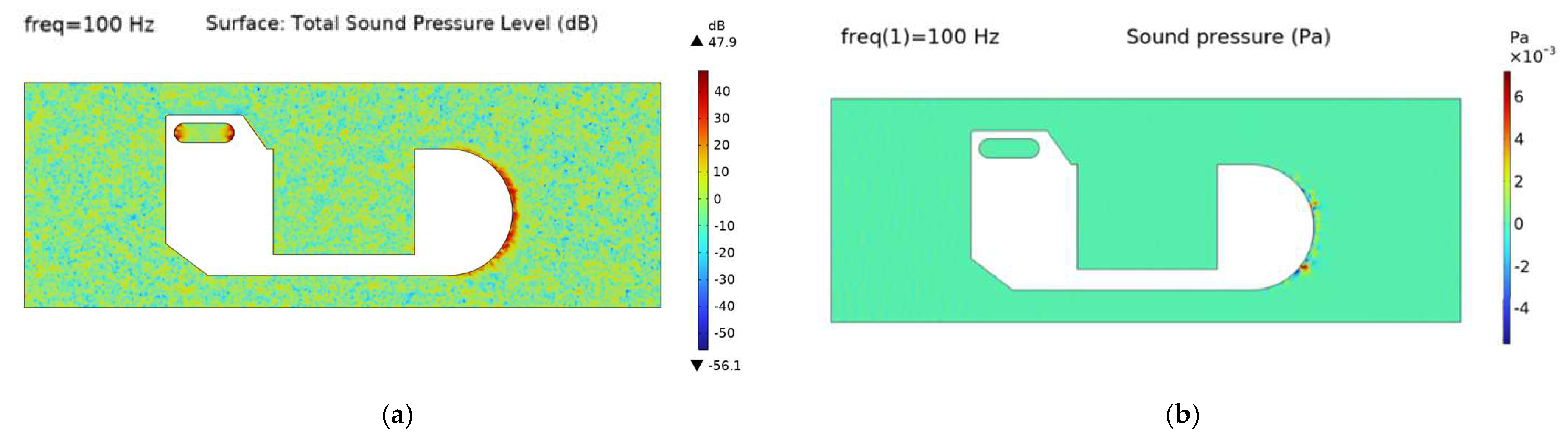
Specific steps are importing a geometric model—stretching the work plane to form a union as a simulation domain (1600 mm × 2000 mm × 4500 mm)—setting the main floating body material (Al) and the simulation domain (water)—increase the pressure acoustic frequency domain and solid mechanics module (according to the fluid simulation of the numerical input)—mesh delineation—frequency domain calculations—steady state solutions. Generate the total sound pressure level and total sound pressure diagram of the main float vibration noise, as shown in Figure 18.

Flow-induced noise simulations of the main buoy demonstrate spatially heterogeneous energy distribution characteristics. The flow-induced noise predominantly concentrates within 0.5 m from the buoy surface, exhibiting exponential attenuation of sound pressure level (SPL). Beyond 1.2 m from the structure, the flow noise attenuates to ambient background levels (10–20 dB). Maximum noise peaks reaching 47.856 dB occur at the hydrodynamic stagnation point, showing strong agreement with predictions from classical cylindrical flow noise theory (40~60 dB) [32]. We further referenced the work of Wang Kang et al., who studied the flow noise characteristics of underwater vehicles using the LES method and Lighthill acoustic analogy theory. The volume of the vehicle model is similar to that of the main buoy body studied in this paper. They found that at low speeds, the hydrodynamic flow noise excited by the hull is the primary noise source, and the noise increases with the vehicle’s speed, ranging from 45 dB to 52 dB [33]. The main buoy body of the mooring studied in this paper can be regarded as an underwater vehicle with a speed of 0, and the flow noise should be around 45 dB. This is similar to the flow noise calculation result of 47.856 dB in this paper, within a reasonable error range. Hydrophone deployment in the acoustic shadow zone beyond 1.5 m from the main buoy can effectively mitigate flow-induced noise interference.

5. Conclusions

This study investigates a novel acoustic submerged buoy’s main float based on hydrodynamic theory, designed for long-term underwater target early-warning monitoring. Through fluid-structure interaction simulations, the deep-sea dynamic response is analyzed by calculating velocity and pressure field distributions around the main float. Structural optimization effectively enhances its attitude stability. A new vibration-induced noise calculation methodology is proposed, employing planar wave excitation to simulate hydrodynamic impacts. Under 300-m deep-sea conditions, the main float subjected to 0.3 m/s current flow generates 47.856 dB noise, providing precise ambient baseline noise data for acoustic monitoring instruments. The research establishes theoretical foundations and technical references for optimizing buoy float configurations and controlling flow-induced vibrations, thereby improving detection system accuracy and reliability.

However, this paper lacks relevant experimental verification of the simulation and only uses the conclusions of other researchers to preliminarily prove the effectiveness of the simulation. Furthermore, the simulation method used in this paper is more suitable for the conceptual design stage of acoustic buoys, with the aim of optimizing the main buoy structure and roughly calculating the flow noise generated by the main buoy. It is a novel method that balances computational efficiency and accuracy, but it cannot achieve high-precision measurement of vibration noise. In the next step, we will actively seek experimental data for final verification. After testing all the functions of the main buoy, the next step will be to conduct sea trials in the South China Sea to validate the main buoy’s performance and expand its application range. The main validation plan is as follows:

(1)

A 3 × 3 high-dynamic pressure sensor array is deployed on the upstream surface of the main buoyancy body to measure the impact force of underwater turbulence, recording the time-history curve of turbulent pulsation pressure, and comparing the pressure peak values with simulation data.

(2)

Utilize the attitude sensors (IMU) mounted on the main buoy to evaluate its fluid performance, assessing its roll and pitch angles.

(3)

Place hydrophones inside the main buoy to measure the noise generated by turbulent impacts after the buoy stabilizes, and compare the results with the simulation data presented in this paper.