A Reef’s High-Frequency Soundscape and the Effect on Telemetry Efforts: A Biotic and Abiotic Balance

Abstract

Acoustic telemetry is a tool for tracking animals, but transmitted signals from tagged animals are not always detected. Detection efficiency declines with increasing background noise, which can have both abiotic and biotic sources. The abiotic noise present in reef environments (waves, bubbles, etc.) is primarily low-frequency, but snapping shrimp create high-frequency noise that can interfere with transmission detections. Prior work in shallow coastal reefs correlated winds with less high-frequency background noise, and hypothesized that it was due to a balance of biotic and/or abiotic factors: shrimp may be less active during high wind events, and sound attenuation at the surface increases with wave height. To test this hypothesis, passive acoustic recordings from a live-bottom reef are used to quantify snapping shrimp snap rate. Snap rate was strongly correlated with temperature, and warmer environments appeared to be challenging for acoustic telemetry. However, the majority of synoptic variability in noise is shown to be driven by abiotic attenuation. Wind speed has little to no effect on snapping shrimp behavior, but has a significant inverse correlation with high-frequency noise levels due to surface attenuation of high-frequency noise, and therefore a positive effect on detection efficiency, pointing to primarily abiotic forcing behind noise variability and resulting telemetry success. This research gives context to previously collected detection data and can be leveraged to help plan future acoustic arrays in shallow, complex, and/or noisy environments, potentially predicting changes in detection range.

1. Introduction

Acoustic telemetry, “tagging” species of interest by implanting small transmitters and using receivers to detect these high-frequency signals, is a popular research tool for tracking marine animals, but the probability of detecting these signals heavily depends on the environment [1,2,3]. A lack of detections can mistakenly be considered an absence of transmissions to detect, when in reality a transmission may have been present but the receiver failed to detect it [1,2,4]. Acoustic telemetry detection efficiency is expected to decrease with distance [5], especially in shallow coastal environments [6], but changes in the physical environment can also directly influence transmission detection [2,7,8]. Consequently, environment-specific range testing is an important part of estimating dynamic detection probability and range [9]. Understanding the processes that determine how far transmissions travel is a fundamental part of the design of acoustic arrays [10].

Shallow coastal waters affect how sounds travel, and these environments are often characterized by strong spatial and temporal variability of water column properties [11] that can change detection efficiency [6]. The speed of sound is dependent on the physical properties of the water column (temperature, salinity, pressure) and the sound speed profile (SSP) dictates how signals travel [12]; these profiles can vary rapidly in shallow water columns affected by both top and bottom boundary layers [6]. The rate at which sound travels and attenuates depends on the sound frequency and environmental conditions [13]. Sound bends and refracts away from local sound speed maxima, which depend on temperature and salinity, so stratified environments often result in more heterogeneous soundscapes [6,12]. Most of the attenuation in shallow (<20 m) environments involves at least one boundary layer and winds increase sound attenuation at the air–sea interface [14]. Wind-driven white caps and waves create turbulence and bubble plumes that result in an asymmetric effect on background noise at different frequencies: the wind creates large amounts of low-frequency noise through wave breaking and turbulence [15,16], while attenuating high-frequency noise at a higher rate and limiting surface reflectance [17,18].

One of the most important factors in telemetry efficiency is local background noise; sounds at similar frequencies can interfere with detections by masking the transmissions [1,19]. Live-bottom coastal reefs are expected to be acoustically challenging soundscapes due to both abiotic (wind, waves, bubbles) and biotic (fish, snapping shrimp, etc.) sources of background noise [20,21]. Waves, storms, and bubbles create low-frequency (<20 kHz) noise [17], with very little overlap with the frequencies commonly used in acoustic telemetry (50–90 kHz) [22]. Snapping shrimp are of specific concern for interference due to the broadband (0.2–200 kHz) nature of their snaps, made when their claws form and pop a cavitation bubble that creates a powerful and consistent sound that is one of the few common biotic sources of noise at higher frequencies (>50 kHz) [23,24]. The rate of snapping varies over predictable time scales: seasonal signals in which warming increases snaps [21], and diel cycles over which shrimp are expected to be more active at sunset and during the night [23].

Ambient noise near the transmission frequency band can limit detection efficiency [1], so snapping shrimp activity should concern researchers using telemetry techniques. Studying environments where snapping shrimp are present requires accounting for their behavior: more detections are expected when snapping shrimp are less active due to decreased noise interference [3], an issue cited by the manufacturer [25]. Estimation of background noise and telemetry efficiency could be critical for providing context and interpretation for collected detection data [3].

This research explores a previously noted positive relationship between wind speed and detection efficiency on a shallow, noisy reef [3], for which the underlying mechanism was not identified. A biotic explanation would be that snapping shrimp are less active during high winds, creating less noise and lowering interference, increasing the number of successful detections (Figure 1A) [26]. A competing abiotic explanation is that benthic activity is not affected by the increased winds and the same amount of noise is being created, but increased surface attenuation enables telemetry efforts by lowering background noise (Figure 1B) [14]. Wind appears to be an important factor in telemetry efficiency in a variety of environments [3,18,27], and understanding the mechanism would add context to collected detection data.

We hypothesize that high winds result in less noise created by lowering shrimp activity and increasing surface attenuation, both contributing to a quieter, more optimal environment for acoustic telemetry that results in higher detection efficiency. We expect decreased snap rates during periods of high winds, and a higher rate of noise attenuated at the surface, accounting for both biotic and abiotic factors in the soundscape variability. If defined, this relationship would be a practical way to use atmospheric and buoy wave data to inform acoustic studies and detection ranges in these biologically important but acoustically challenging environments.

The following research tests our hypothesis for why telemetry efforts are more successful as winds increase (changes in snapping shrimp behavior and increased surface attenuation). Section 2.1 describes the experimental region and data collection methods, detailing the instruments and data formats. Section 2.3 explains how snapping shrimp behavior is estimated from passive acoustic data to quantify high-frequency noise creation, and Section 2.4 describes the method for quantifying noise attenuation by calculating surface bubble loss. In Section 3, detection data from moored transceivers are compared to the noise created and noise lost during high winds to explore the mechanism behind the increased detection success. Section 4 breaks down the findings and significance of the outcomes, and presents some ways to account for this relationship.

2. Materials and Methods

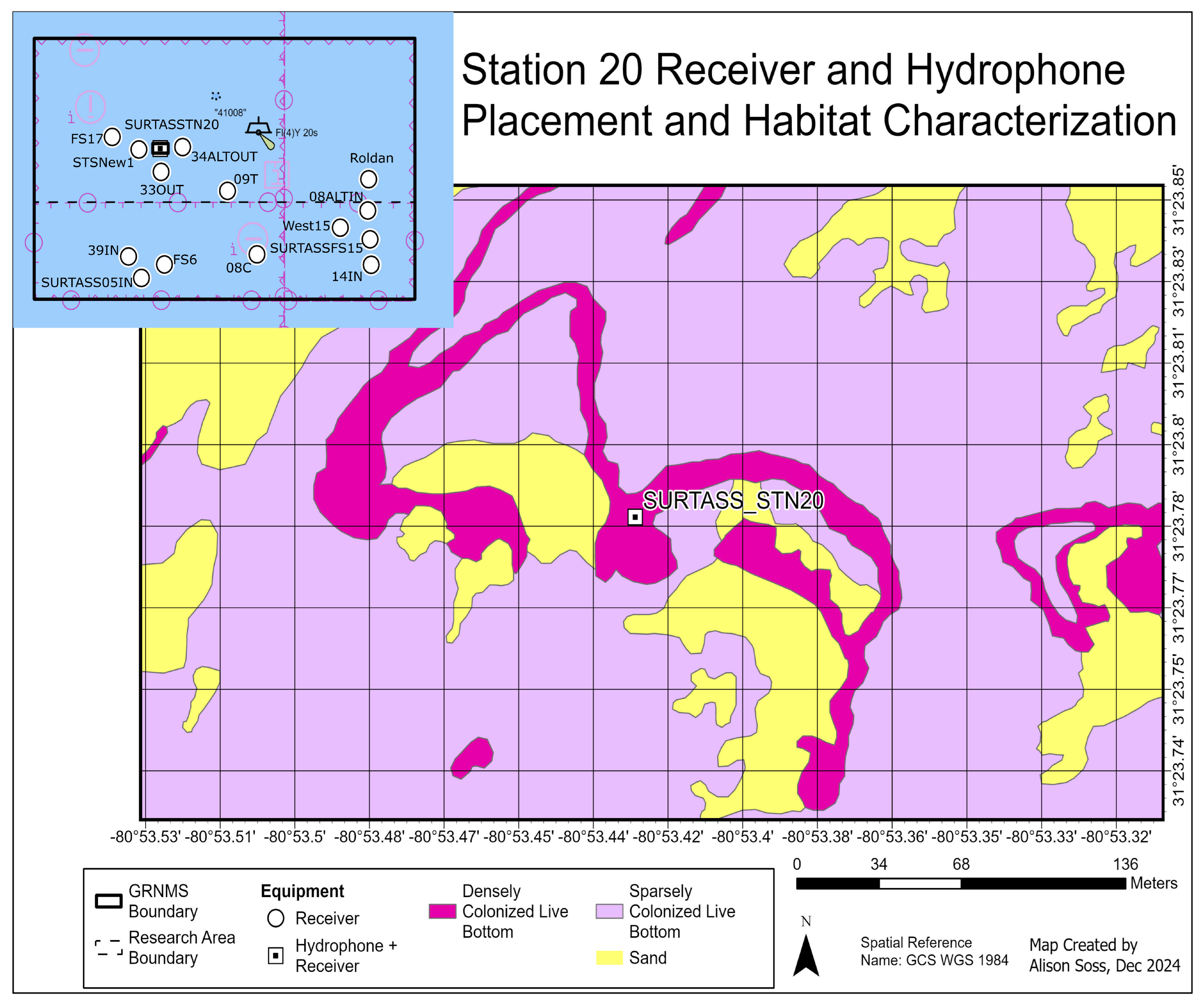
2.1. Environmental Context

Gray’s Reef National Marine Sanctuary (GRNMS) is a live-bottom reef off the coast of the southeastern United States on the South Atlantic Bight (SAB), which is a broad shelf influenced by the Gulf Stream and the discharge of freshwater rivers closer to shore (Figure 2) [11]. GRNMS lies along the 20 m isobath and provides habitat for more than 200 species of fish and invertebrates including snapping shrimp [21,28].

National Data Buoy Center (NDBC) Station 41008 measures significant wave height (m, highest one-third of all the waves during 20 min sampling), sea surface temperature (SST, °C, 2 m below the surface), and wind speed (m/s, averaged over an 8 min period) at GRNMS (31°24′0″ N, 80°51′59″ W) (

Table 1. Overview of instrumentation and data. Bottom temperature, detections, noise, and snap rate ranges are from SURTASSTN20.

	Units	Source	Range	Usage
Bottom Temp.	°C	VR2Tx	13.5–21.5	Env. context
Detections	detections/h	VR2Tx	0–8	Telemetry efficiency
High-Freq. Noise	mV	VR2Tx	400–769	Background noise (50–90 kHz)
Low-Freq. Noise	dB re 1 $\mathsf{\mu }$ Pa	SoundTrap 500	74–116	Background noise (0.17–0.36 kHz)
Snaps	snaps/h	SoundTrap 500	171–6758	Noise creation
SST	°C	NDBC Station 41008	12.6–23.7	Env. context
Surface Bubble Loss (SBL)	dB	Calculated	0.2–15	Noise attenuation
Thermal Stratification	$\Delta$°C	VR2Tx, NDBC	0–6.5	Env. context
Wave Height	m	NDBC Station 41008	0–2.87	Env. context
Wind Speed	m/s	NDBC Station 41008	0.2–14.3	Env. context

). Missing data (115 h out of 8784, <2%), none of which were subsequent, were linearly interpolated in time. Wind events were defined as periods with 2 or more days of sustained strong (>8 m/s) winds, including several hours before and after to isolate the possible effects of the wind event. We assume that horizontal stratification, which changes seasonally on the inner shelf near GRNMS [29], was small within Gray’s Reef itself. For the purposes of this research, we assume that data collected at the sea surface were representative of the entire sanctuary.

During the evaluation period, autonomous underwater vehicles (AUVs, gliders; Teledyne Webb Research, North Falmouth, MA, USA) were deployed to profile the water column for three separate missions totaling 88 days measuring conductivity, temperature, and pressure with a pumped GPCTD (Sea-Bird Electronics, Bellevue, WA, USA) as it dived and climbed at a 26° angle to support the SURTASS Soundscapes program, designed to create best practices in acoustic monitoring programs for marine-protected areas (Table 1) [21]. Data were processed to remove data points before and after deployment, then bin-averaged to 1 h and 1 m resolutions. Bulk thermal and density stratification measurements are estimated as the differences between the minimum and maximum from each binned hour to quantify vertical changes.

2.2. Telemetry Detections and Acoustic Measurements

Thirteen VR2Tx transceivers (Innovasea, Bedford, NS, Canada) were moored at GRNMS between November 2019 and December 2020, with water depths ranging from 14 to 21 m and spread apart so that the nearest receiver was between 400 and 1400 m away (Figure 2). Each transceiver sent and received low-power (142 dB) transmissions, and reported background noise (50–90 kHz, measured 6 times per hour then averaged as an hourly value) and temperature (°C, once per hour). The transmissions themselves are a short (3 s) series of 8–10 high-frequency (69 kHz) pings, with the timing between pings identifying the unique transmitter [30]. The transmitter IDs for the transceivers moored at GRNMS (Figure 2) were known a priori, as were the serial numbers implanted in six black sea bass tagged by GRNMS partners in 2019; unknown tags were assumed to come from fish tagged outside Gray’s Reef. The majority (>98%) of total detections in the array were from the identified VR2Tx transceivers, with a small number of detections originated from tagged fish. The transceivers were programmed to transmit once every 540–660 s, offset from each other to avoid collisions. Six transceiver detections per hour is considered 100% efficiency between two specific VR2Tx instruments, but some transceivers may receive more due to the offset. Reported detection efficiency was calculated between two instruments assuming a maximum of 6 detections per hour.

Acoustic data analyzed for this research were collected and quantified from two different datasets: high-frequency noise measured by VR2Tx transceivers, and continuous low-frequency hydrophone recordings (Table 1). High-frequency noise measured in the 50–90 kHz band by VR2Tx transceivers was an hourly average of the background noise measured (in millivolts, mV) once per minute across a relatively broad frequency band. This measurement was designed so that telemetry users could estimate possible noise interference in the transmission frequency band. Converting the VR2Tx transceiver’s millivolt measurements to a unit like sound pressure levels (e.g., dB re 1 $\mathsf{\mu }$ Pa) would inject large amounts of uncertainty due to the broad frequency band (pers. comm. with Innovasea), so we chose to use the manufacturer’s measurement in mV as prescribed. The transmissions were included in the transceiver’s noise measurements but were considered negligible with respect to external sources. Low-frequency (0.2–24 kHz) sound recordings were collected by a SoundTrap 500 hydrophone (Ocean Instruments, San Diego, CA, USA) moored 1 m off the live-bottom reef structure at Station SURTASSTN20 (Figure 2) in support of the Sanctuary Sound project [21]. The recordings included a range of biotic and abiotic sound sources [21] but the mid-frequency band (1.5–20 kHz) was expected to be primarily snapping shrimp [21,23]. The low- and high-frequency noise measurements were collected and analyzed independently, and though they cannot be directly compared, both contribute to defining the acoustic environment.

Two stations were chosen as representative of the array: SURTASSTN20, a high-noise environment that mostly detected a nearby transceiver, and SURTASS05IN, a quieter environment with a higher number of transmissions to detect. The SURTASSTN20 mooring (31°23′47″ N 80°53′25″ W; Figure 2) was located within a densely colonized portion of the reef. SURTASSTN20 contained both a VR2Tx transceiver measuring high-frequency noise and a SoundTrap 500 hydrophone measuring low-frequency noise. The majority (>70%) of detections collected by SURTASSTN20 were from a transceiver 440 m away (STSNew1), and of the detections of actual fish, 1242 of the 1277 (97%) tagged fish detections collected by SURTASSTN20 originated from a single tagged sea bass over the course of just 13 days between (29 January and 10 February 2020; see

Table 2. Mooring data summary for SURTASSTN20 and SURTASS05IN.

	Avg. HF Noise (mV)	Total Dets	Transceiver	Tagged Fish
SURTASSTN20	749 ± 54	4398	3121 (71%)	1277 (29%)
SURTASS05IN	642 ± 83	312,101	19,492 (6%)	292,609 (94%)

). Collision analysis, following [31], suggests a very low (<5%) probability of transmission collision for SURTASSTN20 due to the low number of short transmissions.

A second station, SURTASS05IN, was located farther to the southwest (31°22′2.96″ N 80°53′42.00″ W) in a live-bottom habitat and was observed to be significantly quieter than SURTASSTN20, with 14% lower average HF noise (p-value < 0.01, Table 2). The SURTASS05IN mooring did not have a low-frequency hydrophone during this period, so snap rates from SURTASSTN20 were considered representative of the snapping shrimp population. The VR2Tx transceiver detected an order of magnitude more signals than the instrument at SURTASSTN20 (Table 2) due to tagged fish residing nearby and transmitting at a higher rate. It was a relatively high-transmission density environment with many signals to detect, which meant collisions were more likely (10–20% chance of collision, following [31]). This difference in transmission density makes it difficult to directly compare the detection efficiency of the two transceivers (SURTASSTN20 and SURTASS05IN), but both are useful given their environmental context as telemetry instrumentation in moderate to challenging acoustic environments.

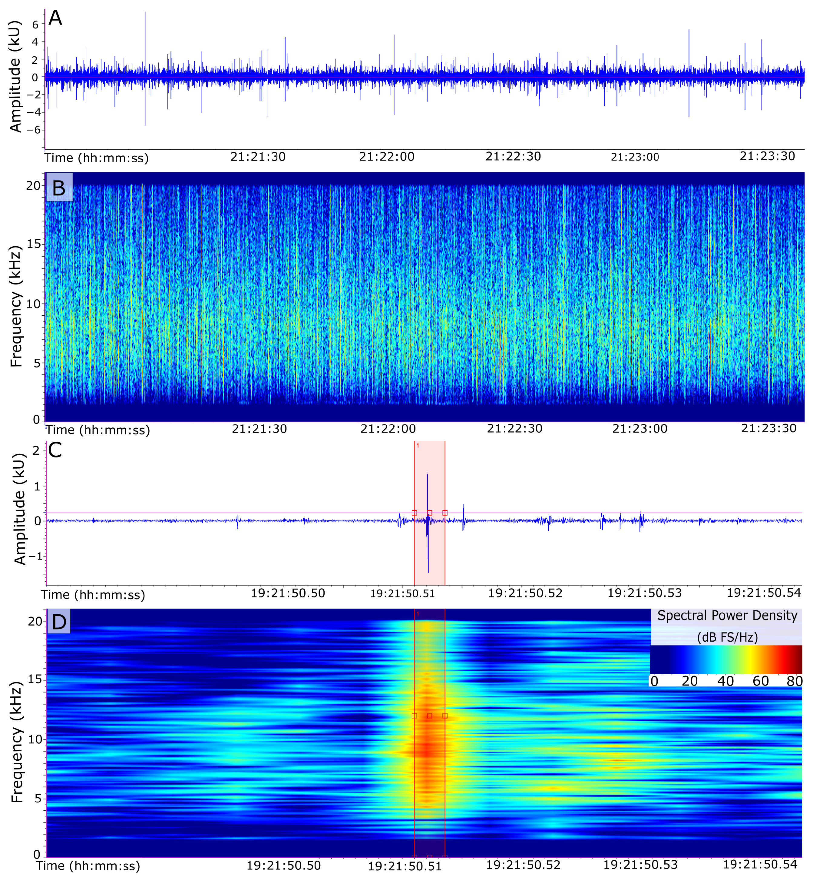
2.3. Measuring Biotic Influence: Snap Rates

Snapping shrimp behavior was quantified using continuous recordings from a SoundTrap 500 hydrophone at SURTASSTN20. Recordings were sampled at 48 kHz then bandpass-filtered (Kaiser window with a default transition bandwidth of 0.02 times the Nyquist frequency, 1.5–20 kHz) to isolate snapping shrimp influence [23], providing a sharp frequency cutoff and preventing any phase distortion. Snap rate was estimated using an amplitude threshold detector in Raven Pro 1.6 (an acoustic analysis software built to discern auditory signals [32]), detecting spikes in waveform intensity in the filtered recordings (Figure 3). An amplitude of 1000 units (1 kU) was chosen as a reasonable intensity threshold to count as a snap, where the dimensionless units are the root-mean-square (RMS) amplitude over the entire selected frequency band, an “effective amplitude” for sound processing [32]. This snap detection algorithm was automated and verified by the random selection of 10 separate 10 s intervals, each of which properly captured only the snaps exceeding the chosen threshold and correctly disregarded quieter snaps. The reported snap rate is the number of snaps that met the intensity threshold in an hour, used as a proxy for the noise created. The snap rate was calculated for data spanning several months in 2020 and 2021, and here is separated into spring (30 January–4 May 2020) and fall/winter (29 September–31 December 2020) deployments for a total of 4515 h analyzed. Measured snap rate variability (noise created) is then compared with calculated noise lost at the surface.

2.4. Calculating Abiotic Influence: Surface Bubble Loss

Wind-driven waves generate whitecaps and turbulence that can create a layer of bubbles at the surface [17,33]. This bubble layer dampens propagation, limits reflection, and increases absorption of sound [15,33]. Wind and wave height data from NDBC Station 41008 were used to calculate noise attenuation through surface bubble loss (SBL) as follows [14]:

$$SBL\left(dB\right)={\displaystyle \frac{1.26\times {10}^{-3}}{sin\theta }}{U}^{1.57}{f}^{0.85},U\ge 6m/s$$

and

$$SBL\left(dB\right)=SBL(U=6m/s)e^{1.2(U-6)},U<6m/s$$

where U is the wind speed, f is the transmission frequency (69 kHz), and $\theta$ is the angle at which the signal meets the surface [14], with a 6 m/s wind speed threshold to account for the difference in sea state once white caps form (Figure 4). The SBL was capped at a maximum of 15 dB to reflect measured limits on sound attenuation as bubbles entrain together and scatter noise at the surface [14,17]. Snapping shrimp are ubiquitous in the densely colonized parts of Gray’s Reef [28], so snapping shrimp are considered sound sources over the entire domain instead of sporadic point sources. Attenuation was calculated with the most conservative reasonable estimate of angle of incidence ($\theta$) at 10° to estimate the higher attenuation loss expected at low incident angles (Figure 4).

2.5. Filtering and Statistical Analysis

A fourth-order low-pass recursive Butterworth filter was used to isolate the low-frequency variability (>40 h). The time series data contained variability on multiple concurrent timescales, and this filter protected trends while removing the higher-frequency components. To reduce autocorrelation, the filtered data were subsampled at a 40 h window for statistical analysis. Data were then normalized by subtracting the mean and dividing by the standard deviation, with significant outliers removed. The Pearson correlation coefficients and associated statistical significance (p-value) were calculated for both the raw and filtered data to quantify the relationship between environmental variables (temperature, wind speed, noise), assuming linear relationships. The ${\mathrm{R}}^2$ value represents the correlation coefficient between the two variables, measuring the variance, and they are paired with p-values lower than 0.01 unless otherwise noted. The Spearman correlation coefficients were chosen for snap rate and detection data to account for non-normality, the sporadic detection patterns, and the discrete nature of hourly count data assuming monotonic (but not necessarily linear) relationships between them and environmental variables. Detection data and snap rates are not expected to be (and are not) normally distributed. Spearman’s rank correlation converts them to a ranking and computes the Pearson correlation on those ranks as a way to measure variability without assuming linearity or normality. Reported ${\mathrm{R}}^2$ values still measured the variance and were paired with p-values lower than 0.01.

3. Results

In this section, we evaluate the relative influence of biotic and abiotic variability in the soundscape by comparing the estimated noise creation by snapping shrimp and the estimated SBL attenuation to measured HF noise levels. Shrimp snapping was compared to predictable environmental variability and these behavior patterns were analyzed as a proxy for noise interference. Wind speed and SBL were compared with shrimp snaps, measured noise, and telemetry detections to isolate the effect of increasing winds and wave height. The balance between noise created and noise lost was tested during high-wind events.

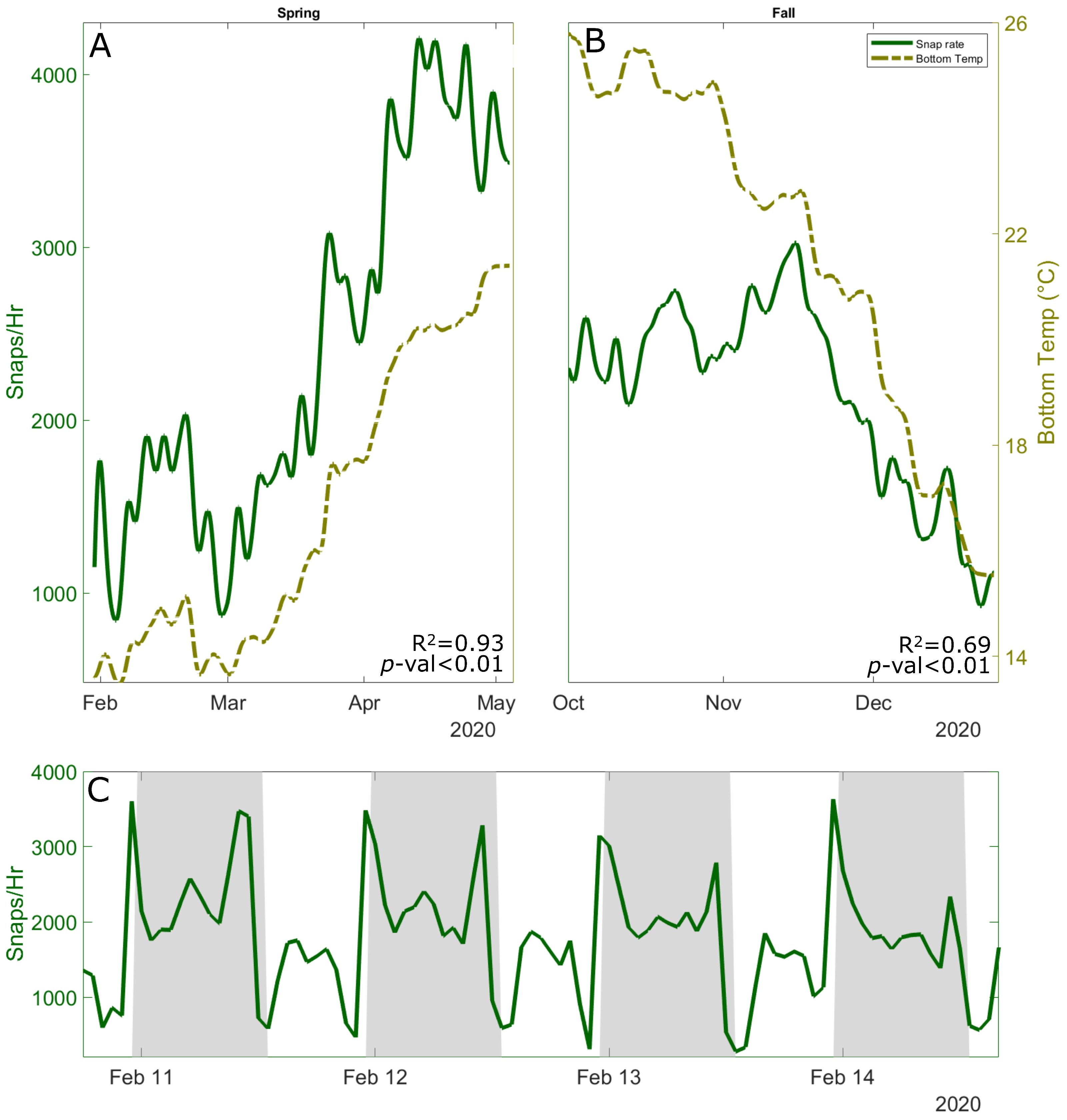
3.1. Variability in Snapping Shrimp Behavior

Bottom temperature appears to be the strongest driver of snapping shrimp behavior (n = 2268 hrs, ${\mathrm{R}}^2$ = 0.93, p-value < 0.01) and resulting HF noise (${\mathrm{R}}^2$ = 0.66, p-value < 0.01), as reflected in observed seasonal trends (Figure 5 and

Table 3. Monthly mean averages for GRNMS. Bottom temperature and noise (50–90 kHz) were collected by transceiver at SURTASSTN20; wind speed (m/s) and SST (°C) were measured by NDBC Station 41008.

Month	Bottom Temp (°C)	Wind Speed (m/s)	Hourly Snaps	HF Noise (mV)	Avg. Detections
February 2020	14.0 ± 0.5	6.45 ± 3.03	1479 ± 736	655 ± 49	2.7 ± 4.2
March 2020	15.4 ± 1.3	4.92 ± 2.57	2012 ± 886	697 ± 45	1.0 ± 1.7
April 2020	19.8 ± 0.9	5.64 ± 2.64	3664 ± 897	746 ± 30	0.4 ± 1.1
May 2020	22.4 ± 0.9	4.97 ± 2.26	3604 ± 1105	760 ± 25	0.3 ± 0.9
October 2020	24.7 ± 0.4	6.12 ± 2.88	2427 ± 767	781 ± 27	0.04 ± 0.3
November 2020	21.8 ± 1.0	6.54 ± 2.77	2503 ± 783	762 ± 30	0.05 ± 0.4
December 2020	17.6 ± 1.2	6.14 ± 3.43	1294 ± 623	697 ± 42	0.40 ± 1.0

). Warming spring temperatures are associated with increased snapping shrimp activity (Figure 5A), while cooling fall waters are associated with decreased snapping activity (Figure 5B). This seasonal increase in background noise interference was inversely related to detection efficiency data; the VR2Tx acoustic telemetry transceiver at SURTASSTN20 detected transmissions from the nearest transceiver (STSNew1) more often in winter, with the average (mean) efficiency dropping lower in summer: February, 13%; March, 9%; April, 4%; May, 3%; June, 3%; July, 4%; August, 0.5%; September, 0.8%; October, 0.8%; November, 0.9%; December, 6% (Table 3).

Diurnal and crepuscular behavior patterns emerged from the data measured at SURTASSTN20 (Figure 5C), with peak shrimp behavior detected at sunset and sunrise followed by low activity levels during the day. When averaged over a canonical day in Figure 6, the highest average number of snaps per hour occurred at sunset (95% confidence interval: 19:00 average, 2960–3459 snaps per hour), followed by sunrise (06:00 average, 2709–3366 snaps per hour). There were relatively high activity levels at sunrise compared with low snap rates mid-day (13:00 average, 1665–2039 snaps per hour) (Figure 6), an average difference of 73% more snaps at sunrise versus midday. Snap rate rose sharply at night and dropped during the day, with a positive (but variable) snap rate increase from day to night, quantified monthly: February 2020, 53.8%; March, 25.1%; April, 13.1%; October, 46.8%; November, 20.2%; December, 59.6% (Figure 5C and Figure 6; Table 3). Snap rate and transmission detection had a statistically significant relationship (p-value < 0.01), and there were far more detections when there were fewer snaps—22.2% more detections at midday when the acoustic environment was more optimal versus sunset when average noise was highest (Figure 6).

There was no observed correlation between wind speed and snap rate (filtered p-value=0.07; raw p-value = 0.53), SBL and snap rate (filtered p-value = 0.04; raw p-value = 0.27), or between significant wave height and snap rate (filtered p-value = 0.37; raw p-value = 0.51).

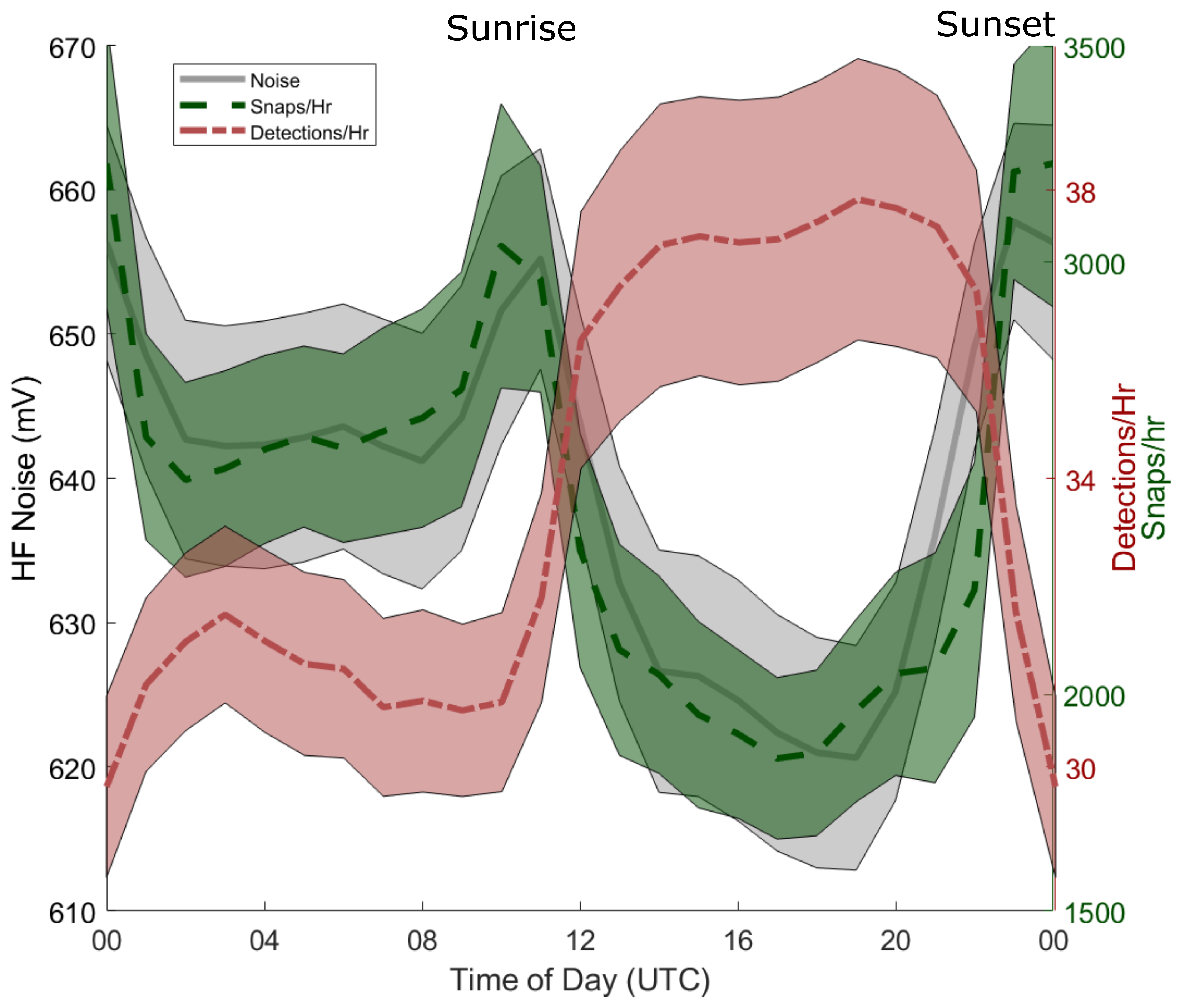
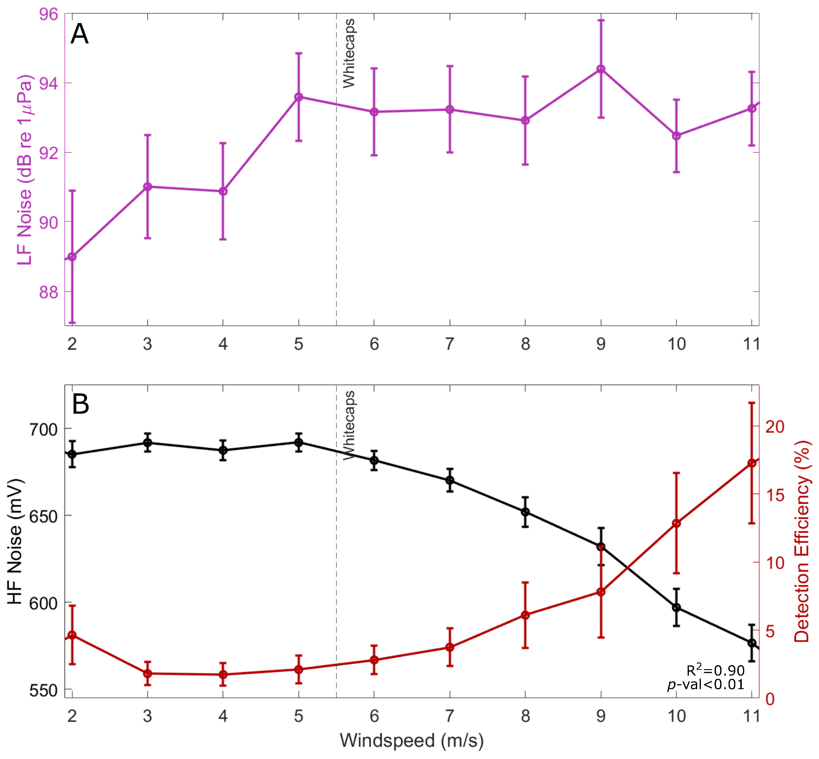
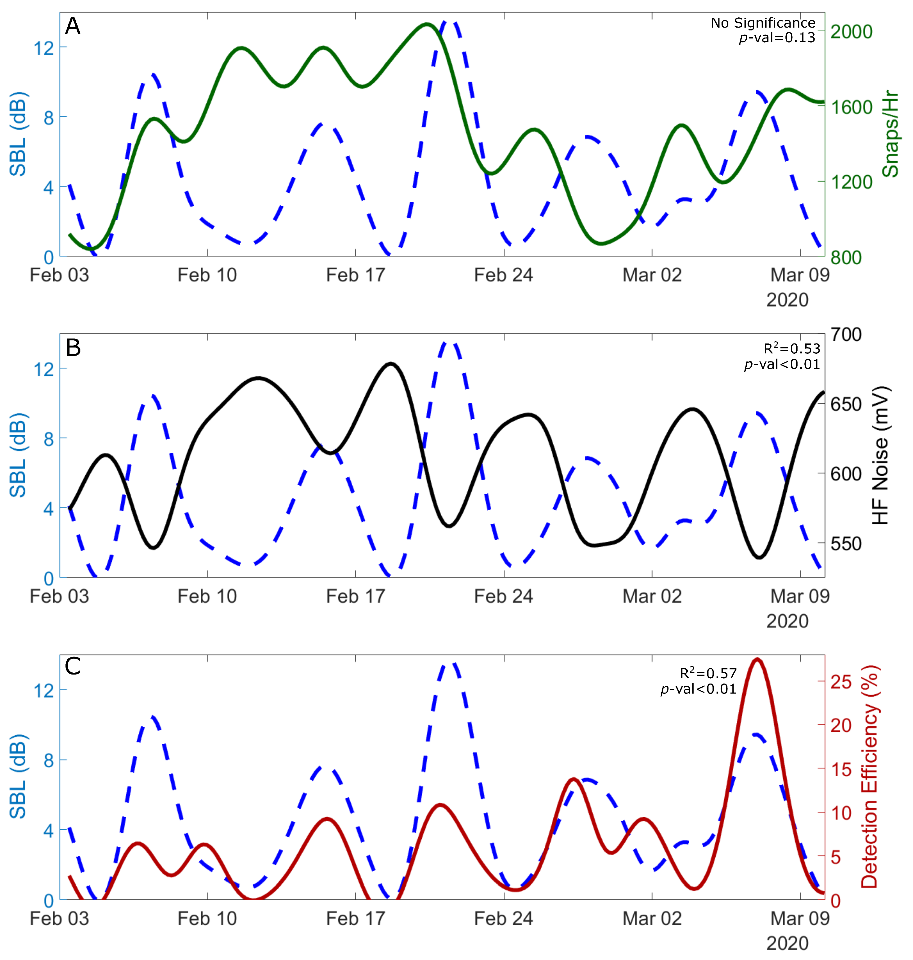
3.2. The Effect of Wind-Driven Attenuation on the Soundscape

During the spring deployment at SURTASSTN20 (2268 h analyzed), wind speeds ranged between 0.2–14.3 m/s (average of 5.7 m/s); calculations of SBL with these values represent the full measured spectrum of SBL attenuation (0–15 dB). The relationship between HF noise and wind speed is statistically significant (${\mathrm{R}}^2$ = 0.30, p-value < 0.01), as is the relationship between HF noise and SBL attenuation (${\mathrm{R}}^2$ = 0.32, p-value < 0.01). Low-frequency (0.17–0.36 kHz) noise increased with wind speed, and stayed relatively constant after whitecaps and the surface bubble layer formed (Figure 7A). In contrast, high-frequency noise (50–90 kHz) dropped quickly with wind speeds greater than 6 m/s; detection efficiency between SURTASSTN20 and STSNew1 rose sharply over this period as potential noise interference dropped (${\mathrm{R}}^2$ = 0.90, p-value < 0.01) (Figure 7B). During specific wind events, the increase in low-frequency noise and decrease in high-frequency noise were both clear, even during nighttime when snapping shrimp were expected to be most active (Figure 8). Snapping shrimp behavior appeared unaffected by increased winds (Figure 9 and Figure 10), suggesting that the same amount of noise is created during periods of high winds but the surface attenuation at the bubble layer lowers HF noise interference (Figure 9).

A stronger pattern between attenuation and noise emerges when isolating high-wind events (average length of 4.5 days): when short-term variability in winds is removed (40 h cutoff), SBL is highly correlated with high-frequency noise (${\mathrm{R}}^2$ = 0.87–0.97, p-values < 0.01) (

Table 4. Isolated wind events ranging from 3.75 to 6.75 days with noise (50–90 kHz) and detections measured at SURTASSTN20. Reported ${\mathrm{R}}^2$ values are paired with p-value < 0.01; lack of value (-) represents no statistical significance (p-value > 0.01).

Dates	Duration (h)	Wind Speed (m/s)	Snap Rate vs. SBL (${\mathrm{R}}^2$)	Noise vs. SBL (${\mathrm{R}}^2$)	Detections vs. SBL (${\mathrm{R}}^2$)
5–10 February	133	1.4–14.2	-	0.89	-
12–18 February	161	0.73–11.0	-	0.97	0.95
30 March–3 April	109	0.8–12.8	-	0.92	0.76
14–18 April	90	2.31–10.8	-	0.91	0.98
28 April–2 May	93	1.3–11.3	0.80	0.91	0.52

; Figure 10 and Figure 11). Figure 10 shows that snapping shrimp activity is responsible for the majority of HF noise creation (Figure 10A) and SBL and HF noise were inversely correlated (Figure 10C) but snapping shrimp activity changed very little with high winds (Figure 10E). After low-pass filtering, wind events appeared as large changes in HF noise (Figure 10D), while snap rates were mostly unaffected (Figure 10B,F). Figure 11 isolates a single wind event to highlight these interactions, showing a strong statistical relationship between SBL and HF noise (Figure 11A,B) and between SBL and detection efficiency (Figure 11C,D), but no correlation between SBL and snapping behavior (Figure 11E,F).

Figure 12 highlights a case study: SBL attenuation is correlated with detection efficiency (p-value < 0.01)—very few (if any) transmissions are detected for days, but efficiency grows to 60–100% when winds are highest. Figure 12A,C include AUV collected density data for added context. High SBL and the resulting decrease in HF noise were closely tied to sporadic spikes in detection efficiency while stratification appeared unrelated, and snapping behavior continued on crepuscular and diurnal patterns regardless of the wind events (Figure 12D; see Supplementary Figures S1 and S2).

4. Discussion

GRNMS is a considered a challenging acoustic environment for telemetry due to the magnitude of measured background noise, and the challenge in interpreting data collected there is further amplified due to large seasonal and diurnal swings in biotic background noise driven by snapping shrimp (Figure 5 and Figure 6), which lead to noisier environments with fewer successful detections (Table 3). The results shown here demonstrate that wind events provide another layer of obfuscation in interpreting the meaning of acoustic telemetry detections, since the interfering noise of snapping shrimp can be attenuated by surface bubble layers generated during high-wind events.

High winds had little to no effect on noise generation by snapping shrimp but resulted in increased high-frequency noise attenuation that appeared to improve acoustic telemetry detection rates. This analysis identifies a mechanism seen in previously observed patterns of increased detections during high-wind events [3]: a loss of high-frequency background noise, reducing interference (Figure 1B; Table 4). Most of the intermediate variability in measured HF noise was explained by the SBL in the form of sound lost at the air–sea interface (Figure 10; Table 4), while snap rate was largely unaffected by wind variability (Figure 11; Table 4).

Quantifying the snap rate with hydrophone data provides the means to determine how much noise was created (versus measured), with large spikes at dusk and dawn as shrimp behavior increases (Figure 5 and Figure 6). Warmer seasonal temperatures were correlated with increased reef activity and more noise created (Figure 5; Table 3). Previous studies that suggest that lower benthic activity may be responsible for the decreased noise levels during high-wind events [26] may have incorrectly attributed measuring less noise to there being less noise created. An experiment showed that impulsive low-frequency sounds (0.05–0.6 kHz) played through an underwater speaker can affect snapping shrimp behavior [34], but the low-frequency noise created by crashing waves ($\tilde{0}$.01–1.5 kHz) did not have the same effect. Our results suggests that noise derived from wind did not affect snap rates. There was no evidence in this study that less biotic noise is created during high winds; more noise was simply lost at the air-sea interface when attenuation was high and reflectance was low.

Calculating surface bubble loss thus appears to be an effective way to estimate noise lost at the air–sea interface and identifies the relationship between the biotic noise being created by snapping shrimp and the abiotic attenuation occurring at high frequencies due to SBL [14,15]. Noise attenuation also occurs coherently as a measure of distance traveled [35]; this loss was not included in our calculations because we did not attempt to perfectly model sound loss but instead offer an effective explanation for the observed variability in the GRNMS soundscape. The significant correlation between measured noise and SBL was strong, especially when isolating events and removing daily and seasonal variability (Figure 11 and Figure 12; Table 4). Wind-driven changes in detection efficiency appeared primarily driven by increased attenuation (Figure 10; Table 4), pointing to the hypothesized abiotic relationship (Figure 1B) being the better explanation of the relationship between winds and detection efficiency at GRNMS. Detection efficiency in the 400–500 m range in a shallow, noisy environment like GRNMS is expected to be low [2,6], so an average of 20% efficiency during high winds (Figure 7) represents reasonable success averaged over January–May when accounting for the expected drops in efficiency due to elevated snapping activity at nighttime (Figure 6) and in warmer waters (Table 3).

In environments where HF background noise is lower and the environment is more optimal for telemetry, SBL may not have such a large effect on telemetry success and wind may even hinder the detection of high-frequency signals. SBL calculations do not consider the proximity of the bubble layer to the instrumentation placement or bottom depth, which may lead to reduced efficiency in shallower environments [19,27,36] where the bubbles may hinder signal pathways or degrade signal strength [37]. Previous research at Gray’s Reef observed that a VR2Tx transceiver in a more protected, sunken part of the reef (FS17) measured far less noise [3]. There was no hydrophone at this location, so we cannot determine if the snap rate for that quieter reef area was different from the analysis above, but high-frequency noise from the telemetry transceiver was much lower than the challenging threshold (650 mV) and detections seemed unaffected by noise [3]. Anecdotally, detection rate decreased with higher winds over some periods in this quieter part of the reef, which may be explained by waves and bubbles hindering reflections at the air–sea interface. There was a significant slope in the bathymetry between FS17 and the closest transmitter (STSNew1, 3.6 m difference), which may have limited the paths that transmissions could take between instruments. Transmissions between these moorings may reflect off the surface between the transmitter and receiver while the surface is calm but attenuate and scatter when winds are high. When background noise is not the limiting factor, a decrease in possible sound pathways between instruments due to reduced surface reflectance may lower detection efficiency [6], and measuring the depth of the surface bubble layer [18] may explain reduced detection efficiency.

In situ range testing may not accurately represent the effective distance of the technology if it does not correctly characterize the entire range of likely environmental conditions; users may be aware of the importance of testing transmitter and receiver pairings in their specific environment but may not fully account for temporal variability [1]. The findings presented here point to a novel relationship that, if understood, can be leveraged: wind events may attenuate interference from biotic background noise from snapping shrimp, thereby increasing the effectiveness of the telemetry in challenging acoustic environments. Snapping shrimp are found at a wide range of latitudes [23] and can affect acoustic telemetry; local sources of noise and attenuation need to be included as context when analyzing acoustic data collected in these environments. When measuring the amount of general high-frequency noise, users should consider whether noise interference is going to be important and what processes may help or hinder transmission detection.

Transmission power and frequency are delicate balances in complex marine environments. Transmissions with higher power can be reliably detected from farther away, but risk interfering with themselves and drain battery at a higher rate [38]. Tagging fish takes time and resources, and lower-power transmissions mean the tag will be effective for longer. Selecting the transmission frequency also contains trade-offs. If a transmission is closer to the 20 kHz limit, it attenuates slower but increases the sources of noise interference; if you increase transmission frequency (>100 kHz), there may be lower background noise interference but the signal attenuates quicker and will not travel as far. More experimentation should be carried out on how to best account for high-noise environments.

Further Work

The acoustic telemetry community is attempting to meet the challenge of background noise by developing sensors that better account for higher noise levels by increasing the filtering performed by the receivers, but the “high-noise” environments in which these instruments have been tested have significantly less noise than the study site given here. For example, the Innovasea NexTrak R1 was tested in a 2024 technical report focused around testing in a “high-noise environment” that appeared to exceed the 650 mV challenging threshold only a small percentage of the time [39], whereas parts of GRNMS have average noise levels that exceed that threshold for almost the entirety of summer (>95% of h) (Table 3). More work needs to be carried out on this type of environment to determine whether the noise levels are as detrimental (or in worst cases, prohibitive) when using newer technologies. Instrumentation with signal strength metrics, measuring not only if a detection occurred but the intensity of the signal, would help estimate transmission loss in these high-noise environments and explain measured changes in effective detection range.

Next steps to define the effect of surface and bottom boundary layers on signal transmissions should include modeling the signal propagation under different environmental conditions, connecting the decrease in background noise with the modeled bubble plume depth and resulting limited reflectance/pathways between tags and receivers. Wind does not have a uniform effect on efficiency, and more targeted experiments can help define why.

References

1. Payne, N.L.; Gillanders, B.M.; Webber, D.M.; Semmens, J.M. Interpreting diel activity patterns from acoustic telemetry: The need for controls. Mar. Ecol. Prog. Ser. 2010, 419, 295–301. [Google Scholar] [CrossRef]
2. Edwards, C.R.; Cho, S.; Zhang, F.; Fangman, S. Field and Numerical Studies to Assess Performance of Acoustic Telemetry Collected by Autonomous Mobile Platforms, 2014. In Review of Scientific Research in and around the Designated Research Area of Gray’s Reef National Marine Sanctuary; National Marine Sanctuaries Conservation Series ONMS-20-08; U.S. Department of Commerce, National Oceanic and Atmospheric Administration, Office of National Marine Sanctuaries: Silver Spring, MD, USA, 2020; pp. 157–177. [Google Scholar]
3. McQuarrie, F.; Woodson, C.B.; Edwards, C.R. Analyzing Tidal, Diurnal, Synoptic, and Seasonal Drivers of Acoustic Telemetry Efficiency on a Coastal Reef. In Proceedings of the Marine Technology Society Soc’s 2023 OCEANS Conference 2023, Biloxi, MS, USA, 25–28 September 2023. [Google Scholar] [CrossRef]
4. Cho, S.; Zhang, F.; Edwards, C. Tidal variability of acoustic detection. In Proceedings of the 2016 IEEE International Conferences on Big Data and Cloud Computing (BDCloud), Social Computing and Networking (SocialCom), Sustainable Computing and Communications (SustainCom) (BDCloud-SocialCom-SustainCom), Atlanta, GA, USA, 8–10 October 2016; pp. 431–436. [Google Scholar] [CrossRef]
5. Gjelland, K.; Hedger, R. Environmental influence on transmitter detection probability in biotelemetry: Developing a general model of acoustic transmission. Methods Ecol. Evol. 2013, 4, 665–674. [Google Scholar] [CrossRef]
6. McQuarrie, F.; Woodson, C.B.; Edwards, C. Modeling Acoustic Telemetry Detection Ranges in a Shallow Coastal Environment. In Proceedings of the 15th International Conference on Underwater Networks & Systems, Guangdong, China, 22–24 November 2021. [Google Scholar] [CrossRef]
7. Oliver, M.; Breece, M.; Haulsee, D.; Cimino, M.; Kohut, J.; Aragon, D.; Fox, D. Factors affecting detection efficiency of mobile telemetry. Anim. Biotelemetry 2017, 5, 1–9. [Google Scholar] [CrossRef]
8. Huveneers, C.; Simpfendorfer, C.; Kim, S.; Semmens, J.; Hobday, A.; Pederson, H.; Stieglitz, T.; Vallee, R.; Webber, D.; Heupel, M.; et al. The influence of environmental parameters on the performance and detection range of acoustic receivers. Methods Ecol. Evol. 2016, 7, 825–835. [Google Scholar] [CrossRef]
9. Kendall, M.S.; Williams, B.L.; Ellis, R.D.; Flaherty-Walia, K.E.; Collins, A.B.; Roberson, K.W. Measuring and understanding receiver efficiency in your acoustic telemetry array. Fish. Res. 2021, 234, 105802. [Google Scholar] [CrossRef]
10. Ellis, R.D.; Flaherty-Walia, K.E.; Collins, A.B.; Bickford, J.W.; Boucek, R.; Burnsed, S.L.W.; Lowerre-Barbieri, S.K. Acoustic telemetry array evolution: From species- and project-specific designs to large-scale, multispecies, cooperative networks. Fish. Res. 2019, 209, 186–195. [Google Scholar] [CrossRef]
11. Blanton, J.; Werner, F.; Kim, C.; Atkinson, L.; Lee, T.; Savidge, D. Transport and fate of low-density water in a coastal frontal zone. Cont. Shelf Res. 1994, 14, 401–427. [Google Scholar] [CrossRef]
12. Mackenzie, K. Nine-term equation for sound speed in the oceans. J. Acoust. Soc. Am. 1981, 70, 807–812. [Google Scholar] [CrossRef]
13. Stojanovic, M.; Preisig, J. Underwater Acoustic Communication Channels: Propagation Models and Statistical Characterization. IEEE Commun. Mag. 2009, 47, 84–89. [Google Scholar] [CrossRef]
14. UWAPL. High-Frequency Ocean Environmental Acoustic Models Handbook; Technical Report; Applied Physics Laboratory University of Washington: Seattle, WA, USA, 1994. [Google Scholar]
15. Hildebrand, J.; Frasier, K.; Baumann-Pickering, S.; Wiggins, S. An Empirical model for wind-generated ocean noise. J. Acoust. Soc. Am. 2021, 149, 4516–4533. [Google Scholar] [CrossRef]
16. Huang, C.; Yeh, C.; Liu, K. Bubble entrainment and underwater noise caused by a single water drop falling on the surface of freshwater and saltwater. Phys. Fluids 2024, 36, 022109. [Google Scholar] [CrossRef]
17. Prosperetti, A. Bubble-related ambient noise in the ocean. J. Acoust. Soc. Am. 1988, 84, 1042–1054. [Google Scholar] [CrossRef]
18. Pelaez-Zapata, D.; Pakrashi, V.; Dias, F. Dynamics of bubble plumes produced by breaking waves. J. Phys. Oceanogr. 2024, 54, 2059–2071. [Google Scholar] [CrossRef]
19. Swadling, D.S.; Knott, N.A.; Rees, M.J.; Pederson, H.; Adams, K.R.; Taylor, M.D.; Davis, A.R. Seagrass canopies and the performance of acoustic telemetry: Implications for the interpretation of fish movements. Anim. Biotelemetry 2020, 8, 1–13. [Google Scholar] [CrossRef]
20. Delory, E.; Toma, D.M.; Rio, J.D.; Molina, P.R.; Toma, D.; Rio, J.D.; Ruiz, P.; Corradino, L.; Brault, P.; Fiquet, F. Nexos Objectives in Multi-Platform Underwater Passive Acoustics. In Proceedings of the 2nd International Conference and Exhibition on Underwater Acoustics, Rhodes, Greece, 22–27 June 2014. [Google Scholar]
21. Stanley, J.; Parijs, S.V.; Davis, G.; Sullivan, M.; Hatch, L. Monitoring spatial and temporal soundscape features within ecologically significant U.S. National Marine Sanctuaries. Ecol. Appl. 2021, 31, e02439. [Google Scholar] [CrossRef]
22. Pincock, D.G. Understanding the Performance of VEMCO 69 kHz Single Frequency Acoustic Telemetry; Technical Report; Amirix: Halifax, NS, Canada, 2008. [Google Scholar]
23. Bohnenstiehl, D.R.; Lillis, A.; Eggleston, D.B. The curious acoustic behavior of estuarine snapping shrimp: Temporal patterns of snapping shrimp sound in sub-tidal oyster reef habitat. PLoS ONE 2016, 11, 3691. [Google Scholar] [CrossRef]
24. Song, Z.; Ou, W.; Su, Y.; Li, H.; Fan, W.; Sun, S.; Wang, T.; Xu, X.; Zhang, Y. Sounds of snapping shrimp (Alpheidae) as important input to the soundscape in the southeast China coastal sea. Front. Mar. Sci. 2023, 10, 9003. [Google Scholar] [CrossRef]
25. VEMCO. Receiver Noise Measurements; Technical Report; Innovasea-VEMCO: Boston, MA, USA, 2021. [Google Scholar]
26. Jung, S.K.; Choi, B.K.; Kim, B.C.; Kim, B.N.; Kim, S.H.; Park, Y.; Lee, Y.K. Seawater temperature and wind speed dependences and diurnal variation of ambient noise at the snapping shrimp colony in shallow water of southern sea of Korea. Jpn. J. Appl. Phys. 2012, 51, 07GG09. [Google Scholar] [CrossRef]
27. Edwards, J.E.; Buijse, H.V.W.; Bijleveld, A.I. Gone with the wind: Environmental variation influences detection efficiency in a coastal acoustic telemetry array. Anim. Biotelemetry 2024, 12, 21. [Google Scholar] [CrossRef]
28. ONMS. Gray’s Reef Condition Report 2012 Addendum: Gray’s Reef; NOAA Condition Report; National Oceanic and Atmospheric Administration: Silver Spring, MD, USA, 2012. [Google Scholar]
29. Blanton, J.; Atkinson, L.P. Transport and fate of river discharge on the continental shelf of the southeastern United States. J. Geophys. Res. Oceans 1983, 88, 4730–4738. [Google Scholar] [CrossRef]
30. Scherrer, S.; Rideout, B.; Giorli, G.; Nosal, E.; Weng, K. Depth-and range-dependent variation in the perfomance of aquatic telemetry systems: Understanding and predicting the susceptibility of acoustic tag-receiver pairs to close proximity detection interference. PeerJ 2018, 6, e4249. [Google Scholar] [CrossRef] [PubMed]
31. Binder, T.; Holbrook, C.; Hayden, T.; Krueger, C. Spatial and temporal variation in positioning probability of acoustic telemetry arrays: Fine-scale variability and complex interactions. Anim. Biotelemetry 2016, 4, 1–15. [Google Scholar] [CrossRef]
32. K. Lisa Yang Center for Conservation Bioacoustics. Raven Pro: Interactive Sound Analysis Software (Version 1.6.5). 2024. Available online: https://www.ravensoundsoftware.com/software/raven-pro/ (accessed on 14 August 2024).
33. Ocean Acoustics Toolbox, Office of Naval Research, USA, Published 1999/Updated 3/2023. Available online: http://oalib.hlsresearch.com/AcousticsToolbox/ (accessed on 30 April 2024).
34. Spiga, I. The acoustic response of snapping shrimp to synthetic impulsive acoustic stimuli between 50 and 600 Hz. Mar. Pollut. Bull. 2022, 185, 4238. [Google Scholar] [CrossRef]
35. Huang, J.; Barbeau, M.; Blouin, S.; Hamm, C.; Taillefer, M. Simulation and modeling of hydro acoustic communication channels with wide band attenuation and ambient noise. Int. J. Parallel Emergent Distrib. Syst. 2017, 32, 466–485. [Google Scholar] [CrossRef]
36. Reubens, J.; Verhelst, P.; van der Knaap, I.; Deneudt, K.; Moens, T.; Hernandez, F. Environmental factors influence the detection probability in acoustic telemetry in a marine environment: Results from a new setup. Hydrobiologia 2019, 845, 81–94. [Google Scholar] [CrossRef]
37. Chua, G.; Chitre, M.; Deane, G. Impact of Persistent Bubbles on Underwater Acoustic Communication. In Proceedings of the 2018 Fourth Underwater Communications and Networking Conference (UComms), Lerici, Italy, 28–30 August 2018. [Google Scholar]
38. Kessel, S.T.; Hussey, N.E.; Webber, D.M.; Gruber, S.H.; Young, J.M.; Smale, M.J.; Fisk, A.T. Close proximity detection interference with acoustic telemetry: The importance of considering tag power output in low ambient noise environments. Anim. Biotelemetry 2015, 3, 1–14. [Google Scholar] [CrossRef]
39. Pederson, H.; Bowen, E.; McDonald, J.; Smedbol, S.; Jaine, F. Field Testing the New NexTrak R1 Acoustic Receiver in a High Noise Environment; Technical Report; Innovasea: Boston, MA, USA, 2024. [Google Scholar]
Figure 1. Schematic detailing the hypothesized relationships between wind and detection efficiency. (A) The biotic hypothesis: As winds increase, snapping shrimp are less active. leading to less noise being created and higher detection efficiency of transmissions. (B) The abiotic hypothesis: As winds increase, snapping shrimp are unaffected and create the same amount of noise, but there is significant sound attenuation due to surface bubble loss (SBL). Illustration by Lee Ann DeLeo (SkIO/UGA).
Jmse 13 00517 g001
Figure 2. Habitat characterization for SURTASSTN20 at GRNMS. Colors denote bottom composition. Map credit: Alison Soss (NOAA/GRNMS).
Jmse 13 00517 g002
Figure 3. SoundTrap 500 recordings were bandpass-filtered (1.5–20 kHz), visualized in Raven Pro as (A) full-spectrum waveform with RMS amplitude (blue) and (B) spectrogram, plotting intensity (dB FS/Hz) normalized to 1 Hz bandwidth. (C) Example waveform amplitude (blue line) identifying single snap exceeding 1000 U threshold (shaded in red); (D) spectrogram from same time (snap shaded in red).
Jmse 13 00517 g003
Figure 4. Surface Bubble Loss (SBL) calculated at 69 kHz, the transmission frequency and center of the HF noise measurement (50–90 kHz). A range of angles from 2 to 90° are plotted with 10° bolded to highlight the angle chosen for this analysis. Lower angles and higher frequencies increase SBL attenuation.
Jmse 13 00517 g004
Figure 5. Temporal variability at SURTASSTN20. (A) Low-pass-filtered bottom temperature (light green, dashed) and snapping shrimp snap rate (dark green, solid) in (A) spring and (B) fall. (C) Snap rate (green) is plotted with night time shaded to highlight crepuscular and diurnal behavior patterns. Times in UTC.
Jmse 13 00517 g005
Figure 6. Canonical day averages: HF noise (gray), shrimp snap rate (green), and hourly detections (red). HF noise and transmission detections are from SURTASS05IN.
Jmse 13 00517 g006
Figure 7. Binned averaging from the Spring deployment at SURTASSTN20. (A) Low-frequency (0.17–0.36 kHz) noise measured by SoundTrap 500 hydrophone; (B) high-frequency (50–90 kHz) noise measured by VR2Tx transceiver, and detection efficiency between SURTASSTN20 and STSNew1. The formation of whitecaps is noted vertically (–).
Jmse 13 00517 g007
Figure 8. Comparison between (A,B) calm and (C,D) high-wind scenarios. Low-frequency (0.17–0.36 kHz) noise was measured by SoundTrap 500 hydrophone; high-frequency (50–90 kHz) noise was measured by VR2Tx transceiver. Nighttime is shaded.
Jmse 13 00517 g008
Figure 9. Data from SURTASSTN20 in Spring 2020. Calculated SBL (blue dashed) versus (A) snapping shrimp activity (green), (B) HF noise (black), and (C) detection efficiency (red) between SURTASSTN20 and STSNew1, 440 m away.
Jmse 13 00517 g009
Figure 10. Hourly averages from spring (n = 2268 h) of (A) raw and (B) filtered snap rate and HF noise (mV), on log scale; (C) raw and (D) filtered SBL (dB) and HF noise (mV); (E) raw and (F) filtered snap rate and wind speed (m/s). Marker color represents date range, January (blue) to May (yellow). Reported statistics include all plotted data; “no significance” represents p-values > 0.01. Binned averages are shown over raw data (black markers) in (A,C,E), and significant wind events are denoted (black lines) in (B,D,F). See Figure 11 for closer examination of isolated wind event (*).
Jmse 13 00517 g010
Figure 11. Example of a single wind event, 19–25 February 2020, with 0.3–14.3 m/s wind speed. (A) Raw and (B) low-pass SBL (dB) and HF noise (mV), (C) raw and (D) low-pass SBL (dB) and detections, and (E) raw and (F) low-pass SBL (dB) and snap rate.
Jmse 13 00517 g011
Figure 12. Data from SURTASSTN20, 22 April to 4 May 2020. (A) Glider data measuring the water column’s bulk density stratification (color); (B) HF noise (black) plotted against hourly detections (red) between SURTASSTN20 and STSNew1, with “challenging environment” (650 mV) denoted (–); (C) calculated SBL (blue) and AUV-measured density stratification (black); (D) snap rate binned hourly (green). All times in UTC.
Jmse 13 00517 g012