Physics-Guided Self-Supervised Learning Full Waveform Inversion with Pretraining on Simultaneous Source

Abstract

Full waveform inversion (FWI) is an established precise velocity estimation tool for seismic exploration. Machine learning-based FWI could plausibly circumvent the long-standing cycle-skipping problem of traditional model-driven methods. The physics-guided self-supervised FWI is appealing in that it avoids having to make tedious efforts in terms of label generation for supervised methods. One way is to employ an inversion network to convert the seismic shot gathers into a velocity model. The objective function is to minimize the difference between the recorded seismic data and the synthetic data by solving the wave equation using the inverted velocity model. To further improve the efficiency, we propose a two-stage training strategy for the self-supervised learning FWI. The first stage is to pretrain the inversion network using a simultaneous source for a large-scale velocity model with high efficiency. The second stage is switched to modeling the separate shot gathers for an accurate measurement of the seismic data to invert the velocity model details. The inversion network is a partial convolution attention modified UNet (PCAMUNet), which combines local feature extraction with global information integration to achieve high-resolution velocity model estimation from seismic shot gathers. The time-domain 2D acoustic wave equation serves as the physical constraint in this self-supervised framework. Different loss functions are used for the two stages, that is, the waveform loss with time weighting for the first stage (simultaneous source) and the hybrid waveform with time weighting and logarithmic envelope loss for the second stage (separate source). Comparative experiments demonstrate that the proposed approach improves both inversion accuracy and efficiency on the Marmousi2 model, Overthrust model, and BP model tests. Moreover, the method exhibits excellent noise resistance and stability when low-frequency data component is missing.

1. Introduction

Precise underground velocity models are crucial for accurate subsurface imaging, stratigraphical interpretation, and reservoir characterization in seismic exploration. Full waveform inversion (FWI) [1] harnesses the kinematic and dynamic information of the wavefield and can theoretically construct a high-resolution velocity model. FWI iteratively refines the velocity model through the minimization of discrepancies between observed and synthetic seismic data. Despite the potential advantage, FWI faces significant challenges posed by various limitations, such as the lack of low-frequency component in seismic data, noise interference, and restricted observation systems. These constraints lead to issues such as the propensity of converging to local minima and the high computational cost.

In recent years, the rapid development of deep learning (DL) [2] technology has been widely applied in seismic exploration [3]. DL methods excel in their powerful nonlinear mapping capabilities, offering alternative solutions for tackling the velocity inversion problems, as demonstrated by pioneering works applying machine learning to FWI [4,5,6]. Drawing upon the power of big data training, Yang et al. [7] introduced a supervised data-driven velocity inversion method, achieving nonlinear mapping from the multi-shot seismic data to the corresponding velocity model. Wu et al. [8] designed InversionNet based on an encoder–decoder architecture, which demonstrated a superior performance compared to traditional FWI under simple geological conditions. Zhang et al. [9] developed VelocityGAN, leveraging generative adversarial networks (GANs) to enhance the accuracy of velocity model generation. Li et al. [10] developed a hybrid network to estimate the velocity model from shot gathers. It effectively reduces the sensitivity of inversion to the initial model. Li et al. [11] designed a multi-branch attention UNet network (MAU-Net) for velocity inversion, where the data branch extracts features from the data domain and the model branch integrates low-frequency model information, effectively reducing the dependency of inversion on the initial model. Additionally, researchers have conducted extensive exploration on data-driven FWI methods [12,13,14]. While data-driven DL-based FWI methods avoid the cycle skipping and alleviate the computation cost and dependency on the initial model, supervised learning framework demands vast amounts of labeled data and often lack generalization to data and models with different distributions.

To address the aforementioned challenges, researchers are gradually shifting towards the model and data dual-driven inversion framework. The dual-driven framework simultaneously integrates physical guidance into the network training process, thereby enhancing the interpretability of inversion results, while also retaining the merits of the data-driven framework. Physics-guided DL can be integrated with various components, such as envelope information [15], domain-independent self-supervised learning [16], continuous and implicit representations [17], the competitive learning of generative adversarial network [18], and physics-based physics-informed neural network (PINN) [19]. Dhara and Sen [20] presented a DL-based FWI technique that integrates encoder–decoder network with physical forward modeling. This approach generates synthetic seismic data using a wave equation and minimizes the difference between observed and synthetic data, eliminating the need for the initial model and labeled data. Jin et al. [21] and Liu et al. [22] followed a similar framework. To accelerate the convergence of the network, Muller et al. [23] utilized supervised pre-training strategy with a simple layered velocity model dataset and applied transfer learning on target dataset inversion. Similarly, transfer learning has been shown to effectively boost the robustness and convergence of training PINN for high-frequency and multi-scale problems by starting with simple smooth models and fine-tuning for more complex scenarios [24]. However, the improvement in accuracy and convergence depends on the similarity between pretraining and target velocity models.

Additionally, a suitable loss function is significant to reduce cycle skipping and avoid local minima for FWI. While waveform misfit functions are common for FWI methods, various loss functions have been explored to make a balance between stability and accuracy. Shin and Cha [25] introduced a waveform inversion algorithm using the logarithmic wavefield objective function in the Laplace domain. Alkhalifah and Song [26] employed a modified source function in the wave equation for wavefield inversion. Bozdağ et al. [27] proposed a novel FWI misfit function leveraging discrepancies in an instantaneous phase and enveloped between observed and synthetic seismograms. Du et al. [28] considered a multi-objective loss function, combining the mean square error (MSE), multiscale structure similarity (MS-SSIM), and the binary cross entropy (BCE) losses for optimization. Sun et al. [29] proposed learning a robust misfit function based on machine learning for FWI. Saad et al. [30] employed a Siamese network to transform simulated and observed seismic data into a shared latent space for robust discrepancy computation.

In this paper, we propose a two-stage training strategy for the physics-guided self-supervised FWI to further improve efficiency. The first stage implements the simultaneous source to generate a super-shot gather for the fast iteration inversion of smooth background velocity. The second stage utilizes the separate shot gathers for high accurate inversion. The physics-guided inversion framework consists of the partial convolution attention modified UNet (PCAMUNet) and a forward operator derived from the finite difference approximation of time domain 2D acoustic wave equation. The approach utilizes different loss functions for the two stages, that is, waveform loss with time weighting for the first stage, and a combination of the waveform with time weighting and logarithmic envelope loss for the second stage.

The subsequent sections of this paper are structured in the following manner. In Section 2, the proposed method is described in detail. In Section 3, comprehensive experimental comparison results on Marmousi2 model, Overthrust model, and the BP model are presented to validate the inversion performance of the proposed method. Section 4 further discusses how noise and missing low-frequency components in observed seismic data affect the inversion performance of the proposed method. Section 5 offers a summary of the paper.

2. Methodology

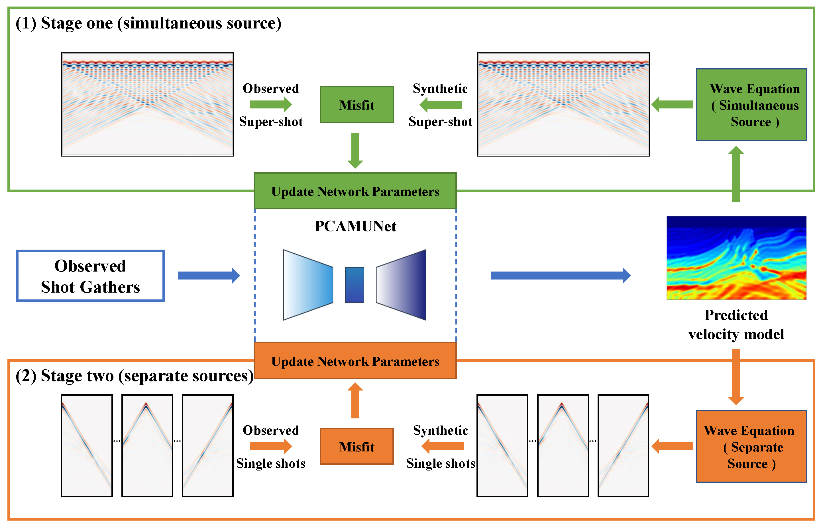
2.1. Physics-Guided Self-Supervised Inversion Framework

As depicted in Figure 1, the training of the proposed method includes feeding the inversion network shot gathers and predicting the velocity model. Subsequently, the corresponding synthetic data is generated by feeding the velocity model into the wave equation. The automatic differentiation-based backpropagation process leverages the gradient of the misfit between the synthetic and observed seismic data to update the network parameters, thereby achieving a reparameterized representation of the subsurface medium parameters. The proposed two-stage training strategy (the first stage: simultaneous source, the second stage: separate source) devises the forward simulations with different sources for loss function calculation.

The physics-guided self-supervised inversion framework eliminates the requirement for velocity labels, thus overcoming the limitations of supervised learning. The inversion process, performed without requiring an initial model, follows the low-frequency bias principle [31] and automatically inverts the velocity model from low to high wavenumbers [32]. By fully leveraging the constraints of the physical equation, the framework ensures that the inversion results align with the physical principles of seismic wave propagation, enhancing the physical interpretability of the results. Unlike conventional model-based inversion, the self-supervised framework utilizes neural network parameterization to implicitly induce regularization effects. In contrast to purely data-driven methodologies, the integration of physics-driven guidance in the dual-driven framework promotes stability on the inversion outcomes.

2.2. Inversion Network Architecture

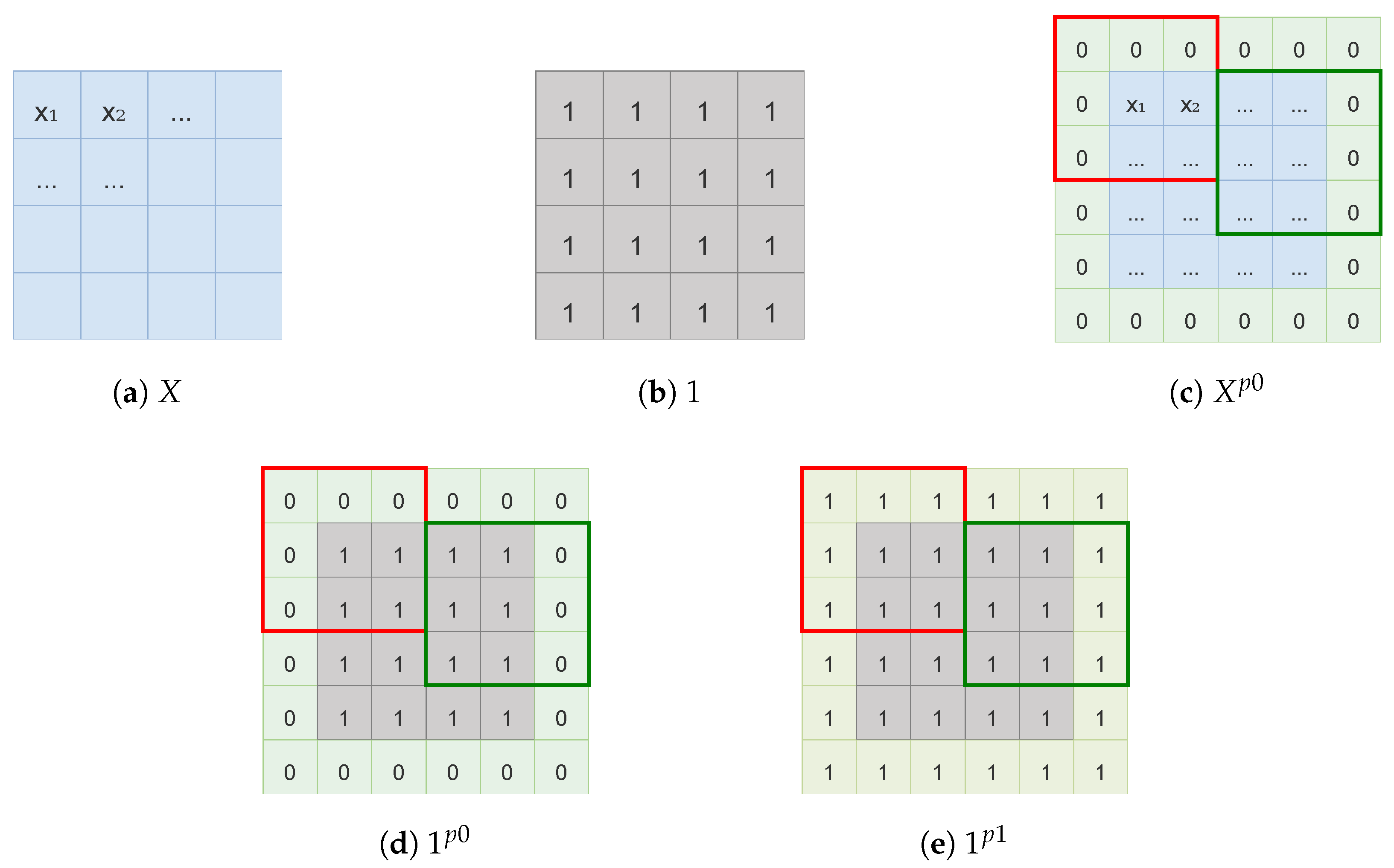
2.2.1. The Partial Convolution Component

When processing bounded data, standard convolution operations typically employ zero-padding to maintain feature map dimensions, which may introduce boundary artifacts and compromise feature extraction accuracy. To address this limitation, partial convolution (PConv) [33] was proposed, incorporating a dynamic weight recalibration mechanism that distinguishes between valid and padded regions through adaptive weighting:

$$y_{(i,j)}=W^T{X}_{(i,j)}^{p0}·r_{(i,j)}+b,$$

(1)

$$r_{(i,j)}={\displaystyle \frac{\left|\right|1_{(i,j)}^{p1}{\left|\right|}_1}{\left|\right|1_{(i,j)}^{p0}{\left|\right|}_1}},$$

(2)

where W is the filter weight matrix; $r_{(i,j)}$ represents the scaling factor for valid regions in the convolutional window; $X_{(i,j)}^{p0}$ denotes the zero padded result of the input feature $X_{(i,j)}$; $1_{(i,j)}^{p1}$ and $1_{(i,j)}^{p0}$ denote the one padded and zero padded result of $1_{(i,j)}$, respectively. The visualization of the examples can be found in Figure 2. PConv dynamically adjusts convolutional weights by explicitly distinguishing valid data regions from padded areas, demonstrating robustness and adaptability.

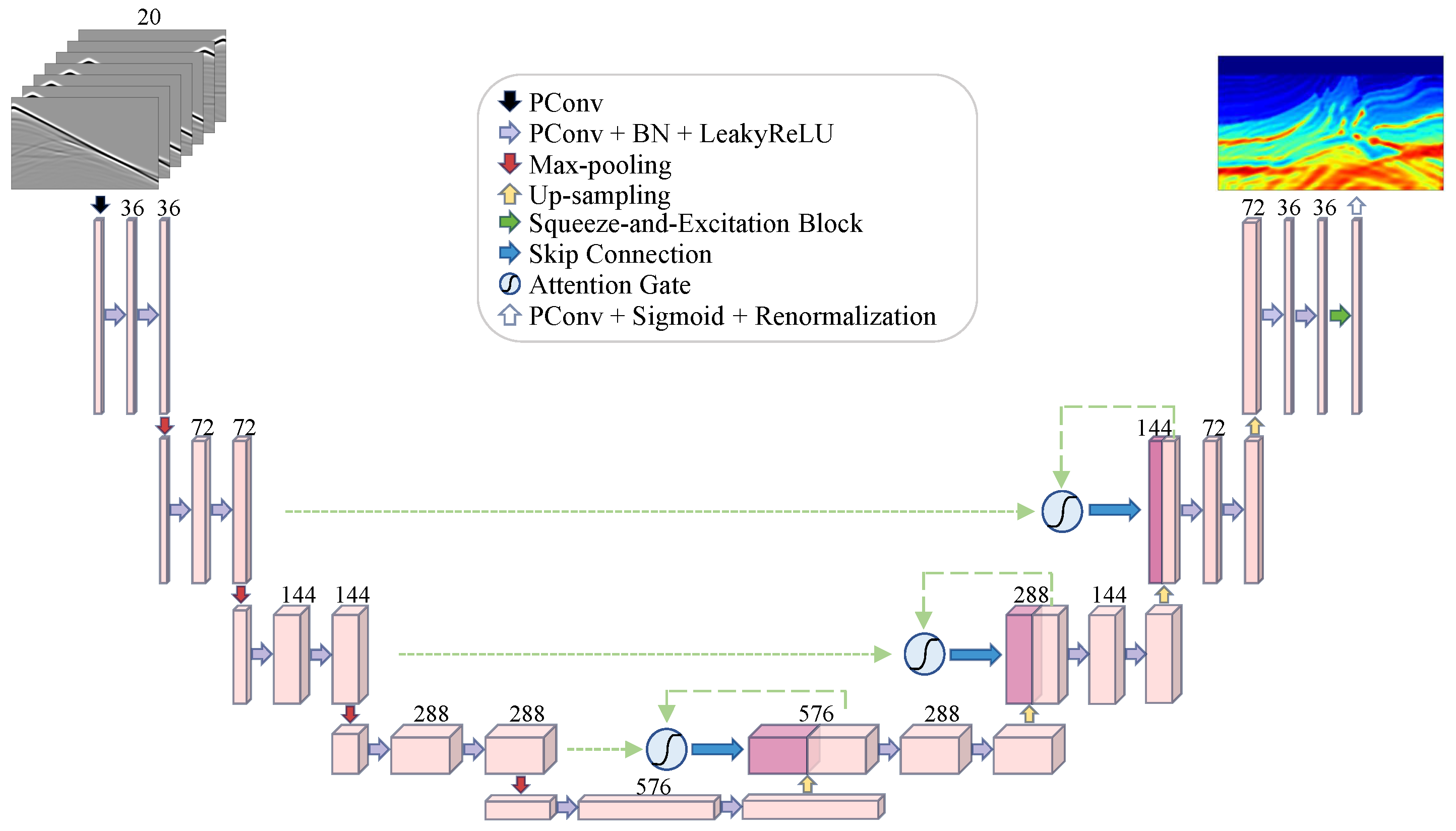
2.2.2. The PConv Attention Modified UNet (PCAMUNet) Architecture

By integrating the Modified UNet (MUNet) [23] with an Attention Gate (AG) mechanism [34], the Squeeze-and-Excitation (SE) block [35] and PConv, a PConv attention modified UNet (PCAMUNet) is devised for FWI. As illustrated in Figure 3, PCAMUNet is tasked with converting time-domain shot gathers into a depth-domain velocity model. To reconcile the dimension mismatch between the input and output in the UNet, the down-sampling operator is essential. After conducting an ablation experiment among various down-sampling operators, including uniform down-sampling, the sampling matrix [28], the LocallyConnected2d operator, the standard convolution (Conv) operator, and PConv operator, we opted for the PConv down-sampling operator.

The PCAMUNet, following the PConv down-sampling operator, is structured into two primary components: an encoder dedicated to feature extraction and a decoder tasked with velocity model feature reconstruction. The encoder includes 4 down-sampling modules, each equipped with 2 PConv blocks and a 2 × 2 max-pooling layer, doubling the feature channels while halving the spatial dimensions. Conversely, the decoder fuses low-resolution maps with encoded spatial information to produce high-resolution feature maps. After each up-sampling module, the channel number halves while feature map size doubles. The first three up-sampling modules each consist of a 2 × 2 up-sampling layer, 2 PConv blocks, and a skip connection, whereas the final up-sampling module excludes the skip connection to avoid source footprint artifacts. Prior to the skip connection, AG mechanisms learn weight coefficients to modulate the down-sampled feature maps, highlighting important areas and suppressing trivial regions. Therefore, this process ensures that concatenated features retain essential spatial information, enhancing the learning capabilities of the PCAMUNet. Following the final up-sampling module, the SE channel attention block dynamically adjusts feature channels, making the features focus on the most important information. This improvement is inspired by the observation that the channel feature maps produced by the final up-sampling module focus on distinct regions of the output velocity model. In the last layer, a Sigmoid function is employed to normalize the feature values, followed by a denormalization step that adjusts the value range of the velocity model. Each PConv block comprises a 3 × 3 PConv operator, a batch normalization (BN) layer, and Leaky ReLU activation function. The numbers atop the cube in Figure 3 are the quantity of feature channels.

Compared to conventional UNet architectures, PCAMUNet incorporates three critical improvements:

• Partial convolutions replacing standard convolutions enhances sensitivity to localized features on the data boundary;
• Attention mechanisms improves the identification of crucial geological structures and optimizes channel feature weighting;
• Designed skip connections effectively suppresses source footprint artifacts.

These improvements enable PCAMUNet to show a superior performance on self-supervised FWI tasks.

2.3. Wave Eqaution

FWI technique leverages seismic waveform data to derive the velocity model. This paper employs a 2D time-domain constant-density acoustic wave equation as the physical rules to guide the FWI. The wave equation can be expressed as

$${\nabla }^{2}u-{\displaystyle \frac{1}{c^2}}\ddot{u}=f,$$

(3)

where u is the acoustic wavefield; c is the wave speed; $\ddot{u}$ represents the second time derivative of u; and f is a source term. This paper implements acoustic wave forward modeling through the PyTorch-based Deepwave package (v0.0.20) [36], which employs a fourth-order finite-difference time-domain (FDTD) numerical scheme to solve the wave equation. The implementation incorporates a perfectly matched layer (PML) absorbing boundary conditions to minimize spurious reflections, and the CFL condition verification is conducted to ensure numerical stability throughout the simulation process. In the two-stage training strategy, we perform the forward simulations with different set of sources at each stage.

2.4. Loss Functions

The loss function is key to a successful application of FWI. In this paper, the inversion network is trained to output the velocity model using the data discrepancy between synthetic and observed data. With the forward operator, the inversion network can be trained with the mean absolute error (MAE) loss function between the observed shot gather and the synthetic shot gather. Considering the energy loss during seismic wave propagation, the waveform loss with time weighting is defined as

$$L_{\mathrm{Time}\mathrm{Waveform}}=\left|G\left(t\right)(y\left(t\right)-\tilde{y}\left(t\right))\right|,$$

(4)

where $G\left(t\right)=t^a$; $G\left(t\right)$ is the weighting function on t the time axis; hyperparameter a is a constant; $y\left(t\right)$ is the observed seismic trace; and $\tilde{y}\left(t\right)$ is the synthetic seismic trace.

Additionally, seismic data lacks low-frequency information. However, the envelope attribute contains abundant low-frequency information on the seismic waveform [37], which is crucial for stable inversion. Envelope attribute can be obtained through the Hilbert transform [38]:

$$E\left[y\left(t\right)\right]=\sqrt{{\left[y\left(t\right)\right]}^2+{\left[H\left\{y\left(t\right)\right\}\right]}^2},$$

(5)

where $y\left(t\right)$ represents a seismic trace; $H\left\{y\left(t\right)\right\}$ denotes the Hilbert transform of the seismic trace; and $E\left[y\right(t\left)\right]$ is the envelope.

Different types of envelopes reflect different macroscopic changes in the waveform. In this paper, we use the logarithmic envelope [39] loss function:

$$L_{\mathrm{Log}\mathrm{Envelope}}=|lnE\left[y\left(t\right)\right]-lnE\left[\tilde{y}\left(t\right)\right]|=|e\left(t\right)-\tilde{e}\left(t\right)|,$$

(6)

where $y\left(t\right)$ and $\tilde{y}\left(t\right)$ represent the observed and synthetic seismic traces, respectively; $E\left[y\right(t\left)\right]$ and $E\left[\tilde{y}\left(t\right)\right]$ are the envelope; $e\left(t\right)$ and $\tilde{e}\left(t\right)$ are the corresponding logarithmic envelope data, respectively. The logarithmic envelope loss offers multiple theoretical advantages, including amplitude feature extraction, the preservation of low-frequency information, and mitigation of cycle skipping issues.

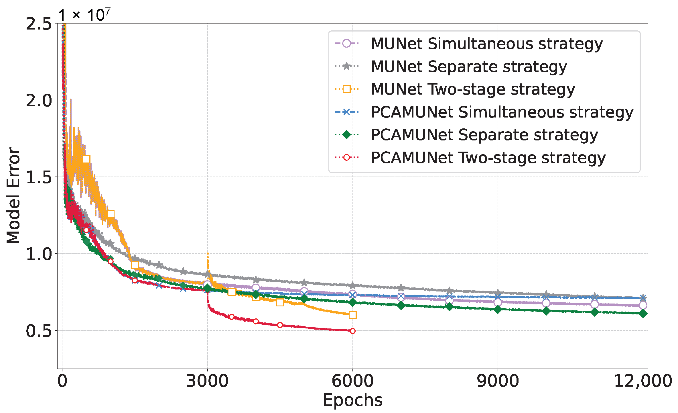
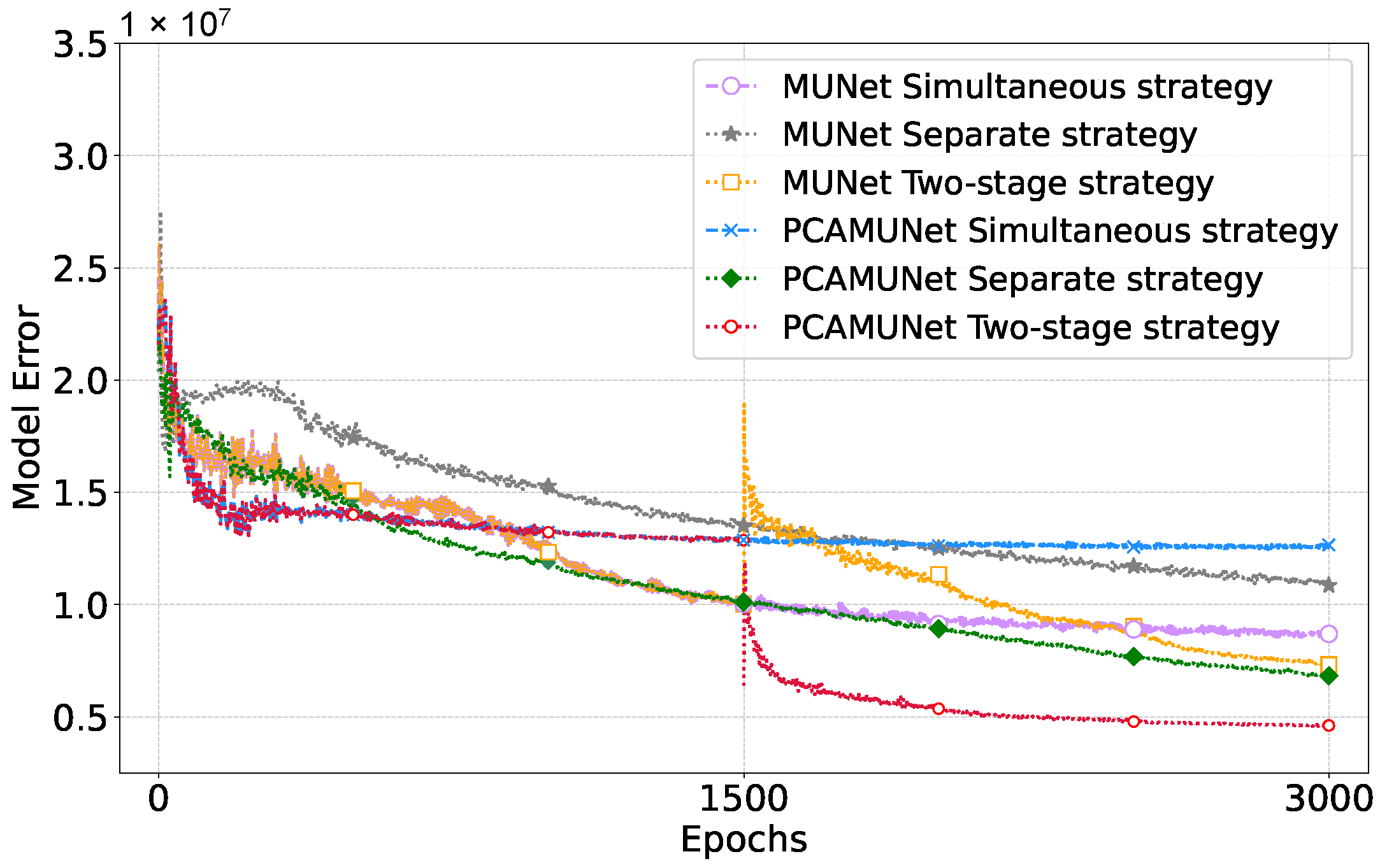
2.5. Two-Stage Training Strategy

Taking into account the impact of different forward simulations on the efficiency and accuracy of inversion, we design a two-stage training strategy. The workflow of the training process is depicted in Figure 4. For the two stages, the observed shot gathers both input separate shot gathers to the inversion network.

(1) Stage one (simultaneous sources): In the first stage, simultaneous sources are used to perform a single execution of the forward operator to generate a synthetic super-shot gather, which contains the information of all shots. This pretraining phase achieves the efficient learning of the network and accelerates the convergence speed. In this stage, we use the waveform loss with time weighting (Equation (4)) as the loss function:

$$L_{\mathrm{Sim}}=L_{\mathrm{Time}\mathrm{Waveform}}=\left|G\left(t\right)\left(\sum _{i=1}^n{Y}_i-\overline{Y}\right)\right|,$$

(7)

where n is the number of shots; $Y_i$ is the observed shot gather for the i-th shot, the observed super-shot record is generated by stacking all observed shot gathers; and $\overline{Y}$ is the synthetic super-shot gather using simultaneous sources.

(2) Stage two (separate sources): In the second stage, separate sources are employed to perform the forward operator as many times as the number of observed shots. The synthetic separate shot gathers help the network suppress the cross talks produced in the first stage to improve the inversion accuracy. In the second stage, the hybrid loss function, combing the waveform loss with time weighting and logarithmic envelope loss, is defined as follows:

$$\begin{array}{cc}\hfill L_{\mathrm{Sep}}& =\alpha L_{\mathrm{Time}\mathrm{Waveform}}+\beta L_{\mathrm{Log}\mathrm{Envelope}}\hfill \\ \hfill & =\alpha \sum _{i=1}^n\left(G\left(t\right)\left|Y_i-{\overline{\overline{Y}}}_i\right|\right)+\beta \sum _{i=1}^n\left|E_i-{\overline{\overline{E}}}_i\right|,\hfill \end{array}$$

(8)

where n is the total number of shots; $Y_i$ and ${\overline{\overline{Y}}}_i$ denote the observed and the synthetic shot gather for the i-th shot, respectively; $E_i$ and ${\overline{\overline{E}}}_i$ are the corresponding logarithmic envelope for the i-th shot gather, respectively; the weight parameters $\alpha$ and $\beta$ are used to balance the contributions of the different loss components. The waveform loss with time weighting focuses on discrepancies between time samples, while the logarithmic envelope loss captures the low-frequency waveform amplitude variations. By combining these two losses, the hybrid loss function improves the precision of the inversion in both time-resolution and amplitude, thereby enhancing the stability and accuracy of the inversion process.

For the network optimization, we employ the AdamW optimizer with an initial learning rate of 0.002. To enhance the learning of complex patterns, we implement a learning rate decay strategy [40], which reduces the learning rate by a factor of 0.6 at the 1000th and 2000th epochs. Meanwhile, we utilize the Kaiming initialization to initialize the parameters of the PCAMUNet. For hyperparameters a, $\alpha$, and $\beta$, we select $a=$ 0.5, $\alpha =$ 0.1, and $\beta =$ 0.9 as the optimal values in the ablation experiments. While the velocity model serve as the most direct criterion to determine the optimal hyperparameters, the shot gathers can also act as an indirect criterion when applied to field data.

2.6. Quantitative Indicators

This paper employs three metrics to comprehensively assess inversion performance:

• The normalized root mean square error (NRMSE, Equation (9)) quantifies absolute prediction errors normalized by the data range, with values closer to 0 indicating higher accuracy;
• The coefficient of determination (R², Equation (10)) measures explained variance (1 is optimal);
• The Pearson correlation coefficient (PCC, Equation (11)) measures linear trend consistency between predictions and labels, with values near ±1 reflecting strong linear trend consistency.

$$\mathrm{NRMSE}={\displaystyle \frac{\sqrt{\frac{1}{N}{\sum }_{i=1}^N{(a_i-{\tilde{a}}_i)}^2}}{a_{max}-a_{min}}},$$

(9)

$${\mathrm{R}}^2=1-{\displaystyle \frac{{\sum }_{i=1}^N{(a_i-{\tilde{a}}_i)}^2}{{\sum }_{i=1}^N{(a_i-\overline{a})}^2}},$$

(10)

$$\mathrm{PCC}={\displaystyle \frac{{\sum }_{i=1}^N\left(a_i-\overline{a}\right)\left({\tilde{a}}_i-\overline{\tilde{a}}\right)}{\sqrt{{\sum }_{i=1}^N{\left(a_i-\overline{a}\right)}^2}\sqrt{{\sum }_{i=1}^N{\left({\tilde{a}}_i-\overline{\tilde{a}}\right)}^2}}},$$

(11)

where N is the number of time samples; $a_i$ and ${\tilde{a}}_i$ denote the i-th label value and the output value, respectively; $a_{max}$ and $a_{min}$ are the maximum and minimum value of the label value, respectively; $\overline{a}$ and $\overline{\tilde{a}}$ are the average of the label value and the output value, respectively.

3. Experiments and Results

The numerical experiments conducted in this work involve three datasets: the Marmousi2 model [41], the Overthrust model, and the BP model [42]. In this section, we not only compare the MUNet with the proposed PCAMUNet, but also compare the proposed two-stage strategy with two single-stage strategies: the simultaneous source only with $L_{\mathrm{Sim}}$ (Equation (7)) strategy (simultaneous strategy) and the separate source only with $L_{\mathrm{Sep}}$ (Equation (8)) strategy (separate strategy). To better compare the effects of different network architectures and source training strategies on inversion results, we conducted experiments using the same observation system. The three velocity models are discretized with 256 grid points laterally and 128 grid points in depth, with a spatial sampling of 0.01 km in both directions. The time step is set to 0.001 s and the total simulation time is set to 2.048 s. The observation system is configured to a fixed spread geometry: 20 shots are evenly spaced along the surface from 0.04 to 2.52 km; receivers are placed at all grid points corresponding to a depth of 0.02 km, with a total of 256 receivers. The source is Ricker wavelet with a peak frequency of 8 Hz. All training is based on the Pytorch framework (1.12.1 (CUDA 11.3)) and utilizes the GeForce RTX 3090 GPU (NVIDIA Corporation, Xi’an, China) for acceleration.

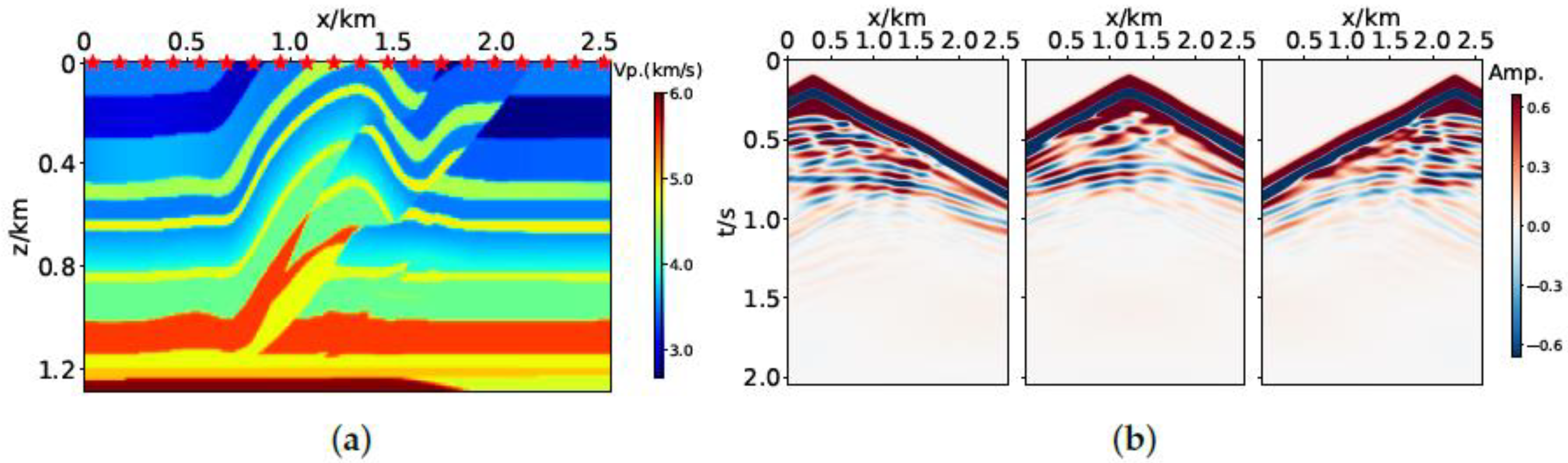
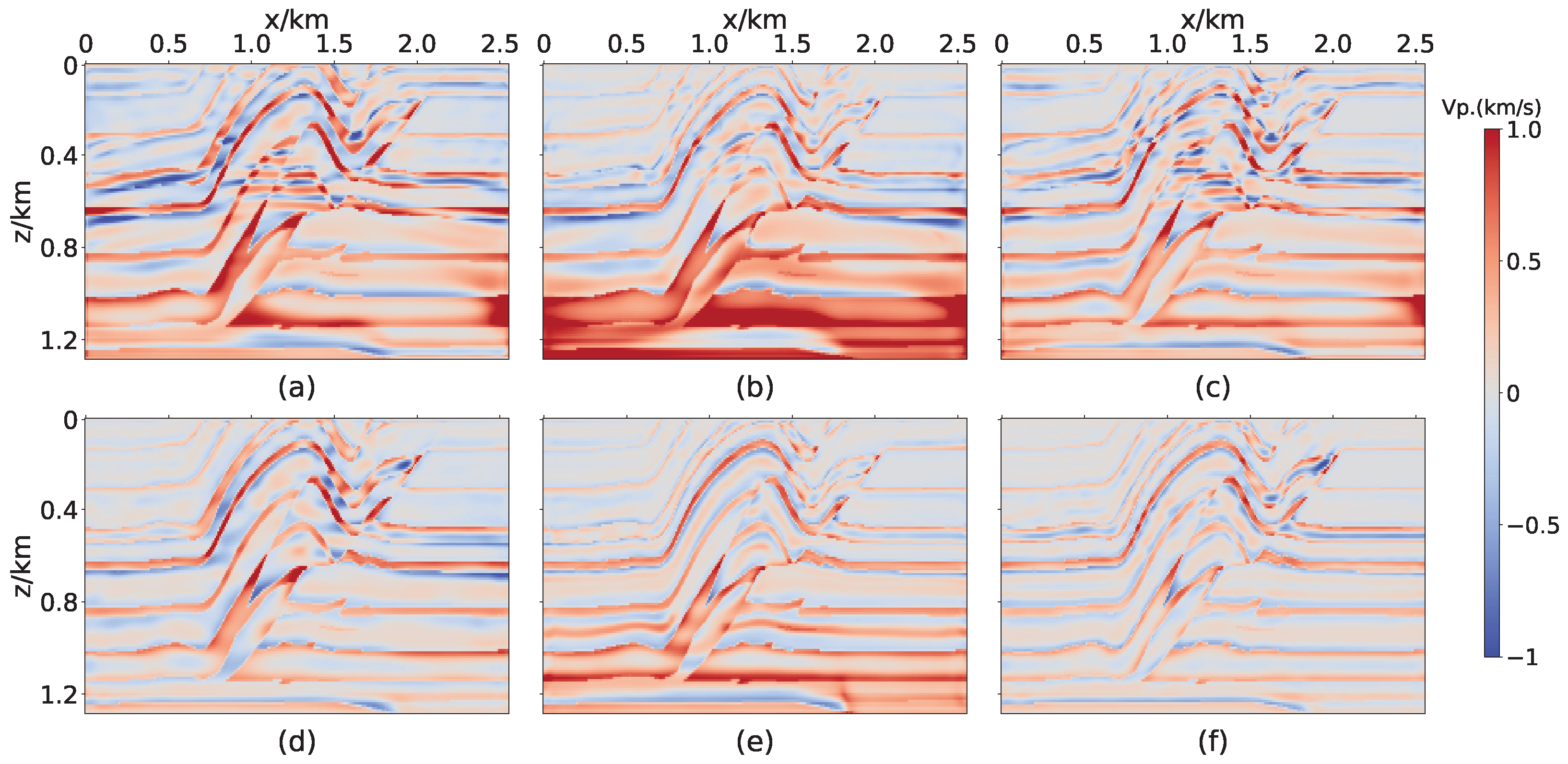
3.1. Marmousi2 Model

The Marmousi2 model serves as a benchmark geophysical model characterized by complex geological structures, including multiple faults, distinct interfaces, and significant lateral and vertical variations. We utilize the down-sampled Marmousi2 model to verify the reliability of the proposed two-stage FWI strategy. Figure 5a depicts the velocity model with seismic wave speeds ranging from 1480 to 4700 m/s and the red stars are the position of 20 shots. Figure 5b shows three representative shot records (the 3rd, 10th, and 18th) of the 20 shots, and Figure 5c shows a super-shot gather generated by a simultaneous source.

Each single-stage strategy is trained for 12,000 epochs, while the proposed two-stage involves training for 3000 epochs per stage. To ensure a fair comparison, we use the network parameters from the 3000th epoch of the simultaneous source as the result for our first stage. Subsequently, we apply a transfer learning strategy, initializing the second stage network parameters with those from the first stage, to expedite convergence.

Figure 6 displays the inversion results: MUNet in the top row and PCAMUNet in the bottom row. Each column represents the different training strategy: simultaneous strategy (left), separate strategy (middle), and the proposed two-stage strategy (right). On the one hand, compared with (a–c) predicted by MUNet, (d–f) show that the proposed PCAMUNet achieves significantly superior inversion accuracy. PCAMUNet reconstructs velocity models with higher resolution, particularly excelling at capturing complex boundaries and subtle structures of deep high-velocity formations. This enhancement stems from its PConv blocks and attention mechanisms, which strengthen edge-information extraction and critical geological feature identification. On the other hand, (a, d), lacking structure details, are the inversion results at the 12,000th epoch using simultaneous source only; (b, e), offering richer details but with the inaccurate prediction for layers in deep region, are the inversion results at the 12,000th epoch using separate source only. As for the proposed two-stage strategy, using simultaneous source for pretraining is crucial for initial iterations to quickly approximate the background velocity model. The inverted velocity model (Figure 6f) at the 6000th epoch is closest to the ground truth and has the richest details with the highest efficiency. Furthermore, the two-stage strategy with PCAMUNet effectively recovers both high-speed and low-speed layers with superior lateral continuity in mid-depth regions (black rectangular boxes). As indicated by the black arrows, this proposed method significantly enhances reconstruction of intricate structures in deeper areas.

Figure 7 illustrates the errors between the inversion results and the true velocity model. The errors reveal that the PCAMUNet-based strategies demonstrate significantly lower overall errors compared to the MUNet-based strategies, particularly in deep regions and complex structural areas. Notably, while both simultaneous source and separate source strategies perform comparably in shallow regions, the two-stage strategy exhibits markedly smaller errors in edge and deep regions than single-strategy methods, with the most uniform error distribution. This indicates its superior capability in characterizing high-contrast interfaces and velocity anomalies.

Figure 8 shows the model error curves of Marmousi2 model. It can be seen that the proposed two-stage strategy using PCAMUNet (red curve) not only has the fastest convergence speed but also the highest inversion accuracy.

Table 1. Quantitative comparison of inversion results on Marmousi2 model (best results are highlighted in bold).

Network	Strategy	NRMSE	R2	PCC	Training Time (s)
MUNet	Simultaneous	0.1115	0.8571	0.9323	1268
	Separate	0.1209	0.8320	0.9157	5538
	Two-stage	0.1004	0.8840	0.9456	1615
PCAMUNet	Simultaneous	0.0976	0.8905	0.9458	1796
	Separate	0.1018	0.8809	0.9411	7185
	Two-stage	0.0794	0.9275	0.9637	1787

confirms these findings quantitatively, showing that the two-stage PCAMUNet method yields the lowest NRMSE and highest R² and PCC values while requiring the shortest training time, thus outperforming all other tested methods.

3.2. Overthrust Model

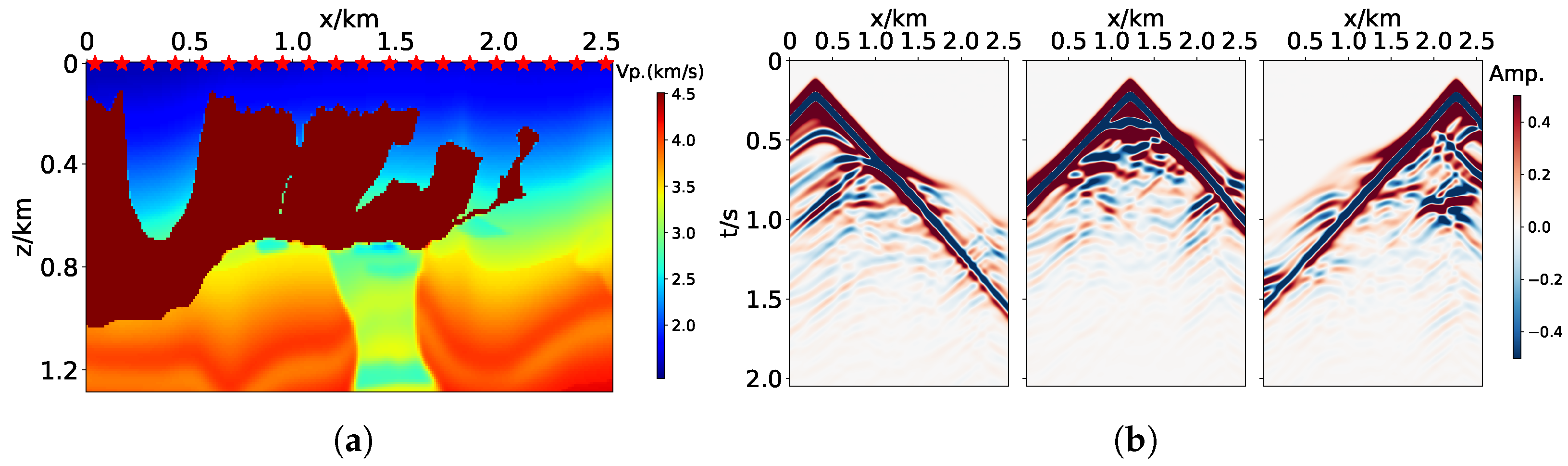
The Overthrust model is employed as an additional testing model to further validate the effectiveness of the proposed method. The Overthrust model is particularly suitable for testing stability in regions with steep velocity gradients, making it a critical test model for evaluating the geological structure recovery capabilities of inversion methods. In Figure 9a, the velocity range of this resized version of the overthrust model spans from 2670 to 6000 m/s and the red stars are the position of 20 shots. Figure 9b displays the 3rd, 10th, and 18th shots among the 20 total gathers.

Considering that the structure of the Overthrust model is simpler than that of the Marmousi2 model, each single-stage strategy is trained for 3000 epochs, while the proposed two-stage strategy involves training for 1500 epochs per stage. Figure 10 shows the inversion results. On the one hand, compared to Figure 10a–c predicted by MUNet, Figure 10d–f also show that the proposed PCAMUNet can significantly improve the inversion accuracy. On the other hand, compared to both Figure 10d,e predicted by single-stage strategy, Figure 10f demonstrates superior fidelity to the ground truth and successfully recovers both low- and high-velocity layers. Furthermore, the two-stage strategy is also observed to effectively recover both the high-speed and low-speed layer, as indicated by the black rectangular boxes, while Figure 10e has inaccurate predictions in red rectangular boxes. Additionally, the black arrows also highlight that the two-stage strategy using PCAMUNet enhances the ability to reconstruct the intricate structures found in the fault region. Figure 11 presents the errors between each result and the true velocity model, where lighter color intensities indicate smaller deviations from the labeled model. Notably, Figure 11f exhibits the lightest color map and the most homogeneous color distribution, demonstrating that the proposed method efficiently reconstructs both the layered structures and velocity anomalies present in the Overthrust model.

Furthermore, to evaluate the convergence performance of different methods, Figure 12 depicts the velocity model error curves throughout the training process. The results clearly demonstrate that the proposed inversion method achieves the highest inversion accuracy with the same number of training iterations as competing methods. For the quantitative comparison presented in

Table 2. Quantitative comparison of the inversion results on the overthrust model (best results are highlighted in bold).

Network	Strategy	NRMSE	R2	PCC
MUNet	Simultaneous	0.1091	0.7905	0.8992
	Separate	0.1421	0.6446	0.8643
	Two-stage	0.0924	0.8496	0.9291
PCAMUNet	Simultaneous	0.0779	0.8933	0.9470
	Separate	0.0865	0.8682	0.9440
	Two-stage	0.0616	0.9331	0.9667

, the proposed network with the two-stage strategy achieves an optimal performance across all evaluation metrics.

3.3. BP Model

To further investigate the robustness and generalization, we provide experimental results on part of the resized BP model here to demonstrate the effectiveness of the proposed method. The red stars are the position of 20 shots, and the experiment extracts the left region of the BP model containing typical salt dome structures, with velocities ranging from 1574 to 4510 m/s, as illustrated in Figure 13a. Figure 13b displays the 3rd, 10th, and 18th shot records from the observed gathers.

Each single-stage strategy is trained for 4000 epochs, while the proposed two-stage strategy involves training for 2000 epochs per stage. The inversion results are shown in Figure 14. Compared to the inversion results predicted by the MUNet network (Figure 14a–c), the proposed PCAMUNet method (Figure 14d–f) yields significantly higher quality reconstructions. Furthermore, the MUNet-based methods exhibit noticeable waveform information residuals in the regions indicated by black arrows, demonstrating that PCAMUNet effectively processes the relationship between seismic shot gather features and velocity model characteristics. Figure 14a,d do not capture the structure beneath the salt body. Additionally, Figure 14f predicted by the PCAMAUNet with the two-stage strategy is closest to the ground truth, while Figure 14b,c,e fail to capture the structure in the black rectangular boxes. The proposed method more accurately delineates salt body boundaries with sharper transitions and geometric morphologies closer to the true model.

Figure 15 shows the model error curves of the BP model. Upon the completion of 4000 training epoch, the two-stage strategy with PCAMUNet delivers the highest precision in inversion results.

Table 3. Quantitative comparison of inversion results on BP model (best results are highlighted in bold).

Network	Strategy	NRMSE	R2	PCC
MUNet	Simultaneous	0.2405	0.5153	0.7746
	Separate	0.1174	0.8845	0.9482
	Two-stage	0.1059	0.9060	0.9572
PCAMUNet	Simultaneous	0.1645	0.7734	0.8887
	Separate	0.1058	0.9063	0.9596
	Two-stage	0.0745	0.9535	0.9788

summarizes the quantitative performance metrics for all methods. The proposed two-stage strategy with PCAMAUNet demonstrates an exceptional performance across all evaluation criteria. As with the conclusion of the Marmousi2 and Overthrust model, the two-stage strategy with PCAMUNet stands out for its superior efficiency.

4. Discussion

Based on the experimental analysis above, we can conclude that the proposed method can improve the inversion results in both the Marmousi2, the Overthrust, and the BP models. Since these experiments are conducted under ideal conditions, we further investigate how noise and missing low-frequency components in observed seismic data affect the inversion performance. For comparison, a traditional multiscale FWI methodology is employed as a baseline approach in the stress tests. The multiscale FWI follows a low-to-high frequency multiscale strategy, employing gradient descent to iteratively update velocity models, representing the current mainstream approach in conventional FWI. The implementation of the multiscale FWI uses five frequency bands ranging from 3 Hz to 15 Hz (3 Hz, 5 Hz, 8 Hz, 12 Hz, and 15 Hz) with 100 iterations per band, employing the LBFGS optimizer with a strong Wolfe line search adopted to ensure convergence.

As for the noise perturbation experiments, Figure 16 illustrates three (the 3rd, 10th, and 18th) shot gathers with Gaussian noise ($\sigma =0.5{\sigma }_0$), where $\sigma$ represents the variance of the noise and ${\sigma }_0$ denotes the variance of the clean seismic data. Figure 17 illustrates the velocity models predicted by traditional multiscale FWI and PCAMUNet with the two-stage strategy under the influence of noisy observed shot gathers. The experimental results clearly demonstrate that the two-stage PCAMUNet exhibits superior noise resistance, successfully inverting the structural information of the velocity model.

As for the missing low-frequency experiment, Figure 18a displays the original observed shot gather, the filtered shot gather after applying a high-pass filter to attenuate frequencies starting from 5 Hz, and the corresponding difference. The central shot is selected for comparison. Figure 18b shows the amplitude spectra of the shot gathers for comparison.

Figure 19 shows the velocity models predicted under the influence of observed shot gathers with missing low-frequency information using traditional multiscale FWI (Figure 19a), the PCAMUNet network with two stages but based on waveform loss with time weighting (Figure 19b), and the proposed PCAMUNet with the two-stage strategy (Figure 19c). Result (Figure 19b)demonstrates that the two-stage strategy performs effectively even when low-frequency information is absent from the observed marine data, as long as waveform-based loss is utilized during training. Moreover, Figure 19c demonstrates that the proposed hybrid loss, combining both waveform-based and envelope-based losses, achieves better accuracy, particularly recovering high-velocity structures. Furthermore, compared to traditional multiscale FWI, the proposed method produces results closer to the true values and better handles structural details in edge regions, as shown in the areas marked by black rectangles.

In the proposed approach, the primary computational burden comes from the forward modeling of the data, but we have implemented the two-stage strategy to enhance the overall efficiency. Specifically, during the first stage (simultaneous source), each iteration only requires modeling one super-shot rather than individual shots, significantly reducing the per-iteration cost. Moreover, our approach leverages the simultaneous source inversion to provide a high-quality initial model for the subsequent second stage (separate source), thereby reducing the total number of iterations needed in the more expensive stage. While the current approach already improves computational efficiency compared to conventional FWI, we acknowledge that further optimizations could be explored to reduce costs even more, such as low-rank decomposition-based reparameterization [43] or advanced network architectures.

The physics-guided self-supervised learning method proposed in this work provides a flexible training strategy for FWI, incorporating a designed loss function and an innovative two-stage training strategy. These core strategic elements possess a modular nature, enabling them not only to perform FWI tasks effectively on their own but also to be readily integrated or combined with other emerging physics-informed machine learning frameworks (such as PINNs, operator learning, or hybrid inversion strategies). For instance, our method employs distinct loss functions in different stages and a two-stage training methodology involving initial pretraining with simultaneous sources followed by fine-tuning using separate shot gathers. This strategy is designed to efficiently construct background velocity models and accurately recover fine-scale details. The underlying concept could offer an optimization pathway for other computationally intensive learning tasks, aiding in balancing computational efficiency with model accuracy. The key of the proposed training strategy lies in its adherence to physical laws for self-supervised learning, positioning it as a potentially valuable complement to existing physics-informed learning approaches.

Looking forward, generalizing this training strategy to three-dimensional (3D) FWI is crucial for enhancing its practical value, despite the significant challenges posed by computational cost and memory requirements. The fundamental principles of our method in principle can be extended to 3D scenarios. However, its training procedures and network architecture require further optimization for the characteristics of 3D seismic data. This includes, for instance, investigating more efficient 3D simultaneous-source encoding techniques with a 3D differentiable solver to balance efficiency and accuracy. Future research will focus on improving computational feasibility and inversion quality in 3D applications. Promising avenues include the exploration of data compression techniques and more memory-efficient network parameterizations (such as deep image prior (DIP) or implicit neural representations (INRs)), aiming to leverage the advantages of our strategy in large-scale 3D seismic inversion.

5. Conclusions

We proposed a two-stage self-supervised FWI strategy, effectively combining computational efficiency with inversion accuracy. PCAMUNet successfully achieves high-precision mapping from shot gather data to velocity model. The network utilizes PConv to replace Conv and introduces AG and SE modules, significantly enhancing the extraction capability of key features from seismic data. In terms of training strategy, this paper innovatively designs a two-stage strategy. The inversion network is pretrained by the forward operator with a simultaneous source in the first stage. The pretraining phase enables the network to learn efficiently using a loss function based on waveform loss with time weighting. Then, each shot is forward modeled individually using a separate source in the second stage, allowing the network to learn high precision information with the hybrid loss function combining waveform with time weighting and logarithmic envelope loss. By first performing a coarser inversion in the first stage to obtain the background velocity model, the second stage can more quickly optimize the velocity model, significantly reducing the overall training time. With the forward operator, the inversion framework enables the inversion process to adhere to the physics law and avoid the use of the labeled velocity model. Experiments conducted on the Marmousi2, Overthrust, and BP model demonstrate that the proposed two-stage strategy markedly improves the inversion performance, yielding accurate inversion results with rapid convergence. Additionally, noise resistance experiments and low-frequency missing experiments prove that the proposed strategy exhibits superior noise resistance and stability when a low-frequency data component is missing.

References

1. Tarantola, A. Inversion of seismic reflection data in the acoustic approximation. Geophysics 1984, 49, 1259–1266. [Google Scholar] [CrossRef]
2. LeCun, Y.; Bengio, Y.; Hinton, G. Deep learning. Nature 2015, 521, 436–444. [Google Scholar] [CrossRef]
3. Anjom, F.K.; Vaccarino, F.; Socco, L.V. Machine learning for seismic exploration: Where are we and how far are we from the holy grail? Geophysics 2024, 89, WA157–WA178. [Google Scholar] [CrossRef]
4. Zhang, Z.D.; Alkhalifah, T. Regularized elastic full waveform inversion using deep learning. Geophysics 2019, 84, R741–R751. [Google Scholar] [CrossRef]
5. Sun, B.; Alkhalifah, T. ML-descent: An optimization algorithm for full-waveform inversion using machine learning. Geophysics 2020, 85, R477–R492. [Google Scholar] [CrossRef]
6. Zhang, Z.d.; Alkhalifah, T. High-resolution reservoir characterization using deep learning-aided elastic full-waveform inversion: The North Sea field data example. Geophysics 2020, 85, WA137–WA146. [Google Scholar] [CrossRef]
7. Yang, F.; Ma, J. Deep-learning inversion: A next-generation seismic velocity model building method. Geophysics 2019, 84, R583–R599. [Google Scholar] [CrossRef]
8. Wu, Y.; Lin, Y. InversionNet: An efficient and accurate data-driven full waveform inversion. IEEE Trans. Comput. Imaging 2019, 6, 419–433. [Google Scholar] [CrossRef]
9. Zhang, Z.; Wu, Y.; Zhou, Z.; Lin, Y. VelocityGAN: Subsurface velocity image estimation using conditional adversarial networks. In Proceedings of the 2019 IEEE Winter Conference on Applications of Computer Vision (WACV), Waikoloa, HI, USA, 7–11 January 2019; pp. 705–714. [Google Scholar]
10. Li, F.; Guo, Z.; Pan, X.; Liu, J.; Wang, Y.; Gao, D. Deep learning with adaptive attention for seismic velocity inversion. Remote Sens. 2022, 14, 3810. [Google Scholar] [CrossRef]
11. Li, H.; Li, J.; Li, X.; Dong, H.; Xu, G.; Zhang, M. MAU-Net: A multi-branch attention U-Net for full-wavefom inversion. Geophysics 2024, 89, R119–R216. [Google Scholar] [CrossRef]
12. Feng, S.; Lin, Y.; Wohlberg, B. Multiscale data-driven seismic full-waveform inversion with field data study. IEEE Trans. Geosci. Remote Sens. 2021, 60, 4506114. [Google Scholar] [CrossRef]
13. Ovcharenko, O.; Kazei, V.; Alkhalifah, T.A.; Peter, D.B. Multi-task learning for low-frequency extrapolation and elastic model building from seismic data. IEEE Trans. Geosci. Remote Sens. 2022, 60, 4510717. [Google Scholar] [CrossRef]
14. Saadat, M.; Hashemi, H.; Nabi-Bidhendi, M. Generalizable data driven full waveform inversion for complex structures and severe topographies. Pet. Sci. 2024, 21, 4025–4033. [Google Scholar] [CrossRef]
15. Gao, Z.; Yang, W.; Li, C.; Li, F.; Wang, Q.; Ding, J.; Gao, J.; Xu, Z. Self-supervised deep learning for nonlinear seismic full waveform inversion. IEEE Trans. Geosci. Remote Sens. 2022, 60, 4509518. [Google Scholar] [CrossRef]
16. Feng, Y.; Chen, Y.; Jin, P.; Feng, S.; Liu, Z.; Lin, Y. Simplifying full waveform inversion via domain-independent self-supervised learning. arXiv 2023, arXiv:2305.13314. [Google Scholar]
17. Sun, J.; Innanen, K.; Zhang, T.; Trad, D. Implicit seismic full waveform inversion with deep neural representation. J. Geophys. Res. Solid Earth 2023, 128, e2022JB025964. [Google Scholar] [CrossRef]
18. Yang, F.; Ma, J. FWIGAN: Full-Waveform Inversion via a Physics-Informed Generative Adversarial Network. J. Geophys. Res. Solid Earth 2023, 128, e2022JB025493. [Google Scholar] [CrossRef]
19. Song, C.; Alkhalifah, T.A. Wavefield reconstruction inversion via physics-informed neural networks. IEEE Trans. Geosci. Remote Sens. 2021, 60, 5908012. [Google Scholar] [CrossRef]
20. Dhara, A.; Sen, M.K. Physics-guided deep autoencoder to overcome the need for a starting model in full-waveform inversion. Lead. Edge 2022, 41, 375–381. [Google Scholar] [CrossRef]
21. Jin, P.; Zhang, X.; Chen, Y.; Huang, S.X.; Liu, Z.; Lin, Y. Unsupervised Learning of Full-Waveform Inversion: Connecting CNN and Partial Differential Equation in a Loop. arXiv 2022, arXiv:2110.07584. [Google Scholar] [CrossRef]
22. Liu, B.; Jiang, P.; Wang, Q.; Ren, Y.; Yang, S.; Cohn, A.G. Physics-driven self-supervised learning system for seismic velocity inversion. Geophysics 2023, 88, R145–R161. [Google Scholar] [CrossRef]
23. Muller, A.P.; Costa, J.C.; Bom, C.R.; Klatt, M.; Faria, E.L.; de Albuquerque, M.P.; de Albuquerque, M.P. Deep pre-trained FWI: Where supervised learning meets the physics-informed neural networks. Geophys. J. Int. 2023, 235, 119–134. [Google Scholar] [CrossRef]
24. Mustajab, A.H.; Lyu, H.; Rizvi, Z.; Wuttke, F. Physics-informed neural networks for high-frequency and multi-scale problems using transfer learning. Appl. Sci. 2024, 14, 3204. [Google Scholar] [CrossRef]
25. Shin, C.; Cha, Y.H. Waveform inversion in the Laplace domain. Geophys. J. Int. 2008, 173, 922–931. [Google Scholar] [CrossRef]
26. Alkhalifah, T.; Song, C. An efficient wavefield inversion: Using a modified source function in the wave equation. Geophysics 2019, 84, R909–R922. [Google Scholar] [CrossRef]
27. Bozdağ, E.; Trampert, J.; Tromp, J. Misfit functions for full waveform inversion based on instantaneous phase and envelope measurements. Geophys. J. Int. 2011, 185, 845–870. [Google Scholar] [CrossRef]
28. Du, M.; Cheng, S.; Mao, W. Deep-learning-based seismic variable-size velocity model building. IEEE Geosci. Remote Sens. Lett. 2022, 19, 3008305. [Google Scholar] [CrossRef]
29. Sun, B.; Alkhalifah, T. ML-misfit: A neural network formulation of the misfit function for full-waveform inversion. Front. Earth Sci. 2022, 10, 1011825. [Google Scholar] [CrossRef]
30. Saad, O.M.; Harsuko, R.; Alkhalifah, T. SiameseFWI: A deep learning network for enhanced full waveform inversion. J. Geophys. Res. Mach. Learn. Comput. 2024, 1, e2024JH000227. [Google Scholar] [CrossRef]
31. Xu, Z.Q.J.; Zhang, Y.; Luo, T.; Xiao, Y.; Ma, Z. Frequency principle: Fourier analysis sheds light on deep neural networks. arXiv 2019, arXiv:1901.06523. [Google Scholar]
32. Zhu, W.; Xu, K.; Darve, E.; Biondi, B.; Beroza, G.C. Integrating deep neural networks with full-waveform inversion: Reparameterization, regularization, and uncertainty quantification. Geophysics 2022, 87, R93–R109. [Google Scholar] [CrossRef]
33. Liu, G.; Shih, K.J.; Wang, T.C.; Reda, F.A.; Sapra, K.; Yu, Z.; Tao, A.; Catanzaro, B. Partial convolution based padding. arXiv 2018, arXiv:1811.11718. [Google Scholar]
34. Oktay, O.; Schlemper, J.; Folgoc, L.L.; Lee, M.; Heinrich, M.; Misawa, K.; Mori, K.; McDonagh, S.; Hammerla, N.Y.; Kainz, B.; et al. Attention u-net: Learning where to look for the pancreas. arXiv 2018, arXiv:1804.03999. [Google Scholar]
35. Hu, J.; Shen, L.; Sun, G. Squeeze-and-excitation networks. In Proceedings of the IEEE Conference on Computer Vision and Pattern Recognition, Salt Lake City, UT, USA, 18–23 June 2018; pp. 7132–7141. [Google Scholar]
36. Richardson, A. Deepwave. Zenodo 2023. [Google Scholar] [CrossRef]
37. Wu, R.S.; Luo, J.; Wu, B. Seismic envelope inversion and modulation signal model. Geophysics 2014, 79, WA13–WA24. [Google Scholar] [CrossRef]
38. Cheng, Q. Digital Signal Processing; Peking University Press: Beijing, China, 2010; pp. 137–141. [Google Scholar]
39. Bao, Q.; Chen, J.; Wu, H. Multi-scale full waveform inversion based on logarithmic envelope of seismic data. Geophys. Prospect. Pet. 2018, 57, 584–591. [Google Scholar]
40. You, K.; Long, M.; Wang, J.; Jordan, M.I. How does learning rate decay help modern neural networks? arXiv 2019, arXiv:1908.01878. [Google Scholar]
41. Martin, G.S.; Wiley, R.; Marfurt, K.J. Marmousi2: An elastic upgrade for Marmousi. Lead. Edge 2006, 25, 156–166. [Google Scholar] [CrossRef]
42. Billette, F.; Brandsberg-Dahl, S. The 2004 BP velocity benchmark. In Proceedings of the 67th EAGE Conference & Exhibition, Madrid, Spain, 13–16 June 2005; European Association of Geoscientists & Engineers: Utrecht, The Netherlands, 2005; p. cp–1–00513. [Google Scholar]
43. Luo, Y.; Zhao, X.; Li, Z.; Ng, M.K.; Meng, D. Low-rank tensor function representation for multi-dimensional data recovery. IEEE Trans. Pattern Anal. Mach. Intell. 2023, 46, 3351–3369. [Google Scholar] [CrossRef]
Figure 1. Scheme of the physics-guided self-supervised inversion framework. The process begins with the multi-channel observed shot gathers which are input into the inversion network to predict a velocity model. Then, the predicted velocity model is fed into a wave equation to generate the corresponding synthetic shot gathers. The update process is completed through backpropagation, which utilizes the gradient of the loss function that evaluates the difference between observed and synthetic data.
Jmse 13 01193 g001
Figure 2. Visualization of X, 1, X p 0 , 1 p 0 , and 1 p 1 . The red and green boxes are the sliding convolution window examples centering at position ( i , j ) .
Jmse 13 01193 g002
Figure 3. The PConv attention modified UNet (PCAMUNet) architecture for FWI. The numbers above the cubes represent the number of channels in the feature maps at each level. The architecture takes multichannel shot gathers as input and outputs a velocity model. With PConv layers and two attention mechanisms—attention gate (AG) and squeeze-and-excitation (SE)—PCAMUNet can extract distinct features representing the velocity model.
Jmse 13 01193 g003
Figure 4. Workflow of the two-stage training strategy for the proposed FWI.
Jmse 13 01193 g004
Figure 5. Marmousi2 P-wave velocity model and observed shot gathers. (a) Marmousi2 model. (b) Three representative shot gathers (the 3rd, 10th, and 18th shots). and (c) Super-shot gather.
Jmse 13 01193 g005
Figure 6. Inversion results of Marmousi2 model. Top row: inverted Vp of MUNet with (a) simultaneous strategy; (b) separate strategy; (c) two-stage strategy; Bottom row: inverted Vp of PCAMUNet with (d) simultaneous strategy, (e) separate strategy, and (f) two-stage strategy.
Jmse 13 01193 g006
Figure 7. Inversion errors of Marmousi2 model. Top row: inverted Vp of MUNet with the (a) simultaneous strategy, (b) separate strategy, (c) two-stage strategy; Bottom row: inverted Vp of PCAMUNet with (d) simultaneous strategy, (e) separate strategy, (f) two-stage strategy.
Jmse 13 01193 g007
Figure 8. The model error curves on Marmousi2 model test. Each curve accounts for different training strategies using different network: the purple curve is a simultaneous strategy using MUNet; the gray curve is a separate strategy using MUNet; the orange curve is a two-stage strategy using MUNet; the blue curve is a simultaneous strategy using PCAMUNet; the green curve is a separate strategy using PCAMUNet; the red curve is the proposed two-stage strategy using PCAMUNet.
Jmse 13 01193 g008
Figure 9. Overthrust P-wave velocity model and observed shot gathers. (a) Overthrust model. (b) Three representative shot gathers (the 3rd, 10th, and 18th shots).
Jmse 13 01193 g009
Figure 10. Inversion results of the Overthrust model. Top row: inverted Vp of MUNet with (a) simultaneous strategy, (b) separate strategy, (c) two-stage strategy; Bottom row: inverted Vp of PCAMUNet with (d) simultaneous strategy, (e) separate strategy, (f) two-stage strategy.
Jmse 13 01193 g010
Figure 11. Inversion errors of the Overthrust model. Top row: inverted Vp of MUNet with (a) simultaneous strategy, (b) separate strategy, (c) two-stage strategy; Bottom row: inverted Vp of PCAMUNet with (d) simultaneous strategy, (e) separate strategy, (f) two-stage strategy.
Jmse 13 01193 g011
Figure 12. The model error curves on the Overthrust model test. Each curve accounts for different training strategies using different network: the purple curve is simultaneous strategy using MUNet; gray curve is separate strategy using MUNet; the orange curve is the two-stage strategy using MUNet; the blue curve is a simultaneous strategy using PCAMUNet; the green curve is separate strategy using PCAMUNet; and the red curve is the proposed two-stage strategy using PCAMUNet.
Jmse 13 01193 g012
Figure 13. BP P-wave velocity model and observed shot gathers. (a) BP model. (b) Three representative shot gathers (the 3rd, 10th, and 18th shots).
Jmse 13 01193 g013
Figure 14. Inversion results of the BP model. Top row: inverted Vp of MUNet with (a) simultaneous strategy, (b) separate strategy, (c) two-stage strategy; Bottom row: inverted Vp of PCAMUNet with (d) simultaneous strategy, (e) separate strategy, (f) two-stage strategy.
Jmse 13 01193 g014
Figure 15. The model error curves on the BP model test. Each curve accounts for different training strategies using different networks: the purple curve is a simultaneous strategy using MUNet; the gray curve is a separate strategy using MUNet; the orange curve is a two-stage strategy using MUNet; the blue curve is a simultaneous strategy using PCAMUNet; the green curve is a separate strategy using PCAMUNet; and the red curve is the proposed two-stage strategy using PCAMUNet.
Jmse 13 01193 g015
Figure 16. Three (the 3rd, 10th, and 18th) representatives of 20 shot gathers under Gaussian noise ( σ = 0.5 σ 0 ).
Jmse 13 01193 g016
Figure 17. Inversion results of Marmousi2 model under the interference of Gaussian noise ( σ = 0.5 σ 0 ). (a) Traditional multiscale FWI. (b) Stage one (simultaneous source) with PCAMUNet. (c) Stage two (separate source) with PCAMUNet.
Jmse 13 01193 g017
Figure 18. Comparison between shot gathers. (a) (Left) The original observed shot gather; (middle) The filtered shot gather after applying a high-pass filter to attenuate frequencies start from 5 Hz; (Right) The residual. (b) Amplitude spectra of the original seismic data (blue curve) and the filtered data attenuate low-frequency information (red curve).
Jmse 13 01193 g018
Figure 19. Inversion results of the Marmousi2 model without low-frequency information in the observed data. (a) Traditional multiscale FWI. (b) PCAMUNet network with two-stage but based on waveform loss with time weighting. (c) PCAMUNet network with the proposed two-stage strategy.
Jmse 13 01193 g019