Elastic Wave Phase Inversion in the Local-Scale Frequency–Wavenumber Domain with Marine Towed Simultaneous Sources

Abstract

Elastic full waveform inversion (EFWI) is a crucial technique for retrieving high-resolution multi-parameter information. However, the lack of low-frequency components in seismic data may induce severe cycle-skipping phenomena in elastic full waveform inversion (EFWI). Recognizing the approximately linear relationship between the phase components of seismic data and the properties of subsurface media, we propose an Elastic Wave Phase Inversion in local-scale frequency–wavenumber domain (LFKEPI) method. This method aims to provide robust initial velocity models for EFWI, effectively mitigating cycle-skipping challenges. In our approach, we first employ a two-dimensional sliding window function to obtain local-scale seismic data. Following this, we utilize two-dimensional Fourier transforms to generate the local-scale frequency–wavenumber domain seismic data, constructing a corresponding elastic wave phase misfit. Unlike the Elastic Wave Phase Inversion in the frequency domain (FEPI), the local-scale frequency–wavenumber domain approach accounts for the continuity of seismic events in the spatial domain, enhancing the robustness of the inversion process. We subsequently derive the gradient operators for the LFKEPI methodology. Testing on the Marmousi model using a land seismic acquisition system and a simultaneous-source marine towed seismic acquisition system demonstrates that LFKEPI enables the acquisition of reliable initial velocity models for EFWI, effectively mitigating the cycle-skipping problem.

1. Introduction

The seismic velocity parameters are crucial for improving seismic migration and geological interpretation [1,2,3,4]. Full waveform inversion (FWI) is designed to obtain high-resolution estimations of subsurface physical properties by minimizing a misfit. However, FWI is inherently a nonlinear optimization problem, and the quality of the final inversion outcomes is highly influenced by the low-frequency data and initial models [5,6,7]. Unfortunately, 0–4 Hz seismic data are often contaminated by noise, and, in some cases, it is impossible to acquire effective low-frequency signals, which poses considerable challenges for the practical application of FWI [8,9]. Moreover, Crase et al. [10] found that the elastic full waveform inversion (EFWI) is more susceptible to cycle skipping compared to acoustic FWI. This issue arises primarily because the elastic wavefield must consider both P-wave and S-wave kinematics and dynamics, resulting in a more complex seismic wavefield that is prone to misalignments in waveform matching. In contrast, acoustic FWI mainly focuses on inverting P-wave velocity. EFWI, however, effectively reconstructs both P-wave and S-wave velocity parameters and even accommodates anisotropic parameters, providing a refined representation of subsurface wave propagation mechanisms [11]. Therefore, accurately recovering the P-wave and S-wave velocity information is essential for understanding wave propagation and achieving high-resolution imaging.

In recent years, many researchers have extensively studied the nonlinear issues of the FWI misfit. For example, the multiscale strategy begins by using the low-frequency information of seismic data to obtain the macro-scale information of the geological structures, gradually increasing the inversion frequency of seismic data, thereby facilitating convergence of the misfit to a global minimum [12,13,14,15]. To retrieve low-wavenumber information of the subsurface velocity model, Shin and Cha [16] leveraged zero-frequency information derived from the Laplace domain. This approach enabled the reconstruction of macro-structures of the subsurface velocity models, thereby offering a good initial model for FWI [17,18]. Furthermore, methods based on the envelope signals of seismic data can also effectively mitigate the nonlinearity of the misfit. For example, Wu et al. [6] and Chi et al. [19] noted that envelope operators serve as a nonlinear signal demodulation technique that can obtain numerical low-frequency seismic data, demonstrating that the demodulated low-frequency components correlate well with the low-wavenumber information of the subsurface structures [20,21,22,23,24,25,26]. The phases of seismic data primarily reflect the kinematic properties of seismic waves. In contrast to amplitude data, phase information shows a better linear relationship with subsurface parameters. Consequently, within the theoretical framework of FWI, developing a phase misfit is crucial for generating a reliable initial velocity model [27,28,29]. In the frequency domain, the seismic data phases can be naturally separated from the amplitude information and show high computational efficiency. However, with the rapid advancement of computer performance, time-domain FWI methods have emerged as more convenient for the data preprocessing and validation of inversion results, presenting substantial advantages for methods based on time-domain seismic data.

Furthermore, full waveform inversion (FWI) approaches that develop phase misfits can also employ wave equations in the time domain. For example, seismic data may be converted into the frequency domain, where the observed amplitude can be substituted for the synthetic amplitude before reverting to the time domain. This process results in a misfit that encompasses only the phase differences [30,31,32]. Fichtner et al. [33] proposed a time-frequency domain phase inversion method, which utilizes Gabor transforms to generate a time-frequency domain phase misfit, ultimately yielding favorable inversion results. Luo et al. [28] developed a misfit using instantaneous phase and employed an exponential damping to establish initial velocity models for EFWI. Hu et al. [34] introduced a phase cross-correlation algorithm that further mitigates the influence of amplitude information on inversion results. Kang et al. [35] introduced a frequency–wavenumber domain phase inversion method that effectively integrates the acoustic wave equation to achieve improved initial velocity models for FWI. Beyond traditional phase inversion techniques, recent advancements, such as adaptive FWI and phase correction methodologies, also address phase mismatch issues and contribute to the refinement of initial velocity models for FWI [36,37,38,39]. Consequently, FWI methods that utilize phase information for constructing misfits present distinct advantages in enhancing the precision of subsurface velocity inversion.

To achieve high-resolution inversion results for subsurface velocity models, we present an Elastic Wave Phase Inversion in the local-scale frequency–wavenumber domain (LFKEPI) method, which fully considers the local variation characteristics of seismic data in both time and offset directions. By combining local-scale transformations of seismic data with two-dimensional Fourier transforms, this method constructs a frequency–wavenumber domain phase misfit, providing a robust initial velocity model for the EFWI process. The structure of this paper is as follows: we begin by introducing the fundamental principles of EFWI. Next, we explore Elastic Wave Phase Inversion in the frequency domain (FEPI) method and present a comprehensive derivation of the adjoint source. Following this, we discuss the misfit and gradient operators specific to the LFKEPI method. Finally, we show some numerical tests on the Marmousi model.

2. Methodology of Elastic Parameter Inversion

2.1. Review of Elastic Full Waveform Inversion

The second-order partial differential equations of elastic wave propagation in two dimensions can be represented in the following format:

$$\left\{\begin{array}{l}\rho {\displaystyle \frac{{\partial }^2{u}_x}{\partial t^2}}={\displaystyle \frac{\partial {\sigma }_{xx}}{\partial x}}+{\displaystyle \frac{\partial {\sigma }_{xz}}{\partial z}}\\ \rho {\displaystyle \frac{{\partial }^2{u}_z}{\partial t^2}}={\displaystyle \frac{\partial {\sigma }_{xz}}{\partial x}}+{\displaystyle \frac{\partial {\sigma }_{zz}}{\partial z}}\\ {\sigma }_{xx}=\left(\lambda +2\mu \right){\displaystyle \frac{\partial u_x}{\partial x}}+\lambda {\displaystyle \frac{\partial u_z}{\partial z}}\\ {\sigma }_{zz}=\left(\lambda +2\mu \right){\displaystyle \frac{\partial u_z}{\partial z}}+\lambda {\displaystyle \frac{\partial u_x}{\partial x}}\\ {\sigma }_{xz}=\mu \left({\displaystyle \frac{\partial u_x}{\partial z}}+{\displaystyle \frac{\partial u_z}{\partial x}}\right)\end{array}\right.$$

(1)

where $\lambda$ and $\mu$ are the Lamé coefficients, and the density ($\rho ={2\mathrm{g}/\mathrm{cm}}^3$) is typically considered constant during EFWI tests. The displacement and stress components are denoted by $u=\left[u_x,u_z\right]$ and $\sigma =\left[{\sigma }_{xx},{\sigma }_{zz},{\sigma }_{xz}\right]$, respectively. In this study, we solved Equation (1) using an eighth-order spatial staggered-grid finite difference scheme to obtain the elastic wavefield data. Perfectly matched layer (PML) boundary conditions were applied around the model boundaries to prevent artificial reflections caused by seismic waves reaching the edges of the computational domain. Furthermore, since the second-order partial differential equations are self-adjoint, no modifications to Equation (1) were required when computing the backward-propagated wavefield. In contrast, when employing the first-order elastic wave equation, it was necessary to reformulate the equation during the back-propagation step to satisfy the adjoint imaging condition.

To quantify the EFWI misfit, the data residuals between the observed and synthetic elastic seismic data are used. It is expressed as follows:

$$J\left(m\right)={\displaystyle \frac{1}{2}}{\displaystyle \sum _{ns}{\displaystyle \sum _{nr}{\displaystyle \int {‖u-d‖}_2^2}}}\begin{array}{c}\begin{array}{c}dt\end{array}\end{array}$$

(2)

where $ns$, $nr$ represent the total number of shots and receivers, respectively; $u,d$ refer to the observed and synthetic data in the time domain, which includes both horizontal and vertical elastic seismic data $u=\left[u_x,u_z\right],d=\left[d_x,d_z\right]$. The gradient of the subsurface parameters can be formulated as follows:

$$\left\{\begin{array}{l}{\displaystyle \frac{\partial J\left(m\right)}{\partial \lambda }}=-{\displaystyle \sum _{ns}{\displaystyle \int \left(\frac{\partial {\overrightarrow{u}}_x}{\partial x}+\frac{\partial {\overrightarrow{u}}_z}{\partial z}\right)\left(\frac{\partial {\overleftarrow{u}}_x}{\partial x}+\frac{\partial {\overleftarrow{u}}_z}{\partial z}\right)}}\begin{array}{c}\begin{array}{c}dt\end{array}\end{array}\\ {\displaystyle \frac{\partial J\left(m\right)}{\partial \mu }}=-{\displaystyle \sum _{ns}{\displaystyle \int \left(\frac{\partial {\overrightarrow{u}}_x}{\partial z}+\frac{\partial {\overrightarrow{u}}_z}{\partial x}\right)\left(\frac{\partial {\overleftarrow{u}}_x}{\partial z}+\frac{\partial {\overleftarrow{u}}_z}{\partial x}\right)+2\left(\frac{\partial {\overrightarrow{u}}_x}{\partial x}\frac{\partial {\overleftarrow{u}}_x}{\partial x}+\frac{\partial {\overrightarrow{u}}_z}{\partial z}\frac{\partial {\overleftarrow{u}}_z}{\partial z}\right)}}\begin{array}{c}\begin{array}{c}dt\end{array}\end{array}\end{array}\right.$$

(3)

In this context, $\overrightarrow{u}=\left[{\overrightarrow{u}}_x,{\overrightarrow{u}}_z\right]$ and $\overleftarrow{u}=\left[{\overleftarrow{u}}_x,{\overleftarrow{u}}_z\right]$ represent the forward and backward propagated seismic wavefield, respectively. Importantly, the Lamé coefficients are intrinsically linked to the P-wave and S-wave velocities; it has the following:

$$\left\{\begin{array}{l}{v}_p=\sqrt{{\displaystyle \frac{\lambda +2\mu }{\rho }}}\\ v_s=\sqrt{{\displaystyle \frac{\mu }{\rho }}}\end{array}\right.$$

(4)

Consequently, the elastic parameters are effectively described as P-wave and S-wave velocities m = [Vp, Vs]. The gradients for both Vp and Vs can then be reformulated as follows:

$$\left\{\begin{array}{l}{\displaystyle \frac{\partial J\left(m\right)}{\partial v_p}}=2\rho v_p{\displaystyle \frac{\partial J\left(m\right)}{\partial \lambda }}\\ {\displaystyle \frac{\partial J\left(m\right)}{\partial v_s}}=-4\rho v_s{\displaystyle \frac{\partial J\left(m\right)}{\partial \lambda }}+2\rho v_s{\displaystyle \frac{\partial J\left(m\right)}{\partial \mu }}\end{array}\right.$$

(5)

This framework underscores the iterative nature of EFWI, where efficient adjoint gradient computation and parameter updates are crucial for minimizing misfit and improving elastic parameter resolution.

2.2. Elastic Wave Phase Inversion in the Frequency Domain

The seismic data phases correspond to the kinematic characteristics of seismic waves and can be used to obtain the low-wavenumber components of the subsurface structures. However, conventional phase inversion may encounter significant phase wrapping issues, which adversely affect the accuracy of subsurface velocity modeling. To address this, we can utilize exponential phase to replace the traditional phase difference misfit. In this case, the Elastic Wave Phase Inversion in the frequency domain (FEPI) misfit can be expressed as follows:

$$J(m)={\displaystyle \frac{1}{2}}{\displaystyle \sum _{ns}{\displaystyle \sum _{nr}{\displaystyle \int {\left|e^{i{\Phi }_u^F}-e^{i{\Phi }_d^F}\right|}^{\begin{array}{c}\end{array}2}}d\omega }}$$

(6)

where $\omega$ represents frequency, ${\Phi }_u^F$ denotes the frequency-domain phase of the synthetic data, and it has $e^{i{\Phi }_u^F}=\tilde{u}(\omega )/\left|\tilde{u}(\omega )\right|$, $e^{i{\Phi }_d^F}=\tilde{d}(\omega )/\left|\tilde{d}(\omega )\right|$. $\tilde{u}(\omega )$ represents the frequency-domain synthetic data; $\tilde{d}(\omega )$ denotes the frequency domain observed data. The partial derivative of the FEPI misfit with respect to the velocity parameter is as follows:

$${\displaystyle \frac{\partial J\left(m\right)}{\partial m}}={\displaystyle \sum _{ns}{\displaystyle \sum _{nr}{\displaystyle \int \mathrm{Re}\left[\left(e^{i{\Phi }_u^F}-e^{i{\Phi }_d^F}\right)\frac{\partial }{\partial v}\left(\frac{{\tilde{u}}^{ *}}{\left|\tilde{u}\right|}\right)\right] }d\omega }}$$

(7)

where $\mathrm{Re}\left[\cdot \right]$ is for extracting the real part of the seismic data, and * represents the complex conjugate. Using the chain rule, we can further obtain the misfit with respect to the elastic parameter:

$${\displaystyle \frac{\partial J\left(m\right)}{\partial m}}={\displaystyle \sum _{ns}{\displaystyle \sum _{nr}{\displaystyle \int \mathrm{Re}\left\{ \left(\frac{\Delta \tilde{d}}{\left|\tilde{u}\right|}\frac{\partial {\tilde{u}}^{*}}{\partial m}-\frac{\Delta \tilde{d} {\tilde{u}}^{*}}{{\left|\tilde{u}\right|}^3}\mathrm{Re}\left[\tilde{u}\frac{\partial {\tilde{u}}^{*}}{\partial m}\right]\right)\right\} }d\omega }}$$

(8)

where $\Delta \tilde{d}=\left(e^{i{\Phi }_u^F}-e^{i{\Phi }_d^F}\right)$. After further simplification, we find that the final expression for the gradient of the velocity parameters is as follows:

$${\displaystyle \frac{\begin{array}{c}\partial J(m)\end{array}}{\partial m}}={\displaystyle \sum _{ns}{\displaystyle \underset{t}{\int }\mathrm{Re} \left\{ F_{1D}^{*} \left\{\frac{\left[\Delta \tilde{d} {\left|\tilde{u}\right|}^2-\mathrm{Re}\left(\Delta \tilde{d} {\tilde{u}}^{*}\right) \tilde{u}\right]}{{\left|\tilde{u}\right|}^3} \right\} \right\}}} {\displaystyle \frac{\begin{array}{c}\partial u\end{array}}{\partial m}} dt$$

(9)

where $F_{1D}^{*}$ indicates the one-dimensional inverse Fourier transform. Based on this equation, we can obtain the adjoint source for the FEPI:

$$f_s^F=\mathrm{Re} \left\{ F_{1D}^{*} \left\{{\displaystyle \frac{\left[\Delta \tilde{d} {\left|\tilde{u}\right|}^2-\mathrm{Re}\left(\Delta \tilde{d} {\tilde{u}}^{*}\right) \tilde{u}\right]}{{\left|\tilde{u}\right|}^3+\beta }} \right\} \right\}$$

(10)

The normalizing factor in the denominator of Equation (10) serves to enhance the energy of weak deep reflection signals. However, while it enhances weak reflection signals, it also increases the energy of noise. Therefore, a smaller value β in the denominator results in a higher weight for weak reflection signals in the adjoint source but also greater susceptibility to noise. Conversely, a larger value β reduces the weight of the corresponding reflection signal in the adjoint source, which in turn mitigates the impact of noise. To comprehensively consider the weights of seismic reflection wave signals against noise influence and to avoid situations where the adjoint source might have a denominator of zero, we define a threshold parameter $\beta ={10}^{-4}\max ⎣ {\left|\tilde{u}\right|}^3 ⎦$.

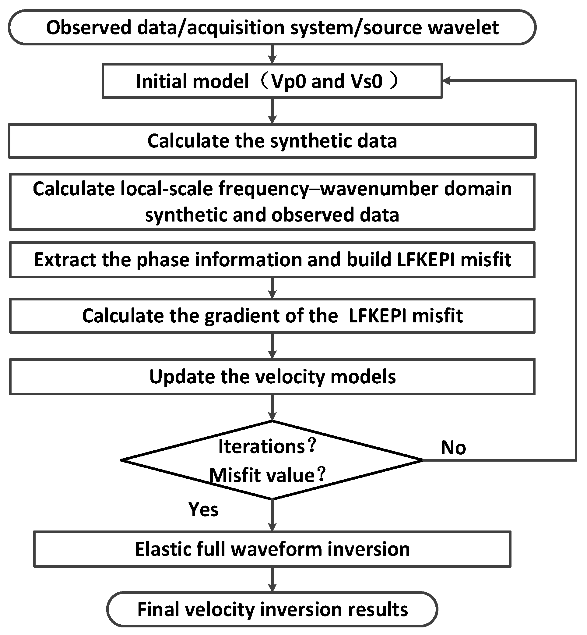
2.3. Elastic Wave Phase Inversion in the Local-Scale Frequency–Wavenumber Domain

To derive the local-scale frequency–wavenumber domain seismic data, this study utilizes a two-dimensional sliding Gaussian window function for the local-scale decomposition of the seismic data. This approach was integrated with a two-dimensional Fourier transform to extract the local scale frequency–wavenumber domain phases. The local scale forward and inverse transforms can be represented as follows [40]:

$$\left\{\begin{array}{l}\widehat{u}(\tau , h, \omega , k_x)=F_{2D}\left[u(t,x)\right]={\displaystyle \iint u(t,x) g(t-\tau ,x-h) e^{-i\left(\omega t-k_{x}x\right)}dt dx}\\ u(t,x)=F_{2D}^{*}\left[\widehat{u}(\tau , h, \omega , k_x)\right]={\displaystyle \iint {\displaystyle \iint \widehat{u}(\tau , h, \omega , k_x) g(t-\tau ,x-h)e^{i\left(\omega t-k_{x}x\right)} d\omega d{k}_x d\tau dh}}\end{array}\right.$$

(11)

where $F_{2D}\left[\cdot \right]$ and $F_{2D}^{*}\left[\cdot \right]$ denote the window-based two-dimensional Fourier forward and inverse transforms, respectively, $g(t,x)$ is the two-dimensional Gaussian window function with 0.18 s length and 0.6 km width, $k_x$ indicates the wavenumber in the distance direction, and $u(t,x)$ represents the original seismic data. The local scale frequency–wavenumber domain data obtained after decomposition and transformation will also be referred to as $\widehat{u}(\tau , h, \omega , k_x)$, where $\tau$ and $h$ are the displacements in the time and space dimensions, respectively.

In the local-scale frequency–wavenumber domain, we can conveniently obtain the amplitude and phase information of seismic data:

$$\left\{\begin{array}{l}\widehat{u}(\tau , h, \omega , k_x)=\left|\widehat{u}(\tau , h, \omega , k_x)\right| e^{i{\Phi }_u^{FK}}\\ \widehat{d}(\tau , h, \omega , k_x)=\left|\widehat{d}(\tau , h, \omega , k_x)\right| e^{i{\Phi }_d^{FK}}\end{array}\right.$$

(12)

where $\widehat{u}(\tau , h, \omega , k_x)$ and $\widehat{d}(\tau , h, \omega , k_x)$ represent the frequency–wavenumber domain synthetic and observed data, respectively. The inherent nonlinearity of the EFWI misfit often leads to inverted results that are prone to local minima. To address this issue, we propose an Elastic Wave Phase Inversion in local-scale frequency–wavenumber domain (LFKEPI), which aims to achieve improved initial velocity models for EFWI. The proposed LFKEPI misfit can be expressed as follows:

$$J(m)={\displaystyle \sum _{ns}{\displaystyle \underset{\tau ,h}{\iint } {\displaystyle \underset{\omega ,k_x}{\iint } {\left|e^{i{\Phi }_u^{FK}}-e^{i{\Phi }_d^{FK}}\right|}^2}}}\begin{array}{c}d\omega \end{array}d{k}_x\begin{array}{c}d\tau \end{array}dh$$

(13)

where ${\Phi }_u^{FK}$ and ${\Phi }_d^{FK}$ represent the phase components of the synthetic and observed data in the local scale frequency–wavenumber domain, respectively; the local-scale frequency–wavenumber domain exponential phase is $e^{i{\Phi }_u^{FK}}=\widehat{u}(\tau , h, \omega , k_x)/\left|\widehat{u}(\tau , h, \omega , k_x)\right|$, $e^{i{\Phi }_d^{FK}}=\widehat{d}(\tau , h, \omega , k_x)/\left|\widehat{d}(\tau , h, \omega , k_x)\right|$. The gradient of the LFKEPI misfit is as follows:

$${\displaystyle \frac{\partial J\left(m\right)}{\partial m}}={\displaystyle \sum _{ns}{\displaystyle \underset{\tau ,h}{\iint } {\displaystyle \underset{\omega ,k_x}{\iint } \mathrm{Re}\left[\left(e^{i{\Phi }_u^{FK}}-e^{i{\Phi }_d^{FK}}\right) \frac{\partial }{\partial m}\left(\frac{{\widehat{u}}^{ *}}{\left|\widehat{u}\right|}\right)\right]}}}\begin{array}{c}d\omega \end{array}d{k}_x\begin{array}{c}d\tau \end{array}dh$$

(14)

Applying the chain rule allows for further derivation with respect to the velocity parameter:

$${\displaystyle \frac{\partial J\left(m\right)}{\partial m}}={\displaystyle \sum _{ns}{\displaystyle \underset{\tau ,h}{\iint } {\displaystyle \underset{\omega ,k_x}{\iint } \mathrm{Re}\left\{ \left(\frac{\Delta \widehat{d}}{\left|\widehat{u}\right|}\frac{\partial {\widehat{u}}^{*}}{\partial m}-\frac{\Delta \widehat{d} {\widehat{u}}^{*}}{{\left|\widehat{u}\right|}^3}\mathrm{Re}\left[\widehat{u}\frac{\partial {\widehat{u}}^{*}}{\partial m}\right]\right)\right\}}}}\begin{array}{c}d\omega \end{array}d{k}_x\begin{array}{c}d\tau \end{array}dh$$

(15)

where $\Delta \widehat{d}=\left(e^{i{\Phi }_u^{FK}}-e^{i{\Phi }_d^{FK}}\right)$. After simplification, we can express the final partial derivative of the misfit concerning the velocity parameter as follows:

$${\displaystyle \frac{\begin{array}{c}\partial J(m)\end{array}}{\partial m}}={\displaystyle \sum _{ns}{\displaystyle \underset{t}{\int }\mathrm{Re} \left\{ F_{2D}^{*} \left\{\frac{\left[\Delta \widehat{d} {\left|\widehat{u}\right|}^2-\mathrm{Re}\left(\Delta \widehat{d} {\widehat{u}}^{*}\right) \widehat{u}\right]}{{\left|\widehat{u}\right|}^3} \right\} \right\}}} {\displaystyle \frac{\begin{array}{c}\partial u\end{array}}{\partial m}} dt$$

(16)

The corresponding adjoint source for the local-scale frequency–wavenumber domain phase inversion is given by the following:

$$f_s^{FK}=\mathrm{Re} \left\{ F_{2D}^{*} \left\{{\displaystyle \frac{\left[\Delta \widehat{d} {\left|\widehat{u}\right|}^2-\mathrm{Re}\left(\Delta \widehat{d} {\tilde{u}}^{*}\right) \widehat{u}\right]}{{\left|\widehat{u}\right|}^3+\beta }} \right\} \right\}$$

(17)

The adjoint sources for all receivers are back-propagated into the model space to correlate with the forward-propagated wavefield. This process enables the computation of the gradient for the LFKEPI method. In addition, considering the weights of seismic reflection wave signals against noise influence and avoiding the occurrence of zero in the denominator of the adjoint source, a threshold parameter $\beta ={10}^{-4}\max ⎣ {\left|\widehat{u}\right|}^3 ⎦$ is similarly defined. In Figure 1, we show an LFKEPI + EFWI flow chart.

To better understand the differences between EFWI, FEPI, and LFKEPI, this study presents a detailed comparison of the adjoint sources (Figure 2) derived from these three methods based on Equation (1) and the adjoint source formulation. The comparison demonstrates that the adjoint source obtained from FEPI is markedly affected by noise contamination. This issue arises because the product operation in the frequency domain corresponds to convolution in the time domain, which introduces considerable noise when transforming back to the time domain. In contrast, the local-scale frequency–wavenumber domain phase inversion employs a two-dimensional sliding Gaussian window function that effectively captures the local characteristics of the seismic data. This approach significantly suppresses the noise generated during the transformation process, thereby enhancing the stability and reliability of the inversion results.

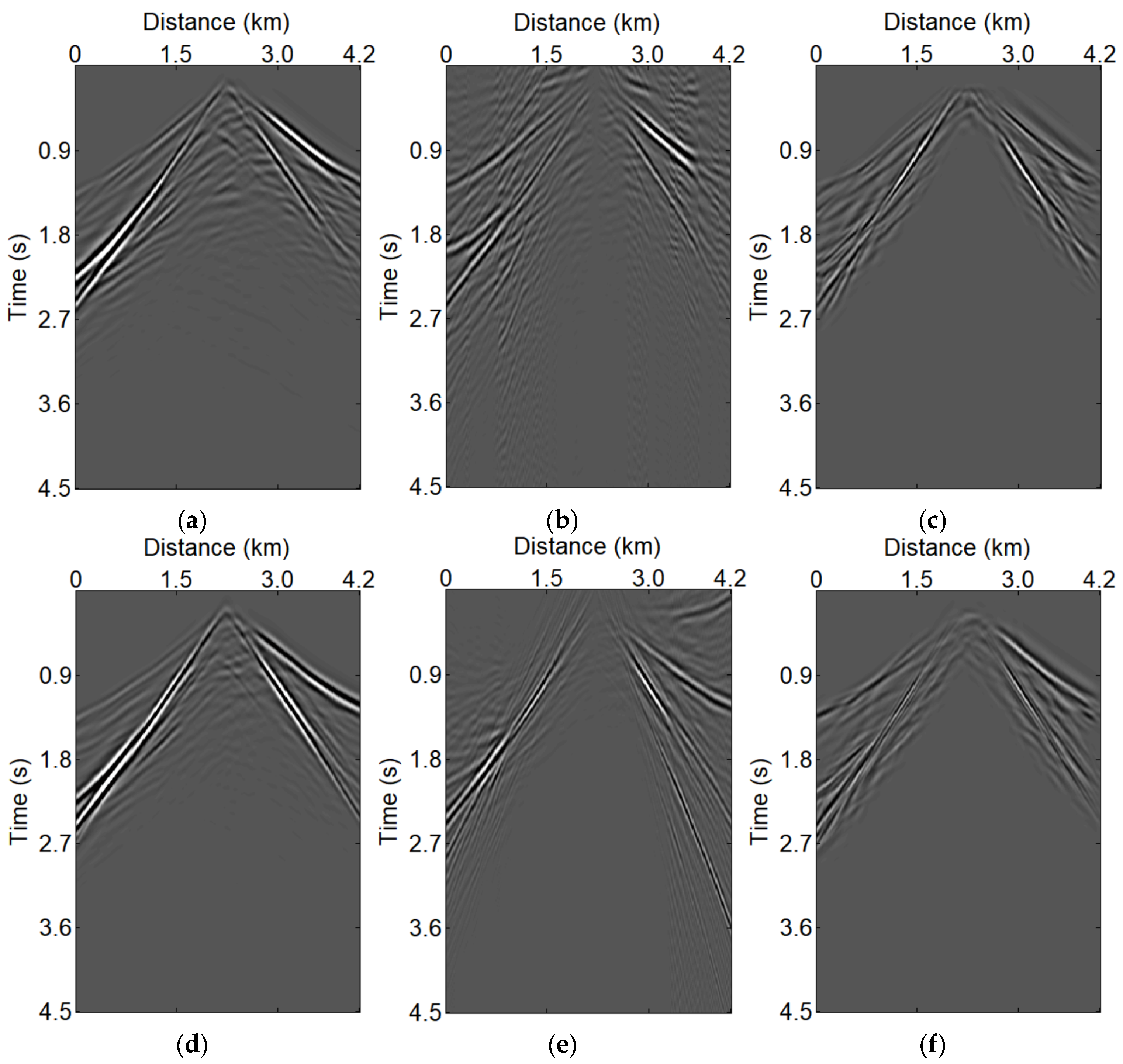
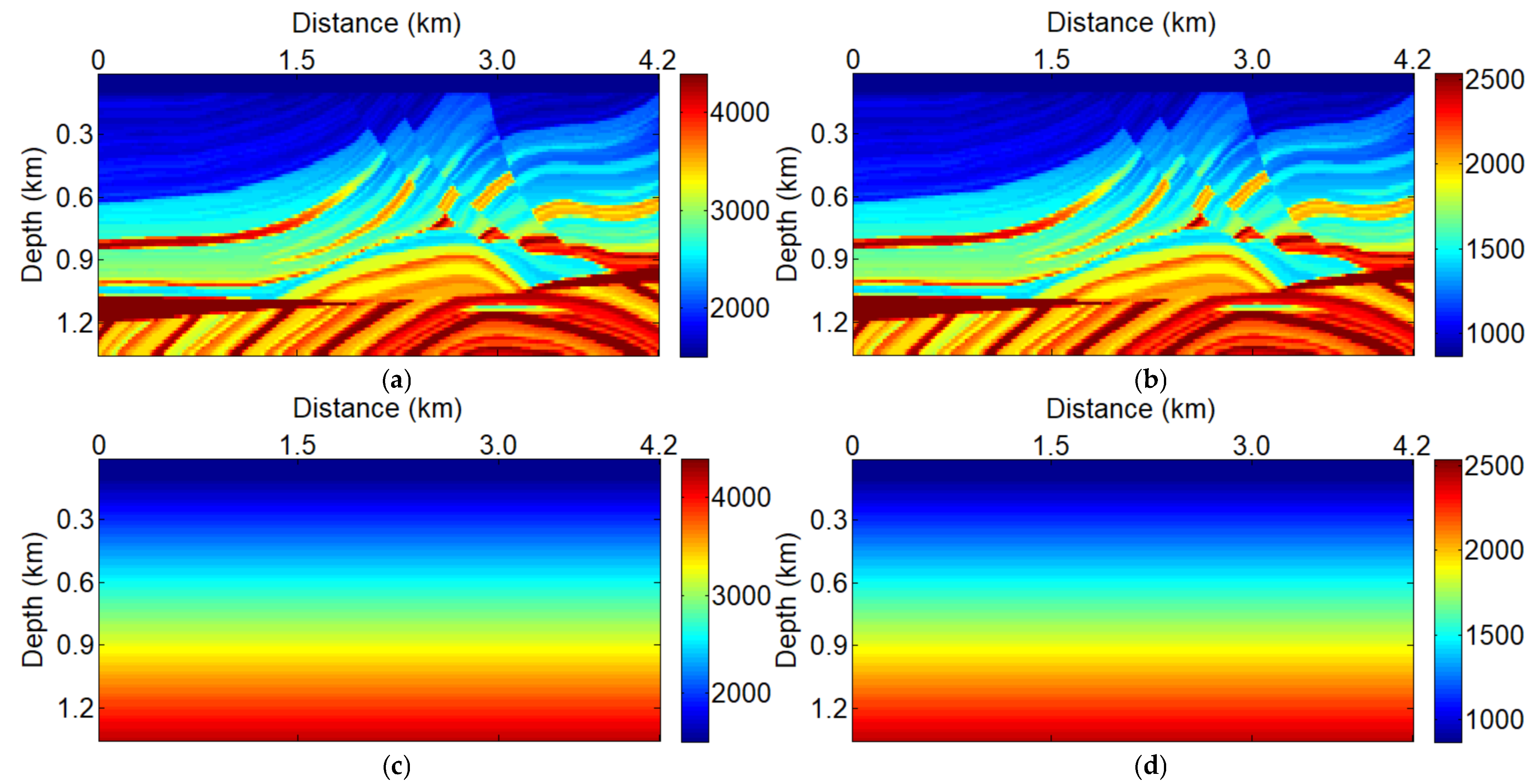
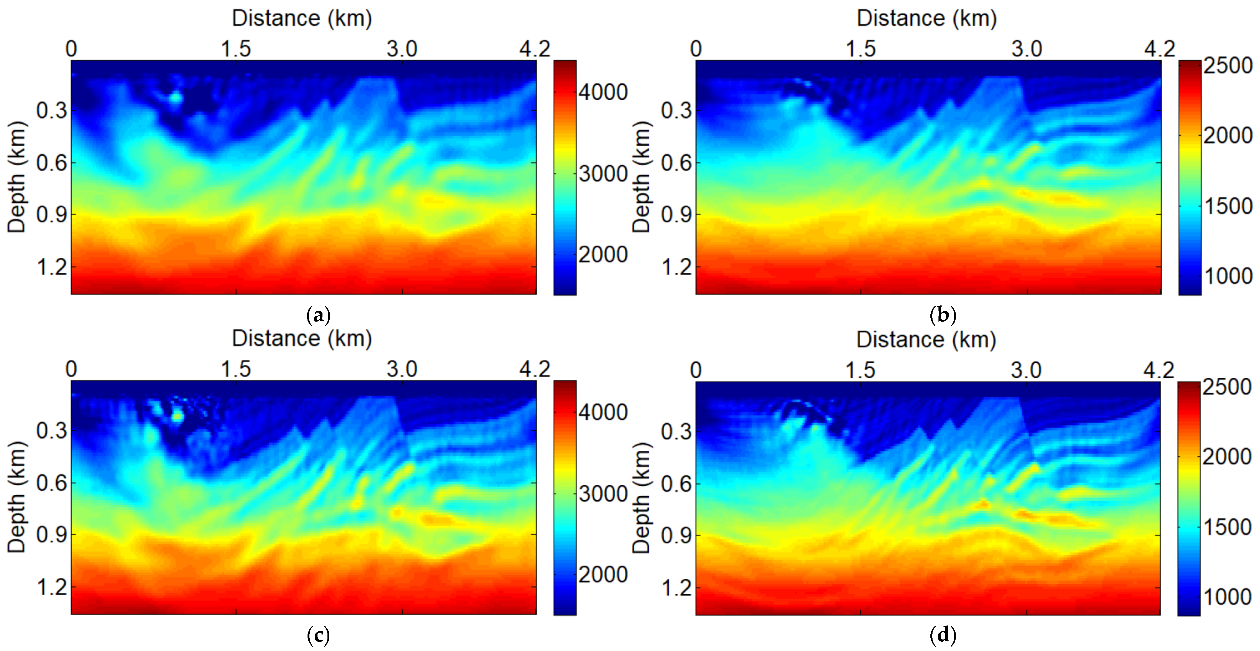
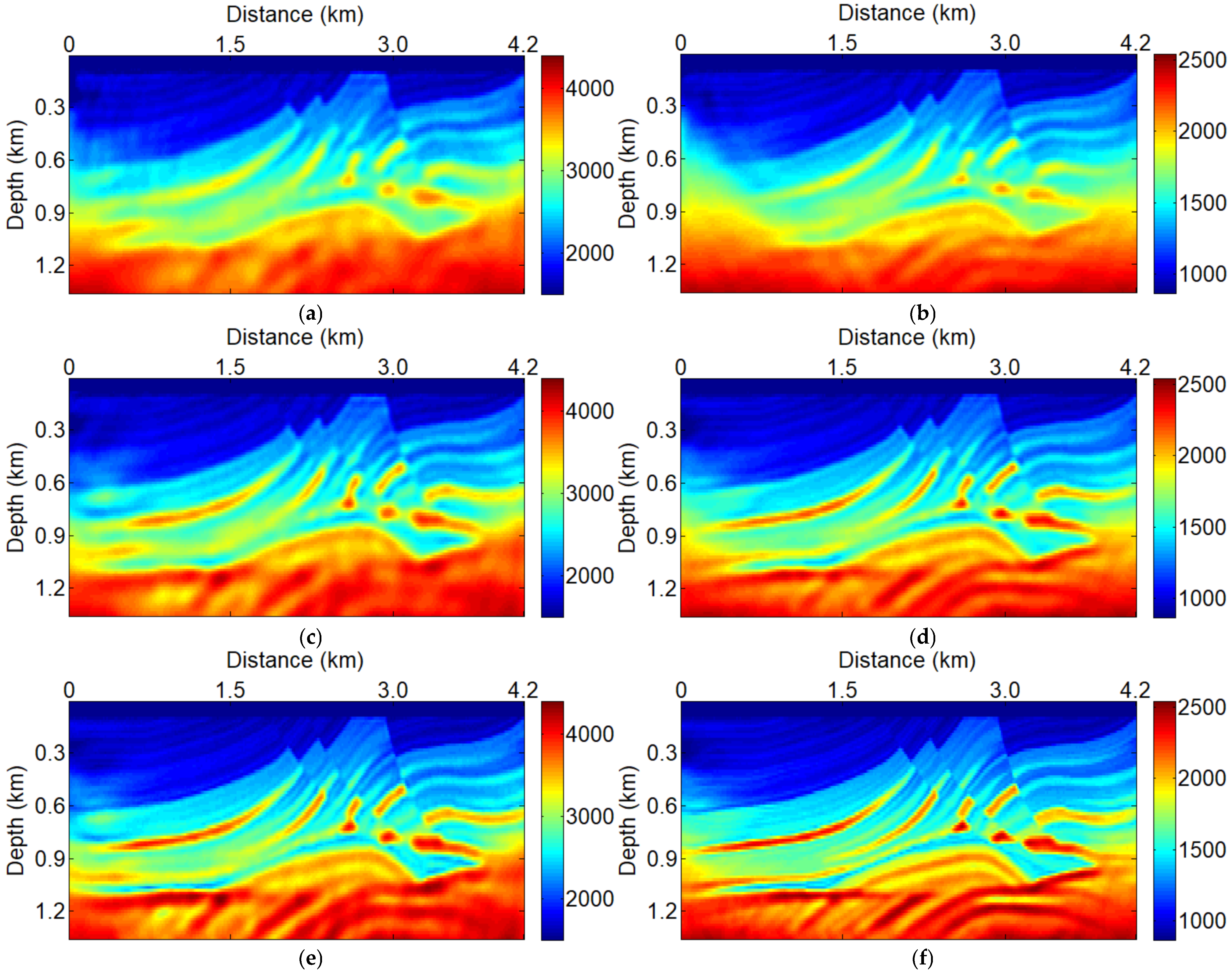
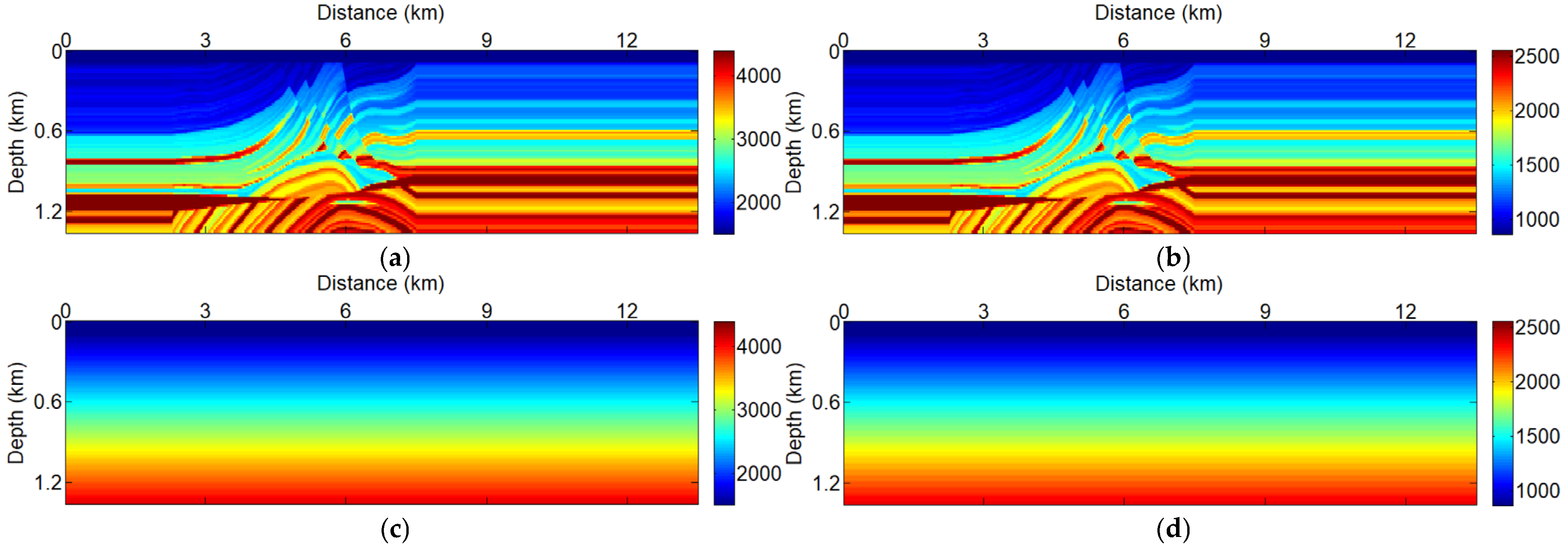
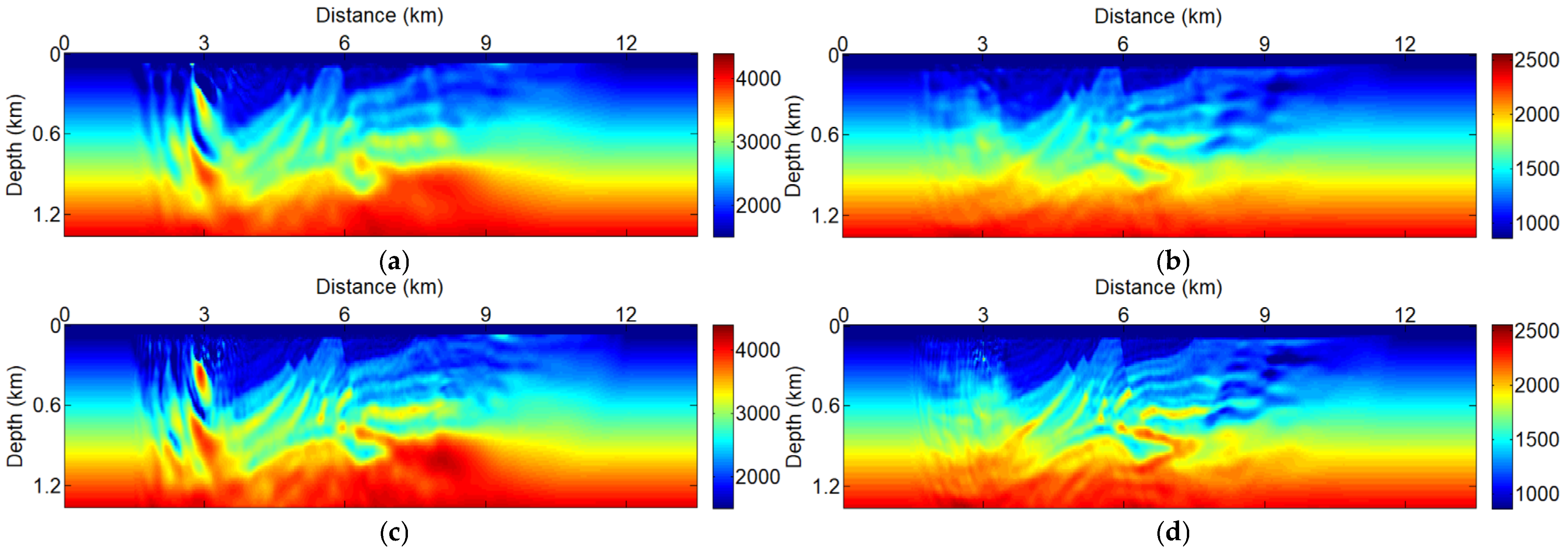
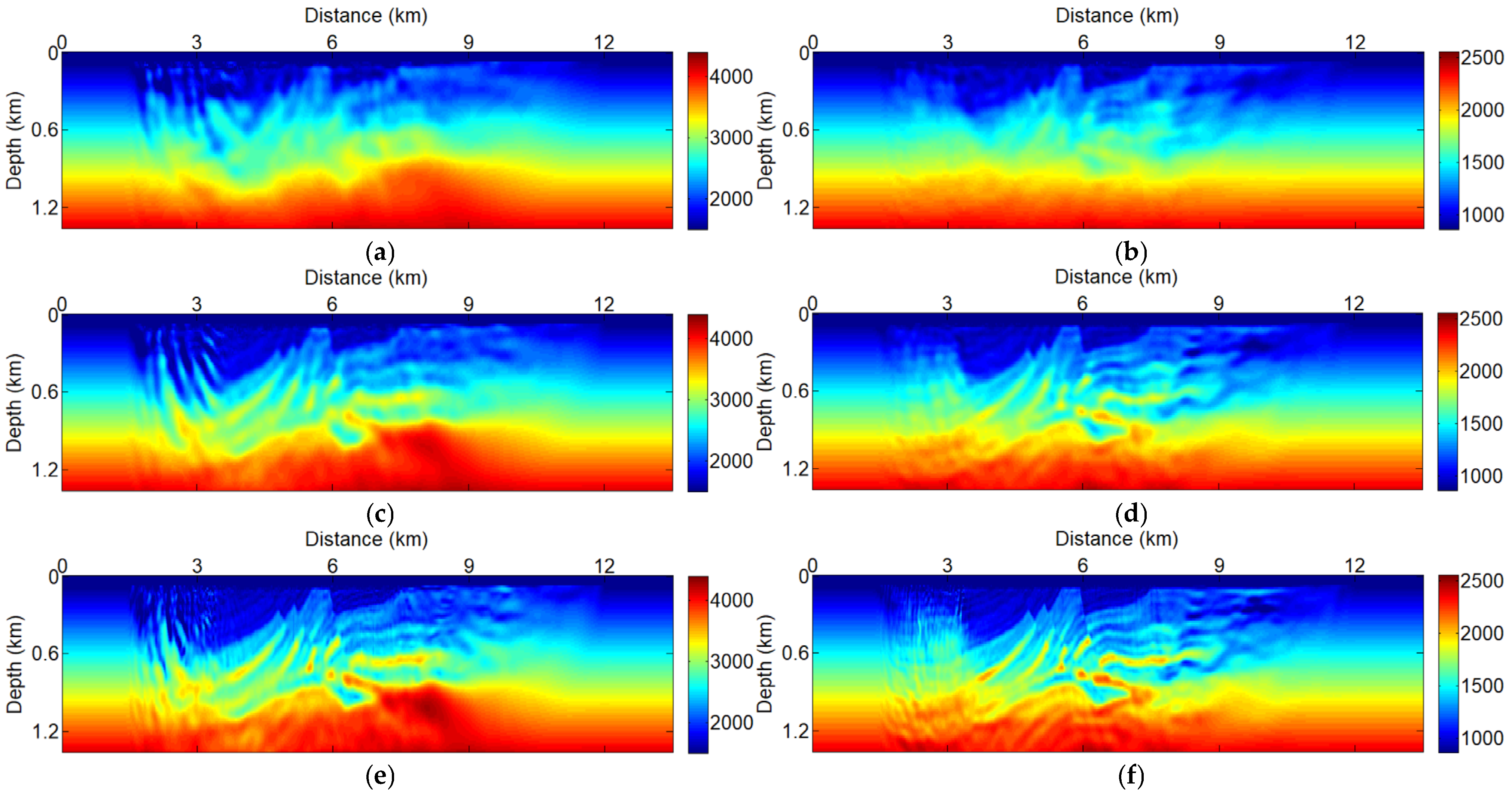
3. Numerical Testing

3.1. Land Seismic Acquisition System

To address the cycle-skipping of the EFWI method and to demonstrate the advantages of the LFKEPI approach for constructing macro-scale velocity models, numerical experiments were performed using the Marmousi model. Figure 3 displays both the true and the initial models used for inversion. The Marmousi model spans 4.2 km laterally and extends to a depth of 1.35 km. A total of 40 sources are evenly distributed along the surface, starting from 0.105 km with a spacing of 0.105 km between each source. The source wavelet employed is a Ricker wavelet with a peak frequency of 12 Hz. Seismic data were recorded for a duration of 4.5 s, sampled at 0.0018 s intervals.

The low-frequency components of seismic data reflect the large-scale structures. However, the seismic data often lack effective 0–4 Hz information, leading to cycle-skipping issues in EFWI. Therefore, during the testing process with the Marmousi models, we eliminate seismic data below 4 Hz. Firstly, we perform EFWI using only the 4–8 Hz low-frequency data, resulting in Figure 4a,b. Subsequently, Figure 4a,b are used as the initial velocity models for EFWI utilizing the 4–15 Hz high-frequency seismic data, yielding the result shown in Figure 4c,d. The multi-scale EFWI results for the Marmousi model exhibit significant discrepancies compared to the true velocity model, particularly in the left region of the model, where notable inversion errors occur. This is primarily attributed to the absence of 0–4 Hz information in the seismic data, causing the EFWI misfit to become trapped in a local minimum, thus preventing correct inversion results of the subsurface velocity models.

To alleviate the cycle-skipping issue in EFWI, we construct the misfit using the exponential phase information with frequency domain seismic data. Figure 5a,b present the results of the FEPI results. Compared to Figure 4a,b, the results show some improvements in the left region of the Marmousi model. However, compared to the true velocity models, a distinct abnormal velocity region still exists in the left area of the Marmousi models. Next, using Figure 5a,b as the initial models for EFWI, the inversion results displayed in Figure 4d and Figure 5c show improved resolution of the structural interfaces. Figure 5c,d are then used as the initial models for high-frequency band EFWI, resulting in Figure 5e,f. Despite these improvements, the abnormal velocity region remains uncorrected. This occurs because, when the low-wavenumber components of the velocity model are inaccurately inverted, using high-frequency data subsequently only clarifies interface inversion without correcting erroneous velocity values. A comparison between Figure 4 and Figure 5 reveals that, while the frequency domain phase inversion results demonstrate some improvements, the final inversion results still diverge significantly from the true velocity model, necessitating further enhancements.

To adequately consider the local features of seismic data in both time and offset directions, the seismic data are decomposed by a two-dimensional sliding Gaussian window function, combined with a two-dimensional Fourier transform to construct the phase misfit in the local scale frequency–wavenumber domain. The results of LFKEPI are shown in Figure 6a,b. A comparison of Figure 4, Figure 5 and Figure 6 reveals that the LFKEPI results for the Marmousi model are much closer to the true velocity model and do not exhibit any noticeable abnormal velocity regions. We then used Figure 6a,b as the initial velocity models for low-frequency band EFWI, and the inversion results are depicted in Figure 6c,d. Continuing with Figure 6c,d as the initial model for the high-frequency band EFWI, the final inversion results are presented in Figure 6e,f. It is evident that the inversion results in Figure 6c,d are the closest to the true velocity values of the Marmousi models.

A comparative analysis of the velocity profiles at a distance of 0.9 km from the Marmousi models is illustrated in Figure 7. The observed outcomes can be summarized as follows: (1) The EFWI results exhibit significant errors at shallow depths, primarily due to the absence of 0–4 Hz seismic data; (2) although the combination of FEPI and EFWI shows some improvements compared to the conventional EFWI results, significant disparities between the velocity values and the true values persist in the shallow regions, and the deeper areas fail to yield accurate velocity inversion results; (3) the LFKEPI + EFWI significantly enhances the shallow velocity inversion results while also effectively restoring the velocity values in the deeper regions.

Table 1. The model fit errors of EFWI, FEPI, and LFKEPI.

	EFWI	FEPI + EFWI	LFKEPI + EFWI
Vp	0.0168	0.024	0.0045
Vs	0.0188	0.0151	0.0048

presents the model fit errors of EFWI, FEPI, and LFKEPI, which are defined as follows:

$$\epsilon ={\displaystyle \frac{1}{N}}{{\displaystyle \sum _{i=1}^N\left[\frac{m_i^{true}-m_i^{inv}}{m_i^{true}}\right]}}^2$$

(18)

where $N$ is the total number of grids, $m_i^{true}$ denotes the true velocity at grid $i$, and $m_i^{inv}$ represents the inverted velocity at the same grid point. For Equation (18), a smaller model fit error indicates higher accuracy of the inversion result. Among the tested approaches in Table 1, the LFKEPI + EFWI yields the lowest model error. This further confirms that, even in the absence of low-frequency data, the LFKEPI + EFWI strategy can achieve high-resolution inversion results. Conversely, the FEPI + EFWI method produces larger Vp model errors compared to the EFWI results. The primary cause stems from the cycle-skipping problem at the left region of the Marmousi model, leading to significant localized errors that inflate the overall model fit error. Therefore, evaluating the performance of different inversion methods requires a comprehensive analysis that considers multiple metrics. Overall, the velocity inversion results, profile comparisons, and model fit error analysis on the Marmousi model demonstrate that the LFKEPI method offers a robust initial velocity model for EFWI, even when low-frequency seismic data below 4 Hz are missing. Therefore, the LFKEPI method can effectively mitigate the cycle-skipping problems commonly encountered during the EFWI process.

3.2. Marine Towed Seismic Acquisition Systems with Simultaneous Sources

Building on the previous numerical experiments, we performed additional tests using a marine towed simultaneous sources-based seismic acquisition system, as illustrated in Figure 8. The survey line consists of 400 shot gathers with uniform shot and receiver intervals of 15 m, resulting in a maximum offset of 4.65 km. The first source is located at 1.5 km, while the 400th source is positioned at 7.485 km. To improve computational efficiency in velocity modeling, 20 consecutive sources were combined into a single simultaneous source (Figure 8), with phase encoding applied to suppress crosstalk noise between simultaneous sources. Due to the inherent acquisition characteristic where the receiver array shifts forward by one position after each shot, data from these 20 adjacent shots can be combined into a new simultaneous source dataset. However, only receiver channels common to all 20 shots were retained, necessitating the exclusion of data at both streamer ends. Consequently, the effective streamer length for simultaneous source data is reduced to 4.35 km. Despite the data volume reduction, this grouping approach achieves a twentyfold increase in computational efficiency, confirming the feasibility of the marine towed simultaneous source-based seismic acquisition system strategy.

Using the modified Marmousi models (Figure 9a,b) and linear initial velocity models (Figure 9c,d), we evaluated three inversion algorithms: (1) Simultaneous Source-based Elastic Full Waveform Inversion (SS-EFWI); (2) Simultaneous Source-based Elastic Wave Phase Inversion in the Frequency Domain (SS-FEPI); and (3) Simultaneous Source-based Elastic Wave Phase Inversion in the local-scale frequency–wavenumber domain (SS-LFKEPI). The modified Marmousi models span 13.5 km horizontally and 1.35 km vertically, discretized with a grid spacing of 15 m. A total of 400 shot gathers were simulated, with source locations distributed between 1.5 km and 7.5 km within the model. The source wavelet has a central frequency of 8 Hz, the maximum recording time is 5.4 s, and the temporal sampling interval is 1.8 ms. To test the robustness of the SS-LFKEPI method against cycle skipping, frequencies below 4 Hz were removed using a low-frequency filter during the numerical experiments.

To investigate the cycle skipping of SS-EFWI, we filtered out 0–4Hz seismic data during tests with the Marmousi models. First, EFWI was performed using marine towed simultaneous sources and only the low-frequency band (4–8 Hz), producing the velocity models shown in Figure 10a,b. These models then served as initial velocity fields for a subsequent SS-EFWI using the high-frequency band (4–15 Hz) seismic data, resulting in the velocity updates shown in Figure 10c,d. Despite this multiscale SS-EFWI approach, the inversion results still fail to accurately recover the complex geological structures of the Marmousi models. This limitation is primarily due to the absence of 0–4 Hz seismic data, which causes the SS-EFWI misfit to be trapped in local minima and prevents the recovery of high-resolution subsurface velocity structures. Thus, it is essential to develop improved methods that effectively address the cycle-skipping issue inherent to the SS-EFWI method.

We applied the SS-FEPI method to invert elastic seismic data lacking low-frequency components, as shown in Figure 10b and Figure 11a. These results served as initial models for low-frequency band SS-EFWI, which improved the resolution of structural interfaces (Figure 10d and Figure 11c). Subsequently, Figure 11c,d were used as starting models for high-frequency band SS-EFWI, yielding the final velocity models in Figure 11e,f. Although the phase information exhibits a better linear relationship with subsurface structures, a velocity anomaly remains unresolved. This limitation arises from inaccuracies in the inversion of low-wavenumber velocity components; thus, subsequent high-frequency inversion enhances interface sharpness but fails to correct erroneous velocity values. The comparison of results in Figure 10 and Figure 11 shows that, while the SS-FEPI + SS-EFWI scheme yields improvements, the final inversion still significantly deviates from the true velocity model, underscoring the need for further methodological developments.

To further validate the advantages of the SS-LFKEPI method in reconstructing the low-wavenumber information of velocity models and to improve its computational efficiency, we implemented a marine towed simultaneous source-based seismic acquisition system in the numerical experiments. The SS-LFKEPI results are presented in Figure 12a,b. These models were then used as the initial velocity models for low-frequency data SS-EFWI, yielding the inversion results shown in Figure 12c,d. Subsequently, Figure 12c,d served as initial models for high-frequency band SS-EFWI, producing the final velocity models depicted in Figure 12e,f. It is clear that the velocity models in Figure 12c,d most closely approximate the true Marmousi velocity fields. Comparing Figure 10, Figure 11 and Figure 12, the SS-LFKEPI approach consistently delivers velocity models that are significantly closer to the true Marmousi model. Among the tested methods in

Table 2. The model fit errors of SS-EFWI, SS-FEPI, and SS-LFKEPI.

	SS-EFWI	SS-FEPI + SS-EFWI	SS-LFKEPI + SS-EFWI
Vp	0.0191	0.0151	0.0143
Vs	0.0182	0.0179	0.0173

, the SS-LFKEPI + SS-EFWI yields the lowest model error. This further confirms that, even in the absence of low-frequency data, the SS-LFKEPI+ SS-EFWI strategy can achieve high-resolution inversion results. These findings further confirm that the combined SS-LFKEPI and SS-EFWI methodology offers substantial advantages for the high-resolution inversion of elastic parameter velocity fields in complex geological structures.

4. Conclusions

This paper presents an Elastic Wave Phase Inversion in local-scale frequency–wavenumber domain (LFKEPI) that integrates strategies for the two-dimensional local-scale decomposition of elastic seismic data and two-dimensional Fourier transforms. This approach adequately accounts for the local-scale characteristics of elastic seismic data to mitigate the cycle-skipping problem inherent in elastic full waveform inversion (EFWI). By constructing an exponential phase misfit in the local-scale frequency–wavenumber domain, it aids in recovering low-wavenumber information of the velocity parameters, allowing for a clearer interpretation of the subsurface structure, which can subsequently be refined using EFWI for improved accuracy in velocity inversion. Testing results from the Marmousi model with marine towed simultaneous sources indicates that the LFKEPI method can provide favorable initial velocity models for EFWI, alleviating the cycle skipping and ultimately yielding high-resolution velocity inversion results.

References

1. Lailly, P.; Bednar, J. The seismic inverse problem as a sequence of before stack migrations. In Conference on Inverse Scattering: Theory and Application; SIAM: Philadelphia, PA, USA, 1983; pp. 206–220. [Google Scholar]
2. Tarantola, A. Inversion of seismic reflection data in the acoustic approximation. Geophysics 1984, 49, 1259–1266. [Google Scholar] [CrossRef]
3. Tarantola, A. A strategy for nonlinear elastic inversion of seismic reflection data. Geophysics 1986, 51, 1893–1903. [Google Scholar] [CrossRef]
4. Plessix, R.-E. A review of the adjoint-state method for computing the gradient of a functional with geophysical applications. Geophys. J. Int. 2006, 167, 495–503. [Google Scholar] [CrossRef]
5. Virieux, J.; Operto, S. An overview of full-waveform inversion in exploration geophysics. Geophysics 2009, 74, WCC1–WCC26. [Google Scholar] [CrossRef]
6. Wu, R.-S.; Luo, J.; Wu, B. Seismic envelope inversion and modulation signal model. Geophysics 2014, 79, Wa13–Wa24. [Google Scholar] [CrossRef]
7. Alkhalifah, T. Full-model wavenumber inversion: An emphasis on the appropriate wavenumber continuation. Geophysics 2016, 81, R89–R98. [Google Scholar] [CrossRef]
8. Alkhalifah, T.; Choi, Y. From tomography to full-waveform inversion with a single objective function. Geophysics 2014, 79, R55–R61. [Google Scholar] [CrossRef]
9. Wang, Y.; Rao, Y. Crosshole seismic waveform tomography–I. Strategy for real data application. Geophys. J. Int. 2006, 166, 1224–1236. [Google Scholar] [CrossRef]
10. Crase, E.; Wideman, C.; Noble, M.; Tarantola, A. Nonlinear elastic waveform inversion of land seismic reflection data. J. Geophys. Res. Solid Earth 1992, 97, 4685–4703. [Google Scholar] [CrossRef]
11. Liu, Y.; Huang, X.; Wan, X.; Sun, M.; Dong, L. Elastic multi-parameter full-waveform inversion for anisotropic media. Chin. J. Geophys. 2019, 62, 1809–1823. (In Chinese) [Google Scholar]
12. Bunks, C.; Saleck, F.M.; Zaleski, S.; Chavent, G. Multiscale seismic waveform inversion. Geophysics 1995, 60, 1457–1473. [Google Scholar] [CrossRef]
13. Pratt, R.G.; Shin, C.; Hicks, G.J. Gauss-Newton and full Newton methods in frequency-space seismic waveform inversion. Geophys. J. Int. 1998, 133, 341–362. [Google Scholar] [CrossRef]
14. Guo, X.B.; Liu, H.; Shi, Y. Time domain full waveform inversion based on frequency attenuation. Chin. J. Geophys. 2016, 59, 3777–3787. (In Chinese) [Google Scholar]
15. Chen, S.C.; Chen, G.X. Time-damping full waveform inversion of multi-dominant-frequency wavefields. Chin. J. Geophys. 2017, 60, 3229–3237. (In Chinese) [Google Scholar] [CrossRef]
16. Shin, C.; Ho Cha, Y. Waveform inversion in the Laplace-Fourier domain. Geophys. J. Int. 2009, 177, 1067–1079. [Google Scholar] [CrossRef]
17. Kwon, J.; Jun, H.; Song, H.; Jang, U.G.; Shin, C. Waveform inversion in the shifted Laplace domain. Geophys. J. Int. 2017, 210, 340–353. [Google Scholar] [CrossRef]
18. Ha, W.; Shin, C. Deconvolution-Based Objective Functions for Full Waveform Inversion in the Laplace Domain. IEEE Trans. Geosci. Remote Sens. 2022, 60, 5904708. [Google Scholar] [CrossRef]
19. Chi, B.X.; Dong, L.G.; Liu, Y.Z. Full waveform inversion method using envelope objective function without low frequency dataJ. J. Appl. Geophys. 2014, 109, 36–46. [Google Scholar] [CrossRef]
20. Zhang, P.; Wu, R.S.; Han, L. Seismic Envelope Inversion Based on Hybrid Scale Separation for Data with Strong Noises. Pure Appl. Geophys. 2019, 176, 165–188. [Google Scholar] [CrossRef]
21. Hu, Y.; Wu, R.S.; Han, L.G.; Zhang, P. Joint Multiscale Direct Envelope Inversion of Phase and Amplitude in the Time–Frequency Domain. IEEE Trans. Geosci. Remote Sens. 2019, 57, 5108–5120. [Google Scholar] [CrossRef]
22. Zhang, P.; Han, L.; Zhang, F.; Feng, Q.; Chen, X. Wavefield Decomposition-Based Direct Envelope Inversion and Structure-Guided Perturbation Decomposition for Salt Building. Minerals 2021, 11, 919. [Google Scholar] [CrossRef]
23. Chen, G.; Yang, W.; Liu, Y.; Luo, J.; Jing, H. Envelope-Based Sparse-Constrained Deconvolution for Velocity Model Building. IEEE Trans. Geosci. Remote Sens. 2022, 60, 4501413. [Google Scholar] [CrossRef]
24. Wang, Y.; Chi, B.; Dong, L. Envelope normalized reflection waveform inversion. Geophys. Prospect. 2024, 73, 895–909. [Google Scholar] [CrossRef]
25. Xiong, K.; Lumley, D.; Zhou, W. Improved seismic envelope full-waveform inversion. Geophysics 2023, 88, R421–R437. [Google Scholar] [CrossRef]
26. Hu, Y.; Wu, R.S.; Huang, X.; Long, Y.; Xu, Y.; Han, L.G. Phase-amplitude-based polarized direct envelope inversion in the time-frequency domain. Geophysics 2022, 87, R245–R260. [Google Scholar] [CrossRef]
27. Sirgue, L.; Pratt, R.G. Efficient waveform inversion and imaging: A strategy for selecting temporal frequencies. Geophysics 2004, 69, 231–248. [Google Scholar] [CrossRef]
28. Luo, J.; Wu, R.-S.; Gao, F. Time-domain full waveform inversion using instantaneous phase information with damping. J. Geophys. Eng. 2018, 15, 1032. [Google Scholar] [CrossRef]
29. Bednar, J.B.; Shin, C.; Pyun, S. Comparison of waveform inversion, part 2: Phase approach. Geophys. Prospect. 2007, 55, 465–475. [Google Scholar] [CrossRef]
30. Sun, Y. Time-domain phase inversion. SEG Tech. Program Expand. Abstr. 1993, 12, 1396. [Google Scholar]
31. Fu, L.; Guo, B.; Schuster, G.T. Multiscale phase inversion of seismic data. Geophysics 2017, 83, R159–R171. [Google Scholar] [CrossRef]
32. Choi, Y. Time-domain pure-phase inversion of wavefield in exponential damping. J. Appl. Geophys. 2022, 204, 104734. [Google Scholar] [CrossRef]
33. Fichtner, A.; Kennett, B.L.N.; Igel, H.; Bunge, H.-P. Theoretical background for continental-and global-scale full-waveform inversion in the time–frequency domain. Geophys. J. Int. 2008, 175, 665–685. [Google Scholar] [CrossRef]
34. Hu, Y.; Han, L.; Wu, R.; Xu, Y. Multi-scale time-frequency domain full waveform inversion with a weighted local correlation-phase misfit function. J. Geophys. Eng. 2019, 16, 1017–1031. [Google Scholar] [CrossRef]
35. Kang, P.; Hu, Y.; Liu, R.; Sun, C.; Zhao, Z.; Yuan, P.; Zhen, M.; Meng, Y.; Xu, Y. Local-scale frequency-wavenumber domain phase inversion. Prog. Geophys. 2025, 40, 155–165. [Google Scholar]
36. Zhu, H.; Fomel, S. Building good starting models for full-waveform inversion using adaptive matching filtering misfit. Geophysics 2016, 81, U61–U72. [Google Scholar] [CrossRef]
37. Warner, M.; Guasch, L. Adaptive waveform inversion. Theory J. Geophys. 2016, 81, R429–R445. [Google Scholar] [CrossRef]
38. Hu, Y.; Han, L.; Zhang, P.; Ge, Q. Time-frequency domain multi-scale full waveform inversion based on adaptive non-stationary phase correction. Chin. J. Geophys. 2018, 61, 2969–2988. (In Chinese) [Google Scholar]
39. Tao, L.; Gu, Z.; Ren, H. Improving the Seismic Impedance Inversion by Fully Convolutional Neural Network. J. Mar. Sci. Eng. 2025, 13, 262. [Google Scholar] [CrossRef]
40. Hu, Y.; Fu, L.-Y.; Li, Q.; Deng, W.; Han, L. Frequency-Wavenumber Domain Elastic Full Waveform Inversion with a Multistage Phase Correction. Remote Sens. 2022, 14, 5916. [Google Scholar] [CrossRef]
Figure 1. The flowchart of the LFKEPI + EFWI method.
Jmse 13 00964 g001
Figure 2. Horizontal displacement adjoint sources of the (a) EFWI, (b) FEPI, (c) LFKEPI; vertical displacement adjoint sources of the (d) EFWI, (e) FEPI, (f) LFKEPI.
Jmse 13 00964 g002
Figure 3. Marmousi velocity models: (a) True Vp. (b) True Vs. (c) Initial Vp. (d) Initial Vs.
Jmse 13 00964 g003
Figure 4. Results of multi-scale EFWI: (a) Vp model EFWI result with a low-frequency band (4–8 Hz); (b) Vs model EFWI result with a low-frequency band (4–8 Hz); (c) Vp model EFWI result with a low-frequency band (4–15 Hz), using (a) as the initial model; (d) Vs model EFWI result with a low-frequency band (4–15 Hz), using (b) as the initial model.
Jmse 13 00964 g004
Figure 5. Results of FEPI + EFWI: (a) Vp model FEPI result with a low-frequency band (4–8 Hz); (b) Vs model FEPI result with a low-frequency band (4–8 Hz); (c) Vp model FEPI + EFWI result with a low-frequency band (4–8 Hz), using (a) as the initial model; (d) Vs model FEPI + EFWI result with a low-frequency band (4–8 Hz), using (b) as the initial model; (e) Vp model FEPI + EFWI result with a low-frequency band (4–15 Hz), using (c) as the initial model; (f) Vs model FEPI + EFWI result with a low-frequency band (4–15 Hz), using (d) as the initial model.
Jmse 13 00964 g005
Figure 6. Results of LFKEPI + EFWI: (a) Vp model LFKEPI result with a low-frequency band (4–8 Hz); (b) Vs model LFKEPI result with a low-frequency band (4–8 Hz); (c) Vp model LFKEPI + EFWI result with a low-frequency band (4–8 Hz), using (a) as the initial model; (d) Vs model LFKEPI + EFWI result with a low-frequency band (4–8 Hz), using (b) as the initial model; (e) Vp model LFKEPI + EFWI result with a low-frequency band (4–15 Hz), using (c) as the initial model; (f) Vs model LFKEPI + EFWI result with a low-frequency band (4–15 Hz), using (d) as the initial model.
Jmse 13 00964 g006
Figure 7. Comparison of velocity inversion profiles located at 0.9 km from the Marmousi models of Vp and Vs: (a) Vp model of EFWI result; (b) Vp model of FEPI + EFWI result; (c) Vp model of LFKEPI + EFWI result; (d) Vs model of EFWI result; (e) Vs model of FEPI + EFWI result; (f) Vs model of LFKEPI + EFWI result.
Jmse 13 00964 g007
Figure 8. A marine towed simultaneous sources-based seismic acquisition system.
Jmse 13 00964 g008
Figure 9. Modified Marmousi velocity models: (a) True Vp. (b) True Vs. (c) Initial Vp. (d) Initial Vs.
Jmse 13 00964 g009
Figure 10. Results of multi-scale SS-EFWI: (a) Vp model SS-EFWI result with a low-frequency band (4–8 Hz); (b) Vs model SS-EFWI result with a low-frequency band (4–8 Hz); (c) Vp model SS-EFWI result with a low-frequency band (4–15 Hz), using (a) as the initial model; (d) Vs model SS-EFWI result with a low-frequency band (4–15 Hz), using (b) as the initial model.
Jmse 13 00964 g010
Figure 11. Results of SS-FEPI + SS-EFWI: (a) Vp model SS-FEPI result with a low-frequency band (4–8 Hz); (b) Vs model SS-FEPI result with a low-frequency band (4–8 Hz); (c) Vp model SS-FEPI + SS-EFWI result with a low-frequency band (4–8 Hz), using (a) as the initial model; (d) Vs model SS-FEPI + SS-EFWI result with a low-frequency band (4–8 Hz), using (b) as the initial model; (e) Vp model SS-FEPI + SS-EFWI result with a low-frequency band (4–15 Hz), using (c) as the initial model; (f) Vs model SS-FEPI + SS-EFWI result with a low-frequency band (4–15 Hz), using (d) as the initial model.
Jmse 13 00964 g011
Figure 12. Results of SS-LFKEPI + SS-EFWI: (a) Vp model SS-LFKEPI result with a low-frequency band (4–8 Hz); (b) Vs model SS-LFKEPI result with a low-frequency band (4–8 Hz); (c) Vp model SS-LFKEPI + SS-EFWI result with a low-frequency band (4–8 Hz), using (a) as the initial model; (d) Vs model SS-LFKEPI + SS-EFWI result with a low-frequency band (4–8 Hz), using (b) as the initial model; (e) Vp model SS-LFKEPI + SS-EFWI result with a low-frequency band (4–15 Hz), using (c) as the initial model; (f) Vs model SS-LFKEPI + SS-EFWI result with a low-frequency band (4–15 Hz), using (d) as the initial model.
Jmse 13 00964 g012