Abstract
In marine seismic surveys, towed streamers record only pressure data with limited offsets and insufficient low-frequency content, whereas Ocean Bottom Nodes (OBNs) acquire multi-component data with wider offset and sufficient low-frequency content, albeit with sparser spatial sampling. Elastic full waveform inversion (EFWI) is used to estimate subsurface elastic properties by matching observed and synthetic data. However, using only towed streamer data makes it impossible to reliably estimate shear-wave velocities due to the absence of direct S-wave recordings and limited illumination. Inversion using OBN data is prone to acquisition footprint artifacts. To overcome these challenges, we propose a hierarchical joint inversion method based on P- and S-wave separation (PS-JFWI). We first derive novel acoustic-elastic coupled equations based on wavefield separation. Then, we design a two-stage inversion framework. In Stage I, we use OBN data to jointly update the P- and S-wave velocity models. In Stage II, we apply a gradient decoupling algorithm: we construct the P-wave velocity gradient by combining the gradient using PP-waves from both towed streamer and OBN data and construct the S-wave velocity gradient using the gradient using PS-waves. Numerical experiments demonstrate that the proposed method enhances the inversion accuracy of both velocity models compared with single-source and conventional joint inversion methods.
1. Introduction
Full waveform inversion (FWI) has emerged as a powerful high-resolution subsurface imaging technique. For decades, FWI algorithms based on the adjoint-state method have provided the foundational methodology for inverting subsurface parameters such as impedance, velocity, density, and quality factor from pre-stack seismic data [1,2,3,4]. Since the establishment of its theoretical framework, FWI has evolved from acoustic to elastic medium approximation to recover the elastic properties of the subsurface [5,6]. Acoustic FWI (AFWI) is commonly used to reconstruct the P-wave velocity model, but it becomes less effective when long-wavelength variations in the S-wave velocity are present [7,8,9]. With advancements in high-performance computing, elastic FWI (EFWI) has shown significant potential for simultaneously inverting P-wave velocity (), S-wave velocity (), and density [10,11]. However, in multi-parameter inversion, strong coupling in the nonlinear problem and differences in parameter sensitivities can lead the inversion to become trapped in local minima [12,13,14]. Through analysis of radiation characteristics in PP (P-wave reflected as P-wave), PS (P-wave converted to S-wave), SP (S-wave converted to P-wave), and SS (S-wave reflected as S-wave) scattering patterns, Forgues and Lambaré [15] demonstrated that crosstalk between and remains non-negligible for PP-wave modes at moderate scattering angles. Tarantola’s research corroborated that even in models with constant , perturbations in significantly modulate the PP-wave diffraction [16]. To enhance the accuracy of P- and S-wave velocity inversion, Wang & Cheng [17] and Ren & Liu [18] proposed an innovative strategy: incorporating wavefield mode decoupling and a hierarchical inversion framework into EFWI. The multi-parameter crosstalk can be suppressed by employing the decoupled gradients.
In marine seismic exploration, towed streamer data are widely used due to their low cost, high acquisition efficiency, and high horizontal resolution. FWI using towed streamer data has achieved many reasonable examples [19,20,21]. However, the inherent characteristics of towed streamer acquisition limit its effectiveness in EFWI. Although the development of acoustic-elastic coupled equations (AECE) makes it possible to apply EFWI to towed streamer data [22], the data usually have limited offsets, lack low-frequency content, and contain only pressure components due to the limitations of hydrophone deployment and recording [23,24,25]. Considering that FWI is a nonlinear local optimization problem, these limitations make it difficult to estimate the S-wave velocity and increase the risk of falling into local minima [26,27].
In contrast, OBNs record multi-component seismic data with wide azimuth coverage and low-frequency information [28]. The availability of vertical and horizontal components significantly enhances sensitivity to S-waves, making OBN data particularly suitable for estimating model [29]. Furthermore, their wide-angle wavefields are beneficial for building large-scale background velocity models. However, the sparse spatial distribution [30] of seismic sensors creates difficulties for conventional EFWI in suppressing acquisition footprints [31]. Notably, the wavefield propagation paths of towed streamer and OBN data are highly complementary: OBNs offer wide-angle coverage and can record full wavefields, which are beneficial for building the macro-scale velocity model [32], while densely sampled towed streamer data provide high-resolution constraints in the shallow subsurface due to their short offset range and high spatial sampling density [33,34]. Joint inversion strategies have received increasing attention in recent years [35,36,37]. Many existing methods use simple gradient weighting, such as by offset range, inversion depth, or iteration number. These approaches help balance different data types, but parameter decoupling and optimization in multi-wavefield inversion are still ongoing research topics.
To address these challenges, we develop a hierarchical joint FWI approach based on P- and S-wave separation (PS-JFWI). In this study, we first systematically introduce the theoretical framework of AECE and derive the formulations of P- and S-wave separation. We propose the hierarchical inversion algorithm and gradient decoupling strategies. The inversion proceeds in two stages: In Stage I, we implement traditional EFWI using only OBN data to obtain initial estimates of P- and S-wave velocities. In Stage II, to mitigate the coupling between velocity parameters, we compute the gradient for using separated forward and adjoint P-wavefields (i.e., the gradient using PP-wave) and the gradient for using forward P-wave and adjoint S-wavefields (i.e., the gradient using PS-wave). Then, we use a simple anomaly model and the overthrust model to test our proposed method. Finally, we have a discussion and a conclusion.
2. Methodology
In this section, we derive the acoustic-elastic coupled equations (AECE) based on P- and S-wave separation and the corresponding gradient equations. Based on this, we describe the joint inversion strategy in detail.
2.1. Acoustic-Elastic Coupled Equations Based on P- and S-Wave Separation
The first-order velocity-stress elastic wave equation can be given as follows:
where and denote horizontal and vertical particle velocity components, respectively; , , and are stress components; and are Lamé parameters; is density; t is the forward moment; and x and z are the horizontal and vertical positions in the model, respectively.
To describe wave propagation in an acoustic-elastic coupled medium, the wave equation [Equation (1)] is reformulated via partial stress decomposition, leading to the AECE [22]:
where , , and are deviatoric stress components, while represents the acoustic pressure component. This formulation inherently isolates pure P-waves by decoupling pressure and shear stress contributions. The relationship between the stress components , , and in Equation (1) and the deviatoric stress components , , , and in Equation (2) satisfy the following formulas:
To achieve P- and S-wavefield separation, the stress components are decomposed into a P-wave stress component that propagates at velocity and an S-wave stress component that propagates at velocity , enabling the separation of particle velocity into corresponding P- and S-wave components [38]. The corresponding equation for P- and S-wave separation is written as
where and denote the horizontal and vertical components of the P-wave particle velocity, respectively, and and represent the corresponding S-wave velocity components. defines the P-wave normal stress, and are the S-wave normal stress components in the horizontal and vertical directions, respectively, and is the S-wave shear stress. The relationship between the decomposed stresses and the original stress components is given by
2.2. Hierarchical Joint Inversion Strategy
In the proposed PS-JFWI method, P- and S-wave velocities are inverted by jointly incorporating towed streamer pressure data with multi-component OBN observations in two stages. The corresponding objective function based on the L2 norm can be expressed as
where is a parameter that determines whether the towed streamer data is included in the inversion. and are the weights assigned to the towed streamer and OBN data, respectively. and represent the synthetic and observed pressure components of the towed streamer data, and represent the synthetic and observed components of the OBN data, and represent the synthetic and observed components of the OBN data.
The weighting factors are determined by Equation (9):
where k denotes the current number of iterations, represents the iteration count of Stage I, and is the total iteration count. In Stage I, we only use the weighting factor = 0, excluding towed streamer data from inversion. In Stage II, = 1, incorporating towed streamer data into the inversion. By using the adjoint-state method, the gradient of the objective function with respect to parameters and are derived as follows [18]:
We employ the Lagrangian multiplier method to derive the adjoint equations, where , , , and denote the adjoint wavefields [39]. Finally, the gradients of P-wave and S-wave velocities using PP-wave and PS-wave are computed using the chain rule,
Traditional EFWI often suffers from parameter coupling between and , especially in the PP-wave mode, due to their similar and nearly isotropic radiation patterns, which can degrade the inversion quality [15]. With pure P-wave sources, the inverted is usually more accurate than . The gradients by using PP- and PS-waves are more consistent with the true model. In contrast, SP- and SS-wave gradients perform worse [18]. Considering that OBN has low-frequency components [29], we first implement the EFWI by using only OBN data to estimate the P- and S-wave velocities in Stage I. In Stage II, to overcome the coupling effects between P- and S-wave velocities, we estimate the gradient for using the forward and adjoint P-wavefield (i.e., the gradient using the PP-wave formula shown in Equation (10)), while utilizing the separated forward P-wavefield and adjoint S-wavefield to estimate the gradient for (i.e., the gradient equation using the PS-wave shown in Equation (10)). The weighting between towed streamer and OBN data is adjusted based on the number of iterations, as shown in Equation (10).
3. Numerical Examples
In this section, we conducted three sets of experiments to validate the effectiveness of our PS-JFWI method.
3.1. Two-Layer Model Test
We first use a two-layer model (Figure 1) to validate the effectiveness of the P- and S-wave separation method. The model dimensions are 301 × 151 with a grid interval of 5 m. To simulate a typical marine sedimentary environment, the first layer is a water layer with a thickness of 0.2 km ( = 1500 m/s, = 0 m/s), and the second layer has a of 3000 m/s and a of 1500 m/s. The seismic source is located at a distance of 750 m on the surface, and 300 receivers are uniformly deployed along the seabed. Figure 2a–c display the horizontal velocity components and their separated P-wave and S-wave components, while Figure 2d–f show the vertical velocity components and their separation results. Since S-waves cannot propagate in water, no effective S-wave is observed in the water layer for both horizontal and vertical velocity components marked by the white arrow. This indicates that the towed streamer data lack direct recordings of S-wave velocity components, and relying solely on the converted S-wave information from AECE is insufficient to support accurate EFWI.

Figure 1.
The two-layer model with a source on the surface and 300 receivers located along the seabed.

Figure 2.
Wavefield snapshots at t = 0.7 s. (a) Horizontal velocity component. (b) Horizontal P-wave velocity component. (c) Horizontal S-wave velocity component. (d) Vertical velocity component. (e) Vertical P-wave velocity component. (f) Vertical S-wave velocity component.
Figure 3a–c sequentially present the P-wave normal stress component , horizontal stress component , and vertical stress component . Figure 3d–f show the AECE-synthesized pressure , horizontal deviatoric stress , and vertical deviatoric stress . The pressure fields in Figure 3d have the opposite phase in comparison with the separated P-wave fields in Figure 3a. In Figure 3e,f, the deviatoric normal stresses from AECE do not contain P-wave energy in the water layer, as marked by the white arrows, unlike the stress component from conventional elastic wavefields in Figure 3b,c. Figure 4 presents the vertical profiles at x = 0.75 km from Figure 3a,d (indicated by the white dashed line), where the values from Figure 3d are plotted with reversed polarity. The results show that the P-wave normal stress component obtained through P- and S-wave separation has significantly higher amplitudes in the water layer compared with the pressure field synthesized by AECE. This difference occurs due to the distinct bulk moduli of water and solid. The pressure component from AECE is weighted by the bulk modulus, meaning that events in the water are weighted by the bulk modulus of water, while events in the solid are weighted by the bulk modulus of the solid [22]. These results indicate that the AECE based on wavefield separation can more accurately simulate wave propagation in fluid-solid coupled media.

Figure 3.
Wavefield snapshots at t = 0.7 s. (a) P-wave normal stress component (). (b) Horizontal stress component (). (c) Vertical stress component (). (d) AECE-synthesized pressure component (). (e) AECE horizontal deviatoric stress component (). (f) AECE vertical deviatoric stress component ().

Figure 4.
Comparison of the vertical profiles at x = 0.75 km from Figure 3a,d.
3.2. The Anomaly Model Test
This experiment analyzes the gradient characteristics of PS-JFWI under different acquisition systems based on the anomaly model shown in Figure 5. The model consists of two layers: the first layer is a water layer (thickness: 0.1 km, = 1500 m/s, = 0 m/s), and the second layer is a uniform elastic background medium ( = 2000 m/s, = 1155 m/s) embedded with an anomalous body ( = 1750 m/s, = 1010 m/s) with different spatial positions. Two acquisition systems are compared: the towed streamer system employs 40 sources with 20 Hz Ricker wavelets (5 Hz high-pass filtered) uniformly distributed at the model surface and 400 receivers deployed at the sea surface, while the OBN system uses the same dominant-frequency wavelet (unfiltered) with 20 receivers positioned on the seabed. Single-iteration FWI at a frequency of 15 Hz is performed for both datasets, with the first gradients shown in Figure 6 and Figure 7.

Figure 5.
True velocity model of the anomaly model. (a) P-wave velocity model. (b) S-wave velocity model. (c) Initial P-wave velocity model. (d) Initial S-wave velocity model.

Figure 6.
Gradient comparison for the towed streamer experiment. (a) P-wave velocity gradient of the total wavefield. (b) S-wave velocity gradient of the total wavefield. (c) the gradient for P-wave velocity using PP-wave. (d) the gradient for S-wave velocity using PP-wave. (e) the gradient for P-wave velocity using PS-wave. (f) the gradient for S-wave velocity using PS-wave.

Figure 7.
Gradient comparison for the OBN experiment. (a) P-wave velocity gradient of the total wavefield. (b) S-wave velocity gradient of the total wavefield. (c) the gradient for P-wave velocity using PP-wave. (d) the gradient for S-wave velocity using PP-wave. (e) the gradient for P-wave velocity using PS-wave. (f) the gradient for S-wave velocity using PS-wave.
For the towed streamer gradient (Figure 6), the P-wave velocity gradient (Figure 6a,c,e) is entirely dominated by PP- waves, with negligible contributions from PS-waves. While P-wave velocity perturbations exclusively excite PP- waves, S-wave velocity perturbations also excite PP- waves. This causes the P-wave velocity gradient to include signals from both P- and S-wave anomalies. In the S-wave velocity gradient (Figure 6b,d,f), the gradient using PP-wave shows coupled responses from both P- and S-wave velocity perturbations (Figure 6d). In contrast, the gradient using the PS-wave is only excited by the S-wave velocity perturbation. In particular, the gradient using the PS-wave from the towed streamer data (Figure 6f) shows strong energy scattering. When combined with the gradient using PP-wave (Figure 6d), this results in non-convergent behavior in the overall S-wave velocity gradient field (Figure 6b). This supports the conclusion from Experiment 1: towed streamer data, lacking direct S-wave recordings, may not provide sufficient accuracy for S-wave inversion when relying on converted waves through AECE.
The overall features presented in the OBN gradient (Figure 7) are consistent with those depicted in Figure 6. The difference is that the energy of the total S-wave velocity gradient (Figure 7b) is more concentrated (white arrow-marked regions), which can also be seen in the S-wave velocity gradient using the PS-wave (Figure 7f). However, strong acquisition footprints were shown in all gradients.
We conducted the traditional joint acoustic-elastic coupled FWI (J-AEFWI) and our method, PS-JFWI, on the towed streamer data and OBN data, using multiscale inversion with 20 iterations at 6, 9, 12, and 15 Hz, respectively (a total of 80 iterations). The result is shown in Figure 8. For PS-JFWI, = 20. The P-wave velocity model shows blurred anomaly boundaries, while the S-wave model shows clear boundaries but fails to accurately recover internal velocity. This result proves that the traditional J-AEFWI method, due to the lack of wavefield decoupling, leads to parameter crosstalk and inaccurate velocity estimation in the inversion.

Figure 8.
Inversion models of (a) P-wave velocity and (b) S-wave velocity using the J-AEFWI method; (c) P-wave velocity and (d) S-wave velocity using the PS-JFWI.
In contrast, PS-JFWI significantly mitigates crosstalk through the gradient using PP- and PS-wave separation and achieves accurate velocity reconstruction for anomaly models. Velocity profile comparisons in Figure 9 confirm that PS-JFWI results align closely with the true model at anomalous body locations.

Figure 9.
Velocity profiles at a depth of 400 m (as indicated by the white dashed line in Figure 5a,b): (a) P-wave velocity and (b) S-wave velocity.
3.3. Overthrust Model Test
This experiment compares the performance of four FWI methods using the Overthrust model shown in Figure 10: towed streamer-only inversion, OBN-only inversion, J-AEFWI, and PS-JFWI. The model covers an area of 4.51 km × 1.76 km, with a grid spacing of 10 m and a 250 m water layer at the top.

Figure 10.
The true and initial velocity models for the Overthrust example. (a) True P-wave model. (b) True S-wave model. (c) Initial P-wave model. (d) Initial S-wave model.
To accommodate the towed streamer acquisition, the model is extended 1000 m to the right, but the results of this paper only show the original size. A source array consisting of 45 shots, spaced 100 m apart, is uniformly distributed along the horizontal axis (0–4500 m). The towed streamer system uses a 15 Hz dominant-frequency Ricker wavelet processed with a 5 Hz high-pass filter, with 100 receivers spaced at 10 m intervals recording pressure components. The OBN system employs the same dominant-frequency wavelet but retains frequencies below 2 Hz, with 16 four-component receivers deployed at a seabed depth of 250 m. Observed data characteristics are shown in Figure 11: the towed streamer data offer clear advantages in acquisition density but capture only limited diving waves, whereas the sparse OBN data provide rich long-offset information. Figure 12 highlights the low-frequency components present in the OBN data, which are absent in the towed streamer data. To achieve more accurate inversion results, multiscale inversion is performed across four frequency bands. For towed streamer and OBN experiments, frequencies of 6, 8, 10, and 12 Hz are used, with 45 iterations per band (180 total iterations). For PS-JFWI, = 45. Joint inversion experiments adopt the same multiscale strategy, maintaining a total of 180 iterations to ensure fairness.
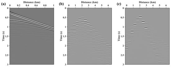
Figure 11.
The shot gathers from (a) towed streamer pressure component, (b) OBN vx component, and (c) OBN vz component.

Figure 12.
Frequency analysis of towed streamer and OBN data.
In Figure 13, we show the inversion results from the four methods. Although all methods can reconstruct the general structure of the velocity model, they exhibit notable differences in terms of spatial continuity and depth resolution. The inversion of the OBN data benefits from abundant S-wave and converted S-wave information, enabling accurate P- and S-wave velocity updates in deeper layers. However, limited sampling leads to low spatial continuity and visible acquisition footprints. The inversion of the towed streamer data is limited by the lack of low-frequency components and poor initial models, often resulting in local minima. Deep structures around 1 km show a huge deviation, and the S-wave velocity is updated incorrectly due to missing S-wave information.

Figure 13.
Inversion models. P-wave velocity inversion models: (a,c,e,g). S-wave velocity inversion models: (b,d,f,h). (a,b) OBN-only inversion results. (c,d) towed streamer-only inversion results. (e,f) J-AEFWI results. (g,h) PS-JFWI results.
Traditional J-AEFWI reduces shallow-layer problems, such as local minima in towed streamer data and footprints in OBN data, by combining both data types. However, it performs poorly in deeper layers due to gradient interference from towed streamer data. Analysis shows that, no matter how the data are weighted, S-wave gradients are still affected by P-wave gradients from the towed streamer data. In contrast, PS-JFWI employs a hierarchical strategy: in the first stage, we use OBN data to build a macro-scale velocity model, while in the second stage, we add the towed streamer data to optimize the shallow details. This approach enables joint reconstruction of both shallow and deep velocity structures. Even in the deep and complex structures, the recovered P- and S-wave models closely match the true models.
In order to present the differences among these four methods more intuitively, Figure 14 presents vertical velocity profiles at x = 1.0 km, 2.5 km, and 4.0 km. The towed streamer results (light blue curves) exhibit severe deviations due to local minima. OBN results (red curves) capture the overall velocity trends but lack resolution in localized structures. J-AEFWI (green curves) enhances shallow-layer accuracy but shows reduced performance in deeper regions compared with OBN-only inversion. In contrast, PS-JFWI (dark blue curves) achieves close agreement with the true models (black lines) across both shallow and deep layers, particularly near sharp velocity contrasts around 1.5 km depth. For quantitative evaluation, we used residual plots based on the Frobenius norm (Figure 15) and calculated their quantitative metrics (Table 1). These results show that the PS-JFWI method provides a useful way to combine the strengths from multiple data types.

Figure 14.
Vertical velocity profiles. (a–c): P-wave velocity model comparisons. (d–f): S-wave velocity model comparisons. (a,d) Traces at x = 1.0 km. (b,e) Traces at x = 2.5 km. (c,f) Traces at x = 4.0 km.

Figure 15.
Model residuals. P-wave velocity residuals: (a,c,e,g). S-wave velocity residuals: (b,d,f,h). (a,b) OBN-only inversion residuals. (c,d) towed streamer-only inversion residuals. (e,f) J-AEFWI residuals. (g,h) PS-JFWI residuals.

Table 1.
Percentage of model residuals.
Figure 16 shows the normalized misfit function curves of the four inversion methods. The EFWI using towed streamer data alone exhibits severe non-convergence after 90 iterations. The J-AEFWI method, which directly applies weighted processing to both data, also demonstrates non-convergence after 90 iterations, though less severe than the towed streamer-only results. The misfit curve for the OBN data remains stable and convergent throughout the multiscale iterative process. The PS-JFWI method completely overlaps with the OBN data curve during the first 45 iterations, corresponding to Stage I of the inversion strategy. Subsequently, benefiting from the incorporation of densely sampled towed streamer data and the P- and S-wave-separated gradient update strategy, its overall convergence rate is significantly accelerated.

Figure 16.
Normalized misfit function curves.
4. Discussion
Our study does not involve the estimation of density. However, in theory, EFWI is capable of simultaneously recovering P-wave velocity, S-wave velocity, and density. Actually, the inversion of density remains challenging. Previous work by Mora [40] demonstrated that the gradient kernels for and are difficult to distinguish in the presence of secondary scattering, resulting in strong coupling effects between and . Abubakar et al. proposed a compressed implicit Jacobian method for simultaneous inversion of multi-parameters [41]. However, the recovered density was far from the true model. Choi et al. implemented a frequency-domain EFWI method in acoustic-elastic coupled media and utilized low-frequency information to achieve relatively better inversion results for P-wave and S-wave velocities and density [42]. But acquiring and processing low-frequency data is challenging. Jeong et al. introduced a two-stage approach [43]. In the first stage, they updated the Lamé parameters, and in the second stage, they inverted for density and the Lamé parameter. This method somewhat mitigated the parameter coupling issue. Köhn et al. analyzed the impact of different elastic parameterization strategies on inversion results [44]. They found that Lamé parameterization led to severe artifacts, while velocity or impedance parameterizations produced fewer artifacts. Although these studies have made progress in density inversion, it remains a challenging problem. In future research, we need to further explore inversion algorithms to improve the accuracy of density inversion for better application in practical production.
It is also worth noting that this study is based on a 2D model for simplicity and computational feasibility. However, the main advantage of OBN data in real marine exploration lies in its full-azimuth coverage and full-wavefield vector recording in 3D space. Applying the method to 3D brings several challenges. Firstly, the computational complexity grows significantly because 3D models produce much larger datasets, demanding greater storage and processing power [45]. Secondly, in 3D, the inversion of parameters like and is more challenging due to stronger coupling, which leads to more obvious parameter crosstalk compared with 2D. Finally, the propagation of wavefields in 3D is more complex, particularly when dealing with wide-angle and full-wavefield data. Despite these challenges, 3D FWI is crucial for accurate marine modeling and improving the resolution of inversion results [46]. Future research could focus on extending the proposed method to 3D scenarios to better reflect practical acquisition conditions.
5. Conclusions
In this study, we explored a hierarchical joint FWI approach based on P- and S-wave separation (PS-JFWI) to improve the EFWI results using both towed streamer and OBN data. Numerical experiments demonstrate that the proposed method makes more effective use of the complementary characteristics of these two data. Compared with traditional joint inversion and single-data inversion approaches, PS-JFWI balances the contributions of different marine data by using gradient decoupling and the hierarchical inversion strategy, leading to an inversion result with higher accuracy. Quantitative evaluations further confirm the improvement: PS-JFWI achieves the lowest residuals between the inverted and true models among all tested methods, with P-wave and S-wave velocity errors reduced to 6.68% and 5.18%, respectively. These results suggest that PS-JFWI offers an effective way to enhance the stability and accuracy of multi-parameter EFWI in complex settings.
Author Contributions
Conceptualization, G.H. and J.H.; methodology, G.H. and J.H.; software, G.H.; validation, G.H.; formal analysis, G.H.; investigation, G.H.; resources, Y.L. and J.H.; data curation, G.H.; writing—original draft preparation, G.H.; writing—review and editing, Y.L.; visualization, G.H.; supervision, Y.L. and J.H.; project administration, Y.L. and J.H.; funding acquisition, Y.L. and J.H. All authors have read and agreed to the published version of the manuscript.
Funding
This study is supported by the National Natural Science Foundation of China (Grant No. 42374164), the High Precision Imaging Study of Small-scale and High-angle Structures in the Western Ordos Basin (Grant No. 2024D2ZZ01), the Imaging Study of Q Least Squares Migration (Grant No. 671024115010), the Research on Image Deconvolution Technology Based on Regularization (Grant No. 202418018212), the Research on the masked autoencoder method based on vit Network (Grant No. 30200020-24-ZC0613-0044), the National Natural Science Foundation of China (No. 42474153), the Natural Science Foundation of Shandong Province of China Outstanding Youth Science Fund Project (Overseas) (No. 2024HWYQ-046), TaiShan Scholars Project (No. tsqn20231214).
Data Availability Statement
The data presented in this study are available on request from the corresponding author.
Conflicts of Interest
The authors declare no conflicts of interest.
References
- Dagnino, D.; Sallarès, V.; Ranero, C.R. Waveform-preserving processing flow of multichannel seismic reflection data for adjoint-state full-waveform inversion of ocean thermohaline structure. IEEE Trans. Geosci. Remote Sens. 2017, 56, 1615–1625. [Google Scholar] [CrossRef]
- Kadu, A.; van Leeuwen, T.; Mulder, W.A. Salt reconstruction in full-waveform inversion with a parametric level-set method. IEEE Trans. Comput. Imaging 2016, 3, 305–315. [Google Scholar] [CrossRef]
- Yuan, S.; Liu, Y.; Zhang, Z.; Luo, C.; Wang, S. Prestack stochastic frequency-dependent velocity inversion with rock-physics constraints and statistical associated hydrocarbon attributes. IEEE Geosci. Remote Sens. Lett. 2018, 16, 140–144. [Google Scholar] [CrossRef]
- Li, Y.; Alkhalifah, T. Target-oriented time-lapse elastic full-waveform inversion constrained by deep learning-based prior model. IEEE Trans. Geosci. Remote Sens. 2022, 60, 1–12. [Google Scholar] [CrossRef]
- Tarantola, A. Inversion of seismic reflection data in the acoustic approximation. Geophysics 1984, 49, 1259–1266. [Google Scholar] [CrossRef]
- Lailly, P.; Bednar, J. The seismic inverse problem as a sequence of before stack migrations. In Conference on Inverse Scattering: Theory and Application; SIAM: Philadelphia, PA, USA, 1983; Volume 1983, pp. 206–220. [Google Scholar]
- Pratt, R.G. Seismic waveform inversion in the frequency domain, Part 1: Theory and verification in a physical scale model. Geophysics 1999, 64, 888–901. [Google Scholar] [CrossRef]
- Operto, S.; Gholami, Y.; Prieux, V.; Ribodetti, A.; Brossier, R.; Métivier, L.; Virieux, J. A guided tour of multiparameter full-waveform inversion with multicomponent data: From theory to practice. Lead. Edge 2013, 32, 1040–1054. [Google Scholar] [CrossRef]
- Barnes, C.; Charara, M. Full-waveform inversion results when using acoustic approximation instead of elastic medium. In Proceedings of the 70th EAGE Conference and Exhibition-Workshops and Fieldtrips, Rome, Italy, 9–12 June 2008; European Association of Geoscientists & Engineers: Utrecht, The Netherlands, 2008; p. cp-41-00067. [Google Scholar]
- Brossier, R.; Operto, S.; Virieux, J. Seismic imaging of complex onshore structures by 2D elastic frequency-domain full-waveform inversion. Geophysics 2009, 74, WCC105–WCC118. [Google Scholar] [CrossRef]
- Xu, K.; McMechan, G.A. 2D frequency-domain elastic full-waveform inversion using time-domain modeling and a multistep-length gradient approach. Geophysics 2014, 79, R41–R53. [Google Scholar] [CrossRef]
- Manukyan, E.; Maurer, H.; Nuber, A. Improvements to elastic full-waveform inversion using cross-gradient constraints. Geophysics 2018, 83, R105–R115. [Google Scholar] [CrossRef]
- Wang, T.; Cheng, J. Elastic full waveform inversion based on mode decomposition: The approach and mechanism. Geophys. J. Int. 2017, 209, 606–622. [Google Scholar] [CrossRef]
- Hu, Y.; Fu, L.Y.; Li, Q.; Deng, W.; Han, L. Frequency-wavenumber domain elastic full waveform inversion with a multistage phase correction. Remote Sens. 2022, 14, 5916. [Google Scholar] [CrossRef]
- Forgues, E.; Lambaré, G. Parameterization study for acoustic and elastic ray plus born inversion. J. Seism. Explor. 1997, 6, 253–277. [Google Scholar]
- Tarantola, A. A strategy for nonlinear elastic inversion of seismic reflection data. Geophysics 1986, 51, 1893–1903. [Google Scholar] [CrossRef]
- Wang, T.; Cheng, J. Elastic wave mode decoupling for full waveform inversion. In Proceedings of the SEG International Exposition and Annual Meeting, SEG, New Orleans, LA, USA, 18–23 October 2015; p. SEG-2015-5914394. [Google Scholar]
- Ren, Z.; Liu, Y. A hierarchical elastic full-waveform inversion scheme based on wavefield separation and the multistep-length approach. Geophysics 2016, 81, R99–R123. [Google Scholar] [CrossRef]
- Agudo, Ò.C.; da Silva, N.V.; Warner, M.; Morgan, J. Acoustic full-waveform inversion in an elastic world. Geophysics 2018, 83, R257–R271. [Google Scholar] [CrossRef]
- Sun, M.; Jin, S. Multiparameter elastic full waveform inversion of ocean bottom seismic four-component data based on a modified acoustic-elastic coupled equation. Remote Sens. 2020, 12, 2816. [Google Scholar] [CrossRef]
- Plotnitskii, P.; Ovcharenko, O.; Kazei, V.; Peter, D.; Alkhalifah, T. Deep learning enhanced initial model prediction in elastic FWI: Application to marine streamer data. arXiv 2025, arXiv:2501.12992. [Google Scholar]
- Yu, P.; Geng, J.; Li, X.; Wang, C. Acoustic-elastic coupled equation for ocean bottom seismic data elastic reverse time migration. Geophysics 2016, 81, S333–S345. [Google Scholar] [CrossRef]
- Hondori, E.J.; Mikada, H.; Asakawa, E.; Mizohata, S. A new initial model for full waveform inversion without cycle skipping. In Proceedings of the SEG International Exposition and Annual Meeting, SEG, New Orleans, LA, USA, 18–23 October 2015; p. SEG-2015-5895875. [Google Scholar]
- Yao, G.; da Silva, N.V.; Warner, M.; Wu, D.; Yang, C. Tackling cycle skipping in full-waveform inversion with intermediate data. Geophysics 2019, 84, R411–R427. [Google Scholar] [CrossRef]
- Shen, X. Near-surface velocity estimation by weighted early-arrival waveform inversion. In Proceedings of the SEG International Exposition and Annual Meeting, SEG, Denver, CO, USA, 17–22 October 2010; p. SEG-2010-1975. [Google Scholar]
- Wang, G.; Yuan, S.; Wang, S. Retrieving low-wavenumber information in FWI: An efficient solution for cycle skipping. IEEE Geosci. Remote Sens. Lett. 2019, 16, 1125–1129. [Google Scholar] [CrossRef]
- Song, C.; Feng, X.; Gao, Y.; Li, B.; Liu, C. Elastic wavefield reconstruction inversion with source estimation. IEEE Trans. Geosci. Remote Sens. 2023, 62, 1–9. [Google Scholar] [CrossRef]
- Sears, T.J.; Singh, S.; Barton, P. Elastic full waveform inversion of multi-component OBC seismic data. Geophys. Prospect. 2008, 56, 843–862. [Google Scholar] [CrossRef]
- Cheng, S.; Shi, X.; Mao, W.; Alkhalifah, T.A.; Yang, T.; Liu, Y.; Sun, H. Elastic seismic imaging enhancement of sparse 4C ocean-bottom node data using deep learning. IEEE Trans. Geosci. Remote Sens. 2023, 61, 1–14. [Google Scholar] [CrossRef]
- Faucher, F.; Alessandrini, G.; Barucq, H.; de Hoop, M.V.; Gaburro, R.; Sincich, E. Full reciprocity-gap waveform inversion enabling sparse-source acquisition. Geophysics 2020, 85, R461–R476. [Google Scholar] [CrossRef]
- Yu, P.; Geng, J.; Ma, J. Vector-wave-based elastic reverse time migration of ocean-bottom 4C seismic data. Geophysics 2018, 83, S333–S343. [Google Scholar] [CrossRef]
- Virieux, J.; Operto, S. An overview of full-waveform inversion in exploration geophysics. Geophysics 2009, 74, WCC1–WCC26. [Google Scholar] [CrossRef]
- Yang, T.; Liu, Y.; Yang, J. Joint towed streamer and ocean-bottom-seismometer data multi-parameter full waveform inversion in acoustic-elastic coupled media. Front. Earth Sci. 2023, 10, 1085441. [Google Scholar] [CrossRef]
- Lanzarone, P.; Shen, X.; Brenders, A.; Xia, G.; Dellinger, J.; Ritter, G.; Etgen, J. Innovative application of full-waveform inversion applied to extended wide-azimuth marine streamer seismic data in a complex salt environment. Geophysics 2022, 87, B193–B205. [Google Scholar] [CrossRef]
- Yang, H.; Zhang, J. Full waveform inversion of combined towed streamer and limited OBS seismic data: A theoretical study. Mar. Geophys. Res. 2019, 40, 237–244. [Google Scholar] [CrossRef]
- Yang, H.; Zhang, J.; Wu, Z.; Huang, Z.L. Joint reverse-time imaging condition of seismic towed-streamer and OBN data. IEEE Geosci. Remote Sens. Lett. 2022, 19, 1–5. [Google Scholar] [CrossRef]
- Yu, P.; Chu, M.; Xu, Y.; Zhang, B.; Geng, J. Joint elastic reverse time migration of towed streamer and sparse ocean-bottom seismic node hybrid data. Geophysics 2023, 88, S47–S57. [Google Scholar] [CrossRef]
- Jianlei, Z.; Zhenping, T.; Chengxiang, W. P-and S-wave separated elastic wave equation numerical modeling using 2D staggered-grid. In Proceedings of the SEG International Exposition and Annual Meeting, SEG, San Antonio, TX, USA, 23–28 September 2007; p. SEG-2007-2104. [Google Scholar]
- Plessix, R.E. A review of the adjoint-state method for computing the gradient of a functional with geophysical applications. Geophys. J. Int. 2006, 167, 495–503. [Google Scholar] [CrossRef]
- Mora, P. Nonlinear two-dimensional elastic inversion of multioffset seismic data. Geophysics 1987, 52, 1211–1228. [Google Scholar] [CrossRef]
- Abubakar, A.; Li, M.; Lin, Y.; Habashy, T. Compressed implicit Jacobian scheme for elastic full-waveform inversion. Geophys. J. Int. 2012, 189, 1626–1634. [Google Scholar] [CrossRef][Green Version]
- Choi, Y.; Min, D.J.; Shin, C. Two-dimensional waveform inversion of multi-component data in acoustic-elastic coupled media. Geophys. Prospect. 2008, 56, 863–881. [Google Scholar] [CrossRef]
- Jeong, W.; Lee, H.Y.; Min, D.J. Full waveform inversion strategy for density in the frequency domain. Geophys. J. Int. 2012, 188, 1221–1242. [Google Scholar] [CrossRef]
- Köhn, D.; De Nil, D.; Kurzmann, A.; Przebindowska, A.; Bohlen, T. On the influence of model parametrization in elastic full waveform tomography. Geophys. J. Int. 2012, 191, 325–345. [Google Scholar] [CrossRef]
- Warner, M.; Ratcliffe, A.; Nangoo, T.; Morgan, J.; Umpleby, A.; Shah, N.; Vinje, V.; Štekl, I.; Guasch, L.; Win, C.; et al. Anisotropic 3D full-waveform inversion. Geophysics 2013, 78, R59–R80. [Google Scholar] [CrossRef]
- Wang, Z.Y.; Huang, J.P.; Liu, D.J.; Li, Z.C.; Yong, P.; Yang, Z.J. 3D variable-grid full-waveform inversion on GPU. Petrol. Sci. 2019, 16, 1001–1014. [Google Scholar] [CrossRef]
Disclaimer/Publisher’s Note: The statements, opinions and data contained in all publications are solely those of the individual author(s) and contributor(s) and not of MDPI and/or the editor(s). MDPI and/or the editor(s) disclaim responsibility for any injury to people or property resulting from any ideas, methods, instructions or products referred to in the content. |
© 2025 by the authors. Licensee MDPI, Basel, Switzerland. This article is an open access article distributed under the terms and conditions of the Creative Commons Attribution (CC BY) license (https://creativecommons.org/licenses/by/4.0/).