


Use of Machine-Learning Techniques to Estimate Long-Term Wave Power at a Target Site Where Short-Term Data Are Available


Abstract
1. Introduction
1.1. Aims and Originality of This Paper
1.2. Structure of the Paper
2. Materials
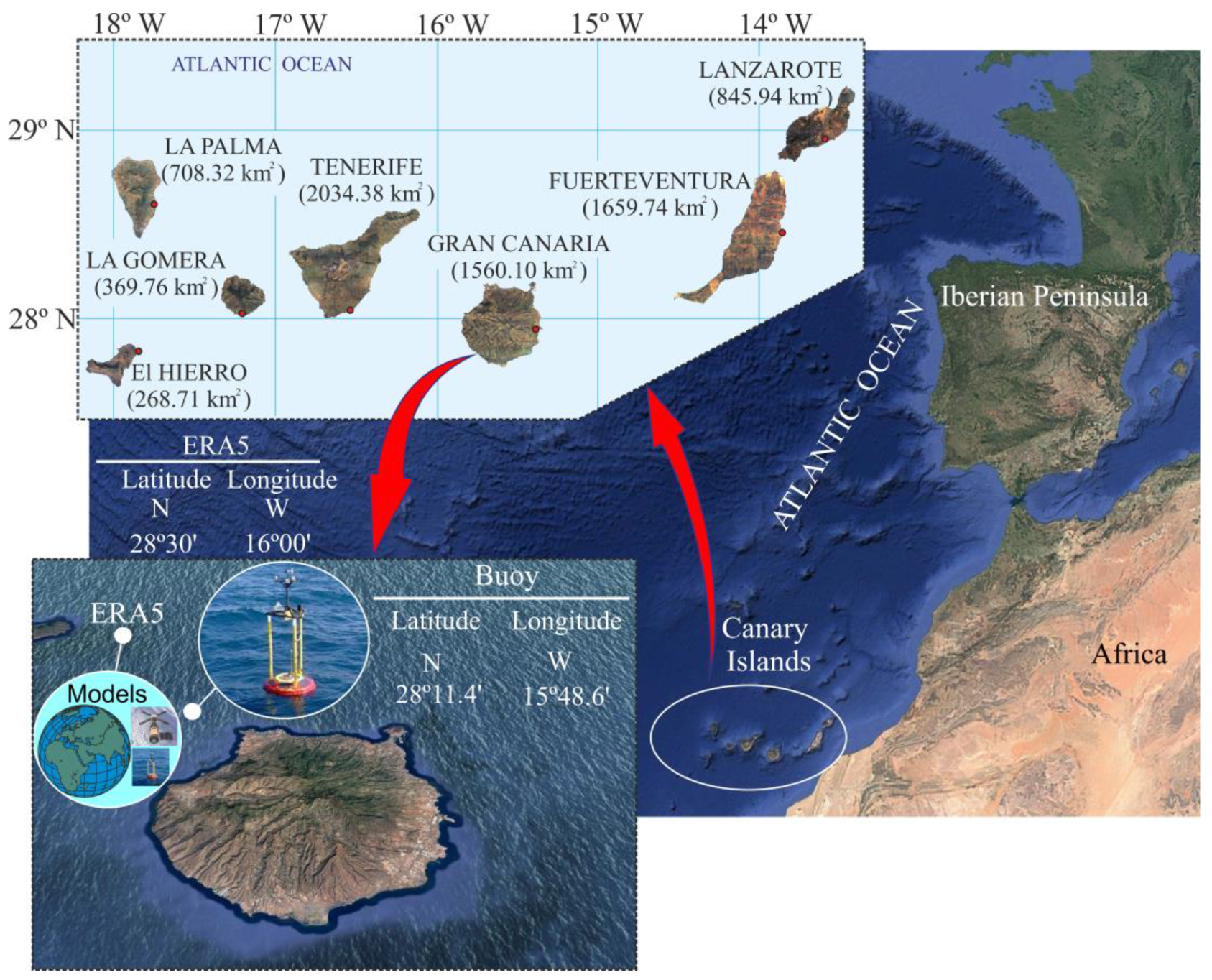
2.1. Background
- (a)
- Its geographical remoteness, which greatly hinders interconnection with the large energy supply networks of continental territories.
- (b)
- A lack of conventional energy sources, resulting in an almost total dependence on external supplies, primarily petroleum-based.
- (c)
- Its high wind and solar energy potential.
2.2. Data Used
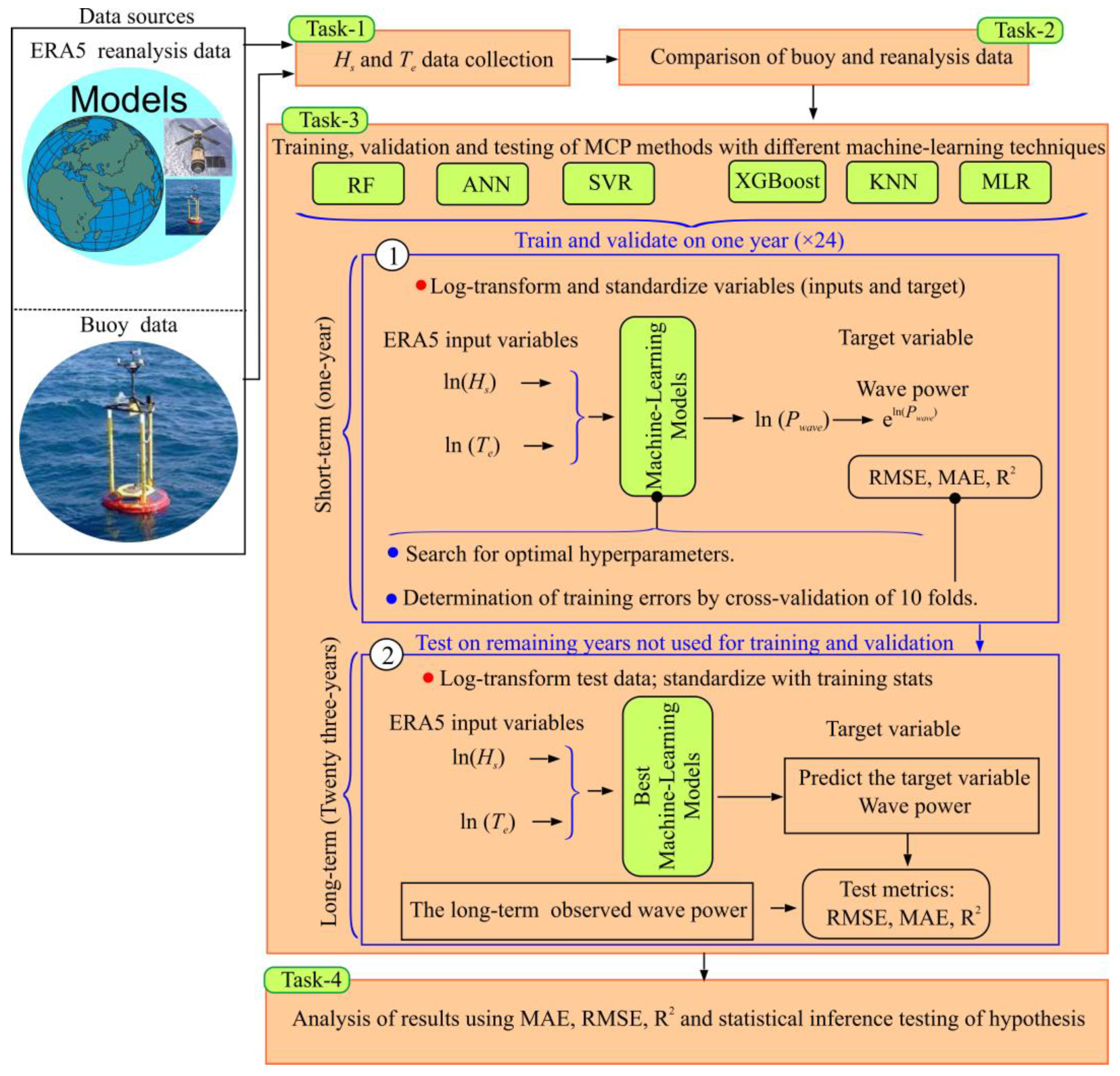
3. Method
3.1. Task 1 of the Method
3.2. Task 2 of the Method
3.3. Task 3 of the Method
- MLR: A baseline linear model that assumes additive relationships between the inputs and the output.
- SVR: A non-linear model that identifies optimal hyperplanes in a transformed feature space, suitable for capturing complex patterns.
- KNN: A distance-based algorithm that predicts output values by averaging the nearest training points in the feature space.
- RF: An ensemble of decision trees trained on bootstrapped subsets of the data to enhance robustness and reduce overfitting.
- XGBoost: A powerful boosting technique that builds trees sequentially to correct the errors of previous trees.
- ANN: Layered computational models capable of learning non-linear relationships through training across multiple hidden units.
3.4. Task 4 of the Method
4. Results and Discussion
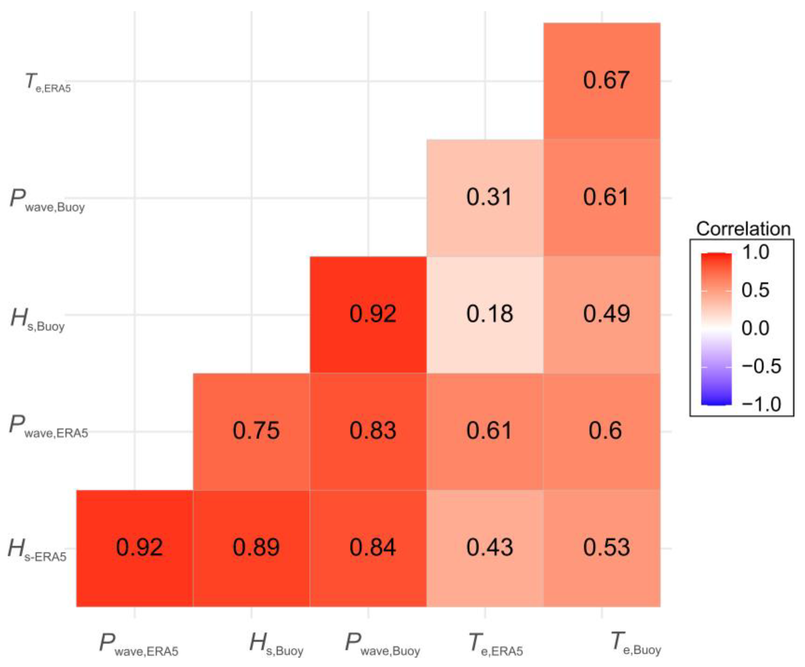
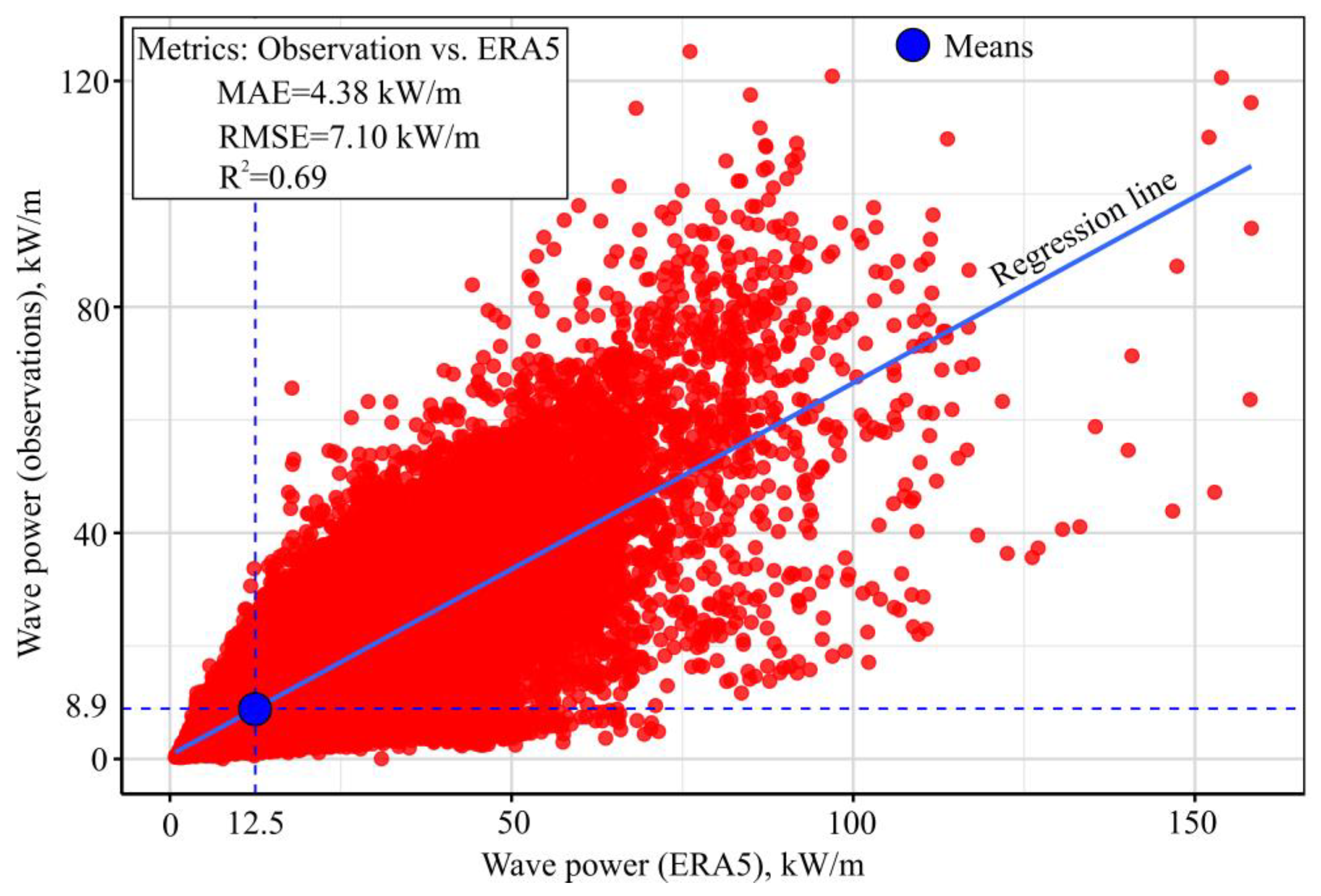
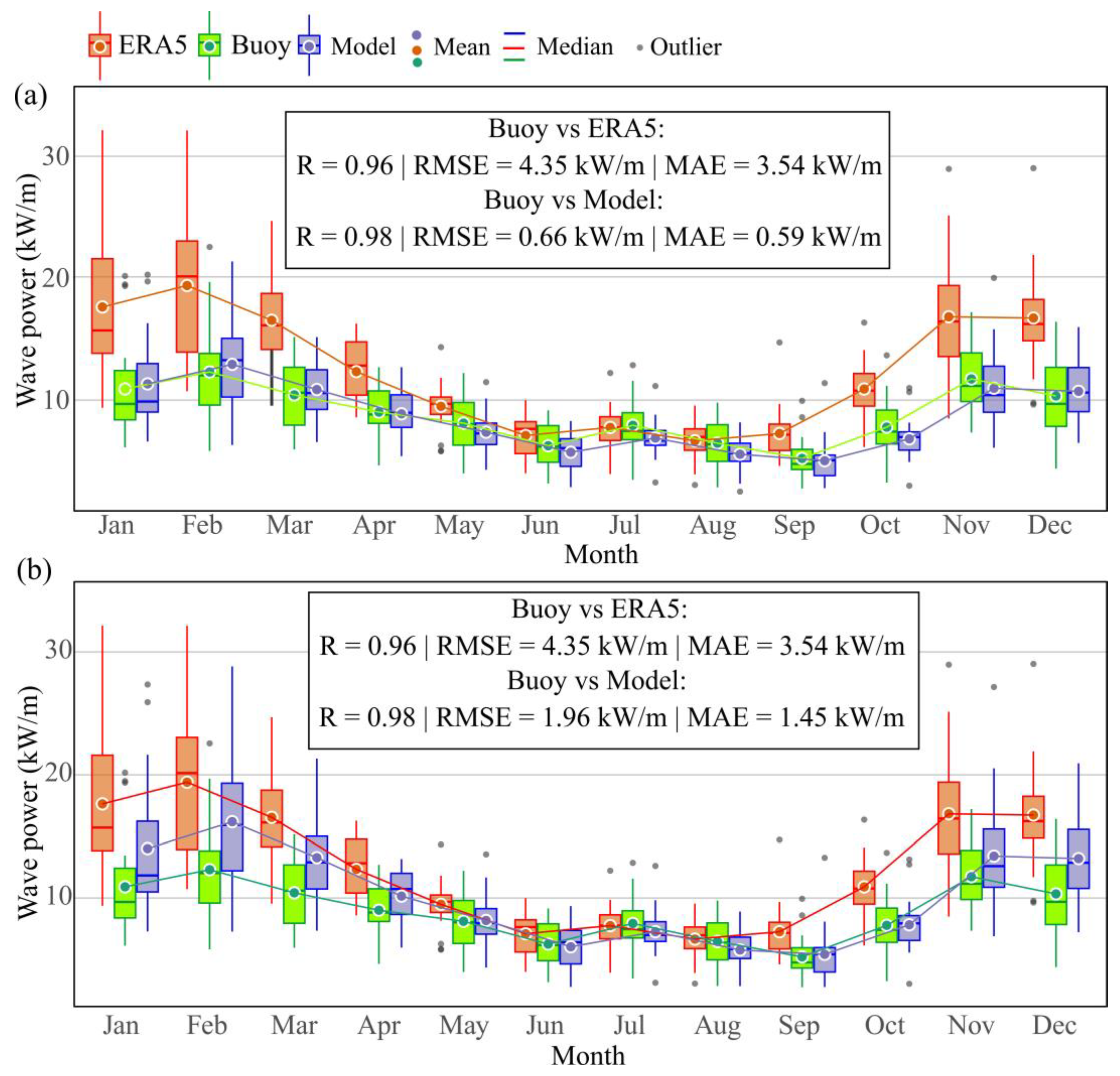
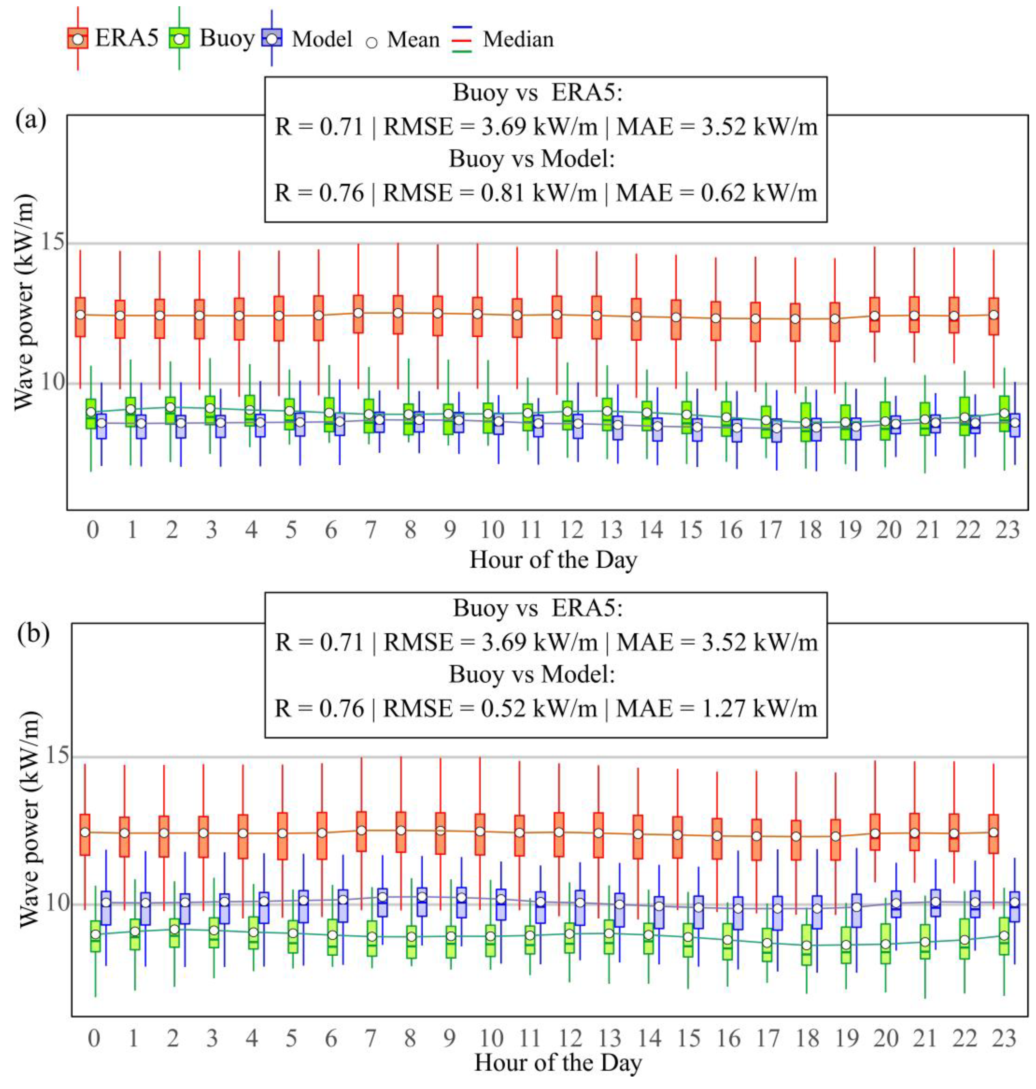
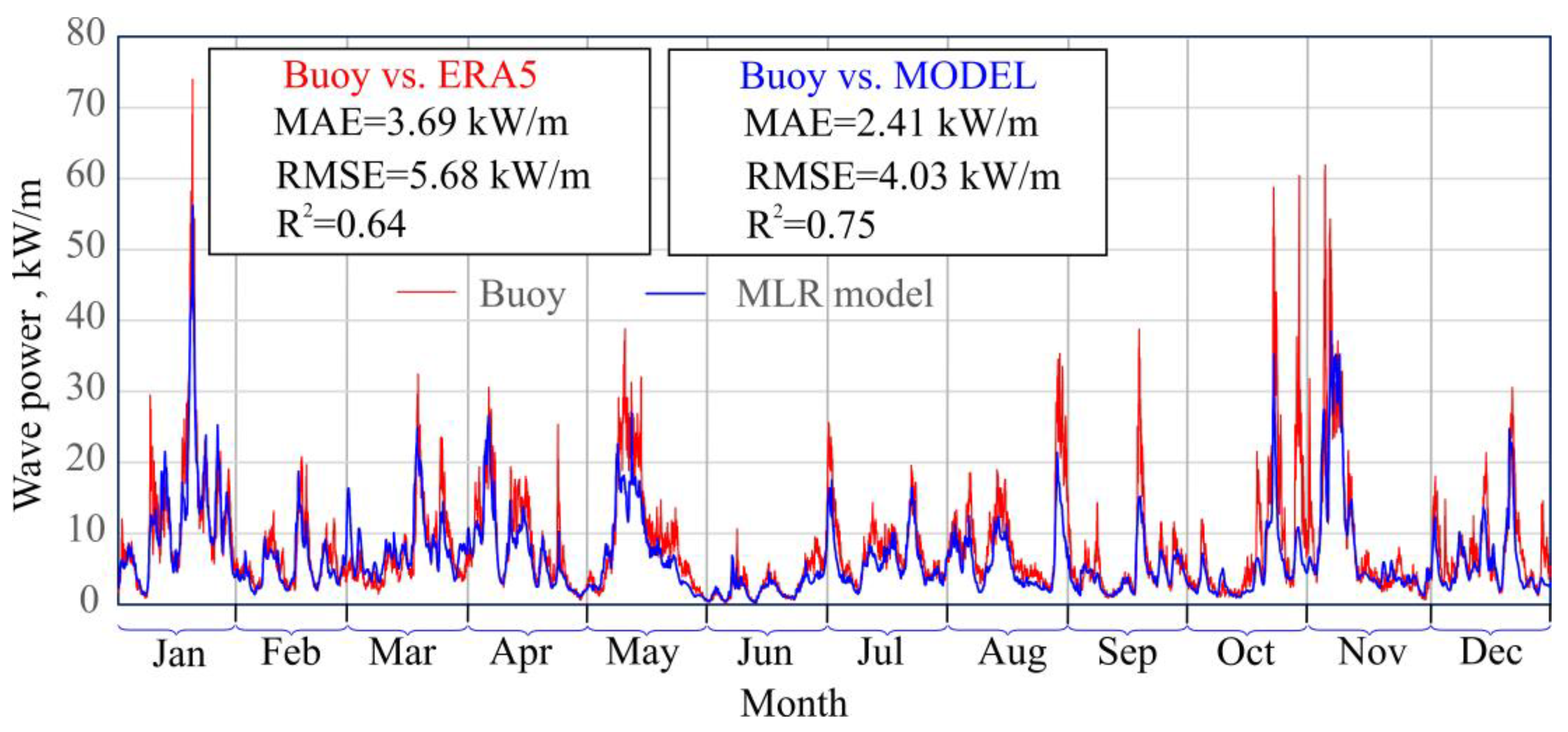
4.1. Comparison of the Data Recorded in the Two Data Sources
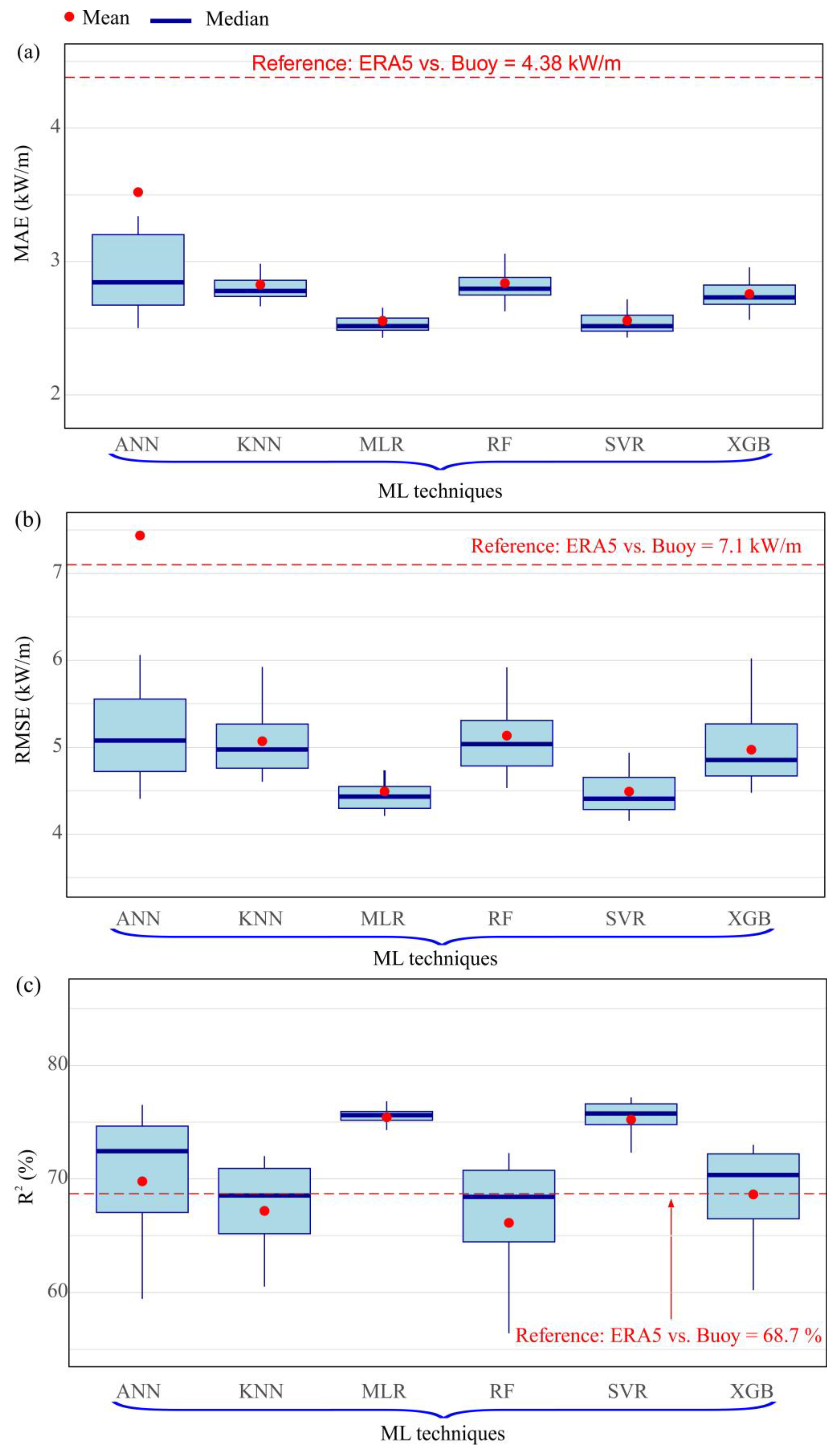
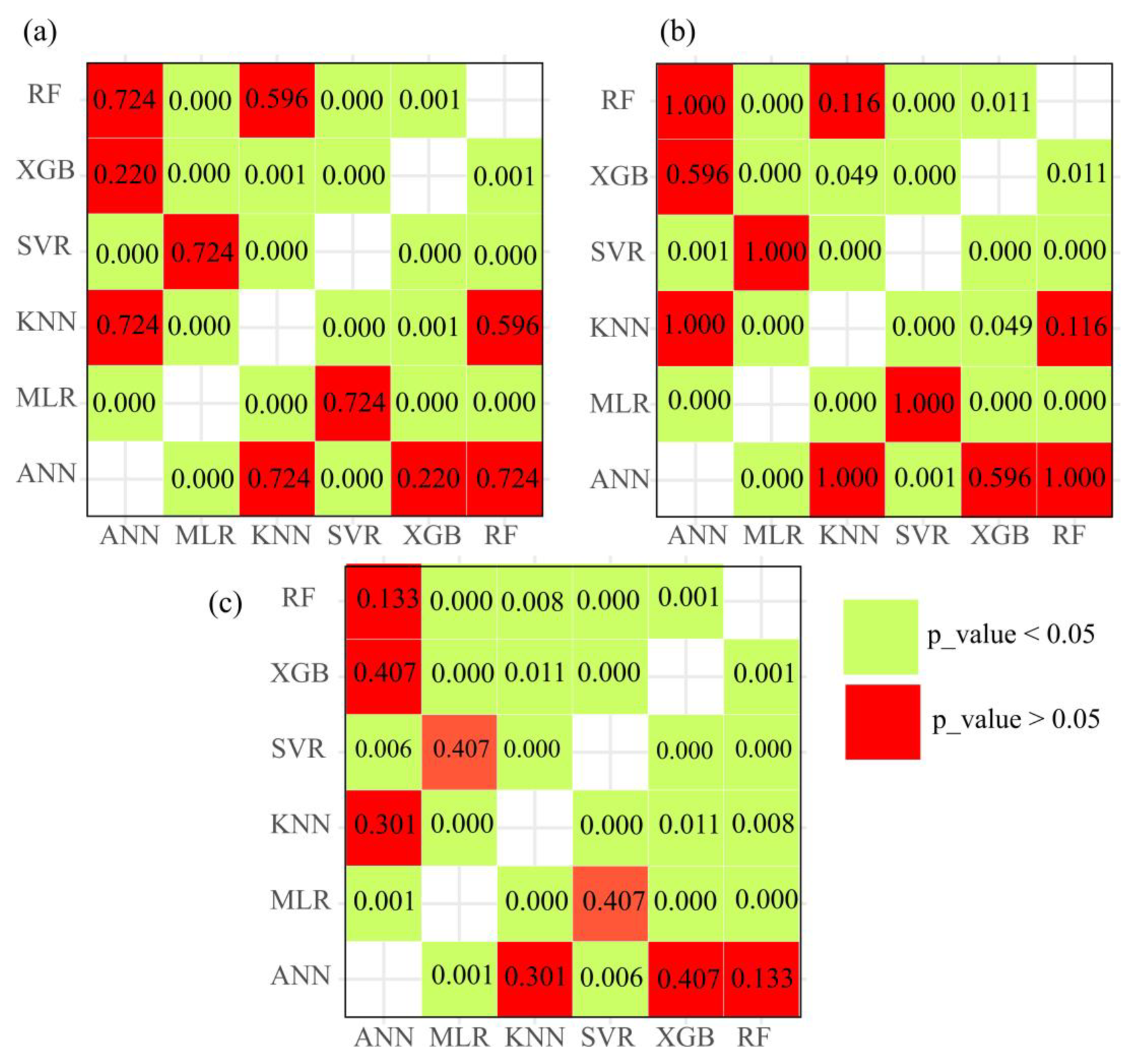
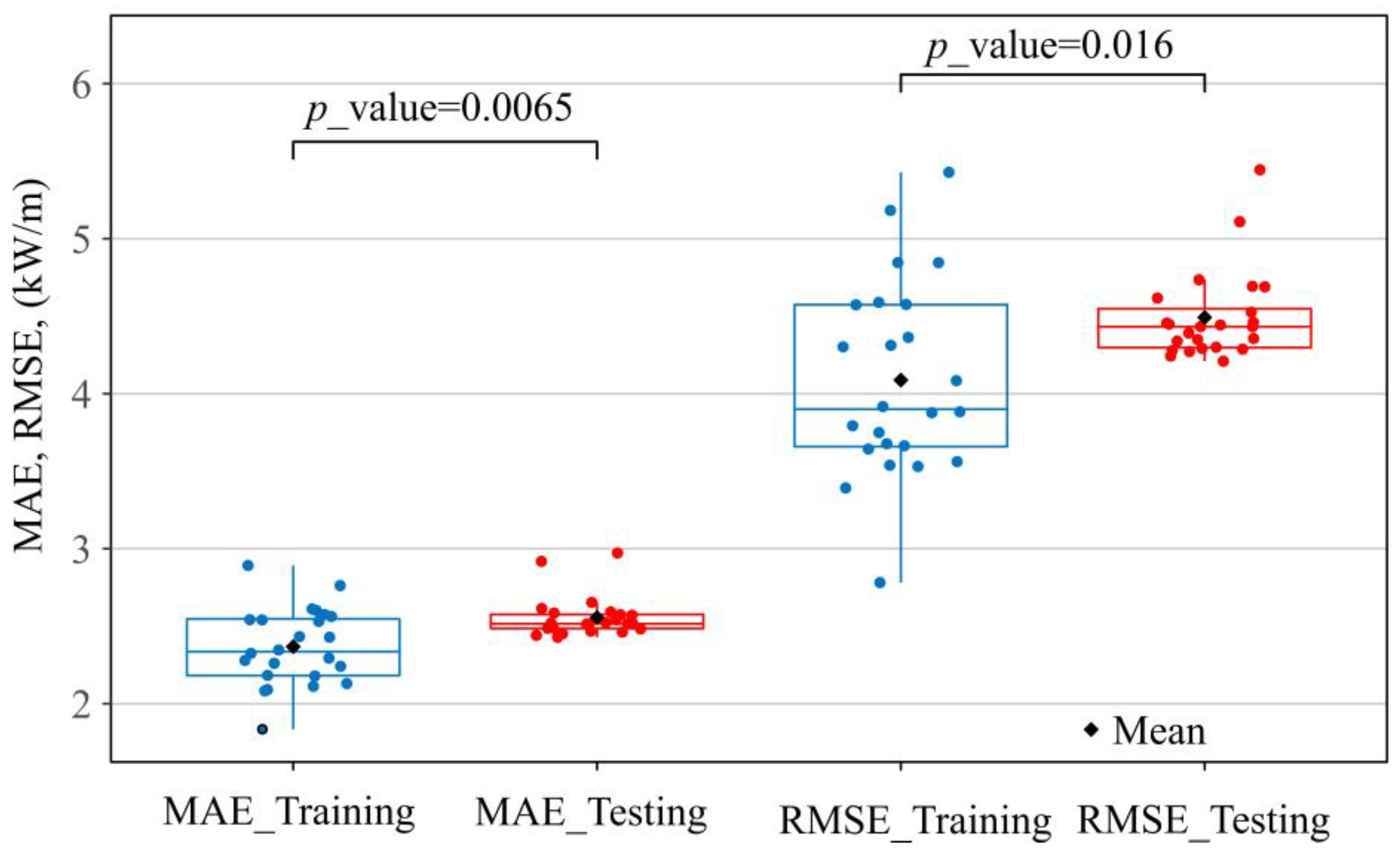
4.2. Results Obtained from the MCP Models
5. Conclusions
- ERA5 reanalysis data systematically overestimate wave power compared to buoy observations, especially during high-energy months, and fail to accurately capture the daily and seasonal variability at the target site.
- Machine-learning techniques—particularly MLR and SVR—substantially improve wave power estimation, reducing error metrics (MAE, RMSE) and increasing the coefficient of determination (R2) relative to ERA5-based predictions.
- The MLR model offers a key advantage through its interpretable power-law form, enabling direct analysis of how ERA5 variables influence wave power estimates. The parameters A, b, and c provide insight into calibration bias and variable sensitivity, bridging data-driven modeling with physical understanding.
- The approach demonstrates strong temporal robustness, with MLR models trained on early-period data (e.g., 2000) still outperforming ERA5 when applied to recent years (e.g., 2023), even under evolving wave conditions.
- The methodology is fully reproducible and transferable to other coastal regions, relying on openly available reanalysis data and implemented entirely with transparent R-based tools, which supports its adoption in data-limited marine energy assessments.
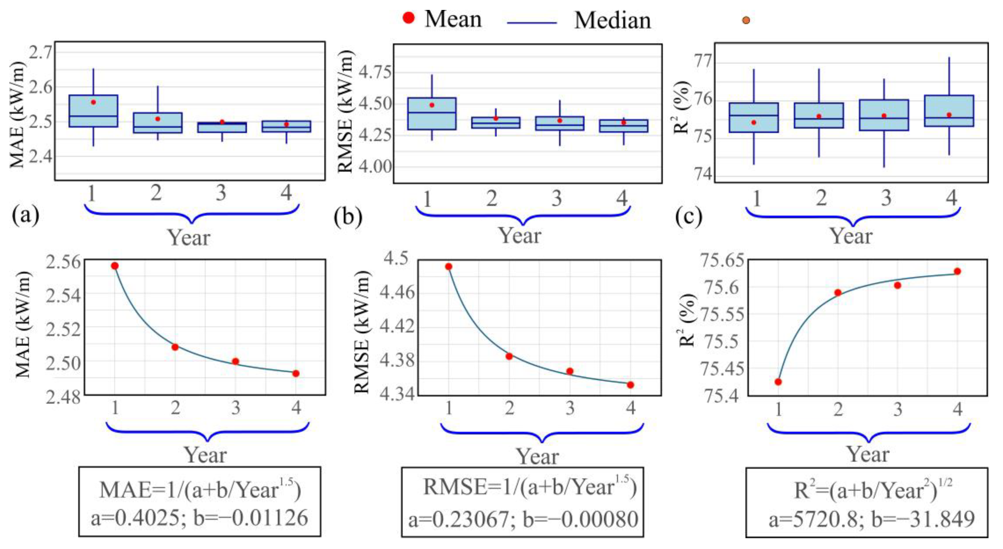
- Additionally, in this case study, extending the training period from one to four years resulted in slight improvements in model performance. While this suggests that longer measurement campaigns may offer marginal benefits, such conclusions should be validated on a site-specific basis and balanced against the increased cost of data acquisition.
Author Contributions
Funding
Data Availability Statement
Acknowledgments
Conflicts of Interest
Abbreviations
| ANN | Artificial Neural Network |
| ERA5 | European Centre for Medium-Range Weather Forecasts Reanalysis |
| GW | GigaWatts |
| Hs | Significant wave height |
| IRENA | International Renewable Energy Agency |
| KNN | K-Nearest-Neighbor |
| KW/m | KiloWatts per meter |
| MAE | Mean absolute error |
| MCP | Measure–Correlate–Predict |
| ML | Machine learning |
| MLR | Multiple Linear Regression |
| PLOCAN | PLataforma Oceánica de CANarias—Oceanic Platform of the Canary Islands |
| PTECAN | Plan de Transición Energética de CANarias—Canary Islands’ Energy Transition Plan |
| Pwave | Wave power |
| RF | Random Forest |
| R2 | Coefficient of determination |
| RMSE | Root mean squared error |
| SVR | Support Vector Regression |
| Te | Energy period |
| Tp | Peak period |
| XGBoost | eXtreme Gradient Boosting |
Appendix A

| Year | RF Parameters | ANN Parameters | ||||
|---|---|---|---|---|---|---|
| Mtry | Trees | Max_Depth | Hidden Layers | Epochs | Neurons per Layer | |
| 2000 | 1 | 3000 | 30 | 1 | 604 | 2 |
| 2001 | 1 | 3000 | 30 | 1 | 1004 | 5 |
| 2002 | 1 | 3000 | 30 | 2 | 904 | 9-9 |
| 2003 | 1 | 3000 | 30 | 1 | 604 | 2 |
| 2004 | 1 | 3000 | 7 | 1 | 1004 | 9 |
| 2005 | 1 | 3000 | 30 | 1 | 904 | 8 |
| 2006 | 1 | 3000 | 30 | 2 | 804 | 6-6 |
| 2007 | 1 | 3000 | 30 | 2 | 504 | 8-8 |
| 2008 | 1 | 3000 | 7 | 2 | 903 | 3-2 |
| 2009 | 1 | 3000 | 30 | 1 | 704 | 2 |
| 2010 | 1 | 3000 | 30 | 1 | 904 | 3 |
| 2011 | 1 | 3000 | 30 | 2 | 905 | 5-5 |
| 2012 | 1 | 3000 | 30 | 1 | 604 | 3 |
| 2013 | 1 | 3000 | 30 | 2 | 1003 | 4-2 |
| 2014 | 1 | 3000 | 30 | 1 | 804 | 10 |
| 2015 | 1 | 3000 | 30 | 2 | 904 | 6-6 |
| 2016 | 1 | 3000 | 30 | 2 | 804 | 4-4 |
| 2017 | 1 | 3000 | 30 | 2 | 1004 | 3-2 |
| 2018 | 1 | 3000 | 30 | 1 | 803 | 2 |
| 2019 | 1 | 3000 | 30 | 2 | 504 | 10-10 |
| 2020 | 1 | 3000 | 30 | 2 | 1005 | 3-3 |
| 2021 | 1 | 3000 | 30 | 2 | 904 | 4-3 |
| 2022 | 1 | 3000 | 30 | 1 | 603 | 12 |
| 2023 | 1 | 3000 | 30 | 2 | 504 | 8-8 |
| Year | SVR Parameters | XGBoost Parameters | |||||
|---|---|---|---|---|---|---|---|
| σ | C | ε | Min_n | Tree.Depth | Learn_Rate | Loss.Reduction | |
| 2000 | 0.01 | 1 | 0.001 | 8 | 8 | 0.0052511 | 5.85 × 10⁻⁵ |
| 2001 | 0.01 | 1 | 0.001 | 30 | 13 | 0.00989746 | 0.34308064 |
| 2002 | 0.01 | 1 | 0.001 | 11 | 10 | 0.00602343 | 7.83 × 10⁻⁸ |
| 2003 | 0.01 | 1 | 0.001 | 20 | 9 | 0.00746615 | 1.06 × 10⁻¹⁰ |
| 2004 | 0.01 | 1 | 0.001 | 15 | 5 | 0.09011734 | 0.04092907 |
| 2005 | 0.01 | 1 | 0.001 | 8 | 8 | 0.00515634 | 1.74 × 10⁻¹⁰ |
| 2006 | 0.01 | 1 | 0.001 | 21 | 11 | 0.01865139 | 0.8246732 |
| 2007 | 0.01 | 1 | 0.001 | 4 | 6 | 0.00828647 | 6.40 × 10⁻¹⁰ |
| 2008 | 0.01 | 1 | 0.001 | 28 | 11 | 0.03561075 | 0.07489249 |
| 2009 | 0.01 | 1 | 0.001 | 36 | 7 | 0.05246322 | 0.10571014 |
| 2010 | 0.01 | 1 | 0.001 | 18 | 10 | 0.0075247 | 2.95 × 10⁻⁶ |
| 2011 | 0.01 | 1 | 0.001 | 33 | 11 | 0.0079609 | 4.80 × 10⁻⁷ |
| 2012 | 0.01 | 1 | 0.001 | 19 | 12 | 0.00557426 | 3.80 × 10⁻⁹ |
| 2013 | 0.01 | 1 | 0.001 | 35 | 15 | 0.00771763 | 0.26072018 |
| 2014 | 0.01 | 1 | 0.001 | 3 | 9 | 0.06530932 | 0.11592727 |
| 2015 | 0.01 | 1 | 0.001 | 23 | 13 | 0.00589396 | 5.01 × 10⁻⁹ |
| 2016 | 0.01 | 1 | 0.001 | 36 | 7 | 0.05246322 | 0.10571014 |
| 2017 | 0.01 | 1 | 0.001 | 21 | 11 | 0.01865139 | 0.8246732 |
| 2018 | 0.01 | 1 | 0.001 | 15 | 8 | 0.00967407 | 2.57 × 10⁻⁷ |
| 2019 | 0.01 | 1 | 0.001 | 27 | 11 | 0.04011186 | 0.15475962 |
| 2020 | 0.01 | 1 | 0.001 | 16 | 12 | 0.00437732 | 0.00017414 |
| 2021 | 0.001 | 1 | 0.001 | 15 | 14 | 0.0055972 | 1.29 × 10⁻⁷ |
| 2022 | 0.01 | 1 | 0.001 | 21 | 12 | 0.03830943 | 0.07938781 |
| 2023 | 0.01 | 1 | 0.001 | 32 | 11 | 0.00494699 | 0.00513382 |
| Year | KNN Parameters | ||||
|---|---|---|---|---|---|
| Neighbors | weight_func | deg_free_H | deg_free_T | Neighbors | |
| 2000 | 26 | triangular | 18 | 18 | 26 |
| 2001 | 37 | triangular | 2 | 4 | 37 |
| 2002 | 39 | triweight | 5 | 6 | 39 |
| 2003 | 26 | biweight | 16 | 17 | 26 |
| 2004 | 36 | triweight | 15 | 18 | 36 |
| 2005 | 14 | biweight | 2 | 2 | 14 |
| 2006 | 34 | triweight | 2 | 3 | 34 |
| 2007 | 30 | triweight | 4 | 4 | 30 |
| 2008 | 50 | biweight | 17 | 14 | 50 |
| 2009 | 20 | optimal | 3 | 2 | 20 |
| 2010 | 40 | triweight | 2 | 2 | 40 |
| 2011 | 31 | triweight | 10 | 12 | 31 |
| 2012 | 41 | biweight | 10 | 11 | 41 |
| 2013 | 41 | triweight | 7 | 8 | 41 |
| 2014 | 50 | triangular | 10 | 10 | 50 |
| 2015 | 23 | biweight | 3 | 2 | 23 |
| 2016 | 36 | biweight | 2 | 3 | 36 |
| 2017 | 50 | triangular | 10 | 10 | 50 |
| 2018 | 33 | biweight | 18 | 18 | 33 |
| 2019 | 22 | triangular | 4 | 3 | 22 |
| 2020 | 14 | inv | 18 | 18 | 14 |
| 2021 | 14 | inv | 18 | 18 | 14 |
| 2022 | 50 | triweight | 13 | 17 | 50 |
| 2023 | 47 | triweight | 14 | 11 | 47 |
Appendix B
| 1 | www.gobiernodecanarias.org/energia/info-publica/PTECan_VersionInicial/, accessed on 7 May 2025 |
| 2 | https://plocan.eu/, accessed on 7 May 2025 |
References
- Renewable Energy in Climate Change Adaptation: Metrics and Risk Assessment Framework. Available online: https://www.irena.org/Publications/2025/Apr/Renewable-energy-in-climate-change-adaptation (accessed on 24 April 2025).
- International Renewable Energy Agency. Renewable Capacity Highlights 2025. 2025. Available online: https://unstats.un.org/unsd/methodology/m49/ (accessed on 24 April 2025).
- International Renewable Energy Agency. OCEAN ENERGY TECHNOLOGIES A Brief from the IRENA Collaborative Framework on Ocean Energy and Offshore Renewables. 2023. Available online: www.irena.org (accessed on 24 April 2025).
- International Renewable Energy Agency. World Energy Transitions Outlook 2022: 1.5 °C Pathway. Available online: www.irena.org/publications/2022/Mar/World-Energy-Transitions-Outlook-2022 (accessed on 24 April 2025).
- Sun, P.; Wang, J. Long-term variability analysis of wave energy resources and its impact on wave energy converters along the Chinese coastline. Energy 2024, 288, 129644. [Google Scholar] [CrossRef]
- Khojasteh, D.; Mousavi, S.M.; Glamore, W.; Iglesias, G. Wave energy status in Asia. Ocean. Eng. 2018, 169, 344–358. [Google Scholar] [CrossRef]
- Astariz, S.; Iglesias, G. The economics of wave energy: A review. Renew. Sustain. Energy Rev. 2015, 45, 397–408. [Google Scholar] [CrossRef]
- Satymov, R.; Bogdanov, D.; Dadashi, M.; Lavidas, G.; Breyer, C. Techno-economic assessment of global and regional wave energy resource potentials and profiles in hourly resolution. Appl. Energy 2024, 364, 123119. [Google Scholar] [CrossRef]
- Majidi, A.G.; Ramos, V.; Rosa-Santos, P.; Akpınar, A.; Neves, L.D.; Taveira-Pinto, F. Development of a multi-criteria decision-making tool for combined offshore wind and wave energy site selection. Appl. Energy 2025, 384, 125422. [Google Scholar] [CrossRef]
- Silva, K.; Abreu, T.; Oliveira, T.C.A. Inter- and intra-annual variability of wave energy in Northern mainland Portugal: Application to the HiWave-5 project. Energy Rep. 2022, 8, 6411–6422. [Google Scholar] [CrossRef]
- Tong, Y.; Li, J.; Chen, W.; Li, B. Long-Term (1979–2024) Variation Trend in Wave Power in the South China Sea. J. Mar. Sci. Eng. 2025, 13, 524. [Google Scholar] [CrossRef]
- Reguero, B.G.; Losada, I.J.; Méndez, F.J. A global wave power resource and its seasonal, interannual and long-term variability. Appl. Energy 2015, 148, 366–380. [Google Scholar] [CrossRef]
- Sun, Z.; Zhang, H.; Xu, D.; Liu, X.; Ding, J. Assessment of wave power in the South China Sea based on 26-year high-resolution hindcast data. Energy 2020, 197, 117218. [Google Scholar] [CrossRef]
- Liu, J.; Li, R.; Li, S.; Meucci, A.; Young, I.R. Increasing wave power due to global climate change and intensification of Antarctic Oscillation. Appl. Energy 2024, 358, 122572. [Google Scholar] [CrossRef]
- Bessonova, V.; Tapoglou, E.; Dorrell, R.; Dethlefs, N.; York, K. Global evaluation of wave data reanalysis: Comparison of the ERA5 dataset to buoy observations. Appl. Ocean Res. 2025, 157, 104490. [Google Scholar] [CrossRef]
- Hersbach, H.; Peubey, C.; Simmons, A.; Berrisford, P.; Poli, P.; Dee, D. ERA-20CM: A twentieth-century atmospheric model ensemble. Q. J. R. Meteorol. Soc. 2015, 141, 2350–2375. [Google Scholar] [CrossRef]
- Ulazia, A.; Sáenz, J.; Saenz-Aguirre, A.; Ibarra-Berastegui, G.; Carreno-Madinabeitia, S. Paradigmatic case of long-term colocated wind–wave energy index trend in Canary Islands. Energy Convers. Manag. 2023, 283, 116890. [Google Scholar] [CrossRef]
- Mahmoodi, K.; Ghassemi, H.; Razminia, A. Temporal and spatial characteristics of wave energy in the Persian Gulf based on the ERA5 reanalysis dataset. Energy 2019, 187, 115991. [Google Scholar] [CrossRef]
- Wang, J.; Wang, Y. Evaluation of the ERA5 Significant Wave Height against NDBC Buoy Data from 1979 to 2019. Mar. Geod. 2022, 45, 151–165. [Google Scholar] [CrossRef]
- Hisaki, Y. Intercomparison of Assimilated Coastal Wave Data in the Northwestern Pacific Area. J. Mar. Sci. Eng. 2020, 8, 579. [Google Scholar] [CrossRef]
- Shi, H.; Cao, X.; Li, Q.; Li, D.; Sun, J.; You, Z.; Sun, Q. Evaluating the Accuracy of ERA5 Wave Reanalysis in the Water Around China. J. Ocean Univ. China 2021, 20, 1–9. [Google Scholar] [CrossRef]
- Li, B.; Chen, W.; Li, J.; Liu, J.; Shi, P.; Xing, H. Wave energy assessment based on reanalysis data calibrated by buoy observations in the southern South China Sea. Energy Rep. 2022, 8, 5067–5079. [Google Scholar] [CrossRef]
- Ayuso-Virgili, G.; Christakos, K.; Lande-Sudall, D.; Lümmen, N. Measure-correlate-predict methods to improve the assessment of wind and wave energy availability at a semi-exposed coastal area. Energy 2024, 309, 132904. [Google Scholar] [CrossRef]
- Carta, J.A.; Velázquez, S.; Cabrera, P. A review of measure-correlate-predict (MCP) methods used to estimate long-term wind characteristics at a target site. Renew. Sustain. Energy Rev. 2013, 27, 362–400. [Google Scholar] [CrossRef]
- Zhu, P.; Li, T.; Mirocha, J.D.; Arthur, R.S.; Wu, Z.; Fringer, O.B. A Moving-Wave Implementation in WRF to Study the Impact of Surface Water Waves on the Atmospheric Boundary Layer. Mon. Weather Rev. 2023, 151, 2883–2903. [Google Scholar] [CrossRef]
- James, G.; Witten, D.; Hastie, T.; Tibshirani, R. An Introduction to Statistical Learning; Springer: Berlin/Heidelberg, Germany, 2021. [Google Scholar] [CrossRef]
- Hastie, T.; Friedman, J.; Tibshirani, R. The Elements of Statistical Learning; Springer: Berlin/Heidelberg, Germany, 2001. [Google Scholar] [CrossRef]
- Kuhn, M.; Johnson, K. Feature Engineering and Selection: A Practical Approach for Predictive Models; Chapman and Hall/CRC: Boca Raton, FL, USA, 2019; pp. 1–297. [Google Scholar] [CrossRef]
- Calero, R.; Carta, J.A. Action plan for wind energy development in the Canary Islands. Energy Policy 2004, 32, 1185–1197. [Google Scholar] [CrossRef]
- PORTUS (Puertos del Estado). Available online: https://portus.puertos.es/#/ (accessed on 29 April 2025).
- Bouhrim, H.; El Marjani, A.; Nechad, R.; Hajjout, I. Marine Science and Engineering Ocean Wave Energy Conversion: A Review. J. Mar. Sci. Eng. 2024, 12, 1922. [Google Scholar] [CrossRef]
- CRAN: Package randomForest. Available online: https://cran.r-project.org/web/packages/randomForest/index.html (accessed on 7 May 2025).
- Breiman, L. Random forests. Mach. Learn. 2001, 45, 5–32. [Google Scholar] [CrossRef]
- Breiman, L.; Cutler, A.; Liaw, A.; Wiener, M. randomForest: Breiman and Cutlers Random Forests for Classification and Regression. CRAN: Contributed Packages. 2002. Available online: https://rdrr.io/cran/randomForest/ (accessed on 7 May 2025).
- CRAN: Package Ranger. Available online: https://cran.r-project.org/web/packages/ranger/index.html (accessed on 7 May 2025).
- Wright, M.N. A Fast Implementation of Random Forests [R Package Ranger Version 0.17.0], CRAN: Contributed Packages. 2024. Available online: https://rdrr.io/cran/ranger/ (accessed on 7 May 2025).
- R: The R Stats Package. Available online: https://stat.ethz.ch/R-manual/R-devel/library/stats/html/00Index.html (accessed on 7 May 2025).
- CRAN: Package Parsnip. Available online: https://cran.r-project.org/web/packages/parsnip/index.html (accessed on 7 May 2025).
- Kuhn, M.; Vaughan, D. A Common API to Modeling and Analysis Functions [R Package Parsnip Version 1.3.1], CRAN: Contributed Packages. 2025. Available online: https://rdrr.io/cran/parsnip/ (accessed on 7 May 2025).
- CRAN: Package Tune. Available online: https://cran.r-project.org/web/packages/tune/index.html (accessed on 7 May 2025).
- Kuhn, M. Tidy Tuning Tools [R Package Tune Version 1.3.0], CRAN: Contributed Packages. 2025. Available online: https://cran.r-project.org/web/packages/tune/ (accessed on 7 May 2025).
- CRAN: Package Yardstick. Available online: https://cran.r-project.org/web/packages/yardstick/index.html (accessed on 7 May 2025).
- Kuhn, M.; Vaughan, D.; Hvitfeldt, E. Tidy Characterizations of Model Performance [R Package Yardstick Version 1.3.2], CRAN: Contributed Packages. 2025. Available online: https://rdrr.io/cran/yardstick/ (accessed on 7 May 2025).
- Downloading and installing H2O-3. Available online: https://github.com//h2oai/h2o-3/blob/master/h2o-docs/src/product/downloading.rst (accessed on 7 May 2025).
- tidymodels. Available online: https://www.tidymodels.org/ (accessed on 7 May 2025).
- CRAN: Package Recipes. Available online: https://cran.r-project.org/web/packages/recipes/index.html (accessed on 7 May 2025).
- Kuhn, M.; Wickham, H.; Hvitfeldt, E. Preprocessing and Feature Engineering Steps for Modeling [R Package Recipes Version 1.3.1], CRAN: Contributed Packages. 2025. Available online: https://cran.r-project.org/web/packages/recipes/ (accessed on 7 May 2025).
- Chen, T.; He, T.; Benesty, M.; Khotilovich, V.; Tang, Y.; Cho, H.; Chen, K.; Mitchell, R.; Cano, I.; Zhou, T.; et al. xgboost: Extreme Gradient Boosting, CRAN: Contributed Packages. 2014. Available online: https://dmlc.r-universe.dev/xgboost (accessed on 7 May 2025).
- CRAN: Package Xgboost. Available online: https://cran.r-project.org/web/packages/xgboost/index.html (accessed on 7 May 2025).
- Chen, T.; Guestrin, C. XGBoost: A scalable tree boosting system. In Proceedings of the ACM SIGKDD International Conference on Knowledge Discovery and Data Mining, Toronto, ON, Canada, 13–17 August 2016; pp. 785–794. [Google Scholar] [CrossRef]
- Kuhn, M. Classification and Regression Training [R Package Caret Version 7.0-1], CRAN: Contributed Packages. 2024. Available online: https://rdrr.io/cran/caret/ (accessed on 7 May 2025).
- CRAN: Package Caret. Available online: https://cran.r-project.org/web/packages/caret/index.html (accessed on 7 May 2025).
- CRAN: Package Kernlab. Available online: https://cran.r-project.org/web/packages/kernlab/index.html (accessed on 7 May 2025).
- Karatzoglou, A.; Smola, A.; Hornik, K. Kernel-Based Machine Learning Lab [R Package Kernlab Version 0.9-33], CRAN: Contributed Packages. 2024. Available online: https://rdrr.io/cran/kernlab/ (accessed on 7 May 2025).
- CRAN: Package doParallel. Available online: https://cran.r-project.org/web/packages/doParallel/index.html (accessed on 7 May 2025).
- Corporation, M.; Weston, S. Foreach Parallel Adaptor for the “Parallel” Package [R Package doParallel Version 1.0.17], CRAN: Contributed Packages. 2022. Available online: https://rdrr.io/cran/doParallel/ (accessed on 7 May 2025).
- CRAN: Package kknn. Available online: https://cran.r-project.org/web/packages/kknn/index.html (accessed on 7 May 2025).
- Schliep, K.; Hechenbichler, K. Weighted k-Nearest Neighbors [R Package kknn Version 1.4.1], CRAN: Contributed Packages. 2025. Available online: https://rdrr.io/cran/kknn/ (accessed on 7 May 2025).
- CRAN: Package rsample. Available online: https://cran.r-project.org/web/packages/rsample/index.html (accessed on 7 May 2025).
- Frick, H.; Chow, F.; Kuhn, M.; Mahoney, M.; Silge, J.; Wickham, H. General Resampling Infrastructure [R Package Rsample Version 1.3.0], CRAN: Contributed Packages. 2025. Available online: https://rdrr.io/cran/rsample/ (accessed on 7 May 2025).
- Boehmke, B.; Greenwell, B. Hands-On Machine Learning with R; CRC Press: New York, NY, USA, 2019. [Google Scholar] [CrossRef]
- Neuhauser, M. Nonparametric Statistical Tests: A Computational Approach; CRC Press: New York, NY, USA, 2011. [Google Scholar] [CrossRef]
- Methods, C.; Triton, T. A Cost-Benefit Analysis of Additional Measurement Campaign Methods Reducing Uncertainty in Wind Project Energy Estimates Wind Project Financing. 2014. Available online: https://www.vaisala.com/sites/default/files/documents/Triton-DNV-White-Paper.pdf (accessed on 7 May 2025).
- Miguel, J.V.P.; Fadigas, E.A.; Sauer, I.L. The Influence of the Wind Measurement Campaign Duration on a Measure-Correlate-Predict (MCP)-Based Wind Resource Assessment. Energies 2019, 12, 3606. [Google Scholar] [CrossRef]


| Model | Tuned Hyperparameters | Preprocessing | Main R Packages |
|---|---|---|---|
| RF | ‘mtry’ ∈ [1, p]; ‘trees’ ∈ [500, 3000]; ‘max_depth’ ∈ {3, 5, 7, 30} | Log transformation; centering and scaling | ‘randomForest’ [32,33,34], ‘ranger’ [35,36], ‘parsnip’ [37,38,39], ‘tune’ [40,41], ‘yardstick’ [42,43] |
| ANN | Hidden layers ∈ [1, 3]; neurons per layer ∈ [2, 100]; epochs ∈ [100, 1500] | Log transformation; centering and scaling | ‘h2o’ [44], ‘tidymodels’ [45], ‘recipes’ [46,47], ’yardstick’ |
| XGBoost | ‘min_n’ ∈ [2, 40]; ‘tree_depth’ ∈ [1, 15]; ‘learn_rate’ ∈ [0.001, 0.3]; ‘loss_reduction’ ∈ [0, 10] | Log transformation; centering and scaling | ‘xgboost’ [48,49,50], ‘tidymodels’ [45], ‘tune’, ‘yardstick’ |
| SVR | ‘C’ ∈ {0.1, 1}; ‘σ’ ∈ {0.001, 0.01}; ‘ε’ = 0.001 | Log transformation; centering and scaling | ‘caret’ [51,52], ‘kernlab’ [53,54], ‘yardstick’, ‘doParallel’ [55,56] |
| KNN | ‘neighbors’ ∈ [3, 50]; ‘weight_func’ ∈ {10 types}; ‘deg_free’ ∈ [2, 18] | Log transformation; splines; centering and scaling | ‘kknn’ [57,58], ‘tidymodels’, ‘tune’, ‘yardstick’ |
| MLR | None (standard linear regression: intercept, ‘Ts’, ‘Hs’ coefficients) | Log transformation; centering and scaling | ‘stats’ [37], ‘caret’, ‘rsample’ [59,60], ‘yardstick’ |
| Year | Standardized Coefficients | De-Standardized Parameters | ||||
|---|---|---|---|---|---|---|
| A | b | c | ||||
| 2000 | 1.48 × 10⁻¹⁶ | 0.9798 | −0.1515 | 4.113 | 2.688 | −0.415 |
| 2001 | 3.73 × 10⁻¹⁶ | 0.9098 | −0.1123 | 3.647 | 2.448 | −0.302 |
| 2002 | 6.05 × 10⁻¹⁶ | 0.9661 | −0.1452 | 3.933 | 2.569 | −0.386 |
| 2003 | −1.20 × 10⁻¹⁵ | 0.9673 | −0.1129 | 3.572 | 2.524 | −0.295 |
| 2004 | 1.76 × 10⁻¹⁶ | 0.9007 | −0.0157 | 2.285 | 2.749 | −0.048 |
| 2005 | 6.93 × 10⁻¹⁷ | 0.9362 | −0.1914 | 5.719 | 2.527 | −0.516 |
| 2006 | −7.58 × 10⁻¹⁷ | 0.9418 | −0.1246 | 4.346 | 2.492 | −0.330 |
| 2007 | −3.55 × 10⁻¹⁶ | 0.919 | −0.1166 | 4.677 | 2.443 | −0.310 |
| 2008 | 2.16 × 10⁻¹⁶ | 0.9246 | −0.0859 | 3.781 | 2.477 | −0.230 |
| 2009 | −1.25 × 10⁻¹⁶ | 0.9506 | −0.1008 | 3.610 | 2.566 | −0.272 |
| 2010 | −2.02 × 10⁻¹⁷ | 0.9048 | −0.0892 | 3.264 | 2.49 | −0.245 |
| 2011 | −2.51 × 10⁻¹⁶ | 0.9017 | −0.1020 | 3.738 | 2.419 | −0.274 |
| 2012 | 1.81 × 10⁻¹⁷ | 0.9238 | −0.0911 | 3.337 | 2.616 | −0.258 |
| 2013 | −4.62 × 10⁻¹⁷ | 0.9079 | −0.0360 | 2.777 | 2.264 | −0.090 |
| 2014 | 2.65 × 10⁻¹⁶ | 0.9154 | 0.0368 | 1.834 | 2.315 | 0.093 |
| 2015 | 1.28 × 10⁻¹⁶ | 0.9221 | −0.0627 | 2.867 | 2.500 | −0.170 |
| 2016 | 1.47 × 10⁻¹⁶ | 0.9148 | −0.0947 | 3.600 | 2.589 | −0.268 |
| 2017 | 1.40 × 10⁻¹⁶ | 0.9407 | −0.1211 | 4.004 | 2.683 | −0.345 |
| 2018 | −7.57 × 10⁻¹⁶ | 0.9715 | −0.0840 | 3.320 | 2.475 | −0.214 |
| 2019 | −2.28 × 10⁻¹⁷ | 0.9615 | −0.2132 | 6.719 | 2.711 | −0.601 |
| 2020 | 4.85 × 10⁻¹⁶ | 0.9554 | −0.1062 | 4.417 | 2.621 | −0.291 |
| 2021 | 4.64 × 10⁻¹⁶ | 0.9519 | −0.1778 | 5.688 | 2.562 | −0.479 |
| 2022 | −5.64 × 10⁻¹⁶ | 0.8899 | −0.0635 | 3.172 | 2.443 | −0.174 |
| 2023 | −2.65 × 10⁻¹⁶ | 0.9281 | −0.1520 | 5.081 | 2.626 | −0.430 |
Disclaimer/Publisher’s Note: The statements, opinions and data contained in all publications are solely those of the individual author(s) and contributor(s) and not of MDPI and/or the editor(s). MDPI and/or the editor(s) disclaim responsibility for any injury to people or property resulting from any ideas, methods, instructions or products referred to in the content. |
© 2025 by the authors. Licensee MDPI, Basel, Switzerland. This article is an open access article distributed under the terms and conditions of the Creative Commons Attribution (CC BY) license (https://creativecommons.org/licenses/by/4.0/).
Share and Cite
Pérez-Molina, M.J.; Carta, J.A. Use of Machine-Learning Techniques to Estimate Long-Term Wave Power at a Target Site Where Short-Term Data Are Available. J. Mar. Sci. Eng. 2025, 13, 1194. https://doi.org/10.3390/jmse13061194
Pérez-Molina MJ, Carta JA. Use of Machine-Learning Techniques to Estimate Long-Term Wave Power at a Target Site Where Short-Term Data Are Available. Journal of Marine Science and Engineering. 2025; 13(6):1194. https://doi.org/10.3390/jmse13061194
Chicago/Turabian StylePérez-Molina, María José, and José A. Carta. 2025. "Use of Machine-Learning Techniques to Estimate Long-Term Wave Power at a Target Site Where Short-Term Data Are Available" Journal of Marine Science and Engineering 13, no. 6: 1194. https://doi.org/10.3390/jmse13061194
APA StylePérez-Molina, M. J., & Carta, J. A. (2025). Use of Machine-Learning Techniques to Estimate Long-Term Wave Power at a Target Site Where Short-Term Data Are Available. Journal of Marine Science and Engineering, 13(6), 1194. https://doi.org/10.3390/jmse13061194