A Comprehensive Model for Quantifying, Predicting, and Evaluating Ship Emissions in Port Areas Using Novel Metrics and Machine Learning Methods

Abstract

Seaports, as major transportation hubs, generate significant air pollution due to intensive ship traffic, directly affecting local air quality. While emission inventories are commonly used to manage ship-based air pollution, they reflect only the emission-related aspect of a specified period and area, limiting the broader interpretability and comparability of the results. To overcome the mentioned challenges, this research presents the PrE-PARE model, which enables the prediction, analysis, and risk evaluation of ship-sourced air pollution in port areas. The model comprises three interconnected modules. The first is applied for quantifying emissions using detailed technical and movement datasets, which are combined into individual voyage trajectories to enable a high-resolution analysis of ship-based air pollutants. In the second module, the Multivariate Adaptive Regression Splines (MARS) machine learning method is adapted to predict emissions in varying operational scenarios. In the third module, novel metric methods are introduced, enabling a standardised efficiency comparison between ships. These methods are supported by a unique classification system to determine the emission risk in different periods, evaluate the intensity of various ship types, and rank individual ships based on their operational efficiency and emission optimisation potential. By combining new methods with technical and operational shipping data, the model provides a transparent, comparable, and adaptable system for emissions monitoring. The results demonstrate that the PrE-PARE model has the potential to improve strategic planning and air quality management in ports while remaining flexible enough to be applied in different contexts and future scenarios.

1. Introduction

To keep in line with the Paris Agreement, in 2023, the International Maritime Organisation (IMO) reinstated the Initial Strategy on the reduction of greenhouse gases (GHG) with a more ambitious Strategy aiming for complete decarbonisation of ships by or around 2050 [1,2]. However, emissions released by ships are continuously rising. The 4th GHG Study showed a significant increase in GHG emissions from international shipping, which reached a share of 2.9% of global anthropogenic GHG pollution [3]. Future projections for shipping’s GHG emissions also do not support the process of full decarbonisation, as global maritime trade continues to grow, the sector is still heavily reliant on fossil fuels, and regulatory standards lag far behind those that apply to other modes of transport [3,4]. Although the IMO has not yet adopted reduction requirements that would unequivocally cut down emissions, the implementation of global compulsory technical and operational measures coincides with the reduction in the carbon intensity of ships, which in 2018 was on average 20 to 30% lower compared to the base year 2008 [3,4,5].

The first of these requirements to enter into force in 2013 were the Energy Efficiency Design Index (EEDI) and the Ship Energy Efficiency Management Plan (SEEMP), as part of the International Convention for the Prevention of Pollution from Ships (MARPOL) Annex 6, Chapter 4 [6,7]. SEEMP is a framework designed to support ship owners in improving the operational efficiency and carbon intensity of their fleet [7,8,9]. Divided into three parts, the recent guidelines include a plan to improve energy efficiency (through hull and propulsion maintenance, use of automated engine management, voyage planning, weather routeing, speed optimisation, etc.), a plan to record fuel oil consumption, and methods for monitoring a ship’s carbon intensity [7,8,9]. The EEDI is a mandatory measure that sets minimum energy efficiency requirements for newly built ships of 400 GT or more for international voyages [7,10]. The EEDI is determined by combining parameters from the fuel-based method for emission estimation, such as the power of the engines, their specific fuel consumption, and the carbon content of the fuel consumed in relation to the ship’s capacity and different correction factors corresponding to the specific type of ship and the energy-efficient technology installed [11]. The idea behind the EEDI was to encourage ship owners to apply efficient technical solutions to improve the fuel efficiency of a ship at the design stage [5,7]. The CO₂ reduction level (grammes of CO₂ per tonne-mile) for the first phase was set at 10% compared to a reference line calculated from the average efficiency of ships built between 2000 and 2010, with further increases every 5 years [7]. In the meantime, MARPOL Chapter 4, including the SEEMP and the EEDI, has been extended and improved with additional requirements to achieve the objectives set out in the Strategy. Accordingly, in 2023, it became mandatory for relevant ships to calculate their achieved Energy Efficiency Existing Ship Index (EEXI) and to initiate data collection for reporting of annual operational Carbon Intensity Indicator (CII) and the associated CII rating [7,9,10]. The EEXI achieved by a ship indicates its energy efficiency compared to a baseline value. The obtained EEXI is then compared to a required value based on an applicable reduction factor expressed as a percentage relative to the EEDI [12,13]. This index must be calculated for in-service ships of 400 GT and above according to the different values for ship types and size classes, using a method based on the EEDI guidelines [7,13]. The calculated attained EEXI value for the individual ship must be below the required EEXI to ensure that the ship fulfils a minimum standard for energy efficiency [7]. As one of the recent monitoring mechanisms included in the SEEMP, from 2024, the CII must be calculated for ships of 5000 GT and above and reported together with the aggregated data for the previous year [14]. The CII measures the efficiency of a ship in transporting goods or passengers and is expressed as the mass of CO₂ emissions emitted relative to capacity/size and distance travelled [15]. Based on their efficiency, ships are given an environmental rating from A as the best to E as the worst performance level [16]. The annual amount of CO₂ released by ships is calculated by applying the fuel-based method, in which the total mass of fuel used is multiplied by the corresponding carbon content, while the transport work can be estimated by combining various factors depending on the type of ship and the available data [17]. Therefore, IMO proposed several indicators for determining transport performance such as Annual Efficiency Ratio (AER), cgDIST, and Energy Efficiency Operational Indicator (EEOI) [3,9,17].

Although it is expected that the implementation of all the above measures will further improve the efficiency of the global fleet and reduce its carbon intensity, there are still major limitations in terms of both technical and monitoring requirements. While the 4th IMO GHG study has shown a decrease in the carbon intensity of international shipping on the AER, research conducted by CE Delft has indicated that this reduction is mainly influenced by high fuel prices and freight rates [18]. Costs and demand in the shipping market have a direct impact on orders for fuel-efficient hulls and the number of new builds, but also on fuel-saving measures [18]. According to the study by the International Council on Clean Transportation (ICCT), the EEXI would only reduce CO₂ emissions from the 2030 fleet by 0.7% to 1.3% compared to the baseline, as low-speed transport would continue to predominate [19]. The EEXI/EEDI will not directly reduce fuel consumption and CO₂ emissions if ships already operate slower than the speed limit proposed in the IMO requirements [19]. This means that the effectiveness of technical efficiency measures like the EEXI needs to be evaluated against real-world conditions [19]. The mentioned conclusion implies not only the weakness of regulatory standards but also of the approach based on vessel design and theoretical emission parameters rather than real operational data [20,21,22]. Additionally, even though the calculation method for the CII should include the annual amount of fuel consumed, the time spent at berth and/or anchorage is not considered, which can lead to inconsistencies in the final categorisation of the ships. This applies in particular to ship types that frequently operate within port areas, such as cruise ships, container ships, ro-ro ferries, etc. [23]. In addition, the Strategy for the reduction of GHG emissions and all current technical and monitoring mechanisms on which it is based, focuses only on CO₂ and does not account for other exhaust gases [1,9,10]. Due to their contribution to global warming, black carbon (BC), nitrous oxide (N₂O), and especially methane (CH₄), a gas that has 84 times greater potential than CO₂ to trap heat in the atmosphere over a 20-year period, should also be included in the Strategy and all associated requirements [24,25].

But more importantly, GHGs are only part of the problem. Throughout the internal processes of energy conversion and combustion, marine engines also discharge nitrogen oxides (NOx), carbon monoxide (CO), sulphur oxides (SOx), particulate matter (PM), and volatile organic compounds (VOC), recognised as one of the main air pollutant substances (APSs) [26,27]. The presence of these pollutants in the atmosphere and their uptake by humans can cause mortality as well as diseases such as pneumonia, ischaemic heart disease, chronic obstructive pulmonary disease, lung cancer, and stroke [28,29]. Diverse health problems can occur with both short- and long-term exposure, especially to PM, CO, ozone (O₃), NOx, and SOx [28,29]. Because of the direct interaction between the shipping sector and port cities, the local urban environment is directly exposed to the negative effects of air pollution. The impact on the environment and the deterioration of air quality can be severe along coastal zones and especially near seaports, as these areas are usually characterised by heavy shipping traffic [30,31]. Given the fact that 90% of European ports are spatially connected to cities, the extent of the deterioration in air quality is even more serious [32,33]. To monitor emissions at the national level, all countries in the European Union (EU) are required to provide GHG inventories to the European Environment Agency (EEA) in accordance with the Intergovernmental Panel on Climate Change (IPCC) guidelines [33,34,35,36]. However, the mentioned inventories are only supposed to include GHGs, and emissions from maritime transport, particularly in port areas, are still not required to be specified.

Considering the realistic need to obtain a better insight into air pollution from the maritime sector, establishing shipping emission inventories for seaports is recognised by both the port and scientific communities [30,33,37,38,39,40,41]. Port-related ship emission inventories are generally conducted by combining either a top-down or bottom-up approach with a fuel or energy-based method to determine the quantity of pollutants emitted in a given period [37]. But to calculate the amount of emissions with higher accuracy, a bottom-up energy-based method should be applied to large datasets that contain both technical and movement data of ships [37]. Basic technical details should include information on the type of vessel, dimensions, identifiers, and engine specifications regarding type, power, and speed. Movement data is generally gathered from the Automatic Identification System (AIS) and provides near real-time information on the vessel’s position, actual speed, and course with corresponding timestamps. As the mentioned approach is data-excessive, it can provide a detailed overview of various aspects of ship-based emissions that can be used to establish guidelines for emissions management in particular ports.

However, these insights have a temporal and location-specific standpoint and as such do not include the aspect of equivalence between the emission-related characteristics of different ships or port areas. A systematic review of the literature on port-related ship emission inventories has shown that the quantity and type of emissions in all analysed works were not comparable between, or even for the same, ports due to the inconsistency of data used [37]. Emission-related factors such as the types of pollutants included, diverse technical and movement data between ships, or the area and time frame covered vary with each calculation and are specific to individual inventories [37]. Furthermore, estimated emission quantities alone do not provide sufficient data to unconditionally categorise air pollution intensity between ships or the impact on overall pollution over different time periods [33]. In other words, without a standardised scaling system and corresponding baseline values that would allow a comprehensive comparison of emission levels between ships and overall traffic in different time windows and locations, it is difficult to determine whether a ship, a group of ships, or even an entire port area is efficient or rather an excessive polluter. To predict the risk of air pollution from ships and introduce strategies for its control, all aspects must be examined and considered, which can be a computational and time-consuming process as large databases and connections between different factors need to be analysed and compared [33]. The introduction of a scalable system based on the analysis of emissions-related data from inventories could provide a more transparent and efficient prediction and evaluation of air pollution intensity of ships and port areas.

That is why the aim of this research was to develop a unique metric, scaling, classification, and ranking methods, implemented inside a novel model for predicting and evaluating the air pollution risk and efficiency of different ship types and overall marine traffic in port areas. The port-related emissions prediction, analytics, and risk evaluation (PrE-PARE) model presented in this research is therefore based on a new emission evaluation approach and machine learning methods applied to actual ship technical and activity data, with the goal of creating an adaptable, relevant, and transparent overall system for calculating ship-related emission and classifying the level of risk for port areas in a standardised manner. In the first of three main modules, the collected shipping data was prepared and used within bottom-up and energy-based methodologies to estimate emissions with high temporal and spatial density. Upon the analysis of the results, a Multivariable Adaptive Regression Spline (MARS) approach was adopted in a second module and applied to the processed datasets to assess the influence of emission-related factors and predict the levels released in various scenarios. Finally, the implementation of the novel metric, scaling, classification, and ranking algorithms enabled standardised categorisation of the air pollution efficiency and impact, and the temporal risk level evaluation of emitted emissions.

By integrating high-resolution technical and operational data with novel metrics and machine learning methods, the proposed PrE-PARE system enables accurate scenario-based forecasting under varying traffic conditions, along with comprehensive, comparable, and scalable evaluation of ship performance and port-wide pollution risk. Although the logic of the PrE-PARE system differs from ambient air monitoring frameworks like the European Air Quality Index, the underlying ambition is similar, to establish a clear, interpretable, and quantifiable basis for evaluating pollution focused specifically on ship-based emissions in port areas [42,43]. By providing ship air pollution quantification, predictive capabilities, and novel evaluation metrics, the proposed framework pushes the boundaries of current practice in ship emissions assessment and aligns with broader interdisciplinary goals in maritime policy and urban air quality management. As this paper is part of a larger research project that continues the work presented in a systematic review and an article on an analytical model for estimating ship-related emissions in port areas, the Port of Split and the corresponding emissions-related data were used as a case study [33,37].

2. Materials and Methods

In contrast to the carbon efficiency and intensity indicators proposed so far, the PrE-PARE model is based on a bottom-up approach and energy-based method that combines the energy output with the related emission factor (EF) and time, which provides more realistic results for the calculated emissions and the corresponding air pollution metrics of ships. As the approach described above enables the estimation of emissions for each voyage of a ship based on technical details and operational data derived from the AIS, the emission impact and efficiency in different operating phases, including idle times, could be determined. Cruising, manoeuvring, and hoteling are modes of operation that correspond to the relevant workload of a ship’s engines and are often performed differently between ship types or individual vessels. These ship-specific operational patterns directly affect the production of emissions and related impact. Since the model incorporates detailed emissions-related data, it was possible to determine the operational and air pollution profile of individual ships in different segments of the voyage. This feature is a key component for predicting future emissions in different scenarios and consistently determining the associated air pollution impact and efficiency through metric algorithms, not only for individual ships but also for groups of ships with similar characteristics classified into ship types. The calculation of emissions was therefore carried out according to the bottom-up principle, i.e., for each segment of the voyage and then totalled for the ship, the associated ship types, and the entire port area in the assigned period. However, the air pollution risk assessment was first carried out for complete shipping traffic by applying a classification system to determine whether the impact in the port area is very low, low, moderate, high, or very high. If the system classifies the risk as high or very high, the emission intensity of the group of ships and the optimisation potential of the individual ships are determined by applying the feature scaling method to the calculated values to finally rank the ships by their emission performance.

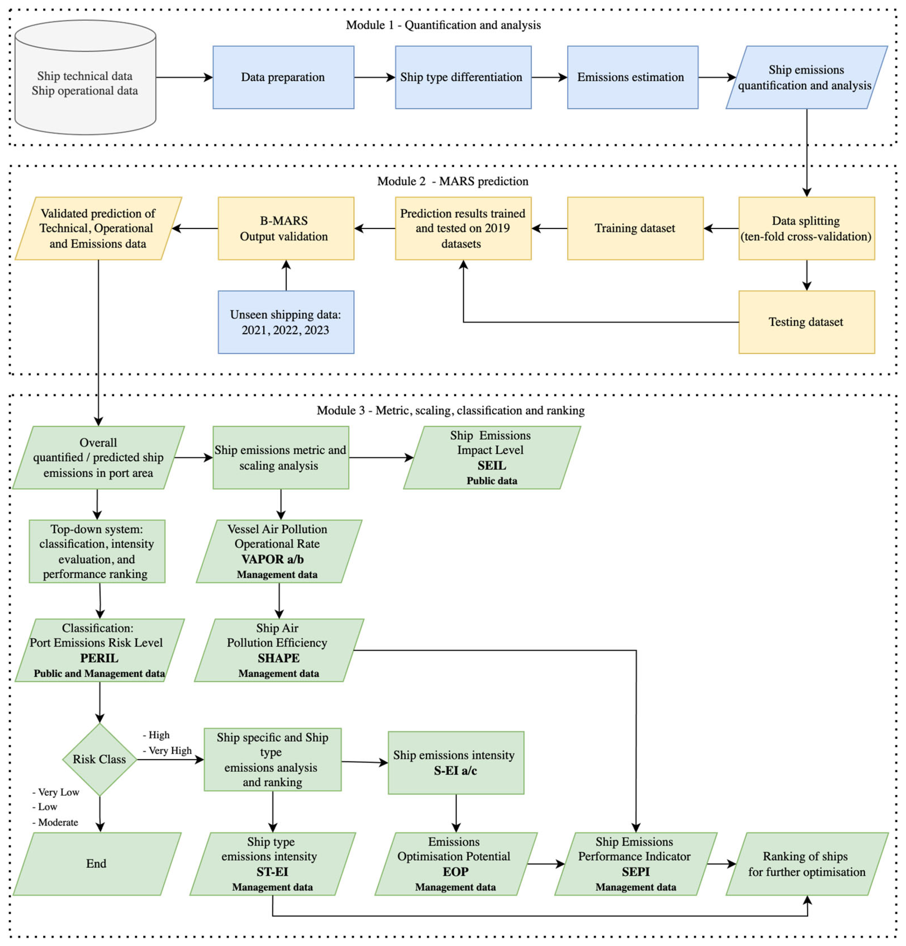
To perform the entire process, the model consists of three complex and interconnected modules, depicted in Figure 1. In the primary module for quantifying and analysing emissions, the collected technical and movement data were initially prepared with the aim of defining the voyage trajectories of each port arrival, stay, and departure for individual ships. These voyage datasets along with specific differentiation of ship types, enabled not only a high-density estimation of the air pollutants released by the individual ships together with various analytical results but also provided a basis for the extension of the model’s forecasting capabilities. Therefore, in the second component, machine learning algorithms were applied to the previously processed extensive technical and operational data to create a predictive module. Since the respective voyage trajectories of the individual ships represent complex data clusters that contain important factors influencing emission production, a Multivariable Adaptive Regression Spline (MARS) approach was adopted in this research to determine the effects of included factors and predict the emission quantities released in different scenarios. To evaluate the performance of the predictive module, ten runs of k-fold cross-validation were performed, with additional validation by comparing the predicted and actual results based on unseen data. The final component of the model is based on the data generated by the two previous modules and includes methods for assessing the emission intensity of ships, operational efficiency, and the temporal risk of air pollution. This has been achieved through the integration of novel metrics, scaling and risk classification, and ranking approaches, resulting in a transparent, comparable, and efficient overview of ship-based air pollution impact in port areas. Since the system does not only focus on carbon pollution but also includes the leading GHGs and APSs, it was able to calculate and evaluate the risk of shipping emissions for CO₂ and CH₄ as GHGs and SOx, NOx, PM10, PM2.5, NMVOC, and CO as APSs for each ship, a group of ships and an entire port area.

Given that the basic components of the model are derived from universal characteristics that significantly influence emissions production, the model is not limited to a single case study but can be applied to different ports. In addition, the modular structure of the model facilitates the integration of new insights and other relevant aspects of port-related shipping emissions, thereby improving the quality and scope of the final output. It is important to emphasise that the algorithms embedded in the PrE-PARE model and the data handling were produced using the software package RStudio 2023.09.1+494.

2.1. Emissions Estimation and Analysis Module

As stated, this paper builds on earlier work by the authors, particularly a systematic review and an article on an analytical model for estimating ship-related emissions in port areas [33,37]. The model presented in those studies served as the initial module, which was later adapted and integrated with novel predictive, risk evaluation, and metrics modules to form the PrE-PARE system. While the full details of this component and its methodologies are discussed at length in the cited papers, a summary is provided in this chapter to ensure a comprehensive understanding of the system introduced in this study [33].

The estimation and analysis module was therefore able to produce an inventory of ship emissions for large port areas, providing a detailed overview of technical, temporal, spatial, and operational aspects. To obtain the emission-related analytical results, the module integrates three main components [33]. In the initial phase, the technical and AIS datasets were pre-processed by applying conversion, cleansing, filtering, formatting, and merging methods. These steps were essential to configure the collected data so that it was suitable for calculating emissions through the module. The technical data recorded relate to gross tonnage (GT), length, breadth, year, main engine (MA) power, auxiliary engine (AE) power, engine type, engine speed, fuel type, speed at maximum continuous rating (MCR), and relevant emission mitigation technology. The activity data derived from AIS comprised 49,540,895 reference points, which were linked to the above-mentioned technical details of the corresponding ships via name, type, and MMSI number as identifiers [33].

This was followed by the differentiation of ship types and the estimation of emissions during the processing phase. To create categories of ships with similar technical characteristics, data on the function of the ship and details on ship dimensions, speed, and engines were considered. When certain ship types showed significant variations in some features (e.g., engine power), a probability distribution was applied to obtain more specific categories, eventually resulting in the identification of 11 ship types:

• Large Cruise Ships
• Ro-Ro Ferry
• Large Ro-Ro Ferry
• Small Cruise Ships
• Medium Cruise Ships
• High-Speed Crafts
• Excursion Ships
• Tug
• Pleasure Craft
• Fishing
• Sailing

Differentiating vessel types based on multiple characteristics improved the accuracy and efficiency of imputing missing data while providing the groundwork for the predictive capabilities of the next module [33].

In the second step of the processing phase, a bottom-up approach was applied, where reference points containing technical and operational data were combined into specific movement trajectories. Then, an energy-based method, which meets the requirements of the IPCC guidelines and is expressed in Equation (1), was used to calculate the total amount of air pollutants emitted during individual port calls for each ship [34]. Since speed alterations during port approaches lead to a change in energy output and, consequently, emission production, three operating modes (cruising, manoeuvring, and hoteling) with the time spent in them were determined for each trajectory [44]. This was done by estimating the workload of propulsion engines, known as load factor (LF), using the propeller law method expressed in Equation (2) [44]. As the cruising mode is identified by engine loads above 20% and manoeuvring is defined with LF values that are lower, hoteling operation is considered when the ships have switched their ME off and only use the generators while at berth or at anchor [27]. Subsequently, calculations were performed to estimate the quantities of greenhouse gases and air pollutants emitted by all vessels documented in the AIS database for the year 2019 within the study region.

Lastly, the output data was stored and handled with the goal of producing spatial and temporal visualisations of shipping emissions, as well as a detailed overview of various technical and operational aspects [37].

E = (P_ME × LF × EF_ME + P_AE × LF × EF_AE) × T × CF

(1)

where:

E: emissions quantity by mode for each ship call—in grams (g);

P_ME/_AE: total power of main engines/auxiliary engines—kilowatts (kW);

LF: load factor expressed as actual engine work output—as a percentage of engine power (%);

EF_ME/_AE: emission factors of different pollutants in regard to engine function,

engine type, fuel type, and installation year—in grams per kilowatt hour (g/kWh);

T: time spent in a certain movement activity—in hours (h);

CF: correction factor for emission reduction technologies—constant.

LF = (S_A/S_M)³

(2)

where:

S_A: actual speed of the ship—in knots (kt);

S_M: speed of the ship at MCR—in knots (kt)

2.2. Predictive Module

Since the first module already prepared detailed emissions-related data, it was possible to develop a predictive algorithm as the second component of the PrE-PARE model. However, as the production of different APSs and GHGs from marine engines is influenced by a variety of factors that interact with each other, the prediction of emissions cannot be determined by linear functions. The relationships between predictor variables, such as engine power, type and speed, fuel type, actual speed, energy output, and time in the different operating modes, and the released emissions are non-linear. In addition, the values of the parameters and their interactions vary between the ship types and individual ships. To overcome the complexity of predicting ship-related emissions, the MARS method was adopted in this research.

2.2.1. Multivariate Adaptive Regression Splines (MARS)

MARS is a nonparametric, piecewise regression technique applicable in the modelling and analysis of complex, nonlinear relationships between multiple dependent and independent variables [45]. To examine the interactions and capture nonlinearity, this method automatically creates piecewise polynomials that characterise the data [46]. These polynomials, referred to as splines, are basis functions inside the MARS model, and prediction is made by summing the weighted output of all the basis functions in the model [47]. Simple BFs involve a single variable (x) and come in pairs of the form (x − t) + and (t − x) +, where t is the knot, (x − t) + = (x − t) if x > t, and 0 otherwise; and (t − x) + = (t − x) if x < t, and 0 otherwise [47]. The modelling process has two main segments: the forward stage, which has the same idea as forward stepwise regression, and the backward (pruning) stage, r where the model is improved and validated [45,46,47]. The forward stage starts by including the constant mean of the target variable (intercept). This allows for determining the breakpoints or knots for each predictor variable. Between each point, a fitting basis function is added. This process is being done iteratively until the threshold is reached [45,46,47]. Once the full set of features has been created, the algorithm sequentially removes individual features that do not contribute significantly to the model equation to avoid overfitting [46,47]. This “pruning” procedure assesses each predictor variable and estimates the error rate aiming to eliminate basis functions with the least contribution [46,47]. This procedure is applied automatically through the Generalised Cross Validation (GCV) technique [45]. The GCV can be expressed as follows (3) [47]:

$$\mathrm{GCV}\left(\mathrm{M}\right) ={\displaystyle \frac{\frac{1}{\mathrm{n}}{\sum }_{\mathrm{i}=1}^{\mathrm{n}}({\mathrm{y}}_{\mathrm{i}}-{\widehat{\mathrm{f}}}_{\mathrm{M}}{\left({\mathrm{x}}_{\mathrm{i}}\right)}^2)}{{(1-\mathrm{C}(\mathrm{M})/\mathrm{n})}^2}}$$

(3)

where the denominator is a complexity function, and C(M) is defined as C(M) = (M + 1) + dM, of which C(M) is the number of parameters being fit and d represents a cost for each basis function optimization and is a smoothing parameter of the procedure [47]. Larger values for d will lead to fewer knots being placed and thereby smoother function estimates [45].

With the aim of obtaining more accurate results for the prediction of ship emissions, standard MARS and Boosting MARS (B-MARS) methods, with and without log normalisation, were applied in this research to historical data processed by a previous module. This approach resulted in four distinct predictive models. Their performance was assessed and compared to determine their accuracy and reliability. To ensure an unbiased selection of data and evaluate the models, k-fold cross-validation was used during the hyperparameter tuning process for MARS models where a ten-fold approach was applied. The data used for testing and training, with validation results averaged over ten runs, includes technical details and operational data derived from the AIS of ships that called at the port in 2019.

2.2.2. Prediction Performance Validation Metrics

To evaluate the performance of the above MARS models, the Root Mean Squared Error (RMSE), Mean Absolute Error (MAE), and Coefficient of Determination (R²), presented in Equations (4)–(6), were applied in this research [46]. These metrics assess the accuracy of the predictions by quantifying the errors between predicted and actual values [48]. The R2 score measures the proportion of variance in the dependent variable that the model explains [48]. Its value ranges from 0 to 1, with a value closer to 1 indicating a stronger relationship between variables and better predictive accuracy [49]. The RMSE calculates the square root of the mean of the squared differences between predicted and actual values [46]. As the errors are squared before averaging, the RMSE is more sensitive to larger errors and directly relates to Euclidean distance [46]. A lower value indicates better performance. MAE is used to measure the average absolute difference between predicted and observed values [45,48]. Unlike RMSE, this method treats all errors equally without squaring them, making it less sensitive to larger deviations [48]. A low MAE indicates higher prediction accuracy.

Although the above criteria are commonly used to evaluate the prediction of the models, additional validation was performed in this research by including unseen shipping data from 2021, 2022, and 2023. These datasets were first used to calculate ship emissions, and the results were then compared to those predicted by the module relying on historical data from 2019, aiming to gain a clear insight into its forecasting capabilities.

$${\mathrm{R}}^2=1 {\displaystyle \frac{{\sum }_{\mathrm{i}=1}^{\mathrm{n}}{(\mathrm{X}}_{\mathrm{i}}-{ \mathrm{Y}}_{\mathrm{i}}{)}^2}{({\sum }_{\mathrm{i}=1}^{\mathrm{n}}(\stackrel{\mathrm{-}}{\mathrm{Y}}-{ \mathrm{Y}}_{\mathrm{i}}{)}^2}}$$

(4)

$$\mathrm{MAE}={\displaystyle \frac{1}{\mathrm{n}}}\sum _{\mathrm{i}=1}^{\mathrm{n}}\left|{\mathrm{X}}_{\mathrm{i}}-{\mathrm{Y}}_{\mathrm{i}}\right|$$

(5)

$$\mathrm{RMSE} =\sqrt{{\displaystyle \frac{{\sum }_{\mathrm{i}=1}^{\mathrm{n}}{(\mathrm{X}}_{\mathrm{i}}-{\mathrm{Y}}_{\mathrm{i}}{)}^2}{\mathrm{n}}}}$$

(6)

where X_i is the predicted ith value, Y_i element is the actual ith value, and n stands for the number of samples [48,50].

2.3. Ship Emissions Metric, Scaling, Classification, and Ranking Module

As outlined in the introduction, the IMO has implemented various measures to regulate and assess the carbon efficiency of ships, which have become basic tools in the global effort to reduce CO₂ emissions from the shipping industry. However, significant methodological limitations have been identified in mentioned measures. These constraints are particularly evident in their narrow focus on CO₂, which disregards other exhaust gases, and can lead to the overall environmental impact of ship emissions being overlooked, especially in urbanised port areas. Additionally, the carbon intensity calculations exclude the hoteling phase, leading to inconsistent results that may not accurately reflect a ship’s total emissions profile. Adding to these issues, the measures do not fully incorporate operational data of the ships, which means that valuable insights into more realistic performance and efficiency are missing. Lastly, current imposed air pollution limitations are generally considered insufficient to address the full scope of the industry’s environmental impact, emphasising the need for more comprehensive and differentiated approaches to assessing and regulating the sector’s environmental footprint.

Consequently, the final objective of this research was to determine the air pollution impact and efficiency of ships while also providing a risk evaluation of temporal emission levels for individual ships, groups of ships, and the entire port area. This was achieved in the third module, where novel metric, scaling, classification, and ranking methods were applied to the outputs of the first and second modules.

2.3.1. Novel Metric and Scaling Systems for Standardised Measurement and Transparent Overview of the Emission Efficiency and Impact of Ships

To establish a systematic approach for assessing the efficiency and impact of air pollution from individual ships while ensuring standardised measurement, the operational output of maritime transport must first be defined and weighted. Given that the primary objective of the shipping industry is to provide safe and efficient transport, emissions should be evaluated in relation to this goal.

Therefore, Operational Efficiency (OE) should be defined as the ability of a ship to complete a voyage on schedule with minimal energy consumption per unit of time, as represented in Equation (7). In the context of the port approach, a voyage includes arrival, stay, and departure, encompassing cruising, manoeuvring, and hoteling as three operational modes, ensuring a comprehensive assessment of the vessel’s operational profile. By integrating the time required to reach the expected EO with a ship’s capacity for the intended operation and by comparing it against the emissions generated during the voyage, it becomes possible to determine the Vessel Air Pollution Operational Rate (VAPOR) for each mode, as defined in Equation (8). Unlike the metric system proposed by the IMO, the VAPOR considers available operational data and emissions over the entire voyage by evaluating air pollution in each mode (cruising, manoeuvring, and hoteling), separately giving the average hourly rate of exhaust production per work capacity. This allows for a standardised and detailed metric of emissions efficiency within specific operational phases. To ensure relevance, clarity, and comparability, the feature scaling technique is therefore applied. The calculated VAPOR (VAPOR c) for a specific ship is normalised against the baseline VAPOR (VAPOR b) of the corresponding ship type, revealing the Ship Air Pollution Efficiency (SHAPE), as depicted by Equation (9). The VAPOR b is calculated by relying on an extensive emissions-related database for each predefined ship-type group, which is classified in the first module. This enables SHAPE to indicate whether a ship is operating more or less efficiently compared to the expected performance of its category. It also provides an insight into the progress made in the emission efficiency of certain ships and groups over time.

In addition, a simplified and user-friendly metric system has been developed to make the contribution of specific ships to air pollution in ports more transparent to the general public. Therefore, the Ship Emissions Impact Level (SEIL) compares the emissions released by a certain ship during a voyage relative to the average emissions per voyage of a generic ship within a defined time window, as shown in Equation (10). This approach provides a clear and intuitive visualisation of a ship’s air pollution impact during an entire port visit, making it easier for the wider port community to assess and compare emission levels using a standardised emissions impact scale.

$$\mathrm{EO} \left(\mathrm{kWh}\right)=\sum _{\mathrm{C},\mathrm{M},\mathrm{H}}\mathrm{O}\mathrm{p}\mathrm{e}\mathrm{r}\mathrm{a}\mathrm{t}\mathrm{i}\mathrm{o}\mathrm{n}\mathrm{a}\mathrm{l} \mathrm{L}\mathrm{F} \left(\mathrm{k}\mathrm{W}\right) \times \mathrm{O}\mathrm{p}\mathrm{e}\mathrm{r}\mathrm{a}\mathrm{t}\mathrm{i}\mathrm{o}\mathrm{n}\mathrm{a}\mathrm{l} \mathrm{t}\mathrm{i}\mathrm{m}\mathrm{e} \left(\mathrm{h}\right)$$

(7)

$$\mathrm{VAPOR} ={\displaystyle \frac{\mathrm{E}\mathrm{m}\mathrm{i}\mathrm{s}\mathrm{s}\mathrm{i}\mathrm{o}\mathrm{n}\mathrm{s} \left(\mathrm{g}\right)}{\mathrm{W}\mathrm{o}\mathrm{r}\mathrm{k}\mathrm{c}\mathrm{a}\mathrm{p}\mathrm{a}\mathrm{c}\mathrm{i}\mathrm{t}\mathrm{y} \mathrm{\ast } \mathrm{O}\mathrm{p}\mathrm{e}\mathrm{r}\mathrm{a}\mathrm{t}\mathrm{i}\mathrm{o}\mathrm{n}\mathrm{a}\mathrm{l}\mathrm{t}\mathrm{i}\mathrm{m}\mathrm{e} \left(\mathrm{h}\right)}}$$

(8)

$$\mathit{SHAPE} ={\displaystyle \frac{\mathrm{V}\mathrm{A}\mathrm{P}\mathrm{O}\mathrm{R} \mathrm{c}}{\mathrm{V}\mathrm{A}\mathrm{P}\mathrm{O}\mathrm{R} \mathrm{b}}}$$

(9)

$$\mathit{SEIL} ={\displaystyle \frac{\mathrm{S}\mathrm{h}\mathrm{i}\mathrm{p} \mathrm{e}\mathrm{m}\mathrm{i}\mathrm{s}\mathrm{s}\mathrm{i}\mathrm{o}\mathrm{n}\mathrm{s} \mathrm{i}\mathrm{n} \mathrm{v}\mathrm{o}\mathrm{y}\mathrm{a}\mathrm{g}\mathrm{e} \left(\mathrm{k}\mathrm{g}\right)}{\mathrm{G}\mathrm{e}\mathrm{n}\mathrm{e}\mathrm{r}\mathrm{i}\mathrm{c} \mathrm{s}\mathrm{h}\mathrm{i}\mathrm{p} \mathrm{e}\mathrm{m}\mathrm{i}\mathrm{s}\mathrm{s}\mathrm{i}\mathrm{o}\mathrm{n}\mathrm{s} \mathrm{i}\mathrm{n} \mathrm{v}\mathrm{o}\mathrm{y}\mathrm{a}\mathrm{g}\mathrm{e} \left(\mathrm{k}\mathrm{g}\right)}}$$

(10)

2.3.2. Comprehensive Top-Down System for Classifying Air Pollution Risk in Ports, Evaluating Emission Intensity, and Performance Ranking of Ships

While emission estimation follows a bottom-up methodology, this system first evaluates the exhaust gases released in the entire port, then the relevant contributions from ship types, and finally the performance of specific vessels. This stepwise process allows for a structured assessment by first identifying the risk level of overall emissions in a relevant area, followed by determining the air pollution intensity for different ship types, and finally evaluating ship-specific indicators of emission performance. The potential for emission optimisation is calculated and combined with SHAPE. The aim of this three-stage procedure is to ensure a fair and data-driven framework for the control of ship-sourced air pollution in ports by providing an overview from both a macro and micro perspective.

To achieve this, the Port Emissions Risk Level (PERIL) classification algorithm is developed to determine the degree of severity of overall ship emissions in the entire port area for a specified period, as a first of three steps. The algorithm categorises emissions into five levels (Very Low, Low, Moderate, High, and Very High) by comparing the calculated emission rates with threshold values derived from the annual average and the standard deviation. This approach uses the average as a central reference point, allowing a clear and standardised classification of emission intensity based on statistical distribution rather than setting arbitrary thresholds. Upon determining the limit values, the system can automatically classify quantified shipping emissions. If the total emissions exceed the high-risk threshold, further analysis is conducted in a second step where the contribution of each ship group to total emissions is analysed.

This includes the application of the Ship Type Emission Intensity (ST-EI) assessment, which determines the degree of air pollution of each ship group by comparing their average emissions per voyage with the average emissions per voyage across all ship types in a given period, as shown in Equation (11). This method is used to create a relevant emissions contribution scale aimed at prioritising certain ship types for possible emissions improvement.

As a part of a final step, the Emission Optimisation Potential (EOP) is calculated for each ship by comparing its actual emissions per work capacity in each mode of voyage defined as the Ship Emission Intensity (S-EI), against a reference baseline, as depicted in Equation (12). The EOP is therefore used to determine the range of possible emission optimisation by displaying emission exceedances with values greater than 1 or improvement of operations in stated voyage with values lower than 1. The baseline values of individual ships represent the volume of emissions released typically per work capacity in each mode of voyage and are determined by relying on historical records from the database provided in the first module. If the database lacks the operational and air pollution profile of a ship (first port visit), the second module is used for predicting the emission quantities by relying on the technical and movement data of similar ships in the corresponding category.

Although the EOP exposes the performance of individual ships in terms of air pollution in each segment of a specified voyage, some vessels may already operate efficiently, leaving little room for further optimisation. Therefore, to ensure objective ranking of ships, the Ship Emissions Performance Indicator (SEPI) is applied, where emissions efficiency determined through SHAPE is combined with the EOP as a measure of the ship’s operational performance in a specific voyage, as displayed in Equation (13). By incorporating both factors, SEPI enables a fair emissions attribution and ranking, ensuring that the ships with the highest improvement potential are prioritised in the final step.

$$\mathit{ST}-\mathit{EI} ={\displaystyle \frac{E_{st} \times V_{tot}}{V_{st} \times E_{tot}}}$$

(11)

$$\mathit{EOP} ={\displaystyle \frac{\mathrm{S}-\mathrm{E}\mathrm{I} \mathrm{a}}{\mathrm{S}-\mathrm{E}\mathrm{I} \mathrm{b}}}$$

(12)

SEPI = SHAPE × EOP

(13)

where the following definitions apply:

ST-EI: ship type emission intensity—normalised value (dimensionless);

Est: total emissions for a specific ship type—in kilograms (kg);

Vst: number of voyages for that ship type—dimensionless value

Etot: total emissions for all ship types in the period—in kilograms (kg)

Vtot: total voyages for all ship types in the period—dimensionless value

EOP: emission optimisation potential—normalised value (dimensionless)

S-EI a/b: ship emission intensity actual/baseline—as emission mass in the entire voyage per unit of work capacity (kg/wcu)

2.4. Data

All the above methodologies integrated inside the PrE-PARE model were applied to the technical and activity data of the ships that visited the Port of Split in 2019, used here as a case study. The mentioned datasets, along with corresponding EFs and LFs, were preprocessed in the first module, as briefly explained in Section 2.1, creating an extensive database of emission-related inputs used throughout all three components of the PrE-PARE model.

Technical details of relevant ships were sourced from the Croatian Register of Shipping (CRS), the Croatian Integrated Maritime Information System (CIMIS), and relevant shipping company websites. The collected attributes include ship dimensions, work capacity, year built, ME and AE power, type and speed, fuel type, max speed at MCR, and emission reduction technologies, along with identifiers such as name, type, and MMSI number [33].

Since the AIS is used for sharing timely information on ship characteristics and their movements between other vessels and the shore to improve navigational safety, its recorded data is also often applied for estimating emissions [30,38,51,52]. Therefore, the position of the ship, course and speed over ground (COG, SOG), with corresponding timestamps, along with the name and MMSI number of specific ships as identifiers were applied in this research. For collecting mentioned datasets, the AIS station of the Faculty of Maritime Studies in Split was employed. However, as AIS transmits messages in the National Marine Electronics Association (NMEA) sentence format, which is unrecognisable to RStudio software, a specific Python script was developed and integrated into the first module to convert the ‘raw’ data from AIS into a readable CSV format [33]. In the earlier mentioned preprocessing stage, erroneous and non-ship entries were then removed, resulting in 49,540,895 ship records from 2019. These were used for emission estimation in the initial module, but also for testing and training in the predictive module. The same procedure was applied to acquire an additional 15,930,840 AIS reference points of ships visiting the same port during different periods in 2021, 2022, and 2023. These datasets represented unseen data used for extended validation of outputs produced by the second module.

These AIS reference points were then connected with technical data of particular ships via respective identifiers, finally creating individual trajectories for each port visit. This process enabled the identification of operating modes with corresponding temporal and spatial characteristics in each recorded voyage by estimating the energy output of ME through the propeller law method [44]. The LFs for AE were taken from relevant studies as constant values [31,35,44]. Since all emission-related technical and activity details were identified and connected into a single database, the EFs could be determined as the final and most complex dataset required for estimating and evaluating ship emissions by applying the relevant methodologies described in the 3rd and 4th IMO GHG Study and the San Pedro Bay Ports Report [3,44,53]. The types of Efs, along with the elements for identifying them, are presented in

Table 1. Engine details, modes of operation, and types of EFs incorporated in the model.

Elements for Determination and Types of EFs
Engine Function	Engine Type	Engine Speed (rpm)	Fuel Type	Mode & LF		GHG EFs	APS EFs
ME	D	SS D < 300	MDO/MGO	C	LF = > 20%	CO2	SOx
AE	GTU	MS D 300–900	HFO	M	LF < 20%	CH4	NOx
	STU	HS D > 900	LNG	H	LF = < 2%		PM 10, 2.5
	DF						NMVOC
	D-E						CO

[33].

Within Table 1, D stands for diesel engine, GTU for gas turbine, STU for steam turbine, DF for dual fuel engine, D-E for diesel-electric engine, SS/MS/HS D for slow-/medium-/high-speed diesel engine, HFO for heavy fuel oil MDO/MGO for marine diesel/gas oil, and LNG for liquified natural gas [33].

3. Results

The integration of technical details with activity data within the PrE-PARE model enabled the determination of operating modes and EFs for each of the 65,471,735 AIS reference points. These complex emission-related datasets were then combined into individual voyage tracks for each ship that called at the port, creating a foundation for modelling, predicting, and evaluating ship emissions in large port areas. Therefore, the model has recognised 48,256 voyages to the passenger basin of the Port of Split in 2019 and in different periods of 2021, 2022, and 2023. However, it is important to emphasize that 2019 was used as the base year in this research, so the datasets from this year were used for defining reference points, and records from other periods served for validation. The recorded number of visits closely matched port traffic data, showing an average deviation of only 3% across all ship types, except for pleasure crafts, excursion, and sailing ships, which lacked consistent arrival figures in the different sources. This discrepancy is largely due to their irregular schedules, often resulting in underreported AIS data. In addition, the 3% deviation partly reflects the ability of AIS to capture even minor vessel movements, offering higher quality input for accurate emissions estimation compared to standard port statistics. The share of port calls between ship types is illustrated in Figure 2.

Of all the ships surveyed, the most frequently installed engine type is MS D (78%), followed by HS D (22%) and LS D (3%). The share of engine types other than D is below 1%, so their influence on overall emissions is limited. Given the engine specifications and the enforcement of the EU Sulphur Directive, it is assumed that the entire fleet operates on MDO/MGO with a maximum sulphur content of 0.1% for the duration of each voyage [33].

3.1. First Module—Emissions Estimation and Analysis

As already mentioned, the first module was based on the analytical model presented in the earlier research created by the authors of this paper. Thus, an overview of various detailed technical, temporal, spatial, and operational aspects of ship emissions was presented within an inventory of combustion gases released in the area relevant to the Port of Split—City port basin for 2019 [33]. Apart from an examination of monthly fluctuations relative to the annual average, the analysis was focused on different elements of annual emissions. This approach, standard for emission inventories, reveals only general insights, as emission levels and their distribution between ships change with intervals considered. To enable detailed analysis and a comprehensive evaluation of the risk and impact of emissions, the production of air pollution from marine engines should therefore be assessed over shorter timeframes. Given that a strong correlation was found between high emission levels and intensive seasonal traffic, a further and thorough examination of emissions at peak times should be considered.

That is why, the first module that combines energy-based method with bottom-up logic was used in this research to additionaly analyse the fluctuation of daily emissions in the baseline year. The graph of daily emission totals in Figure 3, represented by the blue line, confirms the seasonal trend but also shows considerable differences in day-to-day air pollutant levels released, not only between summer and winter periods but also within the same months. The magnitude of the emission spikes becomes even more apparent when compared against the annual average of 120,164 kg (kg), marked by the yellow line, with emissions on some days being more than twice as high as the mean. Given the evident daily variability of ship emissions, further analysis was conducted for a specific day in July, as this month was identified as the most critical.

Table 2. Emission totals in kg for the Port of Split passenger basin on 2 July 2019, quantified by the first module.

Ship Type	GHG		AP						Ship Type Totals
	CO2	CH4	SOx	NOx	PM10	PM2.5	NMVOC	CO
Large Cruise Ships	116,161.249	2.133	68.801	2174.880	39.936	36.741	94.975	9.674	118,588.391
Ro-Ro Ferry	63,221.461	1.102	37.466	885.589	20.553	18.908	54.663	48.716	64,288.459
Large Ro-Ro Ferry	39,378.559	0.758	23.300	733.636	13.703	12.607	36.573	3.364	40,202.501
Small Cruise Ships	35,969.292	0.642	21.315	655.656	12.220	11.242	27.581	5.751	36,703.699
Medium Cruise Ships	31,222.711	0.591	18.481	582.766	10.817	9.951	26.038	2.642	31,873.997
High-Speed Crafts	19,380.975	0.346	11.486	262.921	6.312	5.807	17.733	17.273	19,702.854
Excursion Ships	21,46.156	0.051	1.272	35.847	0.783	0.720	2.849	1.456	2189.134
Tug	14,60.308	0.028	0.865	18.785	0.480	0.442	1.324	1.413	1483.644
Pleasure Craft	1349.716	0.047	0.800	26.445	0.584	0.537	2.797	0.616	1381.542
Fishing	691.295	0.021	0.410	9.374	0.272	0.250	1.081	0.765	703.468
Sailing	94.409	0.002	0.056	2.026	0.035	0.032	0.117	0.038	96.715
Emission type Totals	311,076	6	184	5388	106	97	266	92	317,214

therefore presents the emissions quantified by the estimation and analysis module for the Port of Split passenger basin on 2 July 2019, the most emission-intensive day in the selected month. The table clearly shows that total ship emissions on that date were more than 2.5 times higher than the average for the base year, illustrating the severity of risk that air pollution poses to the urban environment in the short timespan. It is also evident that Large Cruise Ships are responsible for about 37% of the emissions on that day, releasing almost twice as much as Ro-Ro Ferries, the second largest contributor to pollution, and only 5% less than all other groups combined. This result contrasts with the annual totals and confirms the differences in the distribution of emissions over time.

By comparing the calculated exhaust gas values of the individual ship types with the corresponding number of voyages in the same period, expressed as a percentage in Figure 4, the disparity between the emissions released and the number of port calls for some groups becomes clear. For instance, High-speed crafts, which account for the largest share of voyages (37%), caused 6% of total emissions on a given day, while Large Cruise Ships produced 37% of total emissions from only 2% of visits. This example alone provides additional insight into the disproportionate contribution, supporting the need for a thorough analysis of the conditions that cause greater production of on-board exhaust gases.

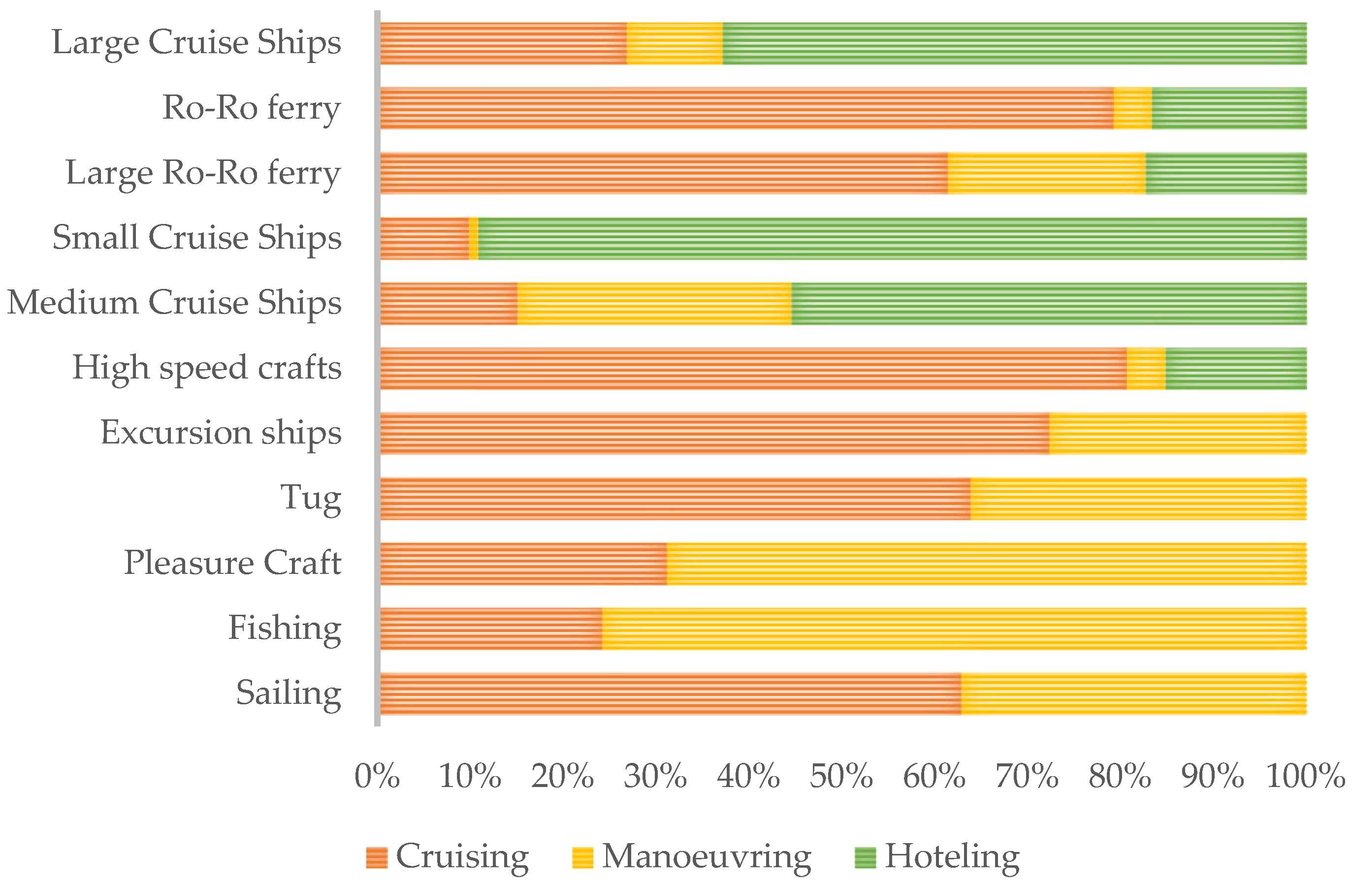
In this context, the first module was also used to examine the operational and spatial aspects of the emissions released on the selected day. Therefore, the distribution of emissions across operational modes was found to be 43%, 12%, and 46% during cruising, manoeuvring, and hoteling, respectively. These values deviate notably from the annual averages, highlighting temporal variations in emission patterns and confirming the differences in the generation of air pollutants between ship types in the diverse operational modes, as illustrated in Figure 5. As can be seen, all types of cruise ships released most of the emissions in the hoteling phase, fishing and pleasure crafts while manoeuvring, and all others through cruising mode.

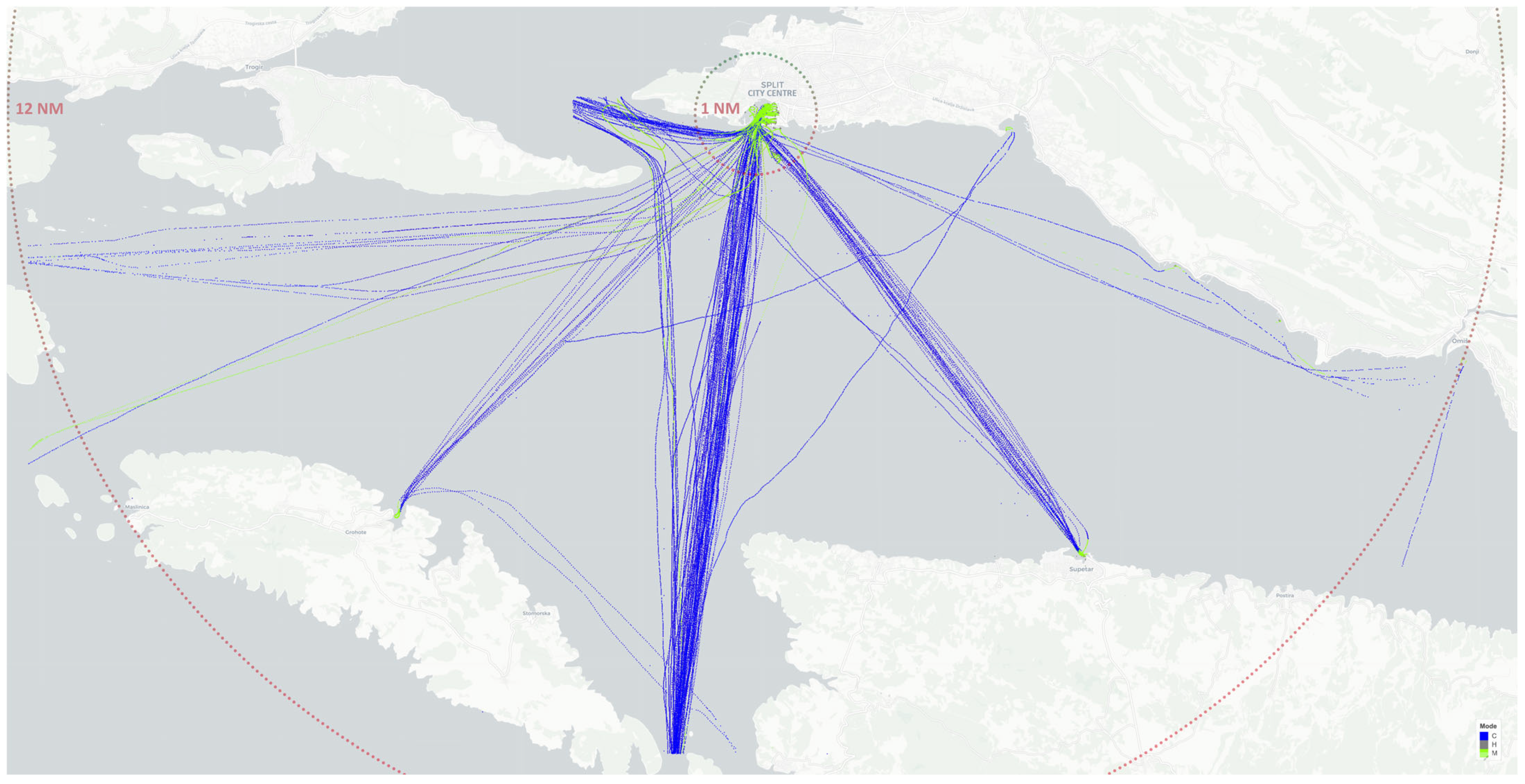
Since the identified activities and their corresponding emissions occur in distinct zones within the study area, a detailed map of the emission dispersion points was generated and is presented in Figure 6 to illustrate the spatial distribution of air pollution. An analysis of the emission release locations, categorised by operating modes within individual voyages, revealed that almost all air pollutants were released within a 12 nautical miles (NM) radius around the city centre of Split. Notably, emissions from hoteling and manoeuvring operations, comprising 58% of the day’s total, occurred only 0.5 NM from the urban area, highlighting their impact on the local atmosphere. This finding is especially relevant for APSs, which pose a direct threat to human health.

The development of a high-density map correlating emission dispersion points with operating modes provided a detailed overview of ship-based air pollution patterns in the port area. However, as shown in Figure 4, ships often operate differently, which directly affects emission output. Furthermore, the composition and workflow of the fleet involved changes within the timeframe examined, meaning that even reports based on large datasets only reflect conditions specific to the examined period. In order to achieve a comprehensive evaluation of ship emissions, machine learning techniques must therefore first be applied to provide relevant predictions of emissions under different scenarios on the basis of all the features analysed.

3.2. Second Module—Emissions Prediction Based on MARS Approach

In the second module, different MARS methods were applied to extensive emission-related datasets preprocessed and structured in the previous component, aiming to achieve more accurate and reliable predictive outputs. Specifically, standard MARS and B-MARS, both with and without log normalisation, were used on technical and 49,540,895 AIS records of ships that visited the Port of Split during the base year 2019.

As previously described, in each MARS model, a ten-fold cross-validation was implemented, where data was partitioned into ten equal subsets. Each of the ten iterations interchangeably included different 90% of the datasets in the training fold and 10% in the testing fold, ensuring randomised and unbiased selection of inputs. To obtain a clear, and data-driven evaluation of the outputs produced by each MARS model, RMSE, MAE, and R² were calculated as key performance metrics and compared across all runs. Given the operational and technical differences between ships, each MARS variant was validated separately for distinct ship categories and operational phases.

Table 3. Performance metric comparison of ship emissions predictive models.

Ship Type	Mode	Metric	MARS Models
			Log-Scale MARS	Original MARS	MARS Without Log	Log-Scale B-MARS	Original B-MARS	B-MARS Without Log
Cruise Ships	C	RMSE	0.094	370,984.728 g	587,208.1 g	0.397	294,2934 g	566,174.7 g
		R2	0.997	0.996	0.990	0.920	0.74194	0.99269
		MAE	0.071	214,953.697 g	420,379 g	0.156	871,928 g	360,756.3 g
	M	RMSE	0.190	535,904 g	844,628 g	0.130	384,456 g	872,822 g
		R2	0.993	0.993	0.990	0.997	0.9977	0.984
		MAE	0.135	310,311 g	435,491 g	0.097	208,845 g	451,754 g
	H	RMSE	0.088	1,300,580 g	333,946.000 g	0.090	1,437,849 g	290,938 g
		R2	0.997	0.995	1.000	0.997	0.9934	0.999
		MAE	0.056	733,883.000 g	187,609.000 g	0.058	749,500 g	178,251 g
Ro-Ro Ferries	C	RMSE	0.070	74,100 g	100,525 g	0.062	78,208 g	80,749 g
		R2	0.989	0.997	0.994	0.991	0.9963	0.9626
		MAE	0.025	41,076 g	54,154 g	0.027	46,851 g	472,078 g
	M	RMSE	0.130	45,728 g	32,810 g	0.126	38,581 g	27,135 g
		R2	0.991	0.910	0.955	0.991	0.9377	0.9694
		MAE	0.071	6989 g	9360 g	0.061	5542 g	8057 g
	H	RMSE	0.634	130,894.91 g	104,916 g	0.641	136,666 g	73,625 g
		R2	0.852	0.997	0.996	0.832	0.9962	0.998
		MAE	0.176	41,719.50 g	37,042 g	0.270	41,021 g	17,496 g

presents the average key performance metrics for all categories of Cruise Ships and Ro-Ro Ferries, selected as representative case studies due to their contribution of over 90% of the total recorded emissions. These examples effectively illustrate the predictive capability of the developed models across dominant ship types and operational scenarios.

The performance metrics of all four predictive models include RMSE, MAE, and R² values for all categories of Cruise Ships and Ro-Ro Ferries across three operational modes. Models trained with log-normalised emissions were evaluated in both logarithmic units (Log-Scale MARS and Log-Scale B-MARS) and their anti-logarithmic equivalents (Original MARS and Original B-MARS), resulting in some metrics being expressed in grammes to provide interpretable, real-world error values. On the other hand, metric results for the models trained and evaluated entirely on raw emission values (MARS and B-MARS without log) were shown only in grammes, as no normalisation was applied.

Overall, log-normalised models generally performed better when handling skewed data, but performance varied by ship type and mode. Notably, B-MARS without log transformation achieved the lowest MAE and RMSE values in certain cases (e.g., Ro-Ro ships in mode M with an MAE of 17,459 g), suggesting that models based on raw values can outperform log-transformed ones when the data distribution is more balanced. These results showed that the most effective approach depends not only on the algorithm but also on the nature of the emission data in different operational contexts.

However, since the B-MARS model trained without the log transformation showed the most accurate prediction performance on average, it was implemented in the PrE-PARE system as the second module. Although the results generated by the chosen prediction module showed high accuracy, further validation was performed with unseen data. This was done to verify the module’s ability to accurately predict emissions in different scenarios with unknown (first visit) ships and unpredictable changes in the operation of the included vessels. Therefore, a total of 15,930,840 AIS reference points and the corresponding technical details of the ships calling at the port in different periods of 2021, 2022, and 2023 were applied as unseen data for the extended validation of the results produced by the second module.

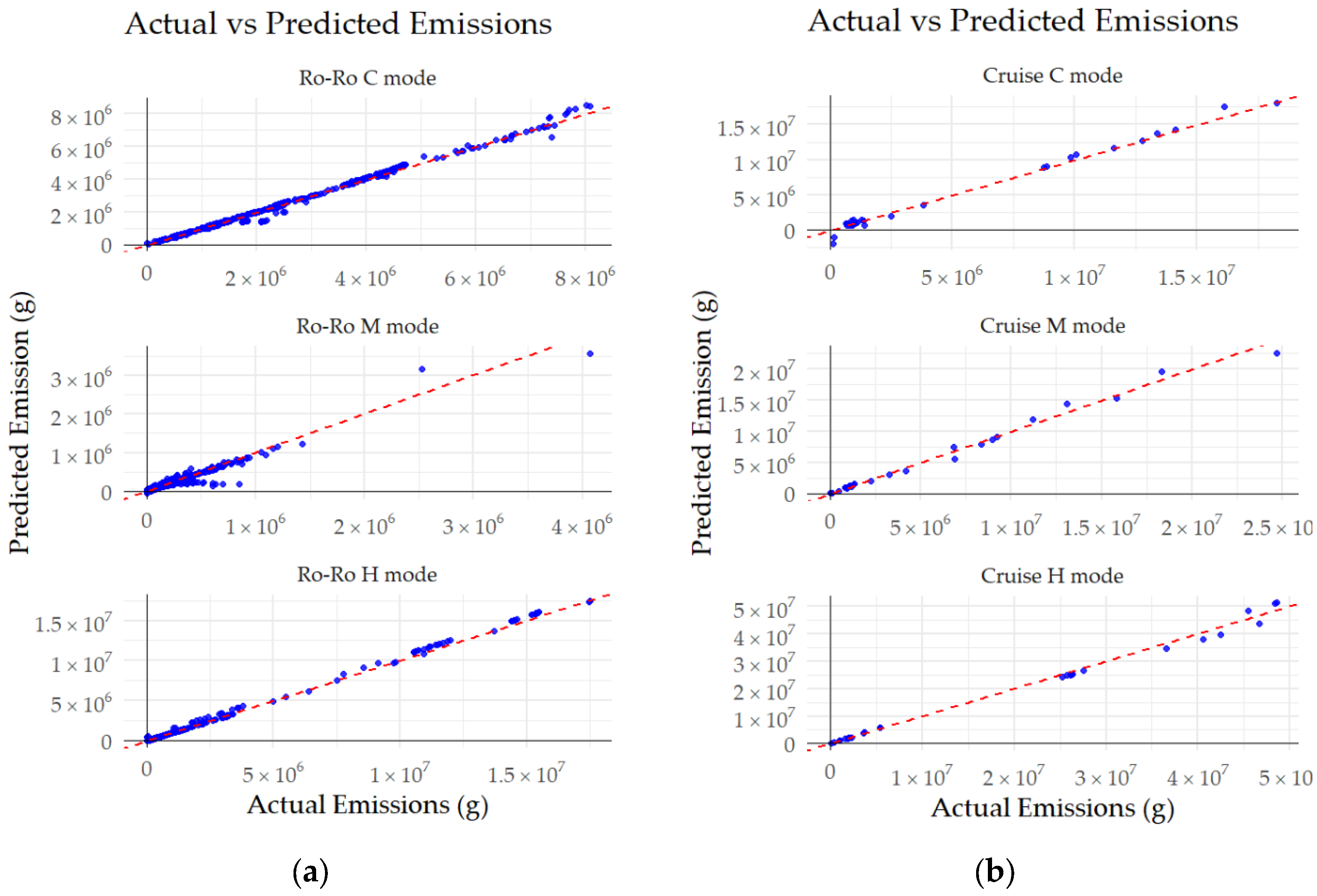
In this process, the non-log B-MARS module, trained on emission data from 2019, was used to predict emissions from Cruise Ships and Ro-Ro Ferries in all three modes. These were then compared with the actual levels released by the corresponding ship types during 2021, 2022, and 2023, as shown in Figure 7. The graphs display cruising, manoeuvring, and hoteling modes from top to bottom, with panels labelled (a) corresponding to Ro-Ro Ferries and those labelled (b) representing Cruise Ships. The blue dots in each scatter plot present emissions predicted by the module, while the actual emissions based on real data are illustrated by the red dotted line.

In all modes and for both ship types, the predictions closely match the reference line, indicating that the model generalises well beyond its original training dataset. The strongest alignment is observed in the cruising and hoteling modes, where the predictions show minimal deviation from the actual values. Even though some over or underestimation can be observed for outliers with high emissions, especially in manoeuvring and hoteling operations of Cruise Ships, the overall performance indicates that the B-MARS model trained on 2019 data is able to produce robust and accurate predictions of ship emissions in different scenarios and future trends.

3.3. Third Module—Ship Emissions Metric, Scaling, Classification, and Ranking Module

Although the second module demonstrated effective predictive performance for ship exhaust gasses even under new conditions, the modelled results always reflect the emission-related attributes of a specified period, as determined by analysing the outputs generated by the first module. Spatial, temporal, technical, and operational aspects vary with the intervals considered, which limits the broader interpretability and comparability of the results. Furthermore, the repeated generation, examination, and comparison of results is time-consuming and requires both computational and expert resources. Therefore, adopting a standardised system for evaluating air pollution risk in ports, ranking emission intensity, and assessing the potential for ship emission optimisation would be a more efficient and scalable solution. For this reason, novel methods integrated within the third module were applied to outputs produced by the analytical component of the PrE-PARE system.

3.3.1. Standardised and Interpretable Measurement of Ship Emissions Efficiency and Impact Based on Novel Metric and Scaling Methods

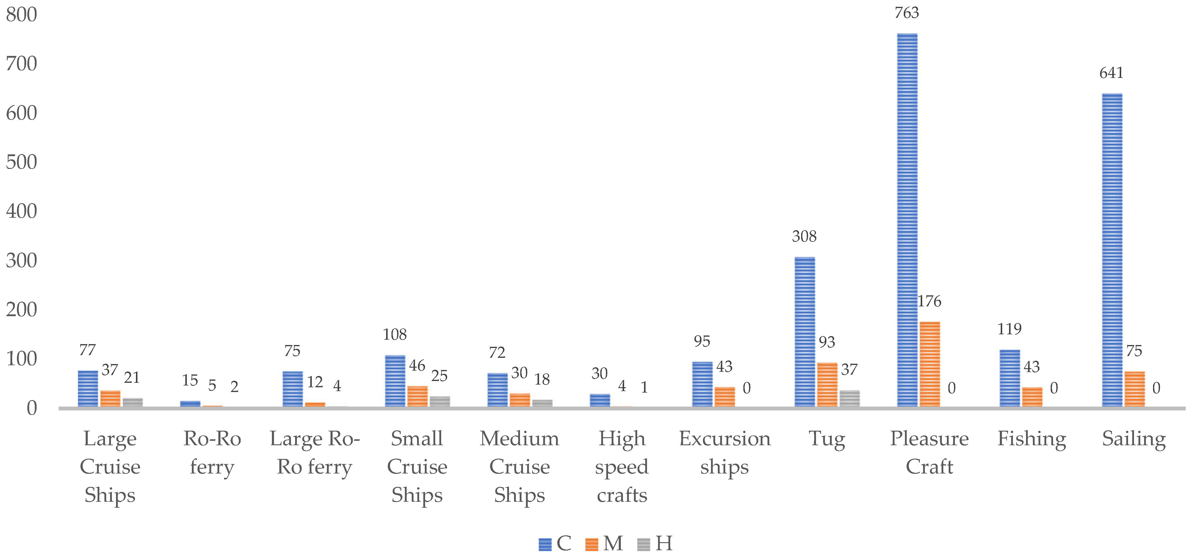
As a central method to universally determine the emission efficiency and performance of individual ships, VAPOR, a novel metric system, was established and applied in this research. Processed datasets of all ships recorded in 2019 were used to calculate the baseline VAPOR (VAPOR-b), which quantifies hourly emissions production in grammes (g) per unit of working capacity in different modes of operation. For all types of cruise ships, high-speed vessels, pleasure craft, sailing ships, and excursion vessels, the working capacity was defined based on passenger capacity. In the case of Ro-Ro Ferries, both passenger and vehicle capacity were considered. For tugboats, the bollard pull was used as a measure of working capacity, while for fishing vessels the net volume of cargo space was applied. These results were aggregated to derive the average VAPOR-b for each ship type, as illustrated in Figure 8, for APSs (SOx, NOx, PM10, PM2.5, NMVOC, and CO), representing emissions with local impact. It must be clarified that the maximum working capacity has been used as a static value, independent of the actual utilisation of the ships, to create a static reference point that can be compared with the actual emission production, optionally considering the actual workload of the individual ships. Furthermore, in the context of port visits, which include arrival, stay and departure, the mentioned capacities have been doubled for all vessels as they are able to embark/load and disembark/unload passengers/goods during a single voyage, as defined in this research. The exceptions are Tugs, as their working capacity is defined by the bollard pull, and Fishing Vessels, which use their capacity at sea and do not overturn goods in both directions. When comparing all three modes of operation, Pleasure Crafts exhibited the highest hourly rate of exhaust production per unit of work capacity, reaching 763 g in cruising mode. This highlights the correlation between small work capacity and relatively high-demand engines. In contrast, Ro-Ro Ferries, which are often equipped with similarly powerful engines but with large work capacity, demonstrated the overall lowest emission rates per working unit, despite being the largest annual polluters and the second in total emissions on the observed day. In addition, Sailing Ships showed a high emission rate of 640 g in cruise mode, due to the assumption of continuous engine usage; thus, the analysis in this study reflects the worst-case operational scenario for this ship type.

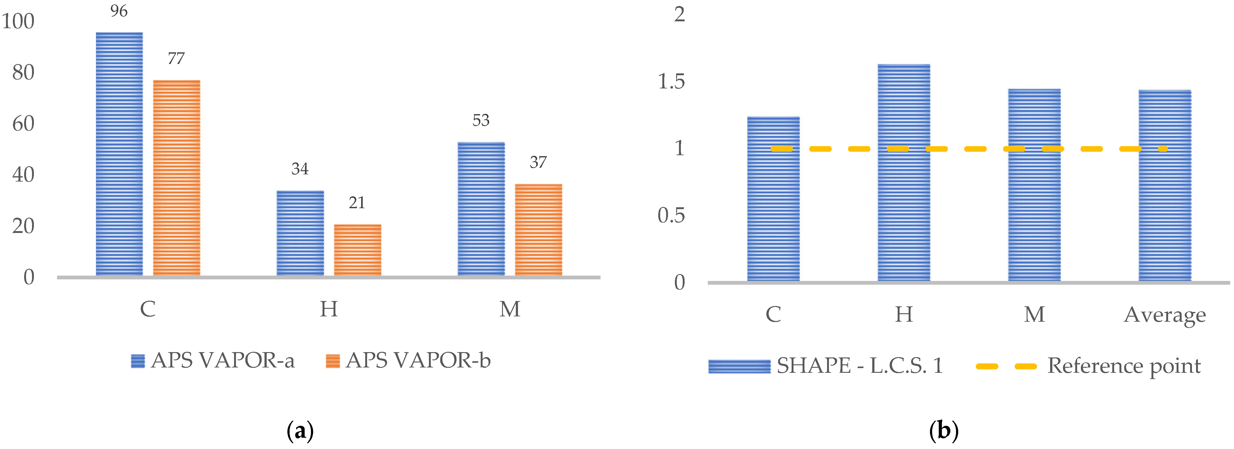
These baseline values were then applied in a scaling process, where they were compared to the actual VAPOR (VAPOR-a) calculated for vessels calling at the port on 2 July 2019. It is important to note that the work capacities used for calculating VAPOR-a were treated consistently with those applied to VAPOR-b. By correlating mentioned values, the SHAPE metric was derived for each operational mode of every ship recorded on the observed day. The SHAPE values greater than 1 indicate reduced emission efficiency (higher actual hourly emission rate per capacity), whereas values below 1 reflect better efficiency. Given that the Large Cruise Ships were recognised as the most significant contributors to emissions on the stated day, Figure 9 presents the APS results from both the metric and scaling perspectives for one representative vessel from this category. The left-hand panel (a) displays a comparison between the calculated VAPOR-a and the reference VAPOR-b across operational modes. For example, Large Cruise Ship 1 (L.C.S. 1) in the hoteling phase produced 13 g of APSs per unit of capacity more per hour than ships with similar characteristics. The right-hand panel (b) illustrates the corresponding SHAPE values, normalised against the baseline. The bars represent the ship’s actual efficiency, while the yellow dashed line indicates the reference point (SHAPE = 1). These results show that L.C.S. 1 was, on average, less efficient in all operating modes.

The application of VAPOR and SHAPE to the case of L.C.S. 1 clearly demonstrates the ability of these metrics to provide transparent and pragmatic insights. As can be seen in Figure 8, both the raw (VAPOR) and normalised (SHAPE) results are intuitively visualised across all operating modes, enabling easy identification of inefficiencies in this example. The standardised calculation method, which is based on available operating and emissions data, ensures that the results are not only objective but also directly comparable with ships of similar features. The simplicity of interpretation, particularly through the SHAPE values relative to the baseline, makes these metrics highly effective for communicating emissions performance, as they do not require extensive expert or computational resources. In addition, as the metric is based on available operational data, it provides more realistic results and can be used universally to monitor the emission efficiency of ships at an international level.

To complement the technical metrics with a more accessible perspective for the wider port community, the SEIL was applied to the analysed day. As a simplified and intuitive indicator, the SEIL expresses the total emissions released by each ship during its port visit relative to the emissions of a “generic” ship, whose value is derived by aggregating the total emissions and voyages of all ships recorded on that day. This allows a clear comparison of individual ship impacts on a standardised scale. As illustrated in Figure 10, SEIL provided a visual ranking of ships based on their emissions per voyage on a selected day, highlighting those that contribute more than average to air pollution in the port area. The introduction of this metric supports greater transparency and enables informed discussions on emissions accountability among port stakeholders and the general public.

The SEIL results clearly reveal the disproportionately high environmental impact of certain ships. In particular, Large Cruise Ship 1 emitted over 17 times more air pollutants than the average ship during a single voyage on the examined day. This straightforward contrast emphasises the magnitude of emissions caused by high-consumption ships. Furthermore, the results show that while Ro-Ro Ferries as a group make the second largest contribution to emissions, a typical Ro-Ro ferry would have to make approximately 23 separate voyages to match the emissions generated during a single port visit by the Large Cruise Ship 1. These results highlight the extent to which such ships contribute to local air pollution and emphasise the importance of differentiated emission management strategies in port operations.

3.3.2. Classification of Air Pollution Risk and Ranking of Ships Based on Emission Intensity, Optimisation Potential, and Performance in Port Areas

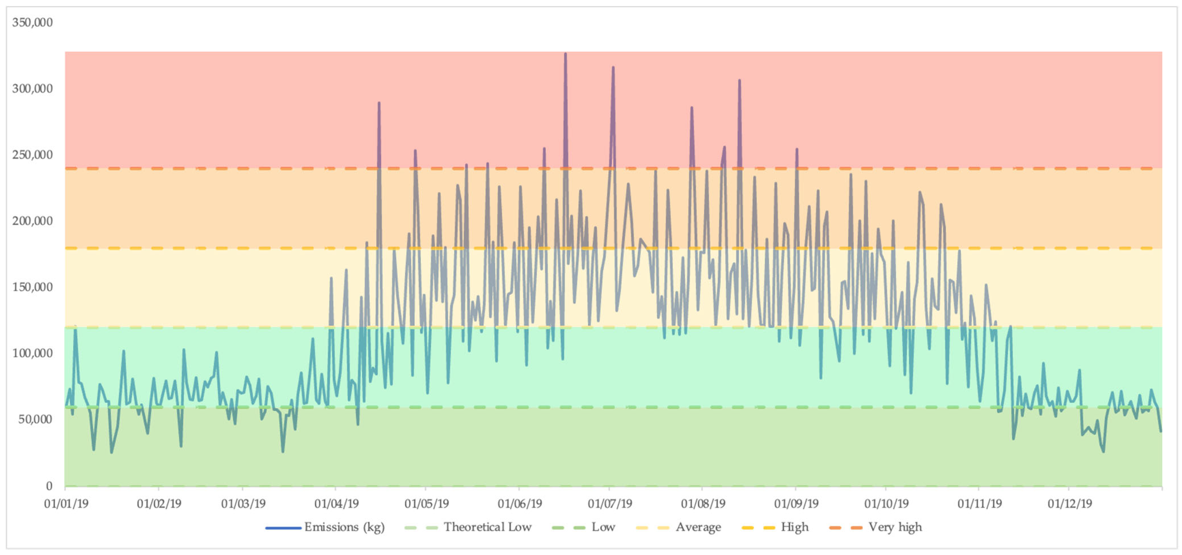
To effectively evaluate and manage ship emissions in the port areas, a top-down system for determining air pollution risk, intensity, and performance was developed and applied to real operational data. As the first part of a three-step process, the PERIL classification algorithm was implemented on daily emission totals quantified by the first module for the baseline year 2019. This approach, based on statistical distribution, segments daily emissions into five categories by using standard deviation and the mean value as central reference points. These categories are visualised in Figure 11, where thresholds are defined from the annual average of daily exhaust gases and their variability: Very Low (dark green) spans from 0 kg to 60,081 kg, Low (light green) from 60,081 kg to 120,163 kg, Moderate (yellow) from 120,163 kg to 180,246 kg, High (orange) from 180,246 kg to 240,327 kg, and Very High (red) includes all values above 240,327 kg.

Although the Moderate zone begins above the average, it encompasses values within one standard deviation and can thus be considered as a part of the statistically normal range. This classification methodology avoids arbitrary thresholds and supports meaningful distinction between typical and extreme emission events, enabling targeted emission control, particularly in the High and Very High categories. According to the PERIL classification, 13 out of 360 days were categorised as Very High risk and 50 as High risk, with these events distributed between April and November. This finding indicates that overall, only a minority of days have a significantly increased risk.

Due to total ship emissions reaching 317,214 kg on 2 July 2019, corresponding to 2.6 standard deviations above the annual mean, the day was clearly classified in the Very High risk category. This result prompted further analysis aiming to categorically identify the sources of high ship emissions.

To determine the distribution of emissions among the various ship groups, the ST-EI method was applied as the second step in the bottom-down approach. This measure compares the quantified emissions per voyage for each ship type with the overall average for the fleet during the analysed the period, thus highlighting categories with significant intensity.

As can be seen in Figure 12, Large Cruise Ships exhibited the highest APS intensity of all ship types on the observed day, indicating that they had the most significant impact per port call. This result served as the basis for further analysis of the individual vessels first within this group to assess their optimisation potential.

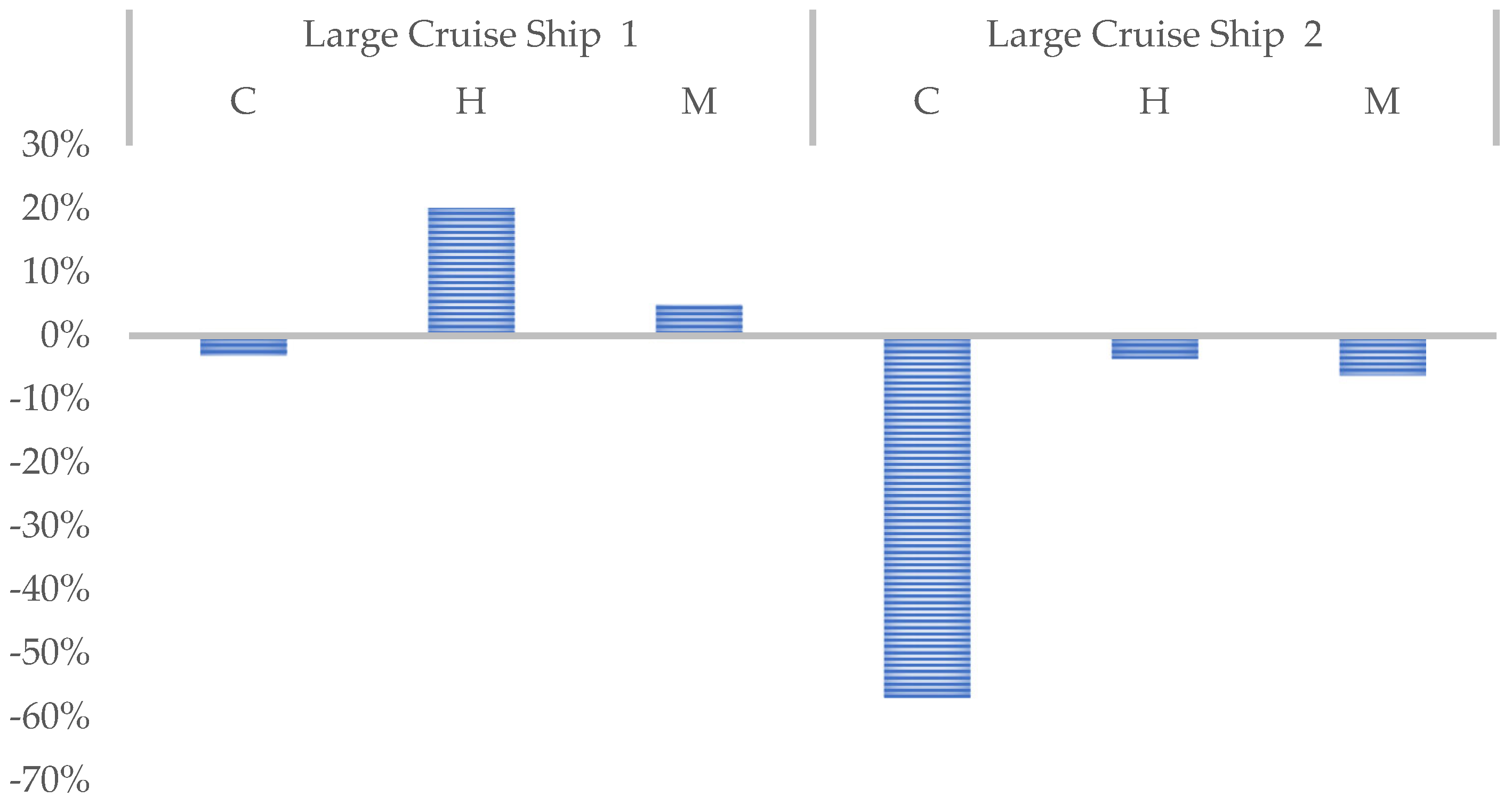
In the final stage of the process, the EOP was calculated to determine the quantity of emissions that could realistically be reduced. This was initially performed for the two ships that comprise the entire Large Cruise Ship category by comparing their actual emission per work capacity (S-EI a) through the entire voyage with their historical baseline (S-EI b), which reflects the average emissions released per work capacity during all previous port visits.

In contrast to VAPOR, which is a universal metric method that quantifies the hourly production of emissions per capacity, the S-EI used in the EOP focuses on the total emissions during a complete voyage. It integrates the total time spent in each mode and is thus sensitive to the temporal and spatial differences specific to the operational pattern of individual ships. Due to these variations, the S-EI cannot be used for a direct and clear comparison between ships. Instead, it enables intra-ship performance evaluation by comparing each voyage with the vessel’s own operational history.

As shown in Figure 13, Large Cruise Ship 2 exhibited lower-than-expected emissions in all voyage segments, indicating overall efficient operation. In contrast, Large Cruise Ship 1 demonstrated higher emission outputs in hoteling by 20% and by 5% higher in manoeuvring operations, while cruising was slightly below average, suggesting concrete potential for improvement. The EOP values were then combined with SHAPE, a metric that reflects the universal emissions efficiency of each ship, to calculate the Ship Emissions Performance Indicator (SEPI). By integrating emission efficiency and optimisation potential, SEPI enables a fair and balanced ranking of vessels.

In the end, all ships recorded on the analysed day were automatically categorised, first by ST-EI and then by SEPI, with the corresponding SHAPE and EOP values, as displayed in

Table 4. Ranking of the top ten ships in the Port of Split on 2 July 2019, based first on the ST-EI and then SEPI indicators for the entire voyage, including SHAPE and EOP values for each operating mode.

Ranking	Name	ST-EI	Mode	SHAPE	EOP	SEPI Voyage
1	Large Cruise Ship 1	16.26	C	1.24	0.97	1.56
			H	1.64	1.20
			M	1.45	1.05
2	Medium Cruise Ship 1	11.91	C	0.96	0.70	1.16
			H	1.17	0.95
			M	1.04	1.62
3	Ro-Ro Ferry 9	0.58	C	1.21	1.11	2.37
			H	1.20	3.37
			M	0.99	1.75
4	Ro-Ro Ferry 4	0.58	C	1.49	0.90	1.92
			H	1.61	0.67
			M	1.49	2.23
5	Ro-Ro Ferry 4	0.58	C	1.76	1.06	1.52
			H	1.61	0.11
			M	1.31	1.92
6	Ro-Ro Ferry 6	0.58	C	0.99	1.14	1.22
			H	0.76	2.10
			M	0.64	1.44
7	Tug 1	0.41	C	0.99	1.11	1.05
			M	2.16	0.47
8	High-Speed Craft 1	0.17	C	0.93	1.09	1.50
			M	0.85	2.35
9	High-Speed Craft 7	0.17	C	1.81	1.56	1.37
			H	1.18	1.07
			M	0.00	0.86
10	High-Speed Craft 8	0.17	C	1.02	0.18	1.30
			H	1.07	1.59
			M	1.05	1.93

for the top 10 ranked ships. This layered classification enables not only targeted emission control for the most intensive vessel types but also identifies specific vessels that should be prioritised for further optimisation interventions, ensuring a fair and data-driven basis for port emissions management.

4. Discussion

The results generated by the PrE-PARE model demonstrate that, by applying the methodologies integrated within its three modules to extensive technical and operational data, ship-sourced emissions in port areas can be effectively quantified, analysed, predicted, evaluated, and categorised in a clear, comparable, and standardised manner. Although each module can operate separately and produce function-specific outputs, their compatibility and shared reliance on structured shipping data support the control of port-related air pollution by simplifying the complex relations between the different aspects of ship emissions as a final outcome. As demonstrated in this and previous studies, technical, temporal, spatial, and operational factors vary in relation to the area and period considered, leading to inconsistencies in the interpretation of their influence on port-related air pollution. This variability complicates the analysis and prevents a meaningful comparison of the results in different contexts. The combination of novel metric, scaling, classification, and ranking methods with quantified emissions-related data, therefore, enabled an effective interpretation of the various implications crucial for analysing and managing ship emissions in ports throughout changing conditions. In practical terms, the PrE-PARE model provides tangible answers to critical management questions: What level of emissions should be considered high for a given port? Which ships perform efficiently in terms of emissions? Which vessels should be prioritised for operational optimisation?

The introduction of VAPOR and SHAPE as central metric methodologies addressed the need for a universal, data-driven measure of ship emission efficiency. In contrast to conventional regulatory indicators such as EEDI, EEXI, or CII, which are primarily based on theoretical design parameters and emissions per NM, and overlook time spent in port, VAPOR reflects hourly emissions per ship-specific unit of work capacity across all operational modes, including cruising, manoeuvring, and hoteling, by relying on available operational data. Moreover, while the referenced IMO indicators are limited to assessing CO₂ emissions, the metrics presented in this research encompass a broader range of air pollutants, offering a more comprehensive evaluation of a ship’s environmental footprint. Additionally, the application of SHAPE facilitates comparability by normalising and comparing calculated values against category-specific baselines, thereby enabling clear and consistent performance monitoring. The practicality of using the PrE-PARE metrics is demonstrated by comparing Ro-Ro Ferries and Large Cruise Ships, both of which contribute significantly to emissions in the Port of Split. While Large Cruise Ships were the dominant emitters on the analysed day, Ro-Ro Ferries accounted for the highest annual totals. However, across all operational modes, Ro-Ro Ferries emitted approximately 5 to 10 times less APSs than Large Cruise Ships on VAPOR-b. This contrast emphasises the value of applying standardised metrics that account for a ship’s work capacity and applying a consistent time unit, such as hourly output, allowing a meaningful assessment of performance for different ship types and timeframes in all operating modes.

Although VAPOR was applied within the port area in this study, its calculation is not spatially limited. The model can be extended to evaluate emissions along the entire voyage, allowing a continuous analysis from port to port on sea and ocean passages. This flexibility makes the model suitable not only for port management but also for regional policy development, transboundary environmental assessments, and global monitoring of the efficiency of specific ships and related groups. In addition to these metrics, the SEIL indicator further simplifies the interpretation of a ship’s air pollution during a single voyage, making the results accessible to experts and inclusive for the broader community.

To evaluate the risk of shipping emissions in different timeframes, the PERIL classification algorithm was developed and applied, where aggregated averages and standard deviations are used to objectively classify overall port emissions into categories ranging from Very Low to Very High. In the context of this research, the algorithm identified only 13 Very High and 50 High emission days for the Port of Split, unevenly distributed throughout 2019, highlighting the need for improved management of port activities, particularly during expected peak emission periods.

Following PERIL classification and continuing the top-down evaluation process, the ST-EI method was applied to identify and rank ship types based on their emission intensity relative to their operational activity. On the analysed day, Large Cruise Ships were recognised as the ship type with the highest emission intensity. This result directed the subsequent evaluation of all recorded vessels, starting with those within the high-impact group. The EOP and SEPI indicators were thus applied to determine both the emission performance and optimisation potential of individual ships. These indicators revealed clear distinctions in performance levels, enabling a fair and targeted ranking system that prioritises ships with the greatest room for improvement within relevant groups.

It is important to emphasise that, by combining a predictive module based on the B-MARS machine learning approach with other components of the model, the system extends beyond current conditions and enables the modelling, prediction, and evaluation of possible future pollution scenarios. This feature supports strategic planning and enhances port resilience against emerging operational and environmental challenges.

In this context, the modular structure of the PrE-PARE model ensures a high degree of flexibility, allowing for the possible integration of new methodological findings, regulatory requirements, or additional emission-related factors without changing the basic architecture and logic of the system. This adaptability also enables its application in different areas, maritime transport structures, and port operation contexts, regardless of size or local emission characteristics. At the same time, the outputs generated by the model remain consistent, comparable, and easy to interpret, as they are based on a relevant methodological foundation supported by extensive operational and technical data.

Ultimately, all the mentioned features support the future adaptation of the model as a decision-support system for the control of ship-based emissions in ports, as well as a framework for the introduction of air pollution tariffs within the broader context of integrated environmental management in seaports.

5. Conclusions

The PrE-PARE model presented in this research demonstrated the capacity to model, analyse, predict, and comprehensively evaluate port-related air pollution from ships by combining relevant methodologies with emission-related data. To perform these tasks effectively and in a standardised manner, the model comprises the following three interconnected modules:

• Emissions quantification and analysis;
• Emission prediction under different scenarios;
• Emissions metric, scaling, classification, and ranking.

All three modules, with integrated methods, were applied to extensive technical and operational data for all ships that visited the passenger basin of the Port of Split in 2019 and during different periods of 2021, 2022, and 2023.

The first module applied a bottom-up logic and energy-based approach to quantify the emissions of each voyage, covering all operating modes for all recorded ships, and providing a high-resolution emissions inventory for the Port of Split in 2019. This module was also used for the detailed analysis of technical, temporal, spatial, and operational aspects for 2 July 2019, a day with particularly high emissions.

In the second module, a B-MARS machine learning algorithm was applied to predict emissions of different ship types. The module demonstrated strong predictive performance and was validated against unseen technical and 15,930,840 AIS records, confirming its consistency and capacity to forecast emissions in various scenarios.

The third module implemented novel metric tools such as VAPOR and SHAPE, which enabled standardised efficiency comparisons between ships. Classification systems such as PERIL and ST-EI were used to identify high-risk emission periods and intensive ship groups. These methods were further supported by the EOP and SEPI indicators, which offered a structured methodology for assessing operational optimisation potential and a fair vessel ranking. In addition, the SEIL metric provided contextualised insight into the impact of individual ships on each voyage, improving interpretability and promoting awareness of ship-sourced air pollution within the wider port community.

Together, the components of the PrE-PARE model form a transparent and flexible system for efficient and standardised monitoring of ship emissions, particularly within port areas. Its modular architecture allows for adaptability across diverse regulatory, spatial, and operational contexts. The results show that the PrE-PARE model is not only an effective tool for current emission control and environmental planning in ports but also holds significant potential for application in broader maritime networks and future operational scenarios. As such, it represents a valuable foundation for sustainable port management and the development of emissions-based policy mechanisms within integrated environmental decision support systems.