Forecasting Significant Wave Height Intervals Along China’s Coast Based on Hybrid Modal Decomposition and CNN-BiLSTM

Abstract

As a renewable and clean energy source with abundant reserves, the development of wave energy relies on accurate predictions of significant wave height (Hs). The fluctuation of Hs is a non-stationary process influenced by seasonal variations in marine climate conditions, which poses significant challenges for accurate predictions. This study proposes a deep learning method based on buoy datasets collected from four research locations in China’s offshore waters over three years (2021–2023, 3-hourly). The hybrid modal decomposition CEEMDAN-VMD is employed for reducing non-stationarity of the Hs sequence, with peak information incorporated as a data augmentation strategy to enhance the performance of deep learning. A probabilistic deep learning model, QRCNN-BiLSTM, was developed using quantile regression, achieving 12-, 24-, and 36-h interval predictions of Hs based on 12 days of historical data with three input features (Hs and wave velocities only). Furthermore, an optimization algorithm that integrates the proposed innovative enhancement strategies is used to automatically adjust the network parameters, making the model more lightweight. Results demonstrate that under a 0.95 prediction interval nominal confidence (PINC), the prediction interval coverage probability (PICP) reaches 100% for at least 6 days across all datasets, indicating that the developed system exhibits superior performance in short-term wave forecasting.

1. Introduction

With the growing demand for natural resources, the utilization of clean and renewable energy helps to mitigate the energy crisis [1]. As a type of renewable and clean energy resource, wave power possesses significant development potential. The accurate forecasting of the significant wave height is of substantial reference value for wave power applications in power generation [2]. However, the harsh marine environment and extreme weather can cause intense wave motions, leading to rapid fluctuations in the significant wave height and thereby posing various challenges to accurate prediction.

Researchers from various countries have so far developed many effective frameworks for forecasting the significant wave height. In the early 1960s, the wave statistical theory developed rapidly, and ultimately, the fundamental evolution equation of wave spectra, namely the energy balance equation, was established based on the analysis of physical processes [3]. The generation of waves is a complex process, which makes it quite difficult to formulate changes in the significant wave height through deterministic equations. In [4], Soares and Cunha created a significant wave height forecasting system utilizing an autoregressive model (AR) and made evaluations at the Figueira da Foz location in Portugal. The findings indicated that the statistical model surpassed physical equations. In [5], Ho and Yim attempted to use a transfer function (TF) model to predict wave changes in waters off Taiwan. The experimental results revealed that fixed parameters in the TF model are more suitable for predicting future wave height data compared to monthly varying parameters. In [6], Reikard and Rogers employed the simulating waves nearshore (SWAN) physical model to predict the significant wave height at the Pacific and Gulf of Mexico coasts. From the findings, a conclusion can be drawn that when the prediction duration surpasses 6 h, the SWAN model exceeds the statistical model in performance.

Research above shows that considerable computational resources are required to predict the significant wave height through physical and statistical models, motivating the pursuit of more advanced models. Due to the rise of deep learning, neural networks have become the predominant technique for predicting the significant wave height [7]. In contrast to conventional methods, neural networks exhibit outstanding nonlinear fitting abilities and can be customized for various application circumstances [8]. In [9], Deo et al. proposed an application of neural networks in which a three-layer feedforward network was developed for predicting the significant wave height in the Karwar region of India. This experiment indicates the breakthrough created by neural networks in the field of significant wave height prediction.

Recently, researchers discovered that the neural networks optimized with suitable sampling intervals and prediction steps could perform better. In [10], Bazargan et al. integrated the simulated annealing algorithm to optimize the hyperparameters of artificial neural networks (ANN), enhancing the accuracy by 18%. In [11], Wang et al. developed a BP neural network improved by the mind evolutionary algorithm (MAE) to forecast the significant wave height in the Bohai Sea and Yellow Sea of China, demonstrating that the MAE-BP model performs better than the BP neural network.

Nevertheless, due to the shortcomings of substantial computational resource requirements and overfitting in the mentioned neural networks, researchers are eager to design novel neural network models. With 1D wave power data, Bento et al. [12] constructed an ocean wave power forecast model using the convolutional neural network (CNN), which demonstrated robust performance in both high and low wave power zones, providing an effective and cost-efficient data-driven solution to wave power prediction. In [13], Hochreiter and Schmidhuber proposed the Long Short-Term Memory Networks (LSTMs), which have garnered great attention. By filtering memory cells, LSTM is capable of capturing long-term dependencies in time series. In [14], Jörges et al. developed an LSTM-based machine learning model for predicting ETD sandbanks, which exhibits superior performance compared to feedforward neural networks above. In [15], Pang and Dong designed a multivariate hybrid model, DSD-LSTM-m, and conducted experiments using datasets from three buoys located along the U.S. coast. Research shows that integration of two LSTM models outperforms a single LSTM model in prediction accuracy, and multi-variable input methods yield fitted curves with shorter delay distances. As an alternative improvement of the LSTM model, the GRU model offers faster training speed with a simpler structure. In [16], Wang and Ying proposed a multivariate Hs prediction model based on LSTM-GRU: input variables include Hs, wind speed, dominant wave period, and average wave period. This model demonstrated better performance compared to standalone LSTM and GRU models. In their study, the method of interval prediction enables providing more forecasting information and reference values.

Recently, the convolutional neural network (CNN) has been preferred for its satisfactory spatial feature acquisition abilities, which profit from its distinctive feed-forward structure. Since CNN and LSTM have different advantages, a combination of them could improve predictive performance [17]. Ensemble models (ConvLSTM and PredRNN, for instance) can, by extracting spatial and temporal features simultaneously, improve the accuracy of ocean forecasting [18]. In [19], Shen et al. designed a wind speed forecasting system for unmanned sailboats utilizing CNN-LSTM. The experimental results revealed that in comparison to single neural networks such as BP, RNN, CNN, and LSTM, the combined model appears to outperform them in the specific task of wind speed prediction. In [20], Dong et al. used a CNN-LSTM model to predict load across four Australian states. The results of their experiments showed that the combined model exhibited better accuracy than individual neural networks in short-term load forecasting. In [21], Zhang et al. utilized a CNN-LSTM model for significant wave height prediction and discovered that this combined framework substantially surpassed conventional models, including SVM, MLP, and LSTM. Based on WaveWatchIII (WW3) reanalysis data, Zhou et al. [22] established a 2D significant wave height prediction model for the South and East China Seas; trained by data under normal and extreme conditions (non-typhoon and typhoon conditions), their model exhibited an improved wave height prediction accuracy under extreme weather events (like typhoons), but its performance in the coastal areas (along the Bohai Sea, for instance) was less impressive, largely due to the limited spatial resolution and parameterization of the input WW3 data. In [23], Raj and Prakash presented a hybrid approach combining MVMD, CNN, and BiLSTM for predicting significant wave heights in Townsville and Emu Park, Australia. The experimental results indicated that the integrated model demonstrated superior performance compared to MLP, RF, and Catboost. Scala et al. [24] put forth a stateful Conv-LSTM model for wave forecasting in the Mediterranean Sea, but their model showed room for improvement in coastal areas and under extreme weather conditions. They also revealed the strong correlation between the prediction error and geographical variability—their model showed higher accuracy in the western and central regions of the Mediterranean, while more errors occurred in the eastern and southern areas, and this discrepancy was more pronounced under extreme weather events.

Prediction tasks have gained great improvement with the development of neural networks; however, there remains potential for advancement. Due to the nonlinear and non-stationary features of the wave data, data processing techniques are applied to the prediction system, mitigating non-stationarity via signal decomposition and denoising. In [25], Duan et al. attempted to integrate the empirical mode decomposition (EMD) with the autoregressive model (AR) to predict short-term significant wave height for Ponce and two additional locations, which outperformed AR. In [26], Hao et al. utilized EMD to decompose the significant wave height data into modal components, and LSTM was applied to individually predict each modal component. This method of modal prediction surpasses the LSTM model with its excellent capacity to analyze patterns in data. By introducing random perturbations to EMD, EEMD enhances its ability to suppress noise. An EEMD-LSTM model was employed to forecast the significant wave height in the Indian Ocean by Song et al. [27], which improved accuracy based on EMD-LSTM. The Complete Ensemble Empirical Mode Decomposition with Adaptive Noise (CEEMDAN) covers the inadequacy of the modal aliasing issue present in EEMD and enhances noise suppression effectiveness through automatic noise level adjustment. In [28], Zhao et al. proposed a CEEMDAN-LSTM framework for predicting the significant wave height in the maritime region of Shandong Province, China. Findings showed that CEEMDAN surpassed EMD and EEMD. As a modified technique from EMD, the variational mode decomposition (VMD) significantly mitigates the problems of modal aliasing and boundary effect [29,30]. In [31], Ding et al. utilized a VMD-LSTM model in the South China Sea, and in [32], Zhang et al. developed a significant wave height forecasting system based on VMD-CNN. Results of their research demonstrate an enhancement in prediction performance using VMD relative to baseline models. In [33], Ding et al. found that the secondary decomposition of CEEMDAN-processed data using VMD could enhance the stationarity of Hs data. In the research, a CEEMDAN-VMD-TimesNet model was employed to predict significant wave height in the South China Sea. Experimental results demonstrated that, for the 12-h forecast, the RMSE of the CEEMDAN-VMD-TimesNet model was reduced by 0.22 and 0.36 compared to CEEMDAN-TimesNet and TimesNet, respectively, indicating a significant improvement in forecasting accuracy.

Despite remarkable progress in predicting the significant wave height, there is still potential for improvements:

(1)

Most methods neglect the effects of data augmentation. Methods of denoising could improve prediction accuracy; however, they encounter difficulties with incomplete decomposition and may cause a loss of crucial information.

(2)

Given the complexity of the significant wave height data, methods of point prediction exhibit a lack of practical value, and their predictive accuracy markedly diminishes when dealing with extreme cases.

(3)

Attention should be drawn to the customization of models and parameters. While optimization algorithms are applied to neural networks, some exhibit local optimal problems in high-dimensional spaces of extensive hyperparameters and fail to fully exploit the model’s potential.

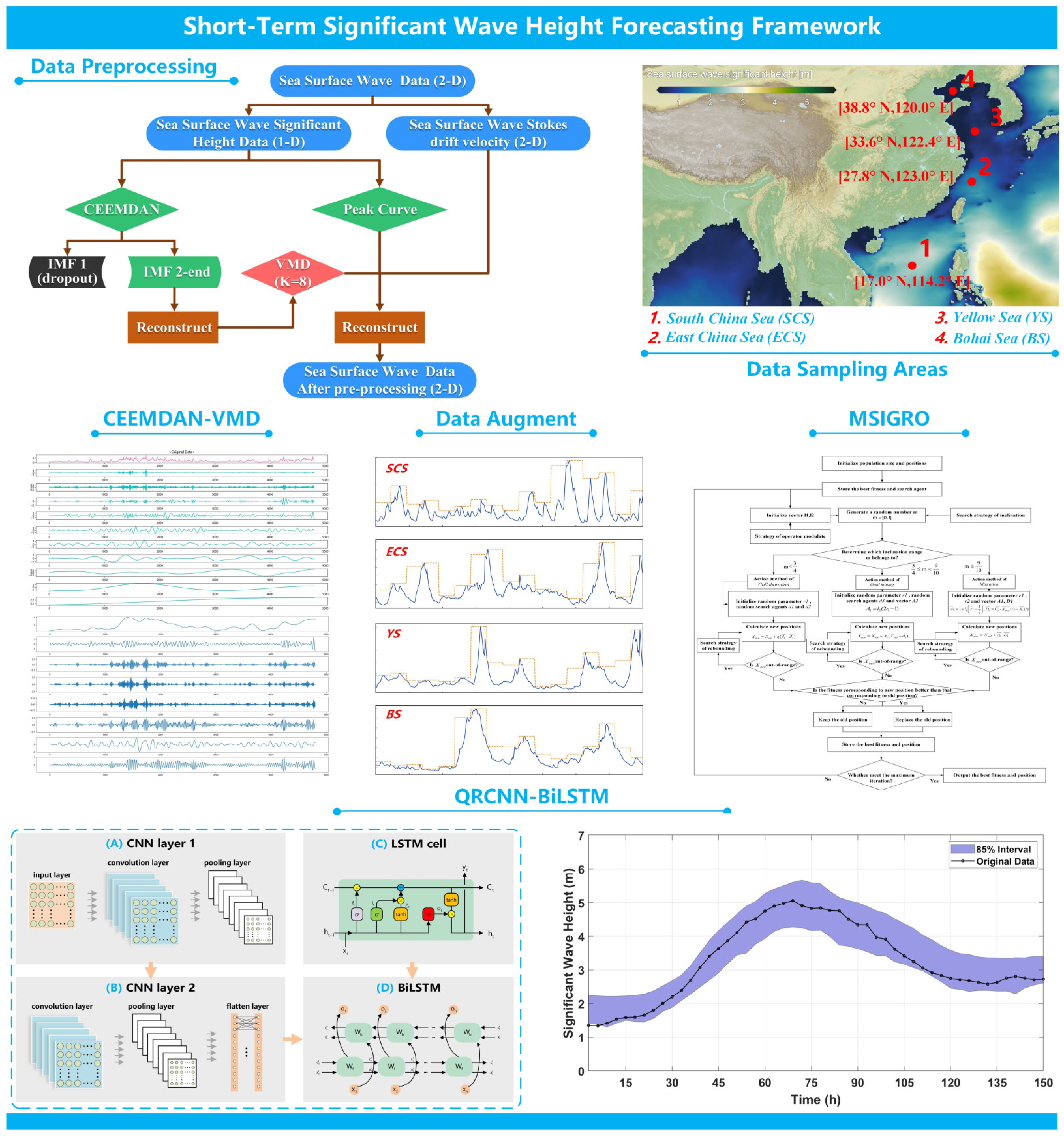
To this end, we propose a significant wave height prediction system based on data preprocessing, combined neural networks, and multi-strategy improved optimization algorithms. The contribution of this paper can be summarized as follows:

(1)

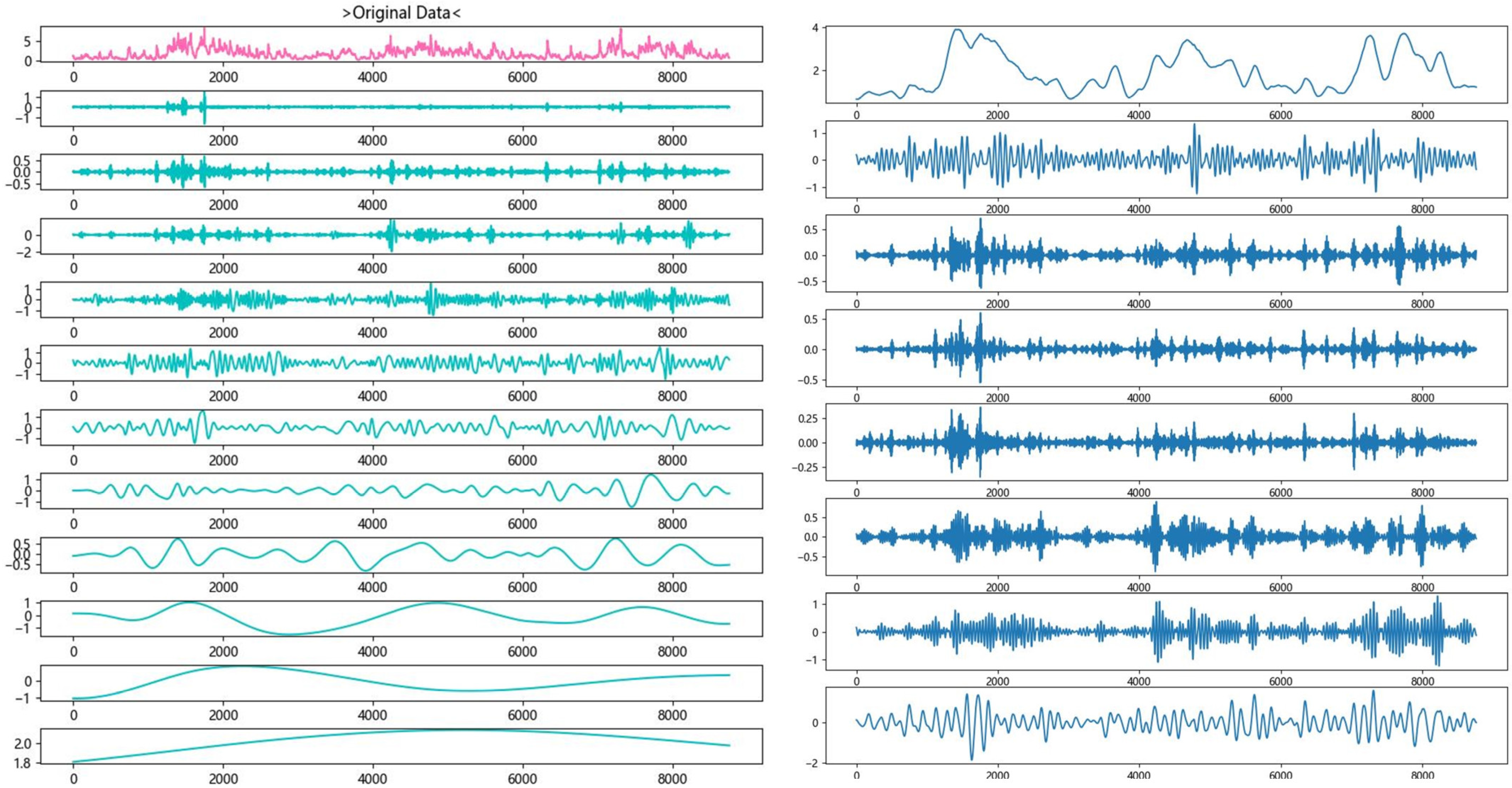
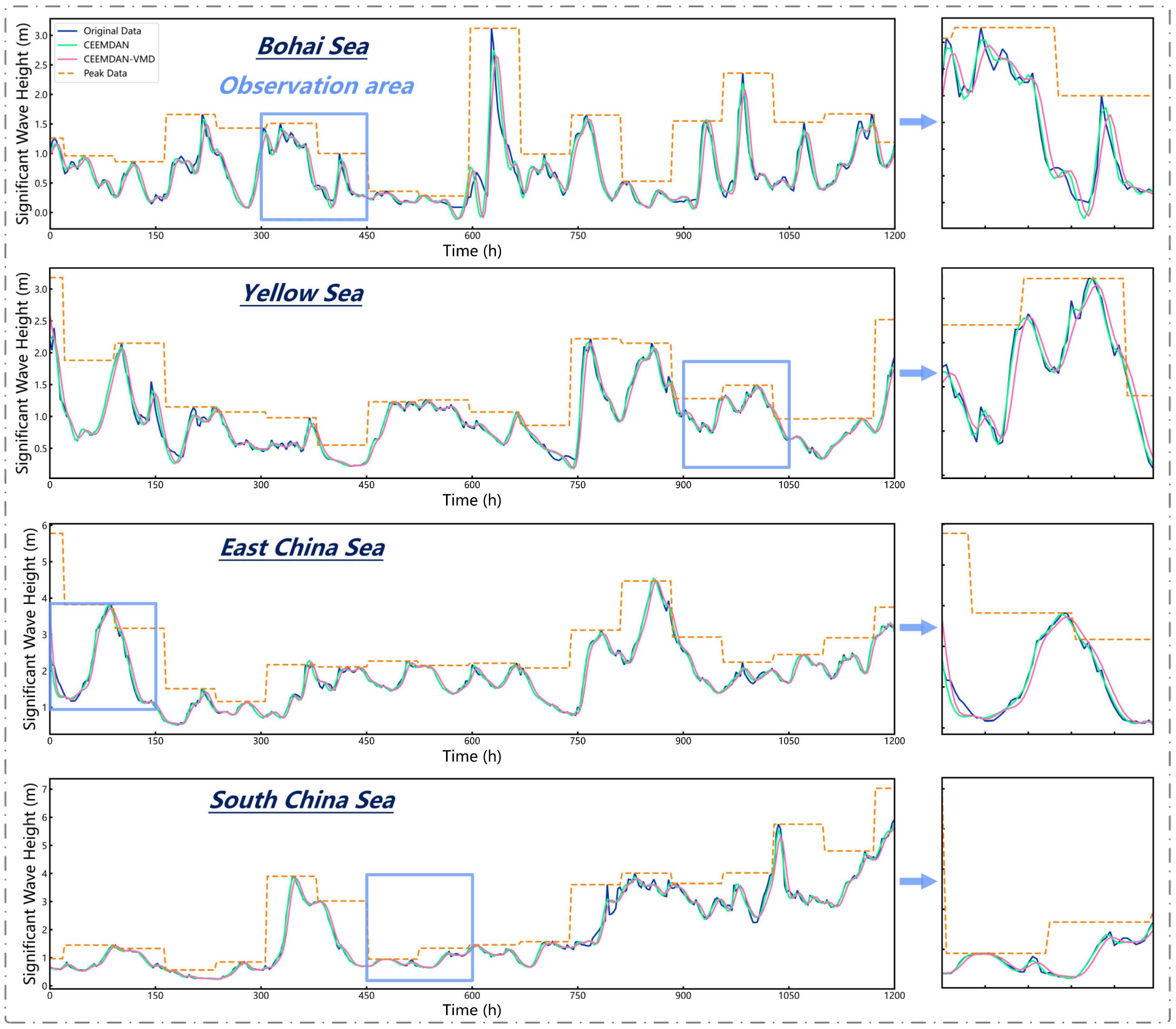
Two techniques of data processing are adopted: data denoising through a hybrid modal decomposition technique of CEEMDAN-VMD and data augmentation by integrating the extracted peak information into the denoised data. These enable the deep learning framework to focus on the trend in wave variations.

(2)

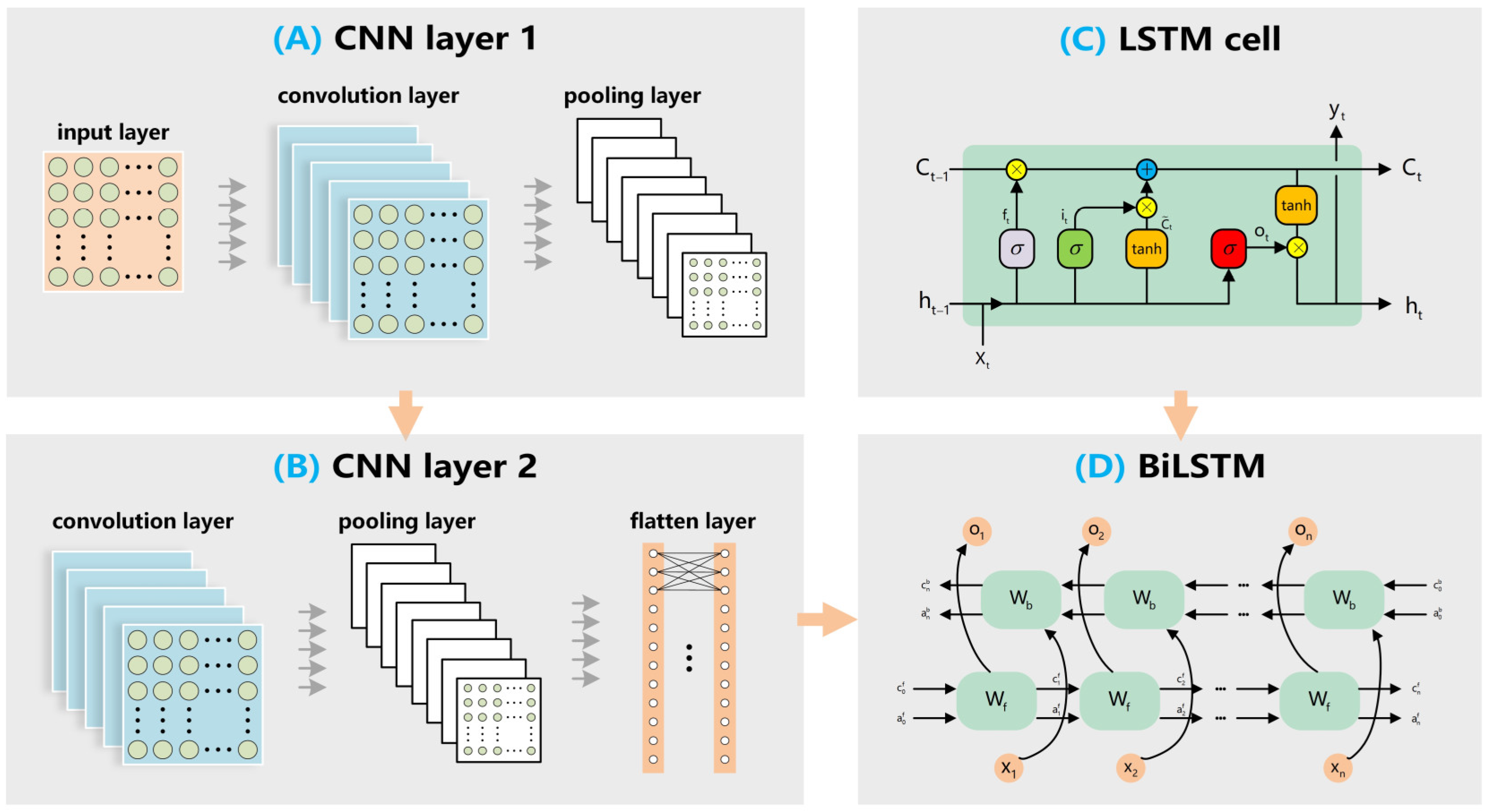
A combination neural network model is developed, consisting of two layers of CNN and one layer of BiLSTM. CNN can identify short-term correlations among various temporal features, and BiLSTM comprises two opposing LSTM layers, which can capture long-term dependencies.

(3)

The quantile regression (QR) is used to achieve interval prediction and introduces three evaluation metrics: PICP, Mean Prediction Interval Width (MPIW), and Average Interval Score (AIS). Compared to others, the proposed method provides a better quality of interval prediction.

(4)

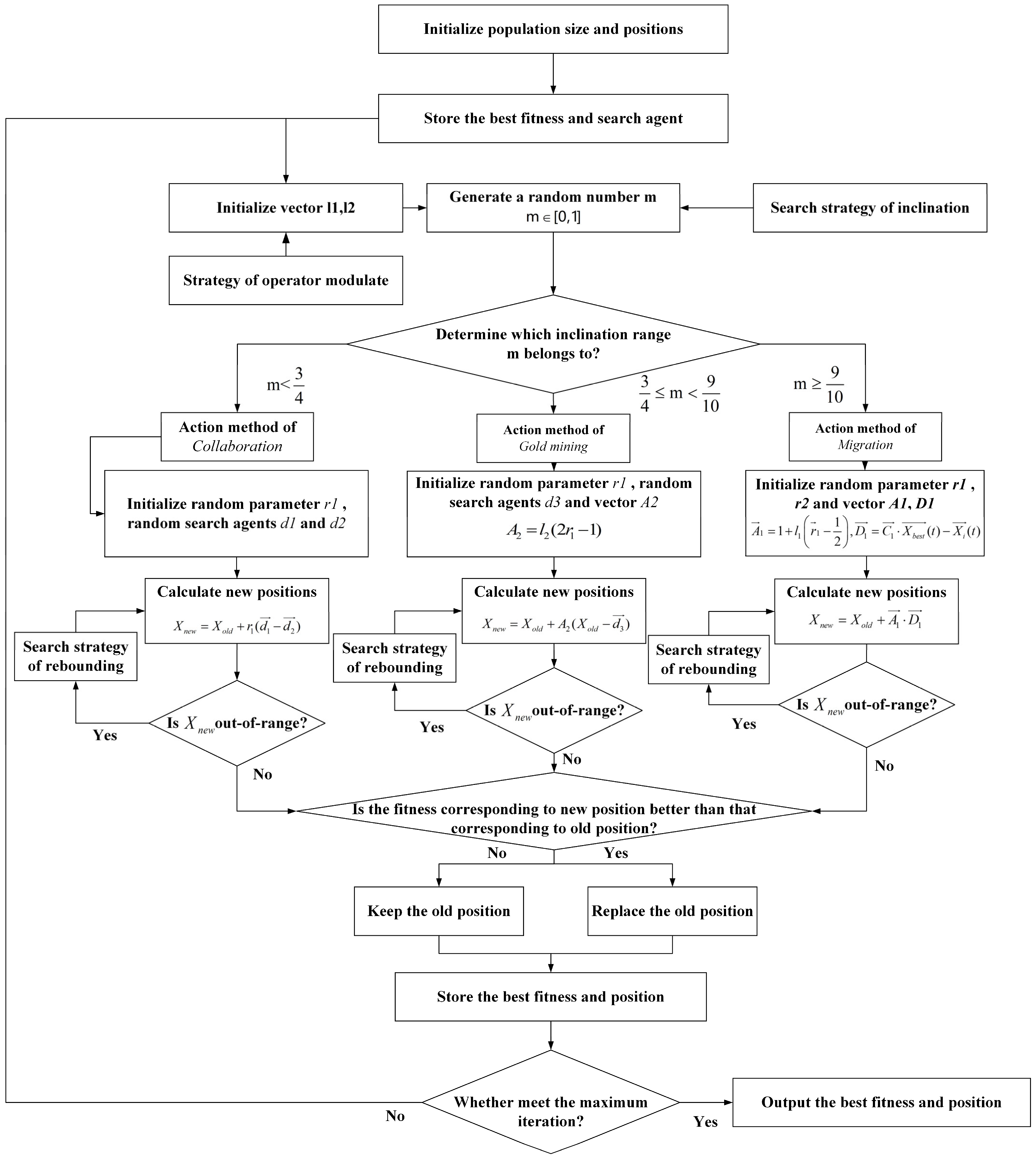
Multi-strategy improved gold rush optimizer (MSIGRO) is utilized to optimize the hyperparameters of the network layers. In high-dimensional optimization space, the original GRO’s ability of optimization is obviously insufficient. Therefore, three improvement strategies are proposed to enhance the algorithm’s optimization ability.

The subsequent chapters of the paper are arranged as follows: Section 2 primarily illustrates the principles of hybrid mode decomposition and the probabilistic deep learning framework. Section 3 will provide the principles of data selection, system parameter design, and system evaluation indexes. Section 4 describes the construction methodology of the significant wave height prediction framework and exhibits the prediction outcomes across four datasets. Section 5 evaluates the proposed framework and other models via four groups of experiments. Finally, Section 6 gives the conclusion.

2. Methodologies

This chapter will first describe the innovative improvement strategies utilized by MSIGRO. Next, we will provide a thorough explanation of the deep learning network model. Finally, the fundamental principles of hybrid mode decomposition will be explained quickly.

2.1. Overall Framework

This study proposes a short-term Hs prediction framework, which can achieve high-quality interval predictions. The framework includes two components: the data processing module and a probabilistic deep learning model. In the data processing module, CEEMDAN-VMD is employed for data denoising, and peak information of the Hs data are extracted for data augmentation. In the probabilistic deep learning module, layers of CNN and BiLSTM will effectively learn features of data, delivering multi-step interval prediction results (12-h periods, 4 steps in total). Furthermore, three innovative strategies are proposed to enhance the GRO for more efficient optimization of hyperparameters in deep learning networks. A flowchart of the proposed method is given in Figure 1. In the next four sections, the data processing and principles of deep learning will be described in detail.

2.2. MSIGRO

To reduce training errors, MSIGRO is applied to figure out the optimal configuration of network parameters, and the algorithmic flow is given in Figure 2. Inspired by the gold rush, the GRO was proposed by Kamran Zolf in [34], which simulates the behaviors of gold prospectors in their fossicking for gold. The population is regarded as a gold mine for explorers in GRO, who engage in types of movements: migration, mining, and cooperation.

To increase the optimization efficiency of the original GRO algorithm, we propose the following improving strategies.

2.2.1. Search Strategy of Rebounding

During the optimization, it is common for the population to surpass the search range, and the conventional approach is to confine them to the boundaries. Nevertheless, in high-dimensional optimization space, the population may converge on the boundaries of various dimensions, resulting in entrapment within the local optimum. Therefore, the search strategy of rebounding is designed as illustrated in Equation (1).

$$\begin{array}{l}\overrightarrow{p}=\overrightarrow{Xne{w}_{i,t}(\dim )}-\overrightarrow{X_{\mathrm{i},t,boundary}(\dim )}\\ \mathrm{if} |\overrightarrow{p}|<{\displaystyle \frac{1}{2}}|\overrightarrow{X_{i,t}(\dim )}|, \mathrm{then} \overrightarrow{X_{i,t}(\dim )}=\overrightarrow{X_{i,t,boundary}(\dim )}-\overrightarrow{p}\end{array}$$

(1)

where $\overrightarrow{Xne{w}_{i,t}(\dim )}$, $\overrightarrow{X_{i,t}(\dim )}$, and $\overrightarrow{X_{\mathrm{i},t,boundary}(\dim )}$, respectively, denote the new position, vector of movement path, and boundary position of the i-th individual in the dim-th dimension in the t-th iteration, and $boundary$ represent $\min$ or $\max$. In this case, the out-of-bounds degree will be evaluated, returning the eligible population to optimization space.

2.2.2. Strategy of Operator Modulation

GRO contains two converging operators $l_1$ and $l_2$, where $l_1$ specifies the action of prospector migration and $l_2$ specifies the action of prospector mining, which are crucial for search efficiency. However, in GRO, there is a bijective relationship between $l_1$, $l_2$, and the iteration $t$. Under this condition, there are low complexities of $l_1$ and $l_2$ and reduced search efficiency. Therefore, the strategy of operator modulation is proposed to assist in optimization, as shown in Equation (2).

$$\begin{array}{l}{l}_{e=1}={\left({\displaystyle \frac{{\max }_{iter}-iter}{{\max }_{iter}-1}}\right)}^e\left(2-{\displaystyle \frac{1}{{\max }_{iter}}}\right)\cdot \sin \left({\displaystyle \frac{iter}{{\max }_{iter}^2}}\right)+{\displaystyle \frac{1}{{\max }_{iter}}}\\ l_{e=2}={\left({\displaystyle \frac{{\max }_{iter}-iter}{{\max }_{iter}-1}}\right)}^e\left(2-{\displaystyle \frac{1}{{\max }_{iter}}}\right)\cdot \cos \left({\displaystyle \frac{iter}{{\max }_{iter}^2}}\right)+{\displaystyle \frac{1}{{\max }_{iter}}}\end{array}$$

(2)

The frequency of the operator $l_e$ will be increased through modulation and still remain converging, improving its flexibility of optimization.

2.2.3. Search Strategy of Inclination

In the original GRO, the behaviors of the population in each iteration are entirely random. Nevertheless, we discover that modifications in the search inclination of the population will affect the optimization efficiency. For instance, an increase in the probability of cooperative actions can decrease the optimization iteration. Based on this regular pattern, we propose the search strategy of inclination, which enables explorers to engage in more effective actions, thus enhancing optimization speed. The grid search method is utilized to customize the parameters of probabilities mentioned above in this research.

2.3. Hybrid Modal Decomposition

A signal decomposition algorithm can decompose complex signals into subcomponents of varying frequencies, facilitating a clear comprehension of time-frequency attributes and hidden features [35]. VMD mitigates problems of modal aliasing and boundary effect in EMD; however, it is susceptible to high-frequency noise, resulting in low accuracy of decomposition.

This study employs a hybrid mode decomposition method that applies VMD to the signal reconstructed post-CEEMDAN decomposition for accurate denoising. By incorporating IMF components with auxiliary noise and executing comprehensive averaging calculations after each decomposition order, CEEMDAN mitigates the transmission of white noise from high to low frequencies. In this case, VMD’s susceptibility to high-frequency noise is effectively relieved.

2.4. Combination Neural Network

The proposed deep learning model comprises two essential neural network components: CNN and BiLSTM. Effectively integrating these layers can enhance prediction performance, as shown in Figure 3.

2.4.1. Convolutional Neural Network

The convolutional neural network is widely used in deep learning tasks. As a specific variant of feedforward neural networks, it extracts local spatial features continuously from images via the movement of convolutional kernels by emulating human visual perception [36]. The essential elements of a convolutional neural network comprise convolutional layers and pooling layers. The input dimensions ($O$) of the convolutional layer are determined in Equation (3).

$$O=(I-K+2P)/S+1$$

(3)

where I and K are the input size of the convolutional layer and the size of the convolutional kernel, respectively. P and S represent the padding size and the convolutional kernel sliding step size, respectively.

Following feature extraction through the convolutional layer, a designated quantity of feature maps is produced and subsequently fed into the pooling layer. The pooling layer executes down-sampling on the feature maps to attain dimensionality reduction, consequently decreasing the number of parameters and computational burden in subsequent network layers, which accelerates the model’s training. A max pooling layer is utilized for data processing, and the output dimension N of the maximum pooling layer can be calculated by Equation (4).

$$N=(I+2P-F)/S+1$$

(4)

where I and P are the pooling layer output size and fill size, respectively, and F and S are the pooling window size and step size, respectively.

Next, the output data will enter the fully connected layer after being activated. We use the LeakyReLu function as the activation function with the expression in Equation (5).

$$LeakyRelu=\max (0,x)+leak\times \min (0,x)$$

(5)

where leak is a very small constant to retain some information about the negative axis.

2.4.2. BiLSTM

The BiLSTM comprises a forward and a backward LSTM, which is a type of recurrent neural network (RNN) proposed to solve the problems in conventional RNN, for instance, long-term dependencies and gradient explosion [37]. Components of LSTM include input gates, forget gates, and output gates.

Component 1: Input Gate

The input gate reads the contents of $h_{t-1}$ and $x_t$; this determines whether the information will be retained in the cell state $c_t$. The formula is shown in Equations (6)–(8), where $\sigma$ represents the sigmoid function; $h_{t-1}$ and $x_t$ are the inputs; $W$ and $b$ are the learnable weights; and $\widetilde{{\mathrm{c}}_t}$ employs the $\tanh$ activation function for the candidate states.

$$\begin{array}{c}{\mathrm{i}}_t=\sigma (W_{ix}{x}_t+b_{ix}+W_{ih}{h}_{t-1}+b_{ih})\\ \widetilde{{\mathrm{c}}_t}=\tanh (W_{cx}{x}_t+b_{cx}+W_{ch}{h}_{t-1}+b_{ch})\end{array}$$

(6)

Component 2: Oblivion Gate

The forgetting gate determines the discarding and retention of information in the previous state with the following formula:

$$f_t=\sigma (W_{fx}{x}_t+b_{fx}+W_{fh}{h}_{t-1}+b_{fh})$$

(7)

Component 3: Output Gate

The output gate is used to determine the next hidden state and which information in the memory cell controls the current output. The equation for an output gate is as follows:

$$\begin{array}{l}{o}_t=\sigma (W_{ox}{x}_t+b_{ox}+W_{oh}{h}_{t-1}+b_{oh})\\ h_t=o_t*\tanh (c_t)\end{array}$$

(8)

2.5. Quantile Regression

Point prediction models assess the efficacy of predictions by comparing predicted values with actual ones; however, they may exhibit low accuracy in extreme conditions. This paper attempts to construct a probabilistic deep learning model utilizing the quantile regression (QR), which was proposed by Koenker et al. in 1978 [38]. By examining the conditional quantile relationship between independent and dependent variables, a regression model will be established. Expression of QR is formulated in Equations (9)–(13):

Supposing that there are $n$ explanatory variables $U=\left\{U_1,U_2,\dots ,U_n\right\}$ acting on random variables $S$, the distribution function of $S$ can be expressed as follows:

$$F(s)=P(S\le s)$$

(9)

For any quantile $\tau \in \left[0,1\right]$, there is:

$$F^{-1}(\tau )=\inf \left\{s:F\left(s\right)\ge \tau \right\}$$

(10)

where $F^{-1}$ is the $\tau -\mathrm{th}$ quantile of $S$, and $\inf$ is the lower bound of the set $s$.

In the QR model, the $\tau$-th conditional quantile of the response variable $S$ under the explanatory variable $U$ is as follows:

$$\begin{array}{l}{\mathrm{Q}}_S\left(\tau |U\right)={\beta }_0\left(\tau \right)+{\displaystyle \sum _{i=1}^c{\beta }_i\left(\tau \right)}\\ U_i=U’\beta \left(\tau \right)\end{array}$$

(11)

where the parameters associated with $\beta \left(\tau \right)$ can be solved by the loss function as follows:

$$\underset{\beta }{\min }{\displaystyle \sum _{i=1}^N{\rho }_{\tau }}\left(S_i-U_i’\beta \right)=\underset{\beta }{\min }{\displaystyle \sum _{i|S_i\ge U_i’\beta }\tau |S_i-U_i’\beta |}+{\displaystyle \sum _{i|S_i\ge U_i’\beta }(1-\tau )|S_i-U_i’\beta |}$$

(12)

where ${\rho }_{\tau }$ is the test function and it is expressed as follows:

$$\begin{array}{l}{\rho }_{\tau }\left(\mu \right)=\mu (\tau -I(\mu ))\\ I(\mu )=\left\{\begin{array}{c}1,\mu <0\\ 0,\mu \ge 0\end{array}\right.\end{array}$$

(13)

3. Dataset Selection and Parameter Design

3.1. Dataset Selection

The Bohai, Yellow, East China, and South China Seas are the most crucial ocean routes of China, carrying value of energy and strategy. Precisely forecasting the Hs in these regions is of great reference value for wave energy development and marine operations. The locations of buoy stations for data collection in this study are as follows: Bohai Sea [38.8° N, 120.0° E], Yellow Sea [33.6° N, 122.4° E], East China Sea [27.8° N, 123.0° E], and South China Sea [17.0° N, 114.2° E]. These sites are geographically representative, with varied latitudes and depths, and subject to a broad range of climates from tropical to temperate climates; moreover, these sites cover key shipping lanes, fishery zones, energy development areas, and eco-sensitive regions, providing data from varied regions from coastal areas to deep waters, and data under both normal and extreme conditions.

The dataset utilized in this study is sourced from the Copernicus Marine Service database (Copernicus). Based on comprehensive analysis of coastal wave dynamics in our study regions (the lifespan of a typhoon typically ranges from 3 to 8 days), 96 steps (covering a 12-day window) are selected to capture the wave patterns and maintain computational efficiency. The 12-, 24-, and 36-h forecasts are selected to provide an optimal balance between prediction accuracy and extended-range forecasting capability. Shorter forecasting steps (3 h and 6 h) were excluded from our study due to their limited operational utility, while forecasts beyond 48 h exhibit deterioration in prediction quality. The wind is a main cause for the generation and motion of waves in seas; though there are strong variations in the wind speed and direction under extreme weather conditions, the wave height (Hs) and velocity well reflect the complex impacts of wind on waves, and the wave velocity, to some extent, indicates the wind speed and direction. Data on flow velocities (horizontal and vertical) and Hs are gathered over three years from the specified four marine regions. This data collection method reduces the computing overhead, making it possible for large-scale deployment of buoy stations and wave forecasting globally. Through the chronological split method, the first 80% of the dataset (from January 2021 to May 2023) is considered the training set, while the remaining data (from June 2023 to December 2023) serve as the test set [23,28]. Feature engineering is performed independently in the training set before the same engineering rules are applied to the test set to preclude data leakage.

3.2. Parameter Design

This paper proposes a prediction model that employs the CEEMDAN-VMD hybrid modal decomposition technique for data preprocessing and extracts wave peak information for data augmentation. A CNN-BiLSTM network, enhanced by a multi-strategy improved GRO, is employed for prediction.

Table 1. Super-parameters of the Hs forecasting system.

Model	Parameters	Value
CEEMDAN	Trials	100
	$\epsilon$ (Signal–Noise Ratio)	0.005
VMD	$\alpha$	1300
	$\tau$	0
	K	8
	DC	1
	Init	1
	Tol	1 × 10−7
Deep Learning	Time Step	96
	Time Step Feature	4
	Batch Size	128
	Training Epoch	100
	Output Size	4

shows hyperparameters for the hybrid modal decomposition and the deep learning model. The ε value in CEEMDAN is set to 0.005 to achieve a balance between denoising and preserving essential information. For VMD, the decomposition number K is set to 8 to avoid inadequate or excessive decomposition.

3.3. Evaluation Indexes

The probabilistic deep learning trains the framework by establishing various quantiles to achieve interval prediction at various confidence levels. To assess the effectiveness and accuracy of the prediction results at various levels of PINC, indexes (PICP, MPIW, AIS, RMSE, MAE) are involved. The equation is given in Equations (14)–(19):

$$PICP={\displaystyle \frac{1}{n}}{\displaystyle \sum _{i=1}^n(T_i\in [L(P_i),U(P_i)])}$$

(14)

$$MPIW={\displaystyle \frac{1}{n}}{\displaystyle \sum _{i=1}^n(U(P_i)-L(P_i))}$$

(15)

$$AIS={\displaystyle \frac{1}{n}}{\displaystyle \sum _{i=1}^{n}S(P_i)}$$

(16)

$$S(P_i)=\left\{\begin{array}{l}-0.02\times alpha\times (U(P_i)-L(P_i))-4\times (L(P_i)-T_i) \mathrm{if} T_i<L(P_i)\\ -0.02\times alpha\times (U(P_i)-L(P_i)) \mathrm{if} L(P_i)\le T_i\le U(P_i)\\ -0.02\times alpha\times (U(P_i)-L(P_i))-4\times (T_i-U(P_i)) \mathrm{if} T_i>U(P_i)\end{array}\right.$$

(17)

$$RMSE=\sqrt{{\displaystyle \frac{1}{n}}{\sum }_{i=1}^n{(y_i-\widehat{y_i})}^2}$$

(18)

$$MAE={\displaystyle \frac{1}{m}}{\sum }_{i=1}^m\left|\left(y_i-\widehat{y_i}\right)\right|$$

(19)

where $L(P_i)$ and $U(P_i)$ represent the prediction results at the lower and upper bounds of the interval at the time $i$, respectively; $P_i$ is the set quantile; $T_i$ represents the true value of the effective wave height at the time i; and alpha is a customized parameter with a value of 1000. PICP is the interval coverage, which is defined as the proportion of true values between the upper and lower bounds of the interval. When the value of PICP is greater than the set confidence level, the prediction result is considered valid. $MPIW$ is the average interval width, and a smaller value of MPIW indicates a narrower interval width and a more accurate prediction result. AIS means average interval score, which measures the quality of interval prediction by considering coverage rate and interval width comprehensively. A higher average interval score indicates superior prediction quality of the model (e.g., at equal coverage, intervals with AIS of −20 outperform AIS of −30). RMSE is the root mean square error, and MAE means mean absolute error. The mean value of the forecasts of the quantiles at every 0.05 interval from the lower to the upper bounds is considered the point forecast result to calculate RMSE and MAE for assessment of the model’s performance. The performance of the deep learning framework can be evaluated objectively and comprehensively through these evaluation indexes. Per the classification of marine safety levels, the predicted PINC values are divided into three levels—0.85, 0.90, and 0.95. The 0.85 PINC corresponds to the safe operating cordon for small boats, applicable to regular navigation planning; the 0.90 PINC corresponds to the safe operating cordon for large commercial ships, applicable to cargo handling decision-making and assessment, and hence forecasts at this level demonstrate the model’s reliability under high-risk conditions; the 0.95 PINC corresponds to the threshold for port closure, applicable to emergency management planning, and forecasts at this level demonstrate the early warning capacity of a region against extreme weather events.

3.4. Operating Environment

The basic operating environment for the Hs prediction model proposed in this study is Intel Core i7-12700F and RTX 4070. The data processing module employs PyCharm 2024, and the deep learning framework is developed by MATLAB 2023b.

4. Deep Learning Framework Design and Prediction Results

This chapter will make detailed introductions of the subsystems in the proposed Hs prediction system and assess its robustness and generalization on the four datasets.

4.1. Data Preprocessing System Design

The generation of waves is notably complex, primarily influenced by sea wind, which exhibits instantaneity, resulting in the convergence of numerous wave patterns on the ocean’s surface. These waves originate from different locations, which possess diverse velocities and propagation orientations. Consequently, it is inadequate to capture information from the one-dimensional Hs data. To this end, CEEMDAN-VMD is applied for data denoising, and peak information is integrated into the denoised dataset as a data augmentation. Specifically, the maximum of the Hs every 72 h serves as the peak information of the period.

The data processed through the above methods are visualized as follows: Figure 4 shows the modal components of CEEMDAN-VMD, and Figure 5 displays the data after processing by different methods.

Table 2. Characteristics of different data processing methods.

	Dimensions	Max	Min	Mean	Var	Std
Bohai Sea	Original Data	4.56	0.0300	0.7607	0.3101	0.5568
	Peak	4.56	0.1100	0.9986	0.4362	0.6604
	Wavelet	4.46	0.0102	0.7608	0.3082	0.5551
	EMD	4.61	0.0010	0.7623	0.3087	0.5556
	CEEMDAN	4.65	0.0001	0.7618	0.3082	0.5551
	CEEMDAN-VMD	4.62	0.0015	0.7618	0.2988	0.5466
Yellow Sea	Original Data	5.28	0.1600	1.0948	0.3759	0.6131
	Peak	5.28	0.1900	1.3119	0.5654	0.7519
	Wavelet	5.28	0.1336	1.0948	0.3746	0.6121
	EMD	5.00	0.1452	1.0953	0.3776	0.6145
	CEEMDAN	5.02	0.1597	1.0951	0.3732	0.6109
	CEEMDAN-VMD	4.62	0.1634	1.0952	0.3681	0.6067
East China Sea	Original Data	7.31	0.5300	1.7293	0.6514	0.8071
	Peak	7.31	0.5900	1.9821	1.0597	1.0294
	Wavelet	7.29	0.5200	1.7292	0.6495	0.8059
	EMD	7.17	0.2907	1.7306	0.6542	0.8088
	CEEMDAN	7.17	0.5049	1.7303	0.6492	0.8057
	CEEMDAN-VMD	6.93	0.5231	1.7303	0.6409	0.8006
South China Sea	Original Data	8.35	0.1900	1.8716	1.4862	1.2191
	Peak	8.35	0.2700	2.0822	1.8721	1.3683
	Wavelet	8.34	0.1791	1.8715	1.4853	1.2187
	EMD	7.82	0.1881	1.8712	1.4850	1.2186
	CEEMDAN	7.82	0.1892	1.8710	1.4834	1.2179
	CEEMDAN-VMD	7.80	0.1898	1.8710	1.4721	1.2133

illustrates the features of four datasets subsequent to various processing techniques. The wavelet transform was applied through adaptive thresholding of decomposed coefficients (Symlet-4, four levels), automatically estimating noise characteristics from high-frequency components while preserving physical signal structures. The variance of the data applying the hybrid modal decomposition is the least, considerably reducing the non-stationarity of the Hs.

4.2. Deep Learning Predictive Model Design

4.2.1. Design Principles

Table 3. Structures and parameters in deep learning systems.

	Parameters	Value
Conv1d 1	Input Size	96
	NumFilters	13 (Based on MSIGRO)
	Kernel Size	3
MaxPool 1	Kernel Size	3
	Stride	1
	Padding	Same
Conv1d 2	Input Size	13 (Based on MSIGRO)
	NumFilters	11 (Based on MSIGRO)
	Kernel Size	3
MaxPool 2	Kernel Size	3
	Stride	1
	Padding	Same
BiLSTM	Hidden Units	12 (Based on MSIGRO)
Dropout	Drop Rate	0.1
Training Options	Learning Rate	6.6 × 10−3 (Based on MSIGRO)

presents the structure of the CNN-BiLSTM deep learning model, the design of which is motivated by the following factors:

(1)

In Hs prediction, while single-step forecasts may attain considerable accuracy, they fall short of foresight. Instead, an excessively large time step will diminish the capacity of the deep learning model to capture local features. Thus, we designate 96 steps (3 × 96 h) for each training data batch and 12 h for prediction. Based on the above processing, CNN is adopted for feature extraction from the data.

(2)

Given that CNN is incapable of learning long-term seasonal nature, the incorporation of BiLSTM rectifies this shortcoming. The LSTM of BiLSTM includes distinct memory cells and gating mechanisms, enabling it to effectively manage long-term dependencies in time series data. Consequently, the CNN-BiLSTM combined model can perform better than single ones in learning data patterns.

4.2.2. Performance Evaluation

This study utilizes four sets of Hs data, with the visualized prediction outcomes displayed in Figure 6 and

Table 4. Short-term Hs forecasting results.

	PINC = 0.85					PINC = 0.90					PINC = 0.95
	PICP	MPIW	AIS	RMSE	MAE	PICP	MPIW	AIS	RMSE	MAE	PICP	MPIW	AIS	RMSE	MAE
Bohai Sea	0.88	0.7138	−14.3281	0.1872	0.1484	0.94	0.8756	−17.5424	0.1801	0.1419	1.00	1.3518	−27.0359	0.2096	0.1675
Yellow Sea	0.94	0.7942	−15.9399	0.2497	0.1536	0.96	1.0424	−20.8515	0.3243	0.2006	1.00	1.3058	−26.1155	0.2956	0.1808
East China Sea	0.88	0.6959	−14.0351	0.2865	0.1847	0.96	0.8709	−17.4316	0.2778	0.1694	1.00	1.3531	−27.0615	0.2622	0.1643
South China Sea	0.96	1.0975	−21.9570	0.2187	0.1836	1.00	1.3864	−27.7283	0.3060	0.2571	1.00	1.4433	−28.8652	0.2275	0.1955

. The proposed prediction system demonstrates excellent coverage rate and optimal interval prediction results across all four datasets.

5. Four Groups of Experiments

This chapter analyzes and contrasts the proposed prediction model through four groups of experiments, validating the criticality of data processing, the benefits of customizing deep learning networks compared to baseline models, the enhancement effects of the proposed improved strategies of the algorithm, and various forecasting time periods.

5.1. Experiment 1

We compared the data processed through denoising and augmentation with that processed by other methods, while maintaining the CNN-BiLSTM framework unchanged.

Table 5. Forecasting results of different data processing methods in Experiment 1.

		PINC = 0.85					PINC = 0.90					PINC = 0.95
		PICP	MPIW	AIS	RMSE	MAE	PICP	MPIW	AIS	RMSE	MAE	PICP	MPIW	AIS	RMSE	MAE
Bohai Sea	Original Data	0.72	0.6662	−13.5017	0.2141	0.1657	0.84	0.8452	−17.0107	0.2057	0.1562	0.96	1.3071	−26.1479	0.1972	0.1476
	Without MD	0.82	0.5454	−10.9886	0.1686	0.1319	0.90	0.8173	−16.3863	0.1752	0.1401	1.00	1.4578	−29.1565	0.1401	0.1141
	Without Peak	0.88	0.9494	−19.0711	0.1740	0.1425	0.94	1.2615	−25.2424	0.2046	0.1633	0.98	1.4010	−28.0190	0.2002	0.1622
	Without VMD	0.80	0.6510	−13.0777	0.1624	0.1287	0.90	0.8584	−17.1948	0.1398	0.1095	0.96	0.8901	−17.8226	0.1395	0.1119
	Proposed Method	0.88	0.7138	−14.3281	0.1872	0.1484	0.94	0.8756	−17.5424	0.1801	0.1419	1.00	1.3518	−27.0359	0.2096	0.1675
Yellow Sea	Original Data	0.82	0.8710	−17.5692	0.2470	0.1819	0.90	1.5129	−30.2672	0.2487	0.1774	0.96	1.2963	−25.9880	0.2865	0.2128
	Without MD	0.84	0.9331	−18.6263	0.1670	0.1296	0.92	1.1350	−22.7191	0.1535	0.1111	0.98	1.6005	−32.0133	0.1893	0.1469
	Without Peak	0.84	0.9641	−19.4268	0.3017	0.2086	0.94	1.1881	−23.8273	0.3128	0.2101	1.00	1.4919	−29.8380	0.3919	0.2573
	Without VMD	0.84	1.0271	−20.6449	0.2001	0.1515	0.96	1.1934	−23.8679	0.1257	0.1032	1.00	1.3960	−27.9194	0.1527	0.1164
	Proposed Method	0.94	0.7942	−15.9399	0.2497	0.1536	0.96	1.0424	−20.8515	0.3243	0.2006	1.00	1.3058	−26.1155	0.2956	0.1808
East China Sea	Original Data	0.76	0.6234	−12.5750	0.1932	0.1252	0.86	1.0486	−21.2044	0.2061	0.1411	0.98	1.2828	−25.6965	0.2024	0.1393
	Without MD	0.84	0.4668	−9.3950	0.1787	0.1296	0.92	0.9032	−18.0756	0.1812	0.1339	1.00	1.5300	−30.6288	0.1792	0.1236
	Without Peak	0.86	0.7280	−14.7883	0.2901	0.1792	0.88	1.0462	−21.1864	0.3220	0.2062	1.00	1.8846	−27.6916	0.2893	0.1803
	Without VMD	0.82	0.8043	−16.1239	0.1670	0.1324	0.90	1.0003	−20.0299	0.1548	0.1137	1.00	1.7168	−34.3360	0.1643	0.1067
	Proposed Method	0.88	0.6959	−14.0351	0.2865	0.1847	0.96	0.8709	−17.4316	0.2778	0.1694	1.00	1.3531	−27.0615	0.2622	0.1643
South China Sea	Original Data	0.78	0.9017	−18.0801	0.2976	0.2218	0.86	1.1093	−22.264	0.2995	0.2274	1.00	2.7265	−54.5291	0.2173	0.1802
	Without MD	0.94	1.3332	−26.7022	0.2439	0.1971	1.00	2.5237	−50.4748	0.2050	0.1749	1.00	2.5900	−51.7998	0.2542	0.2006
	Without Peak	0.94	1.6640	−33.2844	0.3648	0.2851	1.00	2.2777	−45.5530	0.2842	0.2309	1.00	3.3335	−66.6705	0.2968	0.2394
	Without VMD	0.84	1.6894	−34.0050	0.3801	0.2924	1.00	1.9066	−38.1326	0.2999	0.2291	1.00	2.6397	−52.7942	0.2473	0.1838
	Proposed Method	0.96	1.0975	−21.9570	0.2187	0.1836	1.00	1.3864	−27.7283	0.3060	0.2571	1.00	1.4433	−28.8652	0.2275	0.1955

illustrates the experimental outcomes of various data processing techniques, and

Table 6. Forecasting results of different modal decomposition methods in Experiment 1.

		PINC = 0.85					PINC = 0.90					PINC = 0.95
		PICP	MPIW	AIS	RMSE	MAE	PICP	MPIW	AIS	RMSE	MAE	PICP	MPIW	AIS	RMSE	MAE
Bohai Sea	EMD	0.82	0.4900	−10.0323	0.1596	0.1209	0.90	0.7539	−15.1303	0.1477	0.1138	0.96	1.1776	−23.5557	0.1521	0.1184
	VMD	0.86	0.9264	−18.5772	0.1981	0.1594	0.94	1.3150	−26.3501	0.1967	0.1569	0.98	1.7530	−35.0635	0.1995	0.1606
	CEEMDAN	0.80	0.6510	−13.0777	0.1624	0.1287	0.90	0.8584	−17.1948	0.1398	0.1095	0.96	0.8901	−17.8226	0.1395	0.1119
	Wavelet	0.90	0.7429	−14.8962	0.1208	0.0972	0.92	0.6747	−13.5079	0.1163	0.0863	1.00	1.3972	−27.9446	0.1698	0.1344
	CEEMDAN-VMD	0.88	0.7138	−14.3281	0.1872	0.1484	0.94	0.8756	−17.5424	0.1801	0.1419	1.00	1.3518	−27.0359	0.2096	0.1675
Yellow Sea	EMD	0.80	0.8200	−16.7373	0.2398	0.1949	0.96	1.3050	−26.1089	0.1823	0.1526	1.00	1.5230	−30.4602	0.1580	0.1308
	VMD	0.84	0.8281	−16.6414	0.2883	0.1811	0.92	0.9671	−19.3543	0.2923	0.1942	0.94	1.3766	−27.5640	0.2836	0.1785
	CEEMDAN	0.84	1.0271	−20.6449	0.2001	0.1515	0.96	1.1934	−23.8679	0.1257	0.1032	1.00	1.3960	−27.9194	0.1527	0.1164
	Wavelet	0.92	1.0502	−21.0267	0.2380	0.1767	0.96	1.0987	−21.9898	0.2155	0.1672	1.00	1.3360	−26.7203	0.2102	0.1689
	CEEMDAN-VMD	0.94	0.7942	−15.9399	0.2497	0.1536	0.96	1.0424	−20.8515	0.3243	0.2006	1.00	1.3058	−26.1155	0.2956	0.1808
East China Sea	EMD	0.80	0.4434	−9.1748	0.1682	0.1284	0.88	0.7589	−15.2225	0.1657	0.1153	0.94	1.2211	−24.4418	0.1789	0.1361
	VMD	0.86	0.8116	−16.2728	0.2782	0.1793	0.90	0.93209	−18.6755	0.2545	0.1758	0.94	1.2506	−25.0528	0.2667	0.1725
	CEEMDAN	0.82	0.8043	−16.1239	0.1670	0.1324	0.90	1.0003	−20.0299	0.1548	0.1137	1.00	1.7168	−34.3360	0.1643	0.1067
	Wavelet	0.82	0.8387	−16.8190	0.1769	0.1431	0.96	1.0462	−20.9390	0.1992	0.1520	1.00	1.3936	−27.8715	0.2078	0.1569
	CEEMDAN-VMD	0.88	0.6959	−14.0351	0.2865	0.1847	0.96	0.8709	−17.4316	0.2778	0.1694	1.00	1.3531	−27.0615	0.2622	0.1643
South China Sea	EMD	0.84	1.3849	−27.7314	0.2617	0.1972	0.98	2.2016	−44.0321	0.2463	0.1845	1.00	2.3341	−46.6828	0.2394	0.1999
	VMD	0.92	1.2258	−24.5429	0.2243	0.1787	0.96	1.2535	−25.0839	0.2104	0.1660	1.00	2.2405	−44.8109	0.2492	0.2176
	CEEMDAN	0.84	1.6894	−34.0050	0.3801	0.2924	1.00	1.9066	−38.1326	0.2999	0.2291	1.00	2.6397	−52.7942	0.2473	0.1838
	Wavelet	0.90	1.7757	−35.5279	0.3296	0.2656	0.98	1.2806	−25.6155	0.3657	0.3063	1.00	3.0059	−60.1182	0.4218	0.3589
	CEEMDAN-VMD	0.96	1.0975	−21.9570	0.2187	0.1836	1.00	1.3864	−27.7283	0.3060	0.2571	1.00	1.4433	−28.8652	0.2275	0.1955

shows the results of different modal decomposition methods.

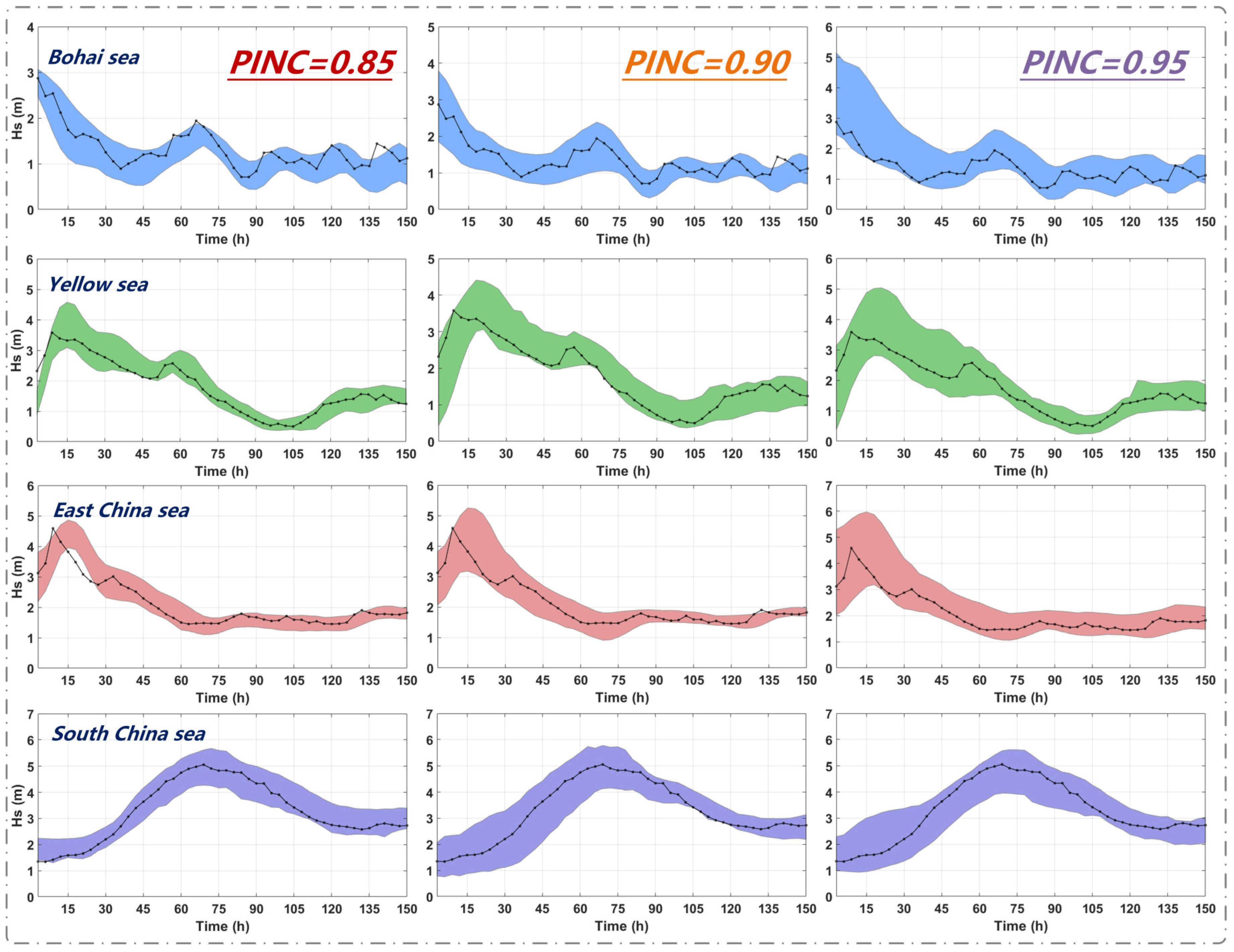
In Table 5, with a PINC of 0.85, the PICP of the proposed method for the Bohai Sea data is 0.88, exhibiting a 16% increase compared to the prediction results of the unprocessed data. However, the RMSE under the three PINCs is higher than the values obtained by other methods in the majority of test cases. In the Yellow Sea data, when PINC is 0.90, the interval coverage remains consistent with CEEMDAN (without VMD); however, the average interval width is reduced, which means more accuracy. The interval score of unprocessed data is notably higher at −15.115, but with a PICP of 0.82, resulting in an invalid prediction. Compared with the forecasts based on the original data (with a PICP of 0.90 and an RMSE of 0.2487), the processing method with CEEMDAN alone shows little effect in increasing the interval forecast performance, but when combined with data augmentation, it reduces the RMSE from 0.1535 to 0.1257. The introduction of VMD reduces the model’s point forecast performance because of deeper denoising but improves the interval forecast performance. In the East China Sea data, when PINC is 0.95, the AIS of the proposed method is −27.0615, exceeding other methods. The South China Sea data exhibit worse stationarity, complicating predictions and leading to generally wider intervals than those of other regions. The PINC 0.95 prediction results indicate that, at the same coverage, the interval width of the proposed method is 1.4433 with the highest AIS. Though the CEEMDAN-VMD method reduces the RMSE by around 15%, it achieves broader coverage at a narrower interval width, and thus, comprehensively, forecasts obtained this way are considered more reliable.

Table 6 illustrates an evaluation of the influence of various modal decomposition methods on predictive performance, with data augmentation techniques remaining constant. At a PINC of 0.85, the proposed CEEMDAN-VMD method demonstrates a notable enhancement in the data from the Yellow Sea and East China Sea. At a PINC of 0.90, across the majority of datasets (Bohai Sea, Yellow Sea, South China Sea), numerous methods exhibit nearly the same interval coverage capabilities; however, CEEMDAN-VMD shows superior prediction quality with the narrowest interval width. The wavelet decomposition method shows stable performance in interval prediction and outperforms the method with VMD alone, and with a smaller RMSE, the CEEMDAN-VMD method demonstrates excellent performance in both point and interval forecasting. When the PINC is 0.95, other approaches fail to attain comprehensive coverage across all datasets, demonstrating that the proposed method exhibits the most robust generalization capability. At deep water regions (South China Sea), the wavelet decomposition method achieves a higher RMSE than other methods, but its RMSE and MAE on the other three datasets (Bohai Sea, Yellow Sea, and East China Sea) are generally lower than the other methods, indicating that this method is more suitable for forecasting in shallower water regions.

5.2. Experiment 2

This experiment primarily validates the necessity of customized prediction models for ocean wave height data. We compared the prediction results of the CNN, LSTM, GRU (

Table 7. Parameters of baseline models in Experiment 2.

Model	Layer	Parameters	Value
CNN	Conv1d	Input Size	96
		Kernel Size	3
		Padding	1
	Maxpooling1d	Kernel Size	3
		Stride	1
LSTM	LSTM	Layer Number	1
		Hidden Units	64
GRU	GRU	Layer Number	1
		Hidden Units	64

), and CNN-BiLSTM while maintaining complete consistency in the data processing system and optimization algorithms. The experimental evaluation indexes show that the deep learning framework in this paper outperformed the baseline model in prediction accuracy. The experimental results are given in

Table 8. Forecasting results of different models in Experiment 2.

		PINC = 0.85					PINC = 0.90					PINC = 0.95
		PICP	MPIW	AIS	RMSE	MAE	PICP	MPIW	AIS	RMSE	MAE	PICP	MPIW	AIS	RMSE	MAE
Bohai Sea	CNN	0.70	1.0933	−22.1299	0.3782	0.3047	0.88	1.5622	−31.3010	0.3233	0.2608	0.94	2.1371	−42.8504	0.3255	0.2559
	LSTM	0.82	0.8536	−17.1540	0.2259	0.1776	0.90	1.0491	−21.0237	0.2399	0.1901	0.98	1.2966	−25.9344	0.2297	0.1821
	GRU	0.80	0.6186	−12.5110	0.2304	0.1850	0.88	0.8811	−17.6949	0.2298	0.1844	1.00	1.3774	−27.5486	0.2344	0.1926
	CNN-BiLSTM	0.88	0.7138	−14.3281	0.1872	0.1484	0.94	0.8756	−17.5424	0.1801	0.1419	1.00	1.3518	−27.0359	0.2096	0.1675
Yellow Sea	CNN	0.80	0.8993	−18.2754	0.4892	0.3741	0.94	1.1358	−22.7269	0.4323	0.3310	0.98	1.485	−29.7201	0.4281	0.3284
	LSTM	0.82	0.9782	−19.5979	0.3052	0.1851	0.96	1.0939	−21.8857	0.3037	0.1875	1.00	1.5815	−31.6294	0.2969	0.1821
	GRU	0.78	0.6896	−14.0747	0.3421	0.2112	0.90	0.7460	−15.0545	0.3350	0.2091	0.94	1.0700	−24.4255	0.3320	0.1984
	CNN-BiLSTM	0.94	0.7942	−15.9399	0.2497	0.1536	0.96	1.0424	−20.8515	0.3243	0.2006	1.00	1.3058	−26.1155	0.2956	0.1808
East China Sea	CNN	0.78	0.6122	−12.4492	0.3108	0.2266	0.86	0.7701	−15.5369	0.2567	0.1604	0.94	0.9042	−18.1229	0.2817	0.1735
	LSTM	0.88	0.7535	−15.1513	0.2879	0.1796	0.96	1.0378	−20.7790	0.2726	0.1613	1.00	1.4551	−29.1021	0.3205	0.1921
	GRU	0.72	0.5426	−11.1060	0.3673	0.2354	0.82	0.7077	−14.3604	0.3446	0.2150	0.90	0.9843	−19.8247	0.3636	0.2274
	CNN-BiLSTM	0.88	0.6959	−14.0351	0.2865	0.1847	0.96	0.8709	−17.4316	0.2778	0.1694	1.00	1.3531	−27.0615	0.2622	0.1643
South China Sea	CNN	0.86	1.3561	−27.2812	0.4263	0.3524	1.00	1.8746	−37.4927	0.4399	0.3673	1.00	1.9085	−38.1699	0.4253	0.3598
	LSTM	0.86	1.8418	−36.8868	0.4438	0.3721	1.00	2.4016	−48.0321	0.3925	0.3373	1.00	2.9203	−58.4068	0.3935	0.3417
	GRU	0.84	1.0734	−21.6080	0.2736	0.2292	1.00	1.5431	−30.8621	0.2528	0.2152	1.00	1.6240	−32.4791	0.3184	0.2685
	CNN-BiLSTM	0.96	1.0975	−21.9570	0.2187	0.1836	1.00	1.3864	−27.7283	0.3060	0.2571	1.00	1.4433	−28.8652	0.2275	0.1955

.

In the data of the Bohai Sea and Yellow Sea, when PINC is 0.85, the baseline models exhibit coverage below 85%. Despite both models achieving a PICP of 96% for the Yellow Sea data, CNN-BiLSTM surpasses the other models in the MPIW and AIS metrics. At a PINC of 0.95, CNN-BiLSTM achieves predictions with a 100% coverage rate on two datasets. In the East China Sea data, the PICP of the LSTM model aligns perfectly with that of the combined model; however, the performance of MPIW is inferior to that of the combined model. At a PINC of 0.85, the PICP of the CNN and GRU models are 0.78 and 0.72, respectively, evidently inferior to that of the combined model. In these two sea areas characterized by milder waves, CNN-LSTM significantly reduces the RMSE by 25–50% and reaches an MAE around 0.2, demonstrating the robustness of this hybrid model.

In the South China Sea data, when PINC is 0.85, the PICP of CNN-BiLSTM is 96%, representing a 10% enhancement over CNN and LSTM and a 12% increase over GRU, with a confidence interval width of merely 1.0975. At PINC levels of 0.90 and 0.95, all networks can attain complete coverage. The CNN-BiLSTM model can sustain a high average interval score (AIS) exceeding −30 across all confidence levels. Our customized deep learning model has demonstrated superior performance over the four datasets.

5.3. Experiment 3

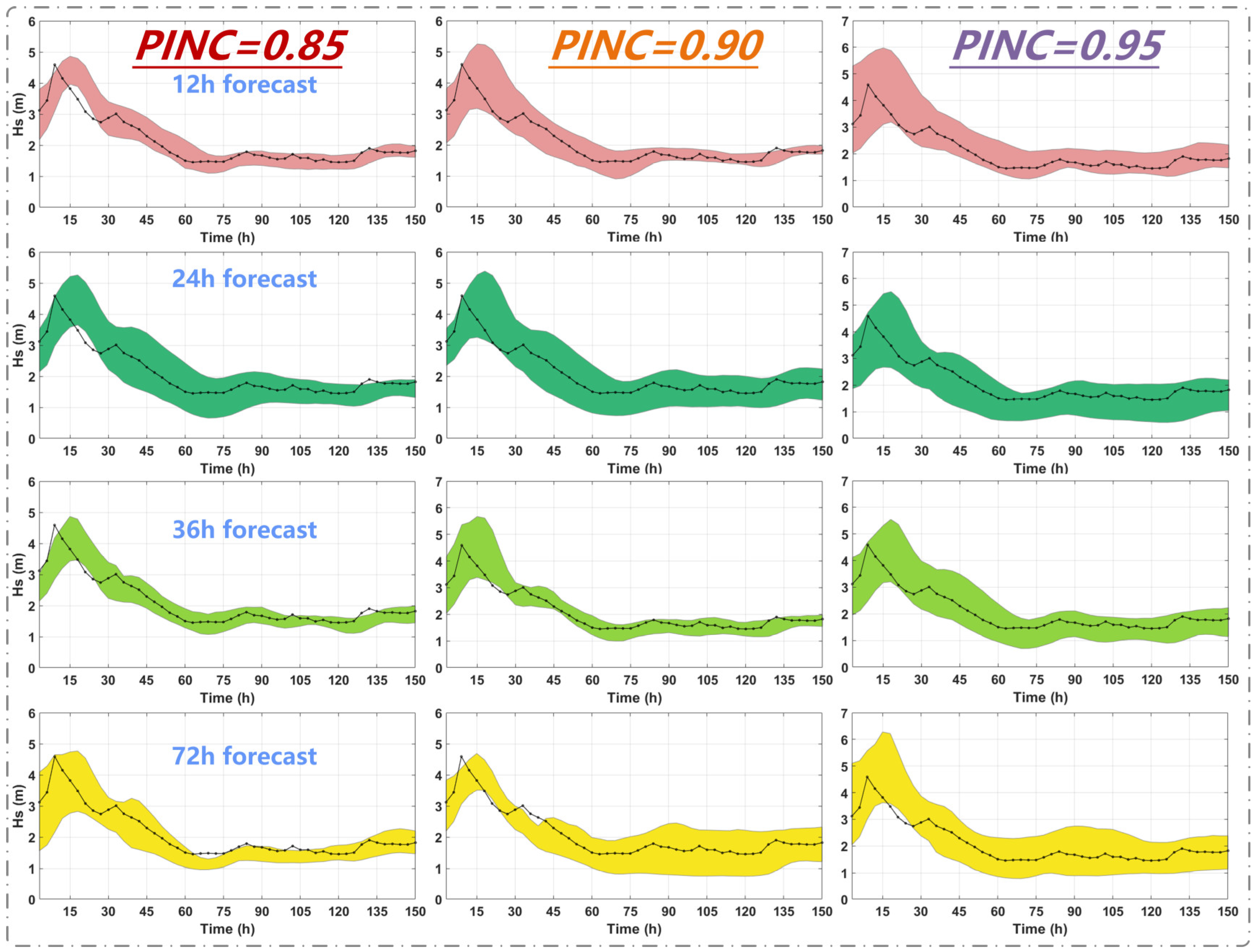
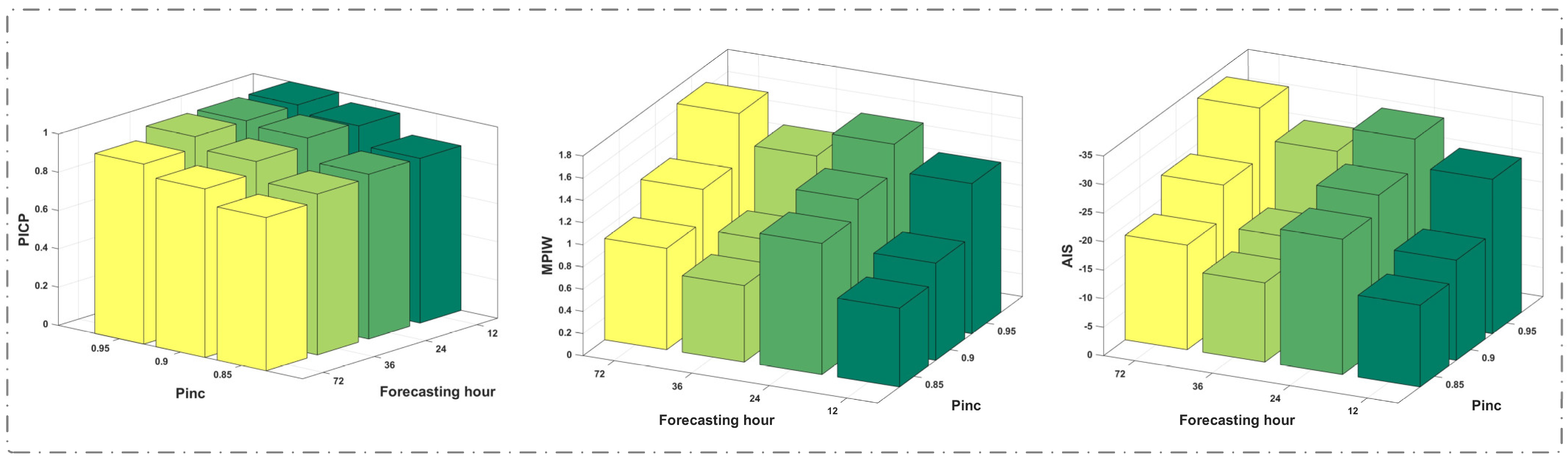
This experiment uses the dataset from the East China Sea and constant training sampling points (96 steps, 288 h in total), while varying the one-time output hours (12, 24, 36, and 72 h) to investigate the effect of various prediction hours on predictive performance. Figure 7 and Figure 8 show the visual results of interval predictions and evaluation indexes, respectively.

Figure 7 shows that, at a consistent confidence level, the coverage of interval predictions exhibits a declining trend as the prediction hour increases. In Figure 8, when PINC remains constant, it is evident that PICP progressively decreases with the growth of the prediction hours, signifying a gradual decline in the prediction level as the prediction hour increases. While the coverage rates of the 24-h forecast are not greatly distinct from that of the 36-h prediction, the MPIW and AIS suggest that the predictive quality of the 24-h forecast is worse, leading to the use of a 36-h output. Furthermore, when the output size extends to 36 h, the model still achieves effective prediction results with high coverage at a high confidence level. Figure 8 shows that when the forecasting hour is 72, the predictive performance deteriorates markedly, and at a PINC of 0.95, the complete interval coverage rate is unattainable. Consequently, we can ascertain that for multi-step forecasting of ocean wave heights, 12-, 24-, and 36-h predictions are optimal selections.

5.4. Experiment 4

In this section, enhancements in the performance of the proposed novel strategies are verified across various algorithms utilizing the single-objective test function set (CEC2005). We choose the Gray Wolf Optimizer (GWO), the Sparrow Search Algorithm (SSA), and the Gold Rush Optimization (GRO) to carry out experiments.

Table 9. Mathematical formulas of CEC2005 test functions in Experiment 4.

	Objective Function	Dim	Range	${\mathbf{F}}_{\mathbf{m}\mathbf{i}\mathbf{n}}$
F1	$f_1\left(x\right)={\sum }_{i=1}^n{x}_i^2$	30	[−100, 100]	0
F2	$f_2\left(x\right)={\sum }_{\mathsf{\Gamma }=1}^n\left|x_i\right|+{\displaystyle \prod _{i=1}^n}\left|x_i\right|$	30	[−10, 10]	0
F3	$f_3\left(x\right)={\sum }_{i=1}^n{\left({\sum }_{j=1}^i{x}_j^2\right)}^2$	30	[−100, 100]	0
F4	$f_4\left(x\right)={\mathrm{m}\mathrm{a}\mathrm{x}}_i\left\{\left|x_i\right|,1\le x_i\le n\right\}$	30	[−100, 100]	0
F5	$f_5\left(x\right)={\sum }_i^{n-1}\left[100{\left(x_{i+1}-{x_i}^2\right)}^2+{\left(x_i-1\right)}^2\right]$	30	[−30, 30]	0
F6	$f_6\left(x\right)={\sum }_{i=1}^n{\left(x_i+0.5\right)}^2$	30	[−100, 100]	0
F7	$f_7\left(x\right)={\sum }_{i=1}^{n}i{x_i}^4+\mathrm{r}\mathrm{a}\mathrm{n}\mathrm{d}\mathrm{o}\mathrm{m}\left[\mathrm{0,1}\right)$	30	[−1.28, 1.28]	0
F8	$f_8\left(x\right)=-{\sum }_{i=1}^n{x}_i\mathrm{s}\mathrm{i}\mathrm{n}\left(\sqrt{x_i}\right)$	30	[−500, 500]	−12,569.5
F9	$f_9\left(x\right)={\sum }_{i=1}^n\left[{x_i}^2-10\mathrm{c}\mathrm{o}\mathrm{s}\left(2\pi x_i\right)+10\right]$	30	[−5.12, 5.12]	0
F10	$f_{10}\left(x\right)=-20\exp \left(-0.2\sqrt{{\displaystyle \frac{1}{n}}{\displaystyle \sum _{i=1}^n}{x}_i^2}\right)-$	30	[−32, 32]	0
	$\exp \left({\displaystyle \frac{1}{n}}{\displaystyle \sum _{i=1}^n}\mathrm{c}\mathrm{o}\mathrm{s}\left(2\pi x_i\right)\right)+20+e$
F11	$f_{11}\left(x\right)={\displaystyle \frac{1}{4000}}{\sum }_{i=1}^n{x}_i^2-{\displaystyle \prod _{i=1}^n}\mathrm{c}\mathrm{o}\mathrm{s}\left({\displaystyle \frac{x_i}{\sqrt{i}}}\right)+1$	30	[−600, 600]	0

gives the mathematical formulas, and Figure 9 shows the results. The population size and evolution iteration are set consistently at 50 and 500, respectively. The results demonstrate a great enhancement in the capabilities of the three algorithms following the multi-strategy improvements.

For instance, in F1, GRO attained a maximum fitness of merely ${10}^{-70}$ after 500 iterations, whereas MSIGRO succeeded in achieving a fitness below ${10}^{-300}$, demonstrating an enhancement of over ${10}^{-230}$. For SSA, MSISSA achieved optimization in only 305 generations, resulting in an improvement of over 25%.

The search strategy of rebounding, while not augmenting computational power, notably improves the population’s capacity to avoid local optimum. In F9, the original GWO exhibits a gradual decline after 300 iterations, with the optimal fitness keeping above 1; however, the incorporation of the search strategy of rebounding brings about a decrease below ${10}^{-7}$. The above results imply that the efficiencies of algorithms obtain great improvements enhanced by the proposed strategies.

6. Summary

This paper proposes a method for short-term significant wave height prediction based on data processing and a probabilistic deep learning model, which delivers high-quality forecasts across various sea area datasets. The data processing module initially employs the hybrid mode decomposition method for denoising, greatly decreasing the non-stationarity of the original effective wave height data. By integrating the denoised data with the peak information derived from the original valid wave height data, the loss of critical information can be mitigated. The deep learning module comprises neural network layers of CNN and BiLSTM, utilizing quantile regression for probability interval prediction. Furthermore, the proposed three strategies enhance the GRO for hyperparameter optimization, improving the integration efficiency of the deep learning model, which provides wide applicability. The four research areas along the Chinese coast serve as a database, and different models are established for experimentation. Through evaluations of these models’ performance, the following conclusions can be drawn:

The application of the hybrid modal decomposition method significantly reduces the variance of the Hs sequence. Specifically, the processed results mitigate the variance of the Hs sequence with maximum reductions of 3.6% and 3%, which effectively reduces non-stationarity.

Although data denoising inevitably leads to the loss of critical information, incorporating peak information helps train deep learning models and compensates for this limitation. After applying comprehensive data processing, single models still struggle to capture both the temporal and spatial characteristics of Hs sequences and input features. In contrast, the hybrid model demonstrates stable and reliable performance in Hs prediction tasks. Furthermore, by evaluating different forecast hours, it can be found that the model ensures full interval coverage of at least a 36-h forecast at 0.95 PINC.

Nonetheless, the proposed model retains deficiencies. While our model demonstrates robust performance on unseen data within 2021–2023, its generalization to entirely unseen years (e.g., 2024 and beyond) requires further validation. This is a common challenge in data-driven wave forecasting, and we will address this limitation through extended temporal validation in future work. Although this study focuses on Chinese coastal zones due to data availability constraints, the proposed QRCNN-BiLSTM framework is designed to be generalizable to other regions. The methodology is not dependent on location-specific conditions and requires only two essential inputs for global application: significant wave height (Hs) and wave velocity data. To apply the model to global waters, we provide detailed documentation of the model architecture and training protocol in Section 3.1. Future work will systematically evaluate the model’s transferability across diverse oceanic regimes.

We plan to properly take additional factors into consideration, including the mean period of sea surface wind waves and wave direction, to enhance prediction accuracy. Future research will focus on creating more advanced and efficient models to increase practical application value.

References

1. Zheng, C.W.; Li, C.Y. Variation of the wave energy and significant wave height in the China Sea and adjacent waters. Renew. Sustain. Energy Rev. 2015, 43, 381–387. [Google Scholar] [CrossRef]
2. Ali, M.; Prasad, R. Significant wave height forecasting via an extreme learning machine model integrated with improved complete ensemble empirical mode decomposition. Renew. Sustain. Energy Rev. 2019, 104, 281–295. [Google Scholar] [CrossRef]
3. Janssen, P.A.E.M. Progress in ocean wave forecasting. J. Comput. Phys. 2008, 227, 3572–3594. [Google Scholar] [CrossRef]
4. Guedes Soares, C.; Cunha, C. Bivariate autoregressive models for the time series of significant wave height and mean period. Coast. Eng. 2000, 40, 297–311. [Google Scholar] [CrossRef]
5. Ho, P.C.; Yim, J.Z. Wave height forecasting by the transfer function model. Ocean Eng. 2006, 33, 1230–1248. [Google Scholar] [CrossRef]
6. Reikard, G.; Rogers, W.E. Forecasting ocean waves: Comparing a physics-based model with statistical models. Coast. Eng. 2011, 58, 409–416. [Google Scholar] [CrossRef]
7. Deo, M.C.; Sridhar Naidu, C. Real time wave forecasting using neural networks. Ocean Eng. 1998, 26, 191–203. [Google Scholar] [CrossRef]
8. Tian, Z.; Liu, W.; Jiang, W.; Wu, C. CNNs-Transformer based day-ahead probabilistic load forecasting for weekends with limited data availability. Energy 2024, 293, 130666. [Google Scholar] [CrossRef]
9. Deo, M.C.; Jha, A.; Chaphekar, A.S.; Ravikant, K. Neural networks for wave forecasting. Ocean Eng. 2001, 28, 889–898. [Google Scholar] [CrossRef]
10. Bazargan, H.; Bahai, H.; Aminzadeh-Gohari, A.; Bazargan, A. Neural networks based simulation of significant wave height. In Proceedings of the ASME 2007 26th International Conference on Offshore Mechanics and Arctic Engineering, San Diego, CA, USA, 10–15 June 2007; Volume 4, pp. 401–409. [Google Scholar]
11. Wang, W.; Tang, R.; Li, C.; Liu, P.; Luo, L. A BP neural network model optimized by Mind Evolutionary Algorithm for predicting the ocean wave heights. Ocean Eng. 2018, 162, 98–107. [Google Scholar] [CrossRef]
12. Bento, P.; Pombo, J.; Calado, M.d.R.; Mariano, S. Ocean wave power forecasting using convolutional neural networks. IET Renew. Power Gener. 2021, 15, 3341–3353. [Google Scholar] [CrossRef]
13. Hochreiter, S.; Schmidhuber, J. Long Short-Term Memory. Neural Comput. 1997, 9, 1735–1780. [Google Scholar] [CrossRef]
14. Jörges, C.; Berkenbrink, C.; Stumpe, B. Prediction and reconstruction of ocean wave heights based on bathymetric data using LSTM neural networks. Ocean Eng. 2021, 232, 109046. [Google Scholar] [CrossRef]
15. Pang, J.; Dong, S. A novel multivariable hybrid model to improve short and long-term significant wave height prediction. Appl. Energy 2023, 351, 121813. [Google Scholar] [CrossRef]
16. Wang, M.; Ying, F. Point and interval prediction for significant wave height based on LSTM-GRU and KDE. Ocean Eng. 2023, 289, 116247. [Google Scholar] [CrossRef]
17. Li, Q.; Wang, G.; Wu, X.; Gao, Z.; Dan, B. Arctic short-term wind speed forecasting based on CNN-LSTM model with CEEMDAN. Energy 2024, 299, 131448. [Google Scholar] [CrossRef]
18. Hao, R.; Zhao, Y.; Zhang, S.; Deng, X. Deep Learning for Ocean Forecasting: A Comprehensive Review of Methods, Applications, and Datasets. IEEE Trans. Cybern. 2025, 55, 2879–2898. [Google Scholar] [CrossRef]
19. Shen, Z.; Fan, X.; Zhang, L.; Yu, H. Wind speed prediction of unmanned sailboat based on CNN and LSTM hybrid neural network. Ocean Eng. 2022, 254, 111352. [Google Scholar] [CrossRef]
20. Dong, Z.; Tian, Z.; Lv, S. A short-term power load forecasting system based on data decomposition, deep learning and weighted linear error correction with feedback mechanism. Appl. Soft Comput. 2024, 162, 111863. [Google Scholar] [CrossRef]
21. Zhang, J.; Luo, F.; Quan, X.; Wang, Y.; Shi, J.; Shen, C.; Zhang, C. Improving wave height prediction accuracy with deep learning. Ocean Model. 2024, 188, 102312. [Google Scholar] [CrossRef]
22. Zhou, S.; Xie, W.; Lu, Y.; Wang, Y.; Zhou, Y.; Hui, N.; Dong, C. ConvLSTM-Based Wave Forecasts in the South and East China Seas. Front. Mar. Sci. 2021, 8, 1–10. [Google Scholar] [CrossRef]
23. Raj, N.; Prakash, R. Assessment and prediction of significant wave height using hybrid CNN-BiLSTM deep learning model for sustainable wave energy in Australia. Sustain. Horiz. 2024, 11, 100098. [Google Scholar] [CrossRef]
24. Scala, P.; Manno, G.; Ingrassia, E.; Ciraolo, G. Combining Conv-LSTM and wind-wave data for enhanced sea wave forecasting in the Mediterranean Sea. Ocean Eng. 2025, 326, 120917. [Google Scholar] [CrossRef]
25. Duan, W.; Huang, L. A hybrid EMD-AR model for nonlinear and non-stationary wave forecasting. J. Zhejiang Univ. Sci. A 2016, 17, 115–129. [Google Scholar] [CrossRef]
26. Hao, W.; Sun, X.; Wang, C.; Chen, H.; Huang, L. A hybrid EMD-LSTM model for non-stationary wave prediction in offshore China. Ocean Eng. 2022, 246, 110566. [Google Scholar] [CrossRef]
27. Song, T.; Wang, J.; Huo, J.; Wei, W.; Han, R.; Xu, D.; Meng, F. Prediction of significant wave height based on EEMD and deep learning. Front. Mar. Sci. 2023, 10, 1–17. [Google Scholar] [CrossRef]
28. Zhao, L.; Li, Z.; Zhang, J.; Teng, B. An Integrated Complete Ensemble Empirical Mode Decomposition with Adaptive Noise to Optimize LSTM for Significant Wave Height Forecasting. J. Mar. Sci. Eng. 2023, 11, 435. [Google Scholar] [CrossRef]
29. Tian, Z.; Gai, M. New PM2.5 forecasting system based on combined neural network and an improved multi-objective optimization algorithm: Taking the economic belt surrounding the Bohai Sea as an example. J. Clean. Prod. 2022, 375, 134048. [Google Scholar] [CrossRef]
30. Fu, W.; Fu, Y.; Li, B.; Zhang, H.; Zhang, X.; Liu, J. A compound framework incorporating improved outlier detection and correction, VMD, weight-based stacked generalization with enhanced DESMA for multi-step short-term wind speed forecasting. Appl. Energy 2023, 348, 121587. [Google Scholar] [CrossRef]
31. Ding, T.; Wu, D.; Shen, L.; Liu, Q.; Zhang, X.; Li, Y. Prediction of significant wave height using a VMD-LSTM-rolling model in the South Sea of China. Front. Mar. Sci. 2024, 11, 1–16. [Google Scholar] [CrossRef]
32. Zhang, J.; Xin, X.; Shang, Y.; Wang, Y.; Zhang, L. Nonstationary significant wave height forecasting with a hybrid VMD-CNN model. Ocean Eng. 2023, 285, 115338. [Google Scholar] [CrossRef]
33. Ding, T.; Wu, D.; Li, Y.; Shen, L.; Zhang, X. A hybrid CEEMDAN-VMD-TimesNet model for significant wave height prediction in the South Sea of China. Front. Mar. Sci. 2024, 11, 1375631. [Google Scholar] [CrossRef]
34. Zolfi, K. Gold rush optimizer: A new population-based metaheuristic algorithm. Oper. Res. Decis. 2023, 33, 113–150. [Google Scholar] [CrossRef]
35. Wang, K.; Lee, C.-H.; Juang, B.-H. Selective feature extraction via signal decomposition. IEEE Signal Process. Lett. 1997, 4, 8–11. [Google Scholar] [CrossRef]
36. Derry, A.; Krzywinski, M.; Altman, N. Convolutional neural networks. Nat. Methods 2023, 20, 1269–1270. [Google Scholar] [CrossRef]
37. Yadav, H.; Thakkar, A. NOA-LSTM: An efficient LSTM cell architecture for time series forecasting. Expert Syst. Appl. 2024, 238, 122333. [Google Scholar] [CrossRef]
38. Zhang, T.; Wang, H. Quantile regression network-based cross-domain prediction model for rolling bearing remaining useful life. Appl. Soft Comput. 2024, 159, 111649. [Google Scholar] [CrossRef]
Figure 1. Flowchart of the whole framework.
Jmse 13 01163 g001
Figure 2. Flowchart of MSIGRO.
Jmse 13 01163 g002
Figure 3. Framework of the combination neural network.
Jmse 13 01163 g003
Figure 4. IMFs of Hs of the South China Sea (x-axis: time points, y-axis: Hs).
Jmse 13 01163 g004
Figure 5. Visualization results of data denoising and augmentation.
Jmse 13 01163 g005
Figure 6. Short-term Hs forecasting results of four datasets.
Jmse 13 01163 g006
Figure 7. Results based on various forecasting hours of the East China Sea in Experiment 3.
Jmse 13 01163 g007
Figure 8. Three-dimensional view of evaluation indexes based on various forecasting hours in Experiment 3.
Jmse 13 01163 g008
Figure 9. Convergence curves of three algorithms in functions of CEC2005 in Experiment 4.
Jmse 13 01163 g009