Dynamic Frequency Optimization for Underwater Acoustic Energy Transmission: Balancing Absorption and Geometric Diffusion in Marine Environments

Abstract

The transmission efficiency of underwater acoustic is doubly constrained by absorption attenuation and geometric spreading losses, with the relative interaction between these loss mechanisms exhibiting complex dynamic variations across the frequency spectrum. Achieving dynamic equilibrium between these frequency-dependent loss mechanisms is key to enhancing acoustic energy transmission performance. To address this, this paper proposes a multi-variable coupled acoustic energy transmission model that systematically integrates the cumulative effects of the propagation distance, the geometric configuration of acoustic source arrays, and the interactive influences of critical environmental factors such as the salinity, temperature, and depth to comprehensively analyze the synergistic mechanisms of absorption loss and geometric spreading loss in practical underwater environments. Based on dynamic response analysis in the frequency dimension, the model identifies and determines the optimal working frequency ranges (i.e., dynamic equilibrium points) for maximizing the efficiency of energy transmission under various propagation conditions and environmental configurations. Both theoretical derivations and numerical simulations consistently reveal a frequency band within the low-to-mid frequency range (approximately 20–100 kHz) which is associated with significantly enhanced transmission efficiency under specific parameter settings. These research findings provide a scientific basis and engineering guidance for frequency selection and the structural optimization of underwater acoustic energy systems, offering substantial theoretical value and application prospects that can strongly support the development of acoustic technologies in ocean engineering, resource exploration, and national defense security.

1. Introduction

The underwater acoustic transfer of wireless power is one of the core topics in ocean acoustics [1,2] and is widely applied in underwater communications, ocean monitoring, resource exploration, and military technology [3,4]. By exploiting the propagation characteristics of sound waves in water, power can be supplied to submerged devices without physical contact. The basic procedure of this method is as follows: the transmitting transducer converts electrical energy into acoustic energy, the sound waves propagate through the water medium, and the receiving transducer then converts the acoustic energy back into electrical energy [5]. Compared with conventional electromagnetic induction or magnetically coupled wireless power-transfer methods, sound waves experience lower losses during underwater propagation and are immune to electromagnetic interference, enabling longer-range and more stable energy delivery [6]. Most existing studies on underwater acoustic power transfer focus only on the overall efficiency from transmission to reception, lacking an in-depth analysis of energy attenuation and sound-field distribution during the waves’ propagation and often overlooking the effects of complex underwater conditions—such as the temperature and salinity—on sound propagation [7]. Yet, the propagation stage of acoustic energy in the medium of water is crucial to the entire transfer chain, directly affecting the energy transfer efficiency and overall system performance [8]. Consequently, enhancing the efficiency of sound-wave propagation in water is regarded as a key avenue for advancing underwater acoustic power-transfer technology [9].

The transmission loss of sound waves in water is mainly composed of two parts: geometric spreading loss and medium absorption loss [10]. Absorption losses originate from molecular vibrations and chemical reactions in the medium, and their amplitude increases significantly with the frequency of the waves, especially in the high frequency range where the waves exhibit stronger energy dissipation characteristics [11]. In contrast, geometric diffusion losses are caused by the spatial distribution of energy during acoustic wave propagation and are characterized by an energy decay that is inversely proportional to the square of the propagation distance [12]. However, unlike the simple frequency dependence of absorption loss, the effect of the frequency on the geometric diffusion loss is more complex and is affected by the source layout and spatial characteristics [13].

Therefore, the frequency dependence of geometric diffusion losses needs to be analyzed in the context of the design parameters of sound source arrays used in practical applications [14]. In practical applications, array sound sources are widely used due to their controllability and strong directivity [15,16]. The directivity of the array source is closely related to the geometric diffusion loss [17], and the stronger the directivity, the smaller the geometric diffusion loss [18]. Further, the directivity of the source is affected by the number of array elements, and in general, the higher the number of array elements, the stronger the directivity [19]. However, in reality, the emitting area of an acoustic array is limited, and contained arrays need to be arranged in a specific way, so it is difficult to increase the number of arrays indefinitely in order to improve the directivity [20,21]. Therefore, the number of arrays is limited by the emission area of the source in a real application scenario [22]. In addition, the number of array elements is also affected by the spacing of the array elements [23]. In order to avoid the grating lobe effect and enhance the coherent superposition effect, the equal half-wavelength spacing design is often used in the design of actual arrays [24], where the spacing of the array elements is set as a function of the frequency and the spacing is dynamically adjusted with the change in the operating frequency. When the emitting area is fixed, the number of array elements that can be accommodated in an array with equal half-wavelength spacing increases significantly with the increasing frequency [25]. The increase in the number of array elements further enhances the directivity of the source, i.e., the spatial focusing ability of the acoustic energy is significantly increased, which reduces the geometric diffusion loss. Under the above conditions, which are consistent with real application scenarios, the geometric diffusion loss possesses a frequency dependence, where the higher the emission frequency, the lower the geometric attenuation.

At different frequencies, the relative intensity of the absorption loss and geometric spreading loss during sound wave propagation changes significantly, leading to frequency-dependent nonlinear characteristics in the efficiency of sound energy transmission [26]. Therefore, the frequency-dependent relationship between the absorption loss and geometric spreading loss constitutes a complex dynamic balance mechanism. In recent years, to investigate this mechanism, researchers have gradually begun to adopt multivariate coupling models to analyze the synergistic effects of both loss mechanisms under multiple environmental factors. Multivariate coupling models have become important tools for understanding the dynamic behavior of absorption and spreading losses under complex acoustic field conditions [27]. Through the introduction of comprehensive parameters, including frequency, propagation distance, and environmental variables such as the temperature, salinity, and depth, the research framework has been expanded from traditional single-mechanism analysis to the dynamic modeling of multi-factor interactions, which has helped to reveal the impact of dynamic balance mechanisms on the sound energy transmission efficiency in complex underwater environments and provide quantitative analytical methods for optimization.

Despite certain progress in the aforementioned research, significant deficiencies still exist in the following aspects:

First, the existing research lacks a systematic analysis of the synergistic mechanism between absorption loss and geometric spreading loss. Most studies focus on the exploration of one loss mechanism in isolation [28] or simplify the treatment of the other mechanism. For example, scholars like Zhong focused on analyzing the frequency-dependent characteristics of absorption loss [29], but ignored the dynamic changes in geometric spreading that occur under different frequency conditions; Hayrapetyan studied the influence of geometric spreading on the propagation range and directionality of sound waves, revealing their propagation characteristics in homogeneous media [30], but failed to consider the dynamic changes of absorption loss in complex underwater environments. The most common limitation of such research is the inability to effectively reveal the dynamic synergistic relationship between the two mechanisms, which results in failure to provide a systematic quantitative analysis framework to evaluate their relative contributions under different frequencies, propagation distances, and environmental conditions. In particular, there is still a lack of systematic exploration of potential dynamic balance points or optimal balance points between these two attenuation mechanisms in complex marine environments [31,32]. Additionally, the interactive influence of the sound source array configuration and environmental parameters (such as temperature, salinity, depth) on the transmission efficiency of energy has not been sufficiently emphasized [33], which has constrained the practical applicability and predictive capability of models in this field. Currently, there is no clear method available for the identification of the optimal frequency matching intervals between absorption and spreading mechanisms in practical application scenarios, nor is there engineering guidance for dynamic balance relationships.

To fill these research gaps, this paper focuses on the dynamic balance mechanism between absorption loss and geometric spreading loss, proposing an underwater sound energy transmission frequency optimization model based on their frequency-dependent synergistic effects. Specifically, this paper first analyzes the synergistic patterns of the two loss mechanisms in the frequency dimension, highlighting their effects as the propagation distance changes and providing theoretical support for an in-depth understanding of their dynamic balance mechanism. Second, this paper introduces the concept of a “dynamic balance point” and explores dynamic balance points in different underwater environmental scenarios. Additionally, this paper comprehensively considers the cumulative effects of the propagation distance, sound source array structure, and interactive impacts of key environmental variables such as the salinity, temperature, and depth, establishing a multidimensional analysis framework. This framework can identify optimal working frequency ranges that achieve the best sound energy transmission efficiency in specific environmental scenarios and for specific array configurations, and thus provides a theoretical basis for the design and optimization of underwater acoustic systems.

In summary, this research not only deepens the understanding of underwater sound energy transmission mechanisms but also provides strong theoretical support and engineering guidance for system design optimization in key application scenarios such as underwater communication, resource exploration, and military acoustics.

2. Methods

2.1. Energy Loss Modeling

The primary objective of this study is to investigate the dynamic balance between absorption loss and geometric spreading loss in underwater acoustic power transmission and, on this basis, to determine the optimal frequency band that yields the highest transmission efficiency. To eliminate the influence of external variables, the model assumes ideal transducers. This approach offers two advantages: first, it allows us to focus exclusively on the propagation of acoustic waves in the medium, avoiding interference from non-ideal transducer responses regarding frequency characteristics; second, it provides general guidance for frequency selection that is not constrained by specific hardware. Although parameters such as the transducer input impedance, sensitivity, and nonlinearity will significantly affect the system’s end-to-end efficiency, these factors pertain to subsequent stages of device design and impedance matching and, therefore, fall outside the scope of this study. Regarding the propagation characteristics of acoustic waves in underwater environments, we have identified the optimal operating frequency range, and thereby provide a basis for the design and selection of transducers in practical systems. This study further indicates that the ideal resonance frequencies of the transmitting and receiving transducers should be aligned as closely as possible with the medium’s optimal propagation frequency, identified here, in order to maximize the overall end-to-end efficiency of the system.

In the process of underwater acoustic wave propagation, the loss of acoustic energy mainly includes geometric diffusion loss and medium absorption loss. Therefore, an accurate description of the energy loss mechanism of acoustic wave propagation in water is crucial for optimizing the transmission effect of acoustic waves and selecting the best frequency. To quantitatively analyze the loss mechanism of underwater acoustic wave energy, this study firstly establishes an energy loss model from the basic principle of acoustic wave propagation, which is combined with the fluctuation equation.

The theoretical framework for acoustic propagation is grounded in the classical acoustic wave equation [34]. In a homogeneous, loss-free medium, this linear wave equation couples acoustic pressure with particle velocity and can be expressed as a second-order linear partial differential equation [35,36]. A widely adopted solution strategy assumes a single-frequency, harmonic time dependence for the pressure field [37]. Substituting this assumption into the wave equation converts it to the frequency-domain Helmholtz equation [38], in which the canonical solution for a point source in an unbounded medium (free field) is [39]:

$$P\left(r\right)={\displaystyle \frac{A}{r}}{e}^{ikr}$$

(1)

where $P\left(r\right)$ denotes the spatial distribution of acoustic pressure; $k$ is the wavenumber; $A$ is the initial sound-pressure amplitude; $r$ is the distance from the point source to the observation point; and $e^{ikr}$ represents the propagation of a spherical wave. This frequency-domain representation describes steady-state sound propagation at a specified frequency, and the resulting solution yields the spatial distribution of acoustic pressure [40]. For a point source, the solution manifests as a spherical wave in which the pressure amplitude decays proportionally to 1/r with distance, reflecting the geometric spreading of acoustic energy over ever-increasing spherical surfaces [41].

To isolate and examine the acoustic energy loss induced by geometric spreading, the preceding theoretical derivation, which is based on an idealized linear wave equation, can be used, assuming a propagation medium free of energy dissipation. However, in realistic ocean environments, acoustic waves in water are inevitably subjected to medium absorption and frequency-dependent attenuation, which results in a progressive decrease in the acoustic pressure amplitude with distance. In response, this study develops a more realistic underwater acoustic energy propagation model that extends the idealized framework by incorporating both frequency-dependent absorption effects and geometric spreading losses associated with source array-induced spatial heterogeneity in the marine environment. This enhanced model aims to more accurately characterize the actual propagation behavior of acoustic energy in seawater.

2.2. Geometric Diffusion and Absorption Loss Modeling

2.2.1. Modeling Geometric Diffusion Losses

Equation (1), the Helmholtz equation, is based on a spherical wave source, i.e., an omnidirectional sound field that produces a uniform distribution of acoustic energy. Its geometric diffusion loss is a volume effect in a single distance dimension and manifests itself as a sound intensity attenuation of $1/r^2$.

The array of sound sources can form a multi-point, even directional sound field, which can reflect the non-uniformity of the sound field in space; the superposition of its multiple sources can simulate the acoustic interactions in different regions (e.g., coherent and incoherent superposition), which can further reveal the effect of spatial heterogeneity on the distribution of acoustic energy [5]. In addition, the array can control the propagation of acoustic waves in a specific direction and analyze the geometric diffusion characteristics of acoustic energy propagating with different paths. Therefore, the array model is adopted to reflect the spatial heterogeneity and combined with the solution of the Helmholtz equation to further investigate the relationship between geometric diffusion loss and spatial location, and the resulting model more realistically reflects the acoustic energy distribution characteristics in complex environments.

It is assumed that the linear array consists of $N$ equally spaced point sources with a total length of $L$. According to the principle of avoiding grating lobes, the array element spacing $d$ should be satisfied in order to obtain the best beam directivity:

$$d={\displaystyle \frac{\lambda }{2}}={\displaystyle \frac{c}{2f}}$$

(2)

where $\lambda$ is the wavelength; $c$ is the speed of sound; $f$ is the frequency of the sound wave. For a linear array, the total length of the array $L$ is related to the number of array elements $N$ and the spacing of the elements $d$:

$$L=\left(N-1\right)d=\left(N-1\right){\displaystyle \frac{\lambda }{2}}$$

(3)

Solve for $N$:

$$N={\displaystyle \frac{2L}{\lambda }}+1={\displaystyle \frac{2Lf}{c}}+1$$

(4)

Here, we get a more precise expression where $N$ must be an integer.

The following are considerations of integer properties:

Exact value: $N=⌈{\displaystyle \frac{2L}{\lambda }}+1⌉$ where ⌈ ⌉ means round down.

Approximation: when $N$ is very large, the effect of $+1$ is relatively small and can be ignored, but for the smaller $N$, it must be calculated precisely.

In an array of multiple sources, the sound pressure equation for the sound field is relatively complicated because the interference of multiple sources affects the sound field distribution. Based on the principle of linear superposition of the Helmholtz equation, the sound pressure of the array $p(r,\theta )$ can be expressed as follows:

$$p\left(r,\theta \right)=\sum _{n=1}^N {\displaystyle \frac{A_n{e}^{ik{R}_n}}{R_n}}$$

(5)

where $A_n=A$ is the amplitude of the first $n$ source (assuming that all array elements are equal in amplitude), $r$ is the distance of the receive position from the center of the array (the origin), $\theta$ is the angle of the receive position with respect to the center of the array, and $R_n$ is the distance of the receive position from the $n$th array element. If the array lies on the $x$-axis, the coordinates of the $n$th array element are $\left(x_n, 0\right)$, where $x_n=(N-1)d$. Therefore, the distance from the receiving position to the $n$th array element $R_n$ can be expressed as follows:

$$R_n=\sqrt{{\left(\mathrm{rcos}\theta -x_n\right)}^2+{\left(\mathrm{rsin}\theta \right)}^2}$$

(6)

Substituting the expression for ${\pm R}_n$ into the sound pressure Equation (5) gives:

$$p\left(r,\theta \right)=\sum _{n=1}^N {\displaystyle \frac{A{e}^{ik\sqrt{(\mathrm{rcos}\theta -x_n{)}^2+(\mathrm{rsin}\theta {)}^2}}}{\sqrt{(\mathrm{rcos}\theta -x_n{)}^2+(\mathrm{rsin}\theta {)}^2}}}$$

(7)

Equation (8) represents the far-field approximation of the acoustic pressure field, which is derived under the assumption that the observation point is sufficiently distant from the sound source (${\displaystyle \frac{L^2}{\lambda }}$), allowing simplifications based on the Fraunhofer approximation [42].

$$p\left(r,\theta \right)\approx {\displaystyle \frac{A{e}^{ikr}}{r}}\sum _{n=1}^N e^{-ik{x}_n\cos \theta }$$

(8)

The summation term for the angle $\theta$ is called the directionality factor $D(\theta )$:

$$D\left(\theta \right)=\sum _{n=1}^N e^{-ik{x}_n\cos \theta }$$

(9)

Substituting $x_n$ for the equally spaced, half-wavelength-distributed linear arrays studied in this paper, the geometric progression can be obtained by solving the following:

$$D\left(\theta \right)={\displaystyle \frac{\sin \left(N\frac{\pi }{2}\cos \theta \right)}{\sin \left(\frac{\pi }{2}\cos \theta \right)}}$$

(10)

The numerator term reflects the directional primary and secondary flap distributions of the array, and the denominator term reflects the fluctuating interference due to the spacing between the sources [43].

Substituting the directionality factor, the sound pressure of the array can be expressed as follows:

$$p\left(r,\theta \right)={\displaystyle \frac{A{e}^{ikr}}{r}}D\left(\theta \right)$$

(11)

2.2.2. Modeling Underwater Acoustic Energy Absorption Losses

Seawater is a dissipative propagation medium, and dissipation is primarily caused by the viscosity or chemical reaction of the medium. The main model used nowadays is the Francois–Garrison model, which is a classical underwater acoustic absorption loss model that is widely used in ocean acoustics to characterize the propagation and absorption of acoustic waves in seawater [44]. The model decomposes the sources of the acoustic absorption coefficient, including the contributions of boric acid, magnesium sulfate, and pure water.

The absorption coefficient is decomposed into three terms that correspond to the roles of boric acid, magnesium sulfate, and pure water:

$$\alpha =A_1{P}_1{\displaystyle \frac{f_1{f}^2}{f_1^2+f^2}}+A_2{P}_2{\displaystyle \frac{f_2{f}^2}{f_2^2+f^2}}+A_3{P}_3{f}^2$$

(12)

Role of boric acid [${\mathrm{B}(\mathrm{O}\mathrm{H})}_3$].

$$\left\{\begin{array}{l}{A}_1={\displaystyle \frac{8.86}{c}}{10}^{\left(0.78pH-5\right)}\\ P_1=1\\ f_1=2.8\sqrt{{\displaystyle \frac{S}{35}}}{10}^{\left(4-\frac{1245}{7+273}\right]}\\ c=1412+3.21T+1.19S+0.0167z\end{array}\right.$$

(13)

Magnesium sulfate (${\mathrm{M}\mathrm{g}\mathrm{S}0}_4$).

$$\left\{\begin{array}{l}{A}_2=21.44{\displaystyle \frac{S}{c}}(1+0.025T)\\ P_2=1-1.37\times {10}^{-4}z+6.2\times {10}^{-9}{z}^2\\ f_2={\displaystyle \frac{8.17\times {10}^{\left[8-\frac{1990}{T+273}\right]}}{1+0.0018\left(S-35\right)}}\end{array}\right.$$

(14)

The role of pure water viscosity.

$$\left\{\begin{array}{l}{P}_3=1-3.83\times {10}^{-5}z+4.9\times {10}^{-10}{z}^2\\ A_3=4.937\times {10}^{-4}-2.59\times {10}^{-5}T+9.11\times {10}^{-7}{T}^2-1.5\times {10}^{-8}{T}^3, T\le 20 °\mathrm{C}\\ A_3=3.964\times {10}^{-4}-1.146\times {10}^{-5}T+1.45\times {10}^{-7}{T}^2-6.5\times {10}^{-8}{T}^3, T>20 °\mathrm{C}\end{array}\right.$$

(15)

In the above formula, $\alpha$ is the absorption coefficient, in dB/km; z is the depth, in m; S is the salinity, in psu (actual salinity unit); T is the temperature, in °C; pH is the acidity; $f$ is the acoustic frequency, in kHz; A1, A2, and A3 are empirical amplitude coefficients corresponding to the absorption mechanisms of boric acid, magnesium sulfate, and viscous pure water, respectively. $P_1$, $P_2$, and $P_3$ are depth-correction factors that account for the variation of sound pressure with depth. $f_1$ and $f_2$ denote the relaxation frequencies characteristic of boric acid and magnesium sulfate, respectively (kHz).

In the process of underwater acoustic wave propagation, the presence of the medium’s viscosity and chemical reactions inevitably leads to absorption attenuation of the acoustic energy. This absorption loss typically manifests as an exponential decline in the acoustic pressure amplitude with an increasing propagation distance and can be quantitatively described by introducing an exponential decay function with the absorption attenuation coefficient $\alpha$ as a parameter. Specifically, when a sound wave travels a distance $r$ in an underwater medium, the pressure amplitude $p(r)$, considering the medium absorption loss, can be expressed as follows:

$$p\left(r\right)=A{e}^{-\alpha r}$$

(16)

This exponential attenuation expression clearly reveals the quantitative relationship between the absorption loss and propagation distance in underwater media, serving as an important theoretical foundation for further analysis and optimization of acoustic energy transmission efficiency.

2.3. Establishing Quantitative Trade-Offs Between Geometric Diffusion and Absorption Loss Modeling

By combining the underwater acoustic absorption loss model with the geometric diffusion loss model, a complete mathematical expression for the attenuation of the acoustic field can be obtained. At this point, the overall attenuation includes the geometric diffusion loss and medium absorption loss.

The corrected formula for the sound pressure $p(r,\theta )$, taking geometric spreading and absorption losses into account, is expressed as follows:

$$p\left(r,\theta \right)=A\cdot {\displaystyle \frac{e^{-\alpha r}}{r}}\cdot D\left(\theta \right)$$

(17)

Equation (11) includes the term $e^{ikr}$, representing a periodic spatial and temporal variation in the acoustic wave phase as it propagates through the medium. While this term is mathematically expressed using an imaginary exponent, it carries clear physical significance, describing the progressive phase shift of the wavefronts rather than directly affecting the amplitude attenuation. In the context of analyzing geometric diffusion and absorption losses, our primary interest lies in the amplitude variations in the acoustic pressure field. Therefore, the explicit consideration of phase variations, although physically meaningful for wave propagation analysis, does not impact the amplitude-based attenuation evaluation in this study and is consequently omitted from further discussion.

Sound intensity $I(r,\theta )$ is defined as the sound power per unit area (energy flow density), and is proportional to the square of the sound pressure [45]:

$$I\left(r,\theta \right)={\displaystyle \frac{|p(r,\theta ){|}^2}{\rho c}}$$

(18)

where $\rho$ is the density of the medium.

Substituting Equation (17), the final mathematical expression for the sound intensity is expressed as follows:

$$I(r,\theta )={\displaystyle \frac{A^2}{\rho c{r}^2}}{e}^{-2\alpha r}|D\left(\theta \right){|}^2$$

(19)

This equation describes the sound intensity at an underwater sound propagation distance of $r$ and a reception angle of $\theta$, taking into account the directionality of the array (via the array factor $D(\theta )$), the propagation loss (attenuating with $r^2$), i.e., the geometric diffusion loss, and the absorption attenuation (expressed via $e^{-2\alpha r}$).

Sound power $W$ is the total power of a sound wave passing over a closed surface and can be obtained by integrating the sound intensity:

$$W={\int }_S I\left(r,\theta \right)dS$$

(20)

where $S$ is a sphere or other closed surface.

In practical acoustic applications, it may be necessary to integrate the entire closed surface or a portion of a region in a specific direction to obtain the total sound power or the sound power in a specific direction. The exact range of integration depends on the characteristics of the source and the location of the receiving point.

The object of the sound field analysis in this study is a linear array sound source. The distribution of its radiated sound energy in space shows obvious axial symmetry. The directivity factor $D(\theta )$ of the array is usually only reflected by the distribution law of the angle θ along the array axis and does not depend on the azimuth angle $\varphi$ around the array axis [43].

At the receiving position $(r,\theta )$, the acoustic power received by the tiny area element on the receiving surface $dS$ depends partially on the effects of underwater acoustic absorption and geometric diffusion:

$$dS=r^2\sin \theta d\theta d\varphi$$

(21)

Under axial symmetry conditions, the sound intensity value at any fixed $\varphi$ on the sphere is uniformly distributed along the $\varphi$ direction. Therefore, the closed integral over the sphere can be decomposed into the following:

$$W={\int }_S I\left(r,\theta \right)dS={\int }_0^{2\pi } {\int }_0^{\pi } I(r,\theta )r^2\mathrm{s}\mathrm{i}\mathrm{n}\theta d\theta d\varphi =2\pi {\int }_0^{\pi } I(r,\theta )r^2\sin \theta d\theta$$

(22)

The local sound power $W_{\mathrm{r}\mathrm{e}\mathrm{c}\mathrm{e}\mathrm{i}\mathrm{v}\mathrm{e}\mathrm{d}}(r,\theta )$ is obtained by integrating the sound intensity $I(r,\theta )$ over the receiving area. If the receiving area is a small spherical crown (area limited to a specific direction $\theta \in [{\theta }_1,{\theta }_2]$), the integral is expressed as follows:

$$W_{\mathrm{r}\mathrm{e}\mathrm{c}\mathrm{e}\mathrm{i}\mathrm{v}\mathrm{e}\mathrm{d}}\left(r,\theta \right)=2\pi {\int }_{{\theta }_1}^{{\theta }_2} I\left(r,\theta \right)r^2\sin \theta d\theta$$

(23)

Substitute the sound intensity Equation (23):

$$W_{\mathrm{r}\mathrm{e}\mathrm{c}\mathrm{e}\mathrm{i}\mathrm{v}\mathrm{e}\mathrm{d}}(r,\theta )=2\pi {\displaystyle \frac{A^2}{\rho c}}{e}^{-2\alpha r}{\int }_{{\theta }_1}^{{\theta }_2} |D(\theta ){|}^2\sin \theta d\theta$$

(24)

The total sound power of the source $W_{\mathrm{t}\mathrm{o}\mathrm{t}\mathrm{a}\mathrm{l}}$ is the power of the source on the sphere when it is not affected by absorption losses, i.e., it does not include $e^{-2\alpha r}$. At this time, the sound intensity is expressed as follows:

$$I_{\mathrm{n}\mathrm{o}\mathrm{l}\mathrm{o}\mathrm{s}\mathrm{s}}(r,\theta )={\displaystyle \frac{A^2}{\rho c{r}^2}}|D(\theta ){|}^2$$

(25)

Integral sound power is expressed as follows:

$$W_{\mathrm{t}\mathrm{o}\mathrm{t}\mathrm{a}\mathrm{l}}=2\pi {\int }_0^{\pi } I_{\mathrm{n}\mathrm{o}\mathrm{l}\mathrm{o}\mathrm{s}\mathrm{s}}\left(r,\theta \right)r^2\sin \theta d\theta$$

(26)

Simplification is expressed as follows:

$$W_{\mathrm{t}\mathrm{o}\mathrm{t}\mathrm{a}\mathrm{l}}=2\pi {\displaystyle \frac{A^2}{\rho c}}{\int }_0^{\pi } {\left|D\left(\theta \right)\right|}^2\sin \theta d\theta$$

(27)

Transmission efficiency is defined as the ratio of received position power to total power:

$$\eta \left(r,\theta \right)={\displaystyle \frac{W_{\mathrm{r}\mathrm{e}\mathrm{c}\mathrm{e}\mathrm{i}\mathrm{v}\mathrm{e}\mathrm{d}}\left(r,\theta \right)}{W_{\mathrm{t}\mathrm{o}\mathrm{t}\mathrm{a}\mathrm{l}}}}$$

(28)

Substitute $W_{\mathrm{r}\mathrm{e}\mathrm{c}\mathrm{e}\mathrm{i}\mathrm{v}\mathrm{e}\mathrm{d}}(r,\theta )$ and $W_{\mathrm{t}\mathrm{o}\mathrm{t}\mathrm{a}\mathrm{l}}$:

$$\eta \left(r,\theta \right)={\displaystyle \frac{2\pi \frac{A^2}{\rho c}{e}^{-2\alpha r}{\int }_{{\theta }_1}^{{\theta }_2} |D(\theta ){|}^2\sin \theta d\theta }{2\pi \frac{A^2}{\rho c}{\int }_0^{\pi } |D(\theta ){|}^2\sin \theta d\theta }}$$

(29)

After simplification, the transmission efficiency equation is expressed as follows:

$$\eta \left(r,\theta \right)=e^{-2\alpha r}\cdot {\displaystyle \frac{{\int }_{{\theta }_1}^{{\theta }_2} |D\left(\theta \right){|}^2\sin \theta d\theta }{{\int }_0^{\pi } |D\left(\theta \right){|}^2\sin \theta d\theta }}$$

(30)

Transmission efficiency consists of two parts:

The absorption attenuation term $e^{-2\alpha r}$ describes the loss of energy due to the absorption of the sound wave over the propagation distance $r$, which decays exponentially.

Directional factor integral ratio is expressed as follows:

$${\displaystyle \frac{{\int }_{{\theta }_1}^{{\theta }_2} |D\left(\theta \right){|}^2\sin \theta d\theta }{{\int }_0^{\pi } |D\left(\theta \right){|}^2\sin \theta d\theta }}$$

(31)

The numerator describes the cumulative power of the directionality factor of the sound field over the reception area (${\theta }_1,{\theta }_2$). The denominator describes the total directional factor power over the entire sphere.

If the reception area is a small area in a specific direction, then (${\theta }_1,{\theta }_2$) is very narrow, and this results in a small integration ratio, indicating a low reception efficiency. If the receiving region extends over the entire sphere, the integral ratio is 1 and the transmission efficiency degrades to $e^{-2\alpha r}$.

This equation accurately describes the combined effect of the absorption loss and directionality factor on the efficiency of acoustic energy transfer in a specific direction for the propagation distance $r$ and the specific direction (${\theta }_1,{\theta }_2$).

In this study, acoustic power efficiency is adopted as the primary performance metric for assessing energy transfer, as it directly quantifies the balance between geometric spreading and absorption losses under dynamic environmental conditions. Although sound pressure level (SPL) beam patterns are widely used for beamforming analysis, they focus mainly on spatial directivity and beam structure and may fail to capture the cumulative energy distribution over the propagation distance or the frequency-dependent absorption effects encountered in complex underwater environments [5].

Specifically, Equation (31) integrates the directivity factor and weights the directivity function $|D\left(\theta \right){|}^2$ over the reception angular range, and thereby inherently accounts for the spatial distribution of energy. This approach avoids the oversimplification that results from relying solely on SPL-based beam patterns and prevents the spatial heterogeneity of absorption and geometric spreading losses from being overlooked.

2.4. Optimal Frequency Solution

The absorption loss terms $e^{-2\alpha (f)r}$, $\alpha (f)$ are known to be functions of frequency (the frequency-dependent absorption coefficients given in the Francois–Garrison model). $|D(f,\theta ){|}^2$: the square of the directionality factor, related to the frequency $f$.

Analyze the solution of the optimal frequency:

(1) Frequency dependence of $\alpha (f)$

Absorption coefficients $\alpha (f)$ usually have a complex frequency dependence (e.g., the Francois–Garrison model) and require a specific form for numerical calculations. Typical properties include the following: The absorption coefficient increases significantly with the frequency in certain frequency ranges. The acoustic energy transfer efficiency shows a significant decrease with increasing frequency.

(2) Frequency dependence of $D(f,\theta )$

The directionality factor $|D(f,\theta ){|}^2$ is frequency dependent, especially at high frequencies, where directional effects are more concentrated and may lead to an increase in transmission efficiency compared to lower frequencies.

In order to find the optimal frequency $f_{opt}$ to maximize the efficiency $\eta$, we need to take the derivative of the efficiency equation $\eta$ with respect to the frequency $f$ and set its derivative to zero.

The transmission efficiency equation can be expressed as the product of two terms:

$$\eta \left(r,\theta \right)=\underset{\mathrm{Absorption} \mathrm{term}}{\underbrace{e^{-2\alpha \left(f\right)r}}}\cdot \underset{\mathrm{Directional} \mathrm{factor} \mathrm{term}}{\underbrace{{\displaystyle \frac{{\int }_{{\theta }_1}^{{\theta }_2} |D\left(f,\theta \right){|}^2\sin \theta d\theta }{{\int }_0^{\pi } |D\left(f,\theta \right){|}^2\sin \theta d\theta }}}}$$

(32)

Remember the following:

$$\eta \left(r,\theta \right)=e^{-2\alpha \left(f\right)r}\cdot G\left(f\right)$$

(33)

where $G(f)$ denotes the normalized effect of the directionality factor on the frequency $f$:

$$G\left(f\right)={\displaystyle \frac{{\int }_{{\theta }_1}^{{\theta }_2} |D\left(f,\theta \right){|}^2\sin \theta d\theta }{{\int }_0^{\pi } |D\left(f,\theta \right){|}^2\sin \theta d\theta }}$$

(34)

Find the derivative of $\eta (r,\theta )$ with respect to $f$ and use the product rule:

$${\displaystyle \frac{\partial \eta \left(r,\theta \right)}{\partial f}}=\underset{\mathrm{Derivative} \mathrm{of} \mathrm{the} \mathrm{absorption} \mathrm{term}}{\underbrace{{\displaystyle \frac{\partial }{\partial f}}\left[e^{-2\alpha \left(f\right)r}\right]}}\cdot G\left(f\right)+e^{-2\alpha \left(f\right)r}\cdot \underset{\mathrm{Derivative} \mathrm{of} \mathrm{Directivity} \mathrm{Factor}}{\underbrace{{\displaystyle \frac{\partial G\left(f\right)}{\partial f}}}}$$

(35)

The derivative of the absorption term $e^{-2\alpha (f)r}$ is expressed as follows:

$${\displaystyle \frac{\partial }{\partial f}}\left[\begin{array}{c}{e}^{-2\alpha \left(f\right)r}\end{array}\right]=-2r\cdot e^{-2\alpha \left(f\right)r}\cdot {\displaystyle \frac{\partial \alpha \left(f\right)}{\partial f}}$$

(36)

The derivative of the directionality factor $G(f)$ is expressed as follows:

$${\displaystyle \frac{\partial G\left(f\right)}{\partial f}}={\displaystyle \frac{\frac{\partial }{\partial f}{\int }_{{\theta }_1}^{{\theta }_2} |D\left(f,\theta \right){|}^2\sin \theta d\theta }{{\int }_0^{\pi } |D\left(f,\theta \right){|}^2\sin \theta d\theta }}-G\left(f\right)\cdot {\displaystyle \frac{\frac{\partial }{\partial f}{\int }_0^{\pi } |D\left(f,\theta \right){|}^2\sin \theta d\theta }{{\int }_0^{\pi } |D\left(f,\theta \right){|}^2\sin \theta d\theta }}$$

(37)

Set the total derivative to zero:

$$\begin{array}{c}-2r\cdot e^{-2\alpha \left(f\right)r}\cdot {\displaystyle \frac{\partial \alpha \left(f\right)}{\partial f}}\cdot G\left(f\right)+e^{-2\alpha \left(f\right)r}\cdot {\displaystyle \frac{\partial G\left(f\right)}{\partial f}}=0\end{array}$$

(38)

After simplification, the equation is expressed as follows:

$${\displaystyle \frac{\partial G\left(f\right)}{\partial f}}=2r\cdot G\left(f\right)\cdot {\displaystyle \frac{\partial \alpha \left(f\right)}{\partial f}}$$

(39)

Since these formulas involve complex integral terms and nonlinear relationships, numerical optimization methods (e.g., Newton’s method) are often required to determine the optimal frequency [46].

In order to apply Newton’s method, we also need $g^{\prime }(f)$ (i.e., ${\displaystyle \frac{{\partial }^2\eta (f)}{\partial f^2}}$), but due to its complexity, it is usually computed numerically. The iterative formula for Newton’s method is expressed as follows:

$$f_{n+1}=f_n-{\displaystyle \frac{g\left(f_n\right)}{g^{\prime }\left(f_n\right)}}$$

(40)

where, in this problem, the derivative of the transmission efficiency is the objective function $g(f_n)$:

$$g\left(f_n\right)=e^{-2\alpha \left(f_n\right)r}\cdot {\displaystyle \frac{\partial G\left(f_n\right)}{\partial f}}-2r\cdot e^{-2\alpha \left(f_n\right)r}\cdot G\left(f_n\right)\cdot {\displaystyle \frac{\partial \alpha \left(f_n\right)}{\partial f}}$$

(41)

$g^{\prime }(f_n)$ is the derivative of $g(f_n)$:

$$g^{\prime }\left(f_n\right)={\displaystyle \frac{{\partial }^2\eta \left(f\right)}{\partial f^2}}$$

(42)

The second-order derivative of the transmission efficiency function $g(f)$ with respect to the frequency $f$ can be obtained through analytical derivation:

$$g^{\prime }\left(f_n\right)\approx {\displaystyle \frac{g\left(f_n+\mathsf{\Delta }f\right)-g\left(f_n\right)}{\mathsf{\Delta }f}}$$

(43)

However, due to its nonlinear characteristics and complex integral terms, the analytical expression becomes very complicated. Therefore, for simplicity and efficiency in calculation, numerical differentiation methods are adopted to approximate the second-order derivative. The flowchart for the frequency optimization method based on the underwater sound absorption loss and geometric diffusion attenuation model is shown in Figure 1:

3. Results and Discussion

3.1. Experimental Setup

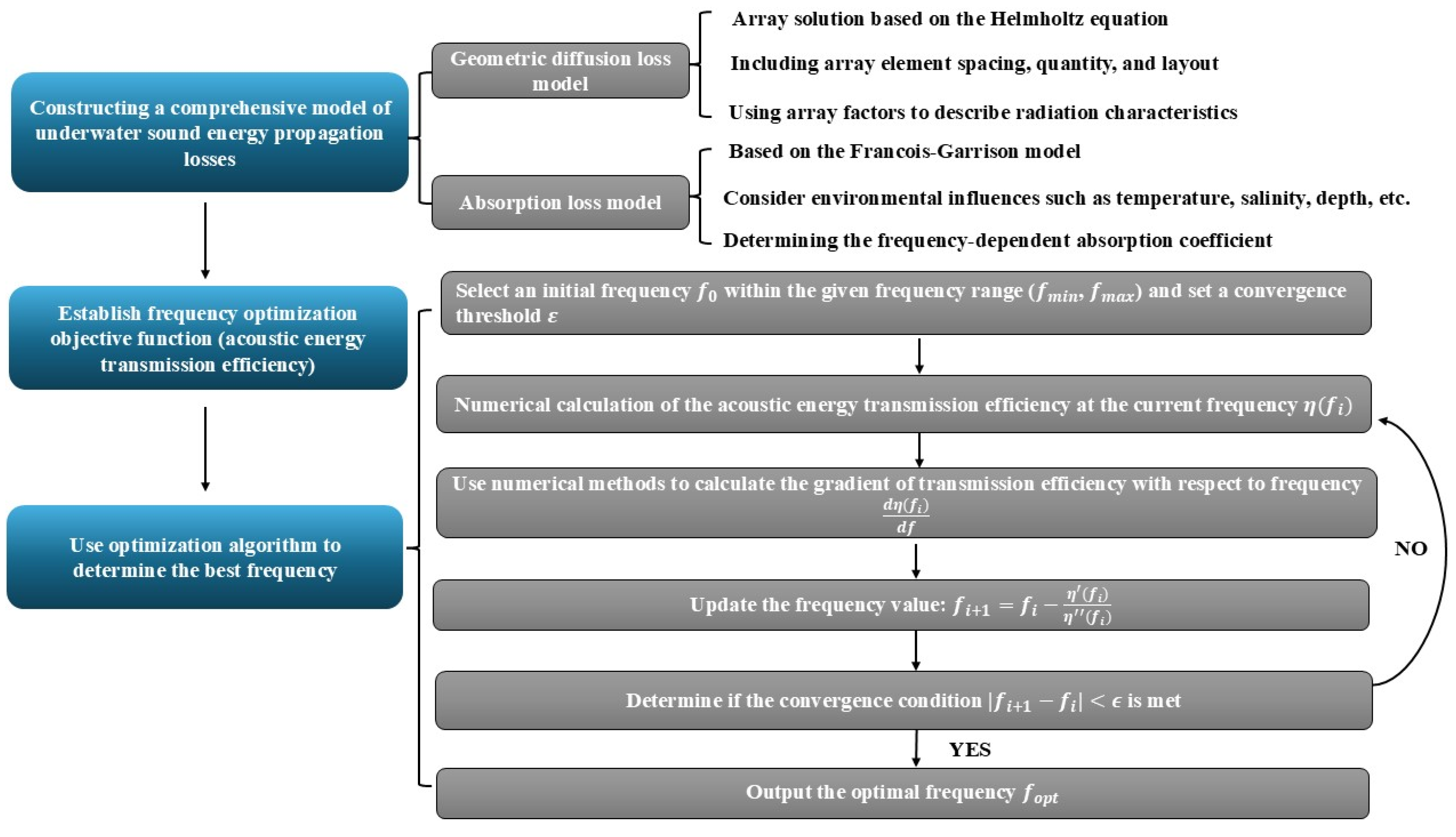
In the practical application of underwater acoustic systems, it is often necessary to complete the layout design of the acoustic source array according to the design requirements of the real underwater environment application scenario. Therefore, this paper investigates the frequency optimization compensation method for determining the underwater acoustic energy transmission loss under multiple constraints of array layout parameters and underwater environment parameters.

3.1.1. Experimental Parameter Setting

Array geometry parameters: In this study, array geometry parameters were systematically established for different acoustic array configurations. The overall physical dimension of the transmitting array was initially fixed by design constraints associated with the intended application scenario. However, the spacing between individual array elements was defined as half of the acoustic wavelength corresponding to the chosen operating frequency. This half-wavelength element spacing was deliberately selected to minimize the occurrence of grating lobes, maximize the coherent constructive interference, and effectively suppress unwanted diffraction effects. Consequently, although the physical boundary of the array was fixed, the actual number of array elements and layers varied dynamically with the operating frequency due to the inverse proportionality between the wavelength and frequency. Specifically, higher operating frequencies result in smaller wavelengths, allowing a larger number of elements to be integrated within the fixed array dimensions and thereby enhancing the array’s directional performance.

The linear array lengths were set to 0.75 m and 0.5 m, reflecting typical dimensions of underwater acoustic transmitting arrays. The 0.75 m length was chosen to represent a relatively large yet practical aperture for underwater applications—roughly the maximum size that can be mounted on an underwater vehicle or a moored system without becoming unwieldy. The 0.5 m length, by contrast, represents a compact array design. This dimension is common in portable or space-constrained underwater equipment and allows us to examine the performance trade-offs associated with a reduced aperture. Using a 0.5 m array therefore allows us to model scenarios in which physical space is limited, a situation frequently encountered by small autonomous underwater vehicles or seabed instruments in practice.

Operating frequency range: Moreover, different frequency ranges were deliberately selected for various array configurations (linear, equidistant hexagonal, and circular arrays) to evaluate their performance under distinct operational conditions—low-frequency scenarios emphasize deeper penetration despite higher absorption losses, whereas high-frequency scenarios offer increased spatial resolution at the cost of a reduced penetration capability. To effectively quantify the impact of the frequency on the acoustic transmission performance, frequency sweeps were conducted with frequency resolutions that differed by 1 kHz increments, spanning the entire experimental frequency range listed in

Table 1. Experimental frequency range and array geometry parameters used for different arrays.

	Frequency Range	Array Size	Element Spacing
Linear array	1–300 kHz	0.75 m & 0.5 m	Half-wavelength
Equidistant hexagonal array	1–200 kHz	0.25 m (Radius)	Half-wavelength
Circular array	1–200 kHz	0.25 m (Radius)	Half-wavelength

. This chosen resolution ensures sufficient granularity for accurately capturing variations in acoustic propagation efficiency and adequately supports subsequent optimization analysis.

For the line array, we extended the frequency sweep to 300 kHz. This higher ceiling allowed us to investigate the high-frequency region where the array’s directivity could markedly enhance the efficiency—and to assess the point at which the absorption losses negate those gains. Even at 300 kHz, the computational burden for the line array was still manageable, so we kept the entire sweep range to capture any potential ultra-high-frequency efficiency peaks.

For the planar arrays (hexagonal and circular), the sweep was capped at 200 kHz. Beyond roughly 200 kHz, the absorption in water becomes so severe that the long-range transmission efficiency approaches zero, and modeling two-dimensional arrays in this band would demand an extremely fine spatial mesh with a prohibitive computational cost. In practice, most underwater acoustic power systems also operate below 200 kHz, so this upper limit is well-justified on both physical and computational grounds.

These frequency-domain simulations effectively treat the source excitation as a steady-state continuous wave at each discrete frequency. Our study focuses on identifying the dynamic equilibrium frequency that maximizes the transmission efficiency of underwater acoustic energy by balancing geometric spreading and absorption losses. To achieve this, we employed continuous sinusoidal signals (frequency sweeps) rather than impulse excitation, for the following reasons:

Frequency-dependent optimization: Continuous excitation allows us to conduct systematic frequency sweeps (1 kHz resolution) to evaluate the transmission efficiency across a broad spectrum. This approach directly aligns with our goal of identifying optimal frequency ranges where the absorption and geometric diffusion losses dynamically balance.

Steady-state energy metrics: impulse excitation primarily captures transient time-domain responses, which are less relevant for quantifying the efficiency of steady-state energy transmission—a core focus of this work.

Model compatibility: the derived theoretical framework relies on frequency-domain Helmholtz solutions and absorption models (Francois–Garrison), which inherently assume harmonic steady-state conditions.

Medium properties: For the simulation, we set the temperature, salinity, pH, and pressure to reflect a typical marine environment, which determined the speed of sound and its effect on the absorption properties of sound waves.

Table 2. Acoustic environmental parameters of water medium.

	Temperature	Salinity	pH	Pressure
Typical Marine environment	20 °C	35 per cent	8	0 m
Red Sea	30 °C	41 per cent	8	0 m
Lake Baikal	0 °C	0 per cent	6.8	1600 m

shows the acoustic environmental parameters of the medium, water, as extracted from different real marine environments.

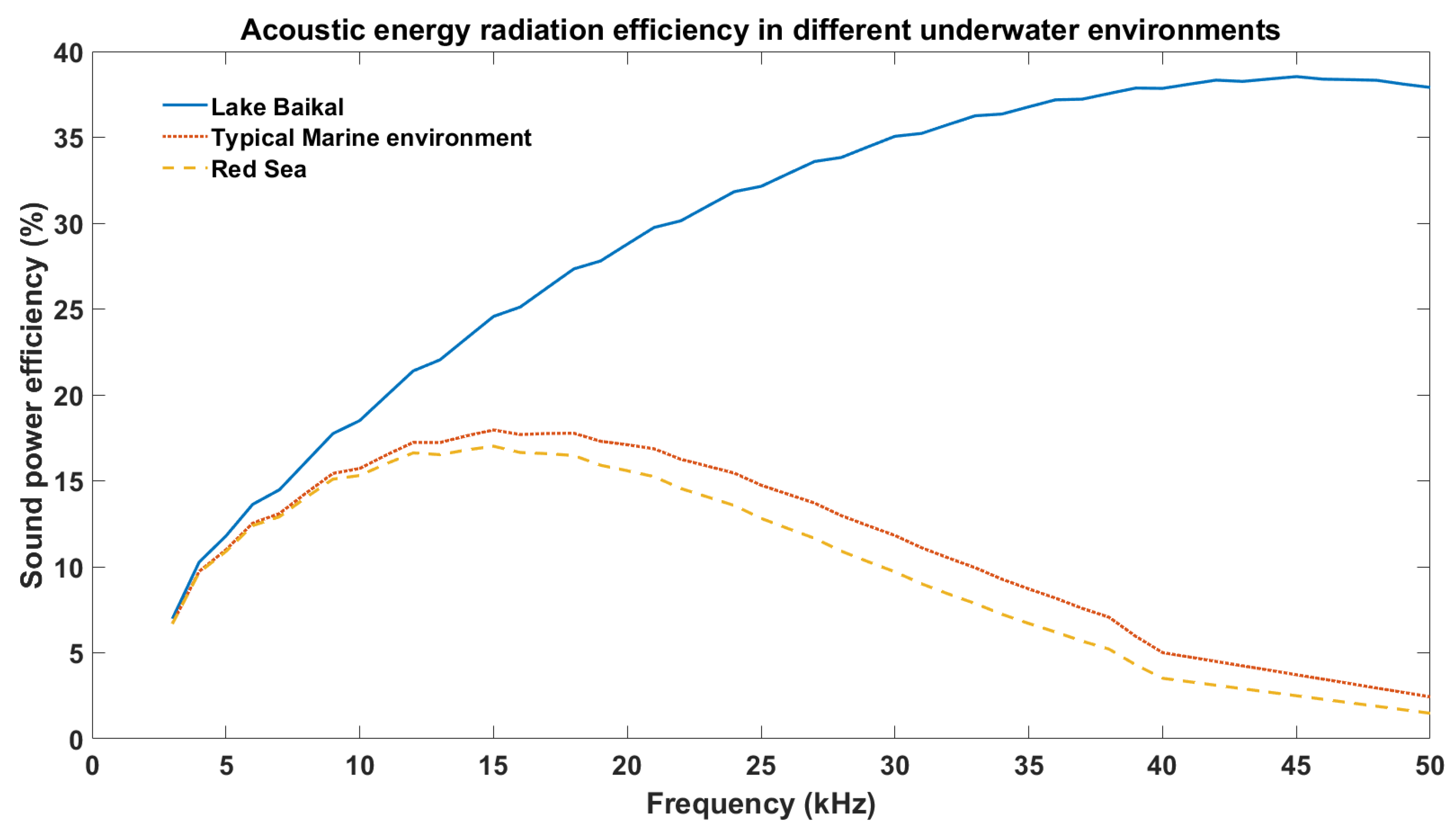
The selected temperatures (0 °C, 20 °C, and 30 °C) used in this study are not arbitrary and deliberately align with three distinct real-world underwater environments that span the spectrum of acoustic absorption characteristics. These temperatures were chosen to rigorously analyze the dynamic balance between absorption and geometric spreading losses under extremes (minimum and maximum absorption attenuation) and typical marine conditions, ensuring the model’s applicability across diverse scenarios:

• 0 °C (Lake Baikal environment):

This temperature represents low-temperature, freshwater environments with minimal absorption attenuation.

Lake Baikal, the world’s deepest freshwater lake, exhibits near-freezing bottom temperatures (~0–4 °C) and negligible salinity (0 PSU).

Such environments yield the lowest absorption coefficients (α) due to the absence of salinity-driven chemical relaxation (e.g., magnesium sulfate contributions) and the reduced viscous losses that occur in cold water.

2.

20 °C (typical marine environment):

This temperature reflects temperate ocean conditions with moderate absorption attenuation.

This temperature is representative of the average surface waters in open oceans (e.g., North Atlantic, Pacific), where the salinity (35 PSU) and temperature jointly govern α through boric acid and magnesium sulfate relaxation mechanisms.

3.

30 °C (Red Sea environment):

This temperature represents high-temperature, hypersaline environments with maximum absorption attenuation.

The Red Sea, characterized by surface temperatures exceeding 30 °C and salinity up to 41 PSU, exhibits peak absorption coefficients due to intensified magnesium sulfate (MgSO₄) relaxation and thermal-enhanced viscous losses.

Boundary conditions: in order to simulate the propagation of sound in open water, boundary conditions are set to avoid the interference of boundary reflections on the simulation results.

Propagation distance and receiving direction: the simulation evaluates the acoustic energy attenuation characteristics at different propagation distances and receiving angles to verify the energy loss mechanism.

3.1.2. Numerical Simulation Design

Numerical modeling of energy loss: numerical computing platform tools are used to numerically model the energy loss, including key variables such as the sound pressure level (SPL), attenuation coefficient, and frequency-dependent absorption loss, in order to quantitatively analyze the impact of acoustic energy loss.

In order to verify the accuracy of the derived theoretical values of the array sound source and to further investigate the equilibrium relationship between geometric diffusion attenuation and absorption attenuation, this study was based on the finite element simulation method and used the MATLAB (Version 9.8 R2020a) numerical computation tool to realize accurate numerical simulation of the radiation characteristics of the sound source in the simulation environment. The core intent of the numerical simulation was to analyze the acoustic transmission efficiency of the simulated array by constructing a specified spherical acoustic domain surrounding the sound source to quantify the contributions of geometric diffusion attenuation and absorption attenuation, and to ultimately to determine the optimal frequency of acoustic energy.

Accurately measuring the three-dimensional distribution of underwater acoustic power requires that a large number of hydrophones be deployed across the entire study domain—or over a closed surface that encloses the sound source. Each hydrophone must record the local sound-pressure amplitude and phase to reconstruct the complete acoustic field. However, in physical experiments, hydrophones cannot be packed densely enough to cover the entire spherical surface without gaps. Physical constraints on sensor size and spacing mean that real arrays will inevitably under-sample certain regions. Moreover, even a dense hydrophone array introduces measurement uncertainties such as calibration errors and electronic noise—and achieving perfect synchronization for phase acquisition is challenging.

Given these limitations, we chose high-fidelity finite-element simulation in place of physical experiments. The simulation conducted herein serves as an ideal experimental setup with extremely high “sensing” density: the entire spherical domain is discretized into small volumetric elements whose dimensions are on the order of the acoustic wavelength. The model computes the pressure field at every point within this three-dimensional grid, offering continuous, high-resolution acoustic field analysis. Because the dense mesh can approximate the sphere with arbitrary precision and provides many more sampling nodes than practical instrumentation, it delivers much higher spatial resolution and, consequently, greater computational accuracy. In other words, the method is immune to sensor noise, coverage gaps, and other instrument-related issues, and can dynamically adjust the spatial resolution according to the frequency of the wavelength, ensuring that no details are lost through under-sampling.

• Construction of an underwater acoustic energy radiation model based on the spatial distribution characteristics of acoustic power.

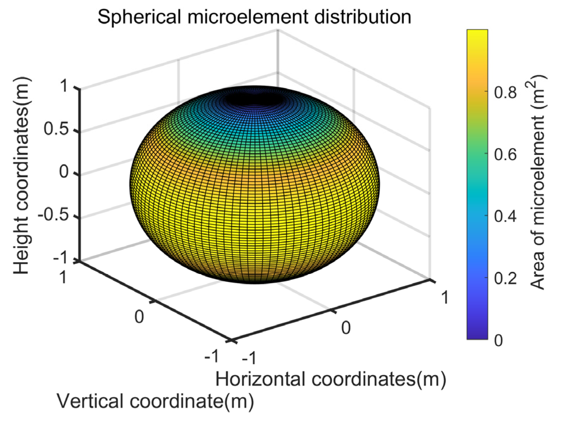
Figure 2 illustrates the discretization strategy that we employed to numerically simulate spherical acoustic domains. This study utilizes the finite element discretization method, subdividing the spherical surface into mesh elements with well-defined element types, sizes, and quantities. To balance simulation accuracy and computational efficiency, based on acoustic wave propagation theory and the Courant–Friedrichs–Lewy stability criterion, this study sets the maximum element edge length to 1/10 of the wavelength corresponding to the highest working frequency, thereby ensuring the accurate capture of acoustic field variations across the entire frequency range during frequency sweeps [47]. Tetrahedral elements are selected to ensure sufficiently fine discretization at the spherical boundary and in regions with large sound pressure gradients. As shown in the figure, the discrete elements exhibit relatively uniform area distribution, which effectively reduces cumulative errors caused by element non-uniformity during numerical integration. Through this meshing strategy, the spatial characteristics of the sound power distribution on the spherical surface can be accurately reflected at different frequencies while stability is ensured in calculating the sound power efficiency.

2.

Quantification of geometric diffusion attenuation

The geometric diffusion attenuation is quantified by calculating the sound power flow on a sound power sphere that surrounds the source. The sound pressure is sampled at discrete points on the sphere and the sound power is obtained by numerical integration over the entire sphere. The area distribution of the microelements in this process directly determines the integration accuracy, so the discretization of the microelements, as shown in Figure 2, is the basis for the reliability of the simulation results.

3.

Calculation of absorption attenuation in aqueous media

The absorption attenuation is analyzed by setting the absorption coefficients of the medium according to measured parameters that are representative of real water conditions, which thereby ensures the fidelity of the simulation results. Specifically, the environmental parameters within the entire acoustic domain—comprising both the sound source and the measurement points—are defined to represent realistic underwater scenarios. By establishing distinct absorption scenarios through variation of these parameters, the effects of absorption attenuation on acoustic power transmission are rigorously assessed and combined with geometric diffusion attenuation. This integrated approach enables a comprehensive and precise quantitative analysis of the acoustic energy loss.

4.

Determination of optimal frequency

The acoustic transmission efficiency at various frequencies is investigated by systematically varying the radiation frequency of the sound source. These simulations focus explicitly on identifying the optimal frequency at which the geometric diffusion attenuation and absorption attenuation achieve equilibrium, which signifies the frequency condition that maximizes the acoustic energy transmission efficiency. The determined optimal frequency provides crucial theoretical guidance for practical acoustic source design.

The acoustic power efficiency value is derived from the sound pressure recorded at the receiver, that is, on the spherical observation surface surrounding the sound source. In other words, our simulation measures the sound pressure field at the receiver and converts it to sound intensity and total acoustic power, which are then used to calculate the transmission efficiency. This pressure → intensity → power → efficiency derivation process inherently accounts for the influence of the received pressure in performance evaluation. This approach is sufficient for assessing energy transmission performance because it condenses the impact of the received pressure into a practical efficiency metric that is relevant to energy transfer evaluation.

3.2. Analysis of Experimental Results on One-Dimensional Linear Arrays

3.2.1. Comparison of Simulation Results with Theoretical Model

Figure 3 illustrates the trend of the acoustic power efficiency with variations in frequency in a one-dimensional linear array model that incorporates the geometric diffusion losses and absorption losses of acoustic energy in water. The data in the figure contain comparisons between the simulation and the theoretical model for different propagation distances (100 m and 1000 m) and reception angles (10° and 20°). A detailed analysis of the results is presented below.

Error analysis: As shown in

Table 3. Error analysis of simulation value and theoretical value.

Distance\Angle	100 m\20°	1000 m\20°	100 m\10°	1000 m\10°
Relative Error	0.24%	0.0938%	0.51%	0.29%
Mean Squared Error	$1.643\times {10}^{-6}$	$1.1885\times {10}^{-7}$	$6.3390\times {10}^{-6}$	$7.5555\times {10}^{-7}$

, a detailed error analysis is performed in this paper to quantify the difference between the theoretical values and the simulation results. The small deviations that can be observed are attributed to boundary effects, i.e., the acoustic wave propagation region is discretized into a finite number of grid cells in the numerical simulation. The discretization at the boundary may lead to the accumulation of numerical errors, especially in the case of high frequencies or high accuracy requirements, and the computational errors near the boundary may be more significant. However, these differences are within acceptable limits and are sufficient to support practical applications. The energy loss values at different frequencies are compared with the theoretical values, and the results show a high degree of agreement, verifying the accuracy of the simulation results.

Frequency dependence of the loss mechanism: the analysis confirms that the energy loss in the simulation follows the expected frequency-dependent trend, with higher frequencies exhibiting higher absorption losses. This is consistent with our theoretical predictions and further validates the reliability of the numerical simulation experiments.

3.2.2. Frequency Optimization Analysis Combining Absorption and Diffusion Losses

Figure 3 gives the results of the acoustic power energy transfer efficiency for different frequencies after combining geometric diffusion attenuation and absorption attenuation. The acoustic energy transfer efficiency increases rapidly with an increasing frequency in the low-frequency band (from 0 to 50 kHz) and peaks between 50 and 100 kHz. At this time, the directivity of the array is increased so that the acoustic energy is more concentrated, and the geometrical diffusion and absorption losses are relatively low; thus, the acoustic energy can be radiated efficiently.

In the high-frequency band (>100 kHz), the acoustic power efficiency gradually decreases. In particular, the decrease in efficiency is more significant at a propagation distance of 1000 m. This is because the absorption loss of high-frequency acoustic waves propagating through water increases significantly compared to low-frequency waves, resulting in a rapid decay of the energy and thus limiting the effectiveness of high-frequency acoustic waves in long-distance propagation.

Overall, the acoustic power efficiency is small at lower frequencies, gradually increases with increasing frequency, and begins to decrease after reaching a maximum value in a certain frequency band. This suggests that there is an optimal operating frequency in underwater acoustic wave propagation that maximizes the energy transfer efficiency.

Determination of the optimal frequency: At short distances (100 m), geometric diffusion losses are the main energy loss factor, so higher frequencies help to enhance the directivity of the array and reduce geometric diffusion losses, which in turn improves the sound power efficiency. In the higher frequency range (from 50 to 72 kHz), the energy distribution of the sound waves is more concentrated, resulting in optimal efficiency.

In long-distance (1000 m) propagation, the acoustic absorption loss becomes a dominant factor, especially in the high-frequency band (>50 kHz). Therefore, low frequencies need to be preferred in this case to minimize the effect of absorption losses. The optimal frequencies shown in

Table 4. The optimal frequency of one-dimensional linear array in different propagation distances and receiving directions (the value in brackets is the sound energy radiation efficiency at the optimal frequency).

Distance\Angle	100 m\20°	1000 m\20°	100 m\10°	1000 m\10°
Theoretical Result	54 kHz (47.89%)	24 kHz (44.58%)	69 kHz (46.80%)	36 kHz (42.52%)
Simulation Result	54 kHz (47.85%)	24 kHz (44.60%)	72 kHz (46.88%)	36 kHz (42.40%)

are in the low-frequency band (from 24 to 36 kHz), which makes it easier to balance the geometric diffusion and absorption losses and to maximize the energy transfer efficiency.

Optimal array configuration:

Table 5. The number of array elements needed to achieve optimal energy transmission efficiency.

Distance\Angle	100 m\20°	1000 m\20°	100 m\10°	1000 m\10°
Theoretical Result	55	25	70	37
Simulation Result	55	25	73	37

shows the number of array elements required for optimal energy transfer efficiency at different propagation distances and reception angles. As can be seen from the table, the number of array elements that are required varies with the reception angle and propagation distance, reflecting the trade-off between geometric diffusion loss and acoustic absorption loss under different conditions.

Since the array length is fixed at 0.75 m, an increase in the number of array elements will have a direct impact on the design cost. For short-distance and high-precision applications, it is recommended to design arrays with a higher number of array elements to ensure the best energy transmission efficiency under high-frequency conditions. For long-distance and low-frequency applications, it is recommended that a small number of arrays be designed to meet the needs of directivity and transmission efficiency while reducing the complexity and cost of the equipment.

Through systematic simulation and theoretical analysis, this study reveals the equilibrium relationship between geometric diffusion loss and absorption attenuation at different frequencies, which provides a scientific basis for the frequency optimization of underwater acoustic energy transmission. In practical applications, the findings of this paper can guide the design of acoustic source and receiver arrays, especially in the development of efficient acoustic energy transmission systems.

3.2.3. Comparison of Experimental Results with Different Array Sizes

Figure 4 shows the acoustic energy transmission efficiencies of one-dimensional linear arrays with lengths of 0.75 m and 0.5 m at different propagation distances (100 m and 1000 m) and different receiving directions (10° and 20°).

High-frequency range (>150 kHz): The sound power efficiencies of arrays of different sizes decrease rapidly with an increasing frequency, and the decrease is more pronounced at larger propagation distances (1000 m). This further confirms that high-frequency sound waves are mainly limited by absorption attenuation when traveling over long distances. A longer array length (0.75 m) has a slightly higher efficiency in the high-frequency band, suggesting that the array size plays a role in the directivity enhancement of high-frequency sound waves.

Mid-frequency range (50–150 kHz): The sound power efficiency peaks in this frequency range with an efficiency of about 40%. Frequencies in this range correspond to the equilibrium between geometric diffusion attenuation and absorption attenuation. An array length of 0.75 m is slightly more efficient than 0.5 m, indicating that larger arrays focus the acoustic energy better in the mid-frequency range.

Low-frequency range (<50 kHz): The sound power efficiency decreases rapidly in the low-frequency range, mainly due to the longer wavelengths of the low-frequency sound waves, which significantly reduce the directivity and radiation efficiency of the array.

The values in

Table 6. The optimal frequency and number of array elements for achieving the optimal acoustic radiation energy efficiency at different propagation distances and receiving directions (the length of the array is 0.5 m).

Distance\Angle	100 m\20°	1000 m\20°	100 m\10°	1000 m\10°
Optimal Frequency	63 kHz	27 kHz	60 kHz	27 kHz
Sound energy radiation efficiency	47.24%	43.54%	46.04%	41.47%
Number of array elements	43	19	41	19

(optimal frequencies for the 0.5 m linear array at various distances/angles) were identified by analyzing where the simulation’s efficiency curve reached its maximum under each condition. This was done after ensuring that the frequency sampling was fine enough (1 kHz) to obtain a reasonable level of accuracy.

The shorter arrays (e.g., 0.5 m) exhibited a slight optimal frequency shift compared to the longer arrays (e.g., 0.75 m), emphasizing the effect of array layout parameters on the geometric diffusion losses. These results are further quantified in Table 5 and Table 6. Interestingly, smaller arrays only require fewer array elements to achieve optimal performance. However, this is also accompanied by a decrease in the radiation efficiency, especially in the lower-frequency bands. This suggests that there is a balance to be struck between efficiency and cost and also suggests that smaller arrays may be preferred in cost-sensitive designs, with larger arrays being preferred in efficient designs.

3.3. Performance Comparison and Analysis of Two-Dimensional Planar Arrays

Although one-dimensional linear arrays show some advantages in directionality and pointing control, their ability in spatial coverage and multi-dimensional pointing is still limited, especially in complex underwater environments or application scenarios that require larger coverage angles.

In attempting to further enhance the spatial coverage capability of acoustic energy transmission and to better adapt to multi-angle and multi-distance applications, two-dimensional array structures become a natural extension and optimization option. Compared to one-dimensional arrays, two-dimensional arrays are not only capable of controlling the acoustic radiation in both the horizontal and vertical directions in a balanced manner, but are also capable of obtaining more precise beam control due to the ease of adjusting the layout of the array elements. Therefore, in the following analysis, we will explore the performance of two-dimensional arrays under various propagation distances, reception angles, and operating frequencies. The term “operating frequencies” here refers specifically to the discrete frequency values that were systematically selected from within the frequency sweep range, as detailed previously in the experimental setup. This analysis will focus on evaluating the advantages and challenges associated with two-dimensional arrays in terms of their acoustic energy radiation efficiency, directivity control, and overall system cost under these varying conditions.

In the previous analysis, by comparing the acoustic energy radiation efficiencies of one-dimensional linear arrays at different propagation distances, reception angles, and frequencies, it was found that the simulation results were highly consistent with the theoretical values. This consistency verifies the reliability of the simulation model and shows that, under the current parameter settings and computational methods, the simulation can effectively reflect the expected results of the theoretical model, especially in terms of the energy transfer efficiency and the number of array elements required at different frequencies and array configurations.

Given that the simulation results of the one-dimensional array are in high agreement with the theoretical results, they provide a reliable basis for the subsequent analysis. Therefore, in the next two-dimensional array analysis, we will mainly use the simulation results in order to evaluate the acoustic energy radiation efficiency of the two-dimensional array under different propagation distances and reception angles. By analyzing the performance of the 2D array through simulation, we can more effectively study its directivity control and spatial coverage capability, as well as balancing its capabilities with the design cost, in complex application scenarios, so as to provide more detailed data support for the optimization of the 2D array in practical applications.

In this study, we synthesize different structures of 2D arrays, including equally spaced hexagonal arrays and circular arrays. Figure 5 illustrates two array configurations, and Figure 6 presents the frequency-dependent curves of acoustic power radiation efficiency for these two arrays after accounting for both geometric spreading loss and underwater acoustic absorption loss.

Table 7. Parameter configuration of hexagonal array for optimal acoustic radiation efficiency.

Distance\Angle	100 m\20°	1000 m\20°	100 m\10°	1000 m\10°
Optimal Frequency	37 kHz	19 kHz	52 kHz	28 kHz
Sound energy radiation efficiency	49.29%	47.00%	49.05%	46.16%
Array layer number	14	8	19	11
Number of array elements	547	169	1027	331

and

Table 8. Parameter configuration of circular array for optimal acoustic radiation efficiency.

Distance\Angle	100 m\20°	1000 m\20°	100 m\10°	1000 m\10°
Optimal Frequency	34 kHz	16 kHz	49 kHz	25 kHz
Sound energy radiation efficiency	49.38%	47.28%	49.23%	46.54%
Array layer number	13	7	18	10
Number of array elements	497	136	970	288

give the optimal frequency, corresponding number of array layers, and number of array elements required for the circular array to achieve the optimal underwater energy transfer efficiency. Figure 6 further compares the sound pressure level distributions of the acoustic fields of the circular and hexagonal arrays under the same conditions, aiming to evaluate the performance of different array structures in underwater acoustic radiation.

3.3.1. Frequency Dependence of Sound Power Radiation Efficiency

In both two-dimensional, equally spaced arrays, the hexagonal array and the circular array, the trend of the acoustic power radiation efficiency with the frequency shows some regularity. In the low-frequency band, the radiation efficiency rises rapidly with an increasing frequency and then peaks in the mid-frequency band. This is due to the significantly increased directivity of the array in this frequency range, for which the geometric diffusion loss is smaller and the effect of absorption loss is not yet significant. In the high-frequency band, the radiation efficiency decreases rapidly, especially in long-distance propagation (e.g., 1000 m), and this decrease is mainly influenced by the cumulative effect of absorption losses in the water.

Although both arrays exhibit similar frequency response trends, their optimal frequency ranges are slightly different. As shown in Table 7 and Table 8, the optimum frequency range of the hexagonal array is 19–52 kHz, while the optimum frequency range of the circular array is 16–49 kHz. This variation indicates that the geometric configurations of the arrays significantly influence their frequency response characteristics, affecting the optimal operational frequency ranges and the acoustic radiation efficiency that is achievable by each array design.

3.3.2. Effect of Array Structure on Energy Transmission Performance

The two arrays also differ in the number of array layers and the number of array elements that are required to achieve optimal performance. In short-range, high-frequency (HF, defined here as frequencies above approximately 20 kHz) applications, the hexagonal array (10° reception angle, 100 m) requires 19 layers and 1027 array elements, while the circular array requires 18 layers and 970 array elements under similar conditions. The structural complexity of both arrays decreases in long-range, low-frequency scenarios, e.g., at 1000 m and a 20° reception angle: the hexagonal array requires only eight layers and 169 array elements, while the circular array requires seven layers and 136 array elements.

3.3.3. Interaction of Geometric Diffusion Losses with Absorption Losses

The geometric diffusion loss and absorption loss, together, determine the pattern of change in the efficiency of sound power radiation. In short-distance propagation (e.g., 100 m), geometric diffusion loss is the dominant factor, so the directivity and energy concentration of the array can be significantly enhanced by increasing the frequency. In long-distance propagation (e.g., 1000 m), the absorption loss gradually dominates, and the energy attenuation under high-frequency conditions is significant. The optimal frequencies of both arrays show a decreasing trend with an increasing propagation distance, indicating that lower frequencies need to be selected to reduce absorption losses in long-distance propagation.

3.3.4. Sound Field Distribution Analysis

Figure 7 shows the sound field and sound pressure level distribution of the hexagonal array and the circular array at a frequency of 28 kHz. From the distributions of the sound field and sound pressure level, it can be seen that the sound field of the hexagonal array has a more complex sidelobe structure and more uniform spatial coverage characteristics. This “striped” distribution is suitable for application scenarios that require wide coverage and multi-target monitoring. In contrast, the sound field distribution of the circular array is more regular, with fewer side lobes and a higher main lobe concentration, and the energy is radiated in an almost symmetrical circular manner. This feature makes the circular array suitable for applications that require high directivity and concentrated sound energy transmission.

3.4. Analysis of Numerical Simulation Results of Different Underwater Environments

3.4.1. Effects of Various Ocean Environmental Parameters on Underwater Acoustic Energy Transmission

In this study, two extreme real underwater environments and an average typical marine environment were experimentally analyzed to investigate the equilibrium relationship between geometric diffusion loss and absorption attenuation during acoustic propagation and to explore the possibility of optimizing the transfer of acoustic energy under different frequency conditions.

As shown in Figure 8, the three underwater environments represent are as follows [48]:

Low absorption attenuation coefficient (LACO) environments: Deep, cryogenic freshwater environments characterized by low salinity (approximately 0 PSU), low temperatures (near freezing), and high pressures with extremely low absorption attenuation coefficients. A qualifying real-world environment is Lake Baikal, which has a maximum depth of more than 1600 m and a bottom water temperature of nearly 4 °C [49].

High absorption attenuation coefficient environment: A high-salt, high-temperature marine environment characterized by high salinity (41 PSU), high temperatures (approximately 30 °C or more in the surface layer), and a high absorption attenuation coefficient [50]. The Red Sea is surrounded by the Arabian Peninsula and the African continent, with limited exchange with the outer sea, high evaporation rates, scarce precipitation, and no significant freshwater river inflow. This closed geographical structure further contributes to the uniqueness of the Red Sea’s salinity and temperature [51]. These characteristics make the Red Sea one of the real sea areas with the highest absorption attenuation.

Typical average marine environment: Represents a typical average marine environment (conventional salinity 35 PSU, temperature 20 °C, depth 0 m, absolute pressure $\approx 1 \mathrm{atm}$).

By comparing the geometric diffusion loss and absorption attenuation effects in these three environments, the combined effect of the two is investigated at different frequencies and the optimal frequency for acoustic energy transfer is determined.

The horizontal axis of Figure 9 is the frequency (unit: kHz), and the vertical axis is the acoustic energy radiation efficiency (unit: %). Using a circular array with a radius of 0.25 m, under the conditions that the propagation distance is 1000 m and the reception direction is 5°, the change rule of the acoustic energy radiation efficiency with the frequency is studied in three typical environments.

Lake Baikal environment: the highest acoustic energy radiation efficiency is found in the 10–50 kHz range, with a peak efficiency close to 35%.

Typical marine environment: the acoustic energy radiation efficiency peaks at about 25% in the low- and middle-frequency bands (10–30 kHz) but decreases more rapidly in the higher frequency bands.

Red Sea environment: the overall efficiency is the lowest, especially in the frequency range above 20 kHz, where the efficiency decreases rapidly. The high-salinity and high-temperature conditions of the Red Sea greatly increase the absorption attenuation effect, leading to severe energy loss in the high-frequency band.

By comprehensively analyzing the acoustic absorption attenuation coefficients and acoustic energy radiation efficiencies of the Lake Baikal, typical marine, and Red Sea environments, the optimal operating frequency ranges and applicable conditions for each environment can be clarified. This provides important theoretical support for the design and optimization of acoustic equipment for different underwater environments.

3.4.2. Environmental Adaptability Design for Optimized Sound Energy Propagation

Through the analysis of the three typical environments, the following conclusions and design recommendations can be drawn.

Frequency selection and environmental adaptation: In low-absorption environments (such as Lake Baikal), medium- and low-frequency designs should be preferred due to their low absorption characteristics. In high-absorption environments (such as the Red Sea), it is recommended to use low-frequency solutions to reduce absorption losses while optimizing the directivity design of the equipment sound field and concentrating the sound energy through the optimization of the array structure (such as increasing the array density) to cope with high-frequency energy losses and reduce the impact of geometric diffusion. In typical marine environments, the frequency should be dynamically adjusted according to the propagation distance and receiving direction, as discussed previously, to balance the absorption and geometric diffusion.

4. Conclusions

In this study, the balance between geometric diffusion and absorption attenuation in hydroacoustic energy transmission is systematically investigated, and an optimized frequency selection framework is proposed to improve the transmission efficiency in complex underwater environments. The research results show the following.

Geometric diffusion and absorption attenuation equilibrium: This paper proposes the equilibrium theory of absorption attenuation and diffusion attenuation and clarifies their dynamic relationship by quantitatively analyzing the interaction mechanism between them. The interaction between geometric diffusion and absorption attenuation is frequency-dependent. At shorter propagation distances, geometric diffusion dominates the energy loss, while at longer distances, absorption attenuation becomes dominant. This equilibrium relationship significantly affects the optimal frequency selection for hydroacoustic energy transfer systems.

Optimum frequency identification: A quantitative method was developed to determine the optimum frequency to achieve maximum transmission efficiency. The results identify a range of peak efficiencies, typically located between low and middle frequencies (20–100 kHz), depending on the sound propagation distance and the configuration of the source array parameters. The optimal frequency determined in this paper ensures that the energy loss from the combination of the two energy attenuation mechanisms is minimized.

Influence of environmental parameters: Changes in underwater environmental variables such as the salinity, temperature, and depth can affect the absorption characteristics of the environment. By comprehensively analyzing the acoustic absorption attenuation coefficient and acoustic energy radiation efficiency under actual underwater environmental parameter settings, the optimal operating frequency range and applicable conditions for each environment can be clarified. This provides important theoretical support for the design and optimization of acoustic equipment for different underwater environments.

Engineering design guidance: The proposed frequency optimization strategy provides actionable engineering guidance for hydroacoustic array design. The results of this study allow dynamic frequency tuning to specific operating environments and application requirements. In addition, array configurations should be adapted to balance geometric diffusion and absorption losses, and the design trade-offs between efficiency and cost should be considered.

Overall, this study bridges the gap between the theoretical and practical analysis of hydroacoustic energy transfer by providing a robust analytical framework and practical guidelines for array and frequency optimization. These contributions not only extend the depth of theoretical analysis, but also have great potential for application in underwater communication, resource exploration, and acoustic monitoring systems.

Future work will explore the impact of real-world applications and non-ideal conditions (e.g., turbulence and biological noise) on the proposed equilibrium relationship optimization model. In addition, we acknowledge the potential value of impulse excitation to specific applications (e.g., short-range sonar or transient signal analysis). In future studies, we plan to extend the framework to include time-domain simulations for scenarios that require transient analysis and to validate pressure waveforms experimentally using calibrated hydrophones in controlled underwater environments. While this study focuses on theoretical and numerical rigor, we fully acknowledge the value of experimental validation. Future work will collaborate with ocean engineering teams to deploy prototype systems in real marine environments.