Abstract
This study presents a comparative numerical investigation of Reynolds-averaged Navier–Stokes (RANS) and partially averaged Navier–Stokes (PANS) turbulence models applied to the Joubert BB2 submarine geometry under steady, calm-water conditions. To assess the influence of turbulence resolution and grid density on hydrodynamic performance prediction, simulations were conducted using three mesh resolutions—coarse, medium, and fine—based on unstructured hexahedral grids. The results were validated against international benchmark data, with emphasis placed on total resistance, pressure and shear stress distributions, wake development, and vortex structure. The PANS model consistently outperformed RANS in accurately predicting total resistance and resolving wake asymmetry, especially at medium grid resolution, due to its ability to partially resolve turbulence without full reliance on eddy viscosity assumptions. It demonstrated superior capability in capturing coherent vortex structures and preserving axial momentum in the stern region, resulting in more realistic surface pressure recovery and delayed boundary layer separation. Cross-sectional and circumferential velocity distributions in the propeller plane further highlighted PANS’s enhanced turbulence fidelity, which is essential for downstream propeller performance evaluation. Overall, the findings support the suitability of the PANS model as a practical and computationally efficient alternative to RANS for high-fidelity submarine flow simulations, particularly in wake-sensitive applications where LES remains computationally prohibitive.
1. Introduction
The accurate prediction of hydrodynamic forces and wake behavior around submerged bodies remains a cornerstone challenge in naval hydrodynamics, particularly for streamlined geometries such as submarines. Among benchmark configurations, the Joubert BB2 submarine has become widely accepted in the research community due to its publicly available geometry and accompanying international validation data. In addition to its widespread use in CFD validation, the BB2 submarine has also been the subject of recent experimental investigations. For example, Kim et al. [1,2] conducted planar motion mechanism (PMM) tests and hydrodynamic measurements on the BB2 model, evaluating the effects of control plane deflection and hull motion states on force coefficients. These recent studies provide valuable experimental datasets that serve as benchmarks for validating numerical predictions, and they highlight the importance of integrating physical measurements with turbulence modeling assessments. As an ideal platform for assessing computational fluid dynamics (CFD) methods, the BB2 configuration enables systematic studies of resistance characteristics, wake structures, and turbulence modeling performance.
In the past two decades, Reynolds-averaged Navier–Stokes (RANS) models have been the workhorse of industrial CFD due to their robustness and relatively low computational cost. Numerous studies have utilized RANS to simulate resistance and wake flow features of underwater vehicles, demonstrating reasonable agreement with experiments when appropriately calibrated. For instance, Chen et al. [3] conducted numerical simulations of the BB2 submarine during near-surface turning maneuvers, capturing variations in resistance and propeller loading as a function of submergence depth. Their results highlighted the importance of accounting for dynamic free-surface effects and attitude changes when simulating operational conditions. In a separate study, Dogrul [4] investigated the scale effects on the propulsion performance of the BB2 submarine using the body force method in conjunction with RANS simulations. This work provided valuable insights into the discrepancy between model- and full-scale performance metrics, such as wake fraction and propulsive efficiency, demonstrating the role of turbulence modeling in extrapolating experimental data. Additionally, the influence of strut installations on BB2 hydrodynamics was examined by Park and Seok [5], who quantified the distortion of the local inflow field and the amplification of pressure resistance across multiple drift angles. Their findings emphasized the need to consider support-induced perturbations in both physical experiments and CFD validations.
Beyond resistance and propulsion, wake characteristics and associated acoustic emissions have also been a major focus in BB2-related CFD research. Wall-modeled large eddy simulation (WMLES) was applied by Rocca et al. [6] to analyze the hydroacoustic behavior of the BB2 geometry. By solving the Ffowcs Williams–Hawkings equation, the study demonstrated that fine-scale turbulence resolution is crucial for capturing pressure fluctuations near the propeller plane that contribute to noise generation. Similarly, advanced turbulence modeling techniques such as LES have been used to resolve complex wake structures around submarines. For example, Chen et al. [7] performed LES of the BB2 under straight-ahead and yaw conditions, capturing anisotropic vortex development and asymmetric pressure distributions that are typically underrepresented in RANS solutions. Furthermore, turbulence model selection has been shown to significantly influence the quality of wake predictions in bluff-body flows. Huong et al. [8] compared several turbulence models in predicting the downstream wake features of a Rood wing, revealing model-dependent discrepancies in velocity deficit, vortex coherence, and turbulent kinetic energy decay. These results collectively demonstrate the limitations of conventional RANS models, particularly in flows dominated by unsteady, anisotropic turbulence and complex wake development.
Although LES offers high-fidelity predictions by explicitly resolving large-scale turbulent structures, its practical application in ship hydrodynamics remains challenging due to the stringent grid and time-step requirements. As discussed by Liefvendahl and Fureby [9], wall-resolved LES (WRLES) demands prohibitively high computational costs, especially at high Reynolds numbers, due to the need to resolve viscous sublayers within turbulent boundary layers over the entire hull surface. Even WMLES, though more efficient, still requires millions to billions of grid cells for full-scale simulations. Furthermore, the reliability of LES is sensitive to factors such as numerical dissipation, subgrid-scale (SGS) model choice, and mesh irregularities, particularly when using unstructured grids in complex configurations, as demonstrated by Ouvrard et al. [10] in simulations of bluff-body flows.
To overcome these limitations, hybrid turbulence modeling approaches have been actively developed, offering an intermediate solution between the cost-effectiveness of RANS and the high fidelity of LES. Detached eddy simulation (DES) is one of the earliest hybrid models and was designed to switch from RANS to LES in regions of high flow unsteadiness. For example, Nisham et al. [11] applied DES to predict the airwake behavior around a full-scale naval ship in head waves, demonstrating its capability to capture unsteady airwake dynamics under varying wave and wind conditions. While DES improved the prediction of large-scale flow features over conventional RANS, it suffered from premature switching to LES mode in near-wall regions, potentially compromising near-surface accuracy.
To mitigate this, the delayed detached eddy simulation (DDES) was introduced by redefining the length scale to prevent early LES activation in boundary layers. Ren et al. [12] employed DDES in simulating planar motion mechanism (PMM) tests of a ship hull and found that DDES significantly improved the representation of vortex structures and turbulent kinetic energy distribution compared to RANS. Notably, DDES captured more realistic shear-layer development and wake turbulence, which are critical for understanding hull maneuvering behaviors.
More recently, the improved delayed detached eddy simulation (IDDES) model was developed to further enhance hybrid RANS/LES performance in wake prediction by refining transition criteria and eddy viscosity formulation. Zhang et al. [13] applied IDDES to investigate the wake flow behind a generic ship model and showed that while global drag predictions remained largely insensitive to numerical settings, local wake structures were highly dependent on grid resolution and discretization schemes. Their findings underscored the importance of resolving wake asymmetry and vortex shedding for accurate wake analysis goals that standard RANS often fails to achieve.
Despite the growing sophistication of hybrid models, their performance still varies significantly with grid quality and case-specific flow conditions. As an alternative, the partially averaged Navier–Stokes (PANS) model, originally proposed by Girimaji [14], provides a bridging approach between RANS and DNS without requiring explicit zonal decomposition. Unlike DES-type models, PANS allows for continuous variation in turbulence resolution depending on the grid and model control parameters (e.g., , ) enabling better adaptability to local flow features. Recent studies have validated its capability in complex marine and bluff-body flows. Zhang et al. [15] applied PANS to the flow past a generic ship and found that it produced wake structures and coherent vortex-shedding patterns similar to LES at a fraction of the computational cost. Bensow and Boogaard [16] evaluated PANS for the Japan Bulk Carrier (JBC) and reported that medium-scale turbulence features could be captured even with moderate grid density, making PANS promising for industrial ship applications. Moreover, the PANS model has been extended to propeller and cavitation simulations. For instance, Ji et al. [17] integrated PANS with a modified model to simulate cavitating flow around a marine propeller in a non-uniform wake, successfully capturing unsteady cavitation patterns that conventional RANS models failed to reproduce. Similarly, Kamble and Girimaji [18] demonstrated that PANS provides improved predictions of turbulent wake anisotropy and coherent structures around spheres and bluff bodies. These studies collectively demonstrate that PANS achieves a balance between fidelity and computational feasibility and is particularly well suited for simulations involving wake evolution, vortex dynamics, and transient resistance. Despite these promising results, applications of PANS in fully wetted submarine flows such as the Joubert BB2 remain limited. In particular, there is a lack of systematic grid sensitivity studies comparing PANS and RANS under identical boundary conditions and geometries. Therefore, the present study aims to fill this gap by performing a comparative CFD investigation of RANS and PANS turbulence models applied to the BB2 submarine configuration.
Therefore, the present study aims to conduct a comprehensive CFD investigation of the Joubert BB2 submarine using both RANS and PANS turbulence models. Special emphasis is placed on evaluating resistance components, wall shear and pressure distributions, wake structures, and grid sensitivity to understand how turbulence resolution influences flow physics and numerical accuracy. Validation is achieved through comparison with internationally recognized RANS datasets, ensuring consistency and reliability. This paper is structured as follows. Section 2 outlines the numerical methodology, including geometry setup, turbulence modeling, and grid strategy. Section 3 presents and compares the simulation results in terms of resistance components, flow fields, and wake characteristics. Finally, Section 4 concludes the paper by summarizing the key findings and suggesting directions for future research.
2. Numerical Methodology
2.1. Governing Equations
This study employs two turbulence modeling approaches for incompressible, unsteady flow: Reynolds-averaged Navier–Stokes (RANS) and partially averaged Navier–Stokes (PANS). Both methods are formulated using the filtered form of the Navier–Stokes equations, with the Shear Stress Transport (SST) model [19,20,21] used as the baseline turbulence closure. The primary difference lies in how the turbulent scales are treated: RANS models the entire turbulence field, while PANS resolves a portion of the turbulence spectrum based on grid resolution and user-defined parameters [14,22].
2.1.1. Reynolds-Averaged Navier–Stokes—(RANS)
The RANS model governs the mean behavior of turbulent flows by averaging the instantaneous equations over time. Based on the formulation described by Alfonsi [23], the resulting equations for mass and momentum conservation in an incompressible Newtonian fluid are given as follows:
where and denote the time-averaged velocity and pressure, respectively, and is the Reynolds stress tensor representing the effect of unresolved turbulence. To close the equations, the Boussinesq eddy viscosity hypothesis is applied:
The eddy viscosity is evaluated using the SST model [19,20,21], which blends the standard model near walls with the model in the outer flow. The transport equations for the turbulent kinetic energy and specific dissipation rate were expressed in Equations (5) and (6). In particular, the equation for includes the cross-diffusion term, in which the blending function () is applied to represent the gradual transition between the and models. This treatment follows the SST formulation and is essential for improving numerical stability and model accuracy in near-wall and free-shear regions. Readers are referred to Pereira et al. [24] for further details on the derivation and implementation of this term.
The eddy viscosity is calculated as follows:
where is a blending function ensuring a smooth transition between and behavior. The constants , , , , and are determined based on Menter’s SST formulation [19,20,21].
2.1.2. Partially Averaged Navier–Stokes—(PANS)
The PANS model, introduced by Girimaji [14], is a variable-resolution turbulence modeling approach that allows a seamless transition between RANS and DNS by selectively resolving turbulent scales. It is derived from filtering the Navier–Stokes equations over a portion of the turbulence spectrum.
The filtered continuity and momentum equations, as proposed by Girimaji [14], are given by the following:
where and denote the partially averaged velocity and pressure, and represents the sub-filter scale (SFS) stress tensor. Using a Boussinesq-like approach, we obtain the following:
Here, and are the unresolved turbulent kinetic energy and dissipation rate, respectively, and is the resolved strain-rate tensor. The governing transport equations for these unresolved quantities are presented in Equations (12) and (13), based on the PANS formulation of the SST model. In Equation (13), the cross-diffusion term was introduced to maintain consistency with the SST-based formulation. This term includes the blending function (), which ensures a smooth model transition and enhances accuracy in partially resolved turbulence regions. The detailed formulation and rationale can be found in Pereira et al. [24]. These equations incorporated several model constants—such as and —that controlled the production, dissipation, and diffusion terms within the PANS formulation. The functional forms of these constants followed those reported by Seok et al. [25].
To control the degree of resolution, PANS introduces two resolution control parameters introduced by Lakshmipathy and Girimaji [22]:
These parameters define the modeled portion of the turbulence spectrum. When , the PANS model reduces to a RANS solution while approaches DNS-like resolution. In this study, the dynamic PANS method is adopted, where is locally adjusted based on grid scale and turbulence length scale, which was proposed by Luo et al. [26]:
where is the characteristic local cell size.
2.2. Numerical Methods
In this study, all simulations were conducted using a finite volume framework implemented in OpenFOAM version 7. The governing equations were discretized using second-order accurate schemes in both space and time to ensure numerical consistency and minimize discretization error in the unsteady turbulent flow field. For temporal discretization, the Crank–Nicolson scheme was employed, providing second-order accuracy and improved stability for transient simulations. A time-weighting coefficient of 0.9 was applied to introduce a slight implicit damping effect, which helps suppress numerical oscillations in stiff regions without compromising accuracy. Spatial discretization of the divergence terms (notably the convective fluxes) and gradient terms was performed using the Gauss linear scheme with central differencing. This second-order accurate approach provides a balance between accuracy and computational efficiency in resolving boundary layers and wake structures, which is especially important in turbulence-resolving simulations such as those based on the PANS model.
To maintain pressure–velocity coupling, the PIMPLE algorithm was used. This algorithm combines the advantages of both SIMPLE (Semi-Implicit Method for Pressure-Linked Equations) and PISO (Pressure Implicit with Splitting of Operators) algorithms. Specifically, PIMPLE enables efficient handling of transient flows with moderate Courant numbers while maintaining iterative pressure correction within each time step. In this study, a maximum of 3 outer correctors and 2 inner correctors were employed per time step, which was found sufficient to ensure convergence without excessive computational cost. Non-orthogonal and skewness corrections were also activated to accommodate local mesh irregularities, particularly near the stern and appendages where complex geometry-induced distortions may arise. A bounded linear upwind scheme was applied to the turbulent transport equations to enhance stability in regions with high-velocity gradients while preserving second-order accuracy.
The Courant–Friedrichs–Lewy (CFL) number was maintained below 0.5 in all simulations to ensure temporal stability and allow for accurate resolution of unsteady flow features. Residual convergence criteria were set to for velocity and pressure, and for turbulence quantities, ensuring high-fidelity convergence within each time step.
3. Computational Setup
3.1. Geometry of Target Submarine
The target geometry used in this study is the generic submarine Joubert BB2, a benchmark configuration widely employed in the hydrodynamic research community to validate computational and experimental methodologies. The full-scale length of the BB2 submarine is 70.2 m, and its design includes a cylindrical hull with an X-type stern rudder configuration, a sail, and bow planes. The principal particulars of the Joubert BB2 are summarized in Table 1. For CFD analysis, the model-scale geometry, scaled down by a factor of 18.348, was adopted to ensure consistency with model test conditions. The three-dimensional representation of the model-scale geometry is illustrated in Figure 1. The X-rudder system features high control authority and independent actuation of each stern fin, offering superior maneuverability. To facilitate resistance prediction under calm-water conditions, the rudders and control surfaces were maintained in a neutral position throughout the simulations.

Table 1.
Main particulars of Joubert BB2.
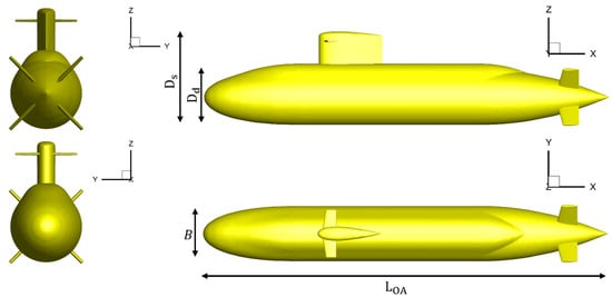
Figure 1.
Three−dimensional view and principal dimensions of the Joubert BB2 submarine geometry used in the present study.
3.2. Computational Domain and Boundary Conditions
The computational domain used in this study is illustrated in Figure 2. The domain was configured to minimize any artificial blockage effects while ensuring the proper development of flow around the model. The domain extends upstream from the bow to the inlet boundary and downstream from the stern to the outlet boundary. The lateral and vertical boundaries are placed away from the hull surface in both the transverse and vertical directions, providing sufficient clearance to prevent flow recirculation or reflection from domain edges. Notably, the domain size employed in this study is larger than those used in previous works such as Park and Seok [5] and Broglia et al. [27], both of which successfully demonstrated accurate flow predictions using smaller computational domains. Therefore, the present domain configuration is expected to sufficiently minimize boundary effects and ensure an accurate representation of the wake development downstream of the submarine model.
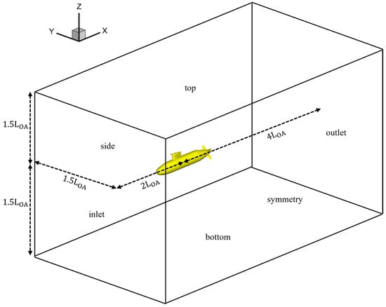
Figure 2.
Schematic of the computational domain and boundary conditions for the simulation of the Joubert BB2 submarine.
At the inlet boundary, a uniform velocity profile was imposed using the Dirichlet boundary condition for velocity and the Neumann condition for pressure. At the outlet, the Neumann condition was applied for velocity, while the Dirichlet condition was used for pressure to enable free outflow. The top, bottom, and side boundaries were treated with Neumann conditions for both velocity and pressure to simulate an unbounded fluid domain. A no-slip boundary condition was enforced on the entire submarine surface to model the viscous effects accurately.
3.3. Computational Grids
In this study, unstructured trimmed hexahedral meshes were employed to discretize the computational domain, as shown in Figure 3. The mesh was generated based on the volume-shaping strategy, with local refinement zones applied near the submarine hull and in the vicinity of the propeller plane to resolve critical flow features such as boundary layer development, vortex shedding, and wake structures. This meshing approach is consistent with best practices established in previous submarine simulations [28,29], where local volumetric refinement is crucial for accurately capturing near-wall turbulence and wake dynamics.
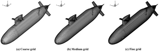
Figure 3.
Surface grid distributions on the Joubert BB2 submarine for three different grid resolutions: (a) coarse, (b) medium, and (c) fine grids.
Three different mesh resolutions were prepared to evaluate grid sensitivity: the coarse grid comprises 322,695 cells, the medium grid contains 1,098,845 cells, and the fine grid includes 2,984,274 cells. Each mesh was constructed to ensure adequate resolution near appendages, stern surfaces, and regions affected by complex flow separation. The use of trimmed cells allows for efficient control of cell quality and alignment, especially around the complex hull geometry and the X-rudder configuration, without excessive grid skewness or aspect ratio distortion. All grid levels ensure that the cell density is sufficiently high in the near-wake and propeller inflow region, which is essential for turbulence-resolving simulations.
To ensure that the near-wall resolution was appropriate for wall-function-based turbulence modeling, the non-dimensional wall distance (y⁺) was carefully evaluated. For the medium-resolution grid, the average y⁺ value near the hull surface was approximately 50, which falls within the recommended range of 30 < y⁺ < 300 suggested by the ITTC guidelines [30].
4. Results and Discussion
To assess the predictive capability of the present CFD simulations, the total resistance coefficients were compared against international benchmark data provided by multiple participating countries. The resistance coefficient is defined as follows:
where is the total resistance is the incoming flow velocity, and is the wetted surface area of the submarine model. As summarized in Table 2, the benchmark data were obtained using various CFD solvers, including Fluent (https://www.ansys.com), CFX (https://www.ansys.com), OpenFOAM (https://openfoam.org), and ReFRESCO (https://www.marin.nl) all under a consistent Reynolds number of .
Table 2.
Comparison of total resistance coefficients from various international CFD studies and the present study using the PANS and RANS models on a medium-resolution grid.
The average of the reported values was . The present simulation using the PANS model on a medium-resolution grid yielded a of , corresponding to a deviation of only from the benchmark average. In contrast, the RANS model on the same grid predicted a higher resistance coefficient of , overestimating the benchmark average by approximately . This result indicates that the RANS model tends to overpredict turbulent viscosity, thereby increasing the total resistance. In comparison, the PANS model more accurately captures the resistance behavior, supporting its suitability for high-Reynolds-number hydrodynamic simulations under moderate grid resolutions.
To further investigate the sensitivity to grid resolution, Table 3 presents the decomposition of the total resistance into pressure and viscous components for both PANS and RANS models under coarse, medium, and fine grids. For the PANS model, the total resistance shows a gradual decrease from 24.294 to 23.850 as the grid is refined, with the corresponding reducing from to . In the case of the RANS model, the total resistance remains consistently higher across all grid levels, reaching a maximum of on the fine grid.
Table 3.
Comparison of pressure, viscous, and total resistance components and corresponding total resistance coefficients for different turbulence models (PANS and RANS) and grid resolutions.
To evaluate the sensitivity of grid resolution and verify the numerical accuracy of the simulation results, a mesh convergence study was performed using the Grid Convergence Index (GCI) method introduced by Roache [31] and further formalized by Celik et al. [32] and Stern et al. [32]. The analysis focused on total resistance as the primary output metric and was conducted using three systematically refined grids: coarse, medium, and fine.
Based on the total resistance obtained from the medium and fine grids, the computed was 2.8%. According to Celik et al. [32], GCI values below 5% are generally considered acceptable for engineering-level CFD applications. Furthermore, Stern et al. [33] emphasize that sufficiently small GCI values indicate that the numerical solution resides within the asymptotic range of convergence. The GCI value obtained in this study satisfies both criteria, supporting the conclusion that the simulation results have achieved grid independence.
No significant variation in total resistance was observed with further mesh refinement, indicating that the numerical uncertainty associated with grid resolution is adequately controlled. Identical mesh configurations were applied to both the RANS and PANS simulations, ensuring that all comparative evaluations were carried out under consistent and grid-verified computational conditions.
Notably, the RANS model exhibits a stronger dependence on the viscous component of resistance, which is attributed to its higher modeled turbulent viscosity. On the other hand, the PANS model, by partially resolving turbulence, allows more realistic flow structures to develop, particularly in the near-wall and wake regions. This leads to more accurate resistance predictions with reduced sensitivity to grid-induced numerical diffusion. These findings validate the superior performance of the PANS model in capturing the total resistance characteristics and establish a robust foundation for further analysis of turbulent flow structures. In the following section, turbulent kinetic energy (TKE) distributions are examined to investigate the internal turbulence behavior that contributes to the differences in resistance prediction.
To elucidate the differences in turbulence modeling and resolution between the RANS and PANS approaches, Figure 4 presents the contours of non-dimensional turbulent kinetic energy (TKE), , in the longitudinal mid-plane for all grid resolutions. The TKE distribution directly reflects the level of modeled versus resolved turbulence, influencing the accuracy of momentum transport, wake prediction, and surface pressure recovery.
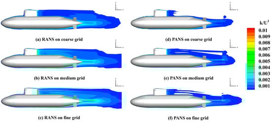
Figure 4.
Contours of non−dimensional turbulent kinetic energy (TKE) normalized by the incoming kinetic energy in the longitudinal mid-plane for RANS (left column) and PANS (right column) models using coarse, medium, and fine grids.
In the RANS simulations (Figure 4a–c), broad regions of high TKE are observed extending from the stern into the wake, particularly pronounced in the coarse and medium grids. This pattern is indicative of turbulence being entirely modeled through isotropic eddy viscosity formulations, which tend to overly diffuse the turbulent energy field. Such modeling leads to enhanced artificial mixing and momentum loss, resulting in reduced fidelity in the prediction of downstream flow features. Conversely, the PANS results (Figure 4d–f) exhibit more localized and anisotropic distributions of TKE. As the grid is refined, the PANS model reveals reduced TKE intensity and shorter wake extent, owing to its partial resolution of the turbulence spectrum. In particular, the high-TKE region in the coarse-grid RANS case (Figure 4a) extends approximately one body length downstream, maintaining a broad and diffused shape. In contrast, the corresponding region in the PANS case (Figure 4d) is significantly narrower and diminishes more rapidly, indicating reduced reliance on modeled turbulence. The fine-grid results (Figure 4c,f) further highlight this trend, as the RANS solution retains extended turbulent energy in the wake, whereas the PANS model confines TKE closer to the body, reflecting increased turbulence resolution near the hull surface and in the immediate wake zone. The ability of the PANS formulation to dynamically adjust the modeled-to-resolved turbulence ratio leads to a more realistic representation of flow unsteadiness and energy dissipation mechanisms. Importantly, this reduction in modeled turbulent viscosity minimizes numerical diffusion and supports the development of sharper velocity gradients and more coherent flow structures.
To further examine how the adaptive behavior of the PANS model responds to grid resolution, Figure 5 presents the spatial distribution of the resolution control parameter in the longitudinal mid-plane for the coarse, medium, and fine PANS simulations. In the dynamic PANS framework [26], is defined as the ratio of unresolved to total turbulent kinetic energy ), and governs the extent to which turbulence is modeled versus resolved. A value of corresponds to a fully modeled RANS-like state, while lower values indicate that a greater portion of turbulence is resolved. Because is locally evaluated based on the flow scale and grid size, it serves as a spatially varying indicator of turbulence resolution within the domain.
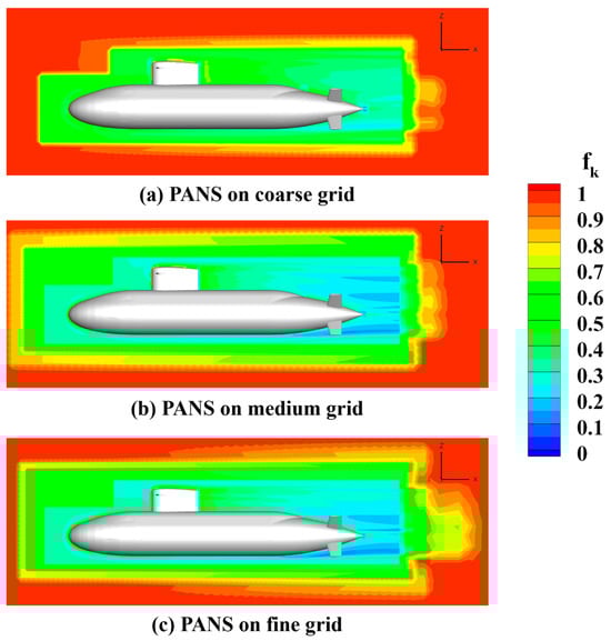
Figure 5.
Contours of estimated resolution control parameter in the longitudinal mid-plane for PANS simulations using coarse, medium, and fine grids.
For the coarse-grid case (Figure 5a), remains close to 1 throughout most of the domain, especially around the hull and in the near-wake region, implying that turbulence is predominantly modeled and fine-scale vortices are not resolved. This is particularly evident near the sail and stern appendages, where high values reflect a reduced capacity to capture anisotropic vortex shedding and unsteady separation. Consequently, the flow structures in these regions are dominated by numerical diffusion, which aligns with the broad and smeared TKE distributions shown in Figure 4.
As the grid is refined to the medium-resolution (Figure 5b), noticeable reductions in appear around the rudder and stern, with values decreasing to approximately 0.4–0.6. This suggests that the PANS model begins to resolve more turbulent fluctuations in regions that are critical for wake development and pressure recovery. A similar decrease is observed around the sail, indicating improved resolution of unsteady vortex dynamics and tip separation.
In the fine-grid case (Figure 5c), the impact of resolution control becomes most apparent, with localized zones of near the stern, sail, and propeller hub. These low- values suggest that the PANS model operates in a LES-like mode in these high-shear and vortex-active regions. Additionally, the contraction of high- areas in the wake region reflects enhanced capture of shear-layer structures and energy dissipation mechanisms driven by grid refinement. This trend is consistent with the earlier TKE results, confirming that the dynamic PANS method self-adjusts turbulence resolution in response to local flow and grid conditions.
The progressive reduction in with grid refinement highlights the self-adaptive capability of the PANS model. In critical areas such as the sail, rudder, and stern, lower values enable a more physically realistic representation of anisotropic turbulent structures. This improved resolution plays a critical role in predicting pressure recovery, wake coherence, and resistance components with greater reliability, as will be discussed in the following sections.
Building on the observed differences in turbulence intensity, Figure 6 presents the surface pressure coefficient distribution along with streamlines to evaluate the impact of turbulence modeling on pressure-induced resistance. The pressure coefficient is defined as follows:
where and denote the local and reference pressures, respectively. Since pressure gradients and flow separation—particularly in the stern region—are highly sensitive to turbulence modeling, a detailed examination of this area provides critical insights into drag characteristics. Thus, only the aft portion of the hull is magnified in Figure 6, where the most pronounced discrepancies are observed.
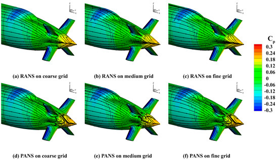
Figure 6.
Surface pressure coefficient distribution and streamlines on the hull for RANS (top row) and PANS (bottom row) using coarse, medium, and fine grids.
Across all grid resolutions, RANS simulations (Figure 6a–c) exhibit broader low-pressure zones near the stern’s upper and lower surfaces, suggesting intensified adverse pressure gradients and premature separation. In coarse and medium grids, streamlines deviate significantly from the hull surface, indicating early detachment and formation of recirculation zones. These phenomena are consistent with the elevated turbulent kinetic energy shown in Figure 4, where the excessive eddy viscosity in RANS leads to over-diffusion of momentum, resulting in degraded pressure recovery and higher pressure resistance. In contrast, the PANS model (Figure 6d–f) yields more localized and smoother pressure gradients, particularly for medium and fine grids. The streamlines remain attached closer to the hull surface and extend farther downstream, implying delayed separation and enhanced flow alignment. This improvement is attributed to the PANS model’s scale-resolving capability, which reduces artificial turbulent viscosity and captures anisotropic flow features more accurately. Moreover, the surface pressure distribution in the aft-body region indicates that the PANS model achieves a more effective pressure recovery, particularly near the propeller hub and stern taper. In these areas, the pressure coefficient values increase more gradually toward the trailing edge, reflecting a smoother redistribution of pressure. In contrast, RANS simulations show persistently low values over a broader area, which implies insufficient momentum recovery and increased pressure drag. These observations highlight the PANS model’s capability to resolve adverse pressure gradients more accurately, especially under refined grid conditions. As a result, pressure-induced resistance in the aft body—especially in the vicinity of control surfaces and the propeller hub—is significantly mitigated. These results affirm that accurate turbulence resolution not only reduces pressure losses but also preserves flow coherence in critical regions, offering direct benefits in total resistance prediction. The subsequent section examines wall shear stress distributions to further evaluate viscous effects under both modeling approaches.
While pressure drag is dominant in the aft-body region, viscous resistance remains a significant contributor to the total resistance, particularly in the boundary layer development along the hull. Figure 7 illustrates the distribution of the non-dimensional wall shear stress coefficient, defined as follows:
where denotes the wall shear stress. The contour maps allow for a direct comparison of near-wall flow behavior between RANS and PANS models under varying grid resolutions.
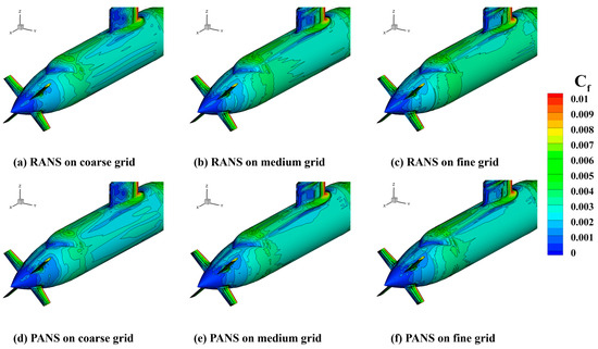
Figure 7.
Non−dimensional wall shear stress distribution on the hull surface for RANS (top row) and PANS (bottom row) using coarse, medium, and fine grids.
In RANS simulations (Figure 7a–c), the wall shear stress levels are notably higher across the lower stern and sail appendages, with increased intensity as grid resolution improves. This trend reflects the RANS model’s tendency to overpredict turbulent viscosity, leading to artificially thickened boundary layers and excessive shear. The broadened high- regions correlate with the elevated TKE levels previously observed in Figure 4, reinforcing the pattern of excessive modeled turbulence and its impact on viscous resistance. However, PANS simulations (Figure 7d–f) exhibit more localized and moderated distributions, suggesting thinner and more physically realistic boundary layers. Particularly near appendage junctions and the propeller hub region, the PANS model yields reduced wall shear stress magnitudes. Furthermore, along the mid-body section of the hull, the RANS model predicts an extended region of elevated , particularly under fine-grid conditions. This trend suggests an overestimation of boundary layer thickness and shear buildup along the longitudinal hull surface. In contrast, the PANS model limits this shear accumulation, maintaining more moderate levels across the same region. These observations reaffirm the capability of the PANS model to better resolve near-wall turbulence, particularly with refined grids, and we sincerely appreciate the reviewer’s suggestion that guided us to strengthen this comparison. This is attributed to its scale-resolving nature, which partially resolves near-wall turbulence structures and suppresses the over-diffusion of momentum inherent to fully modeled approaches. The resulting flow field better captures anisotropic shear-layer development and yields a more accurate estimation of viscous drag forces. Overall, these results demonstrate that the PANS model provides a more balanced and physically accurate treatment of near-wall turbulence. Notably, the medium-resolution grid achieves a favorable compromise between computational efficiency and accuracy, making PANS particularly well suited for practical viscous flow predictions in full-scale simulations.
The combined influence of pressure and viscous forces ultimately manifests in the streamwise momentum transport characteristics, visualized in Figure 8 through cross-sectional velocity contours normalized by the inflow velocity . These distributions allow for direct assessment of boundary layer thickness, wake symmetry, and momentum deficit across the hull length, particularly in the stern and propeller regions.
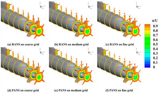
Figure 8.
Normalized streamwise velocity distribution on cross−sectional slices along the hull for RANS (top row) and PANS (bottom row) using coarse, medium, and fine grids.
In the RANS simulations (Figure 8a–c), the wake exhibits a broad, axisymmetric low-speed core with an extended region of velocity deficit near the propeller hub. The wake spreads radially with increasing grid refinement yet consistently displays signs of excessive turbulent diffusion. This behavior aligns with the elevated TKE and wall shear stress previously observed, indicating strong artificial mixing and rapid momentum dissipation. The resulting velocity profiles show diminished core flow retention and a thicker wake envelope, which adversely affects wake recovery and increases overall form drag. By contrast, the PANS simulations (Figure 8d–f) generate a narrower, more coherent wake structure with sharper velocity gradients and improved momentum conservation along the centerline. The wake region remains more compact and retains higher axial velocity, suggesting reduced artificial turbulent diffusion and more accurate resolution of shear layers. These characteristics are especially apparent in the medium and fine grids, where the PANS model effectively preserves unsteady structures and better captures the physics of wake evolution. The observed improvements in momentum transport confirm the PANS model’s capability to more accurately simulate wake development, which is critical for both propulsion performance evaluation and resistance estimation. In particular, the delayed wake thickening and improved core flow retention explain the reduced total resistance values reported in earlier sections.
To further evaluate the influence of turbulence modeling on the wake structure, Figure 9 presents cross-sectional contours of normalized axial velocity in the propeller plane, taken approximately one diameter downstream of the stern. These contours are crucial for understanding the wake deficit profile, which significantly affects propeller inflow uniformity and overall propulsion efficiency.
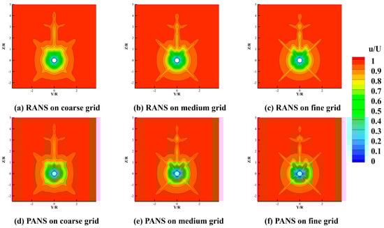
Figure 9.
Cross−sectional contours of the normalized axial velocity component in the propeller plane RANS (top row) and PANS (bottom row) using coarse, medium, and fine grids.
Across all grid resolutions, the RANS simulations (Figure 9a–c) produce nearly axisymmetric wake profiles with a pronounced central velocity deficit. The deficit region appears broad and gradually recovering in the radial direction, especially in the coarse and medium grid cases. This smooth and diffused wake structure is indicative of excessive turbulent viscosity, consistent with the high TKE fields seen in Figure 4. Such artificial diffusion leads to smeared velocity gradients, suppressing the development of coherent wake features and underrepresenting the effects of shear-layer instabilities and appendage-induced vortices. In contrast, the PANS model (Figure 9d–f) exhibits more compact, anisotropic wake profiles with sharper velocity gradients. As the grid is refined, the axial velocity contours show a distinct narrowing of the deficit region and clearer delineation of high-shear zones near appendages. These features, especially visible in the fine-grid case (Figure 9f), reflect the improved scale-resolving capabilities of the PANS approach. By allowing partial resolution of turbulence, PANS better preserves axial momentum and captures the localized flow features critical for accurate prediction of propeller inflow conditions.
To quantify the azimuthal variations in wake velocity, Figure 10 shows the circumferential distribution of normalized axial velocity at four radial locations in the propeller plane. These radial cuts offer detailed comparisons against RANS-based international benchmark datasets from Canada (CAN), Germany (D), France (F), and The Netherlands (NL).

Figure 10.
Circumferential distribution of normalized axial velocity component at four radial positions (r/R = 0.65, 0.75, 0.95, 1.05) on the propeller plane.
The RANS results (solid lines) show good agreement with the reference data, particularly on the fine grid, confirming the numerical accuracy and consistency of the current simulation framework. The profiles capture key wake features such as local velocity dips and peaks caused by hull appendages and separation zones. These consistent patterns validate the RANS model’s capability to replicate the gross wake characteristics typically captured by traditional RANS-based studies. On the other hand, the PANS results (dashed lines) exhibit more pronounced azimuthal variation and lower axial velocity in regions near the centerline (notably at and ). These deviations are not errors but rather consequences of resolving finer turbulent structures. Unlike RANS, which fully models all turbulence, PANS resolves part of the spectrum, enabling the capture of sharper shear layers and fluctuating flow features. This results in enhanced detection of wake asymmetries and flow unsteadiness that is otherwise smeared out in fully modeled approaches.
At higher radial positions ( and ), the differences between RANS and PANS diminish, indicating that outer wake regions are governed more by large-scale flow features and less by turbulence modeling details. The convergence of results in these regions supports the notion that PANS provides added value primarily in capturing inner-wake complexity. Together, Figure 9 and Figure 10 illustrate that while RANS delivers results in line with traditional benchmarks, the PANS model yields improved fidelity in wake resolution, especially in the near-axis region where flow gradients are strongest. These insights underscore the advantage of using PANS for high-resolution propeller inflow analysis and reinforce its potential for enhanced wake-adaptive propulsion simulations.
To qualitatively assess the flow coherence and three-dimensional vortex dynamics, Figure 11 presents iso-surfaces of the Q-criterion for both RANS and PANS simulations at coarse-, medium-, and fine-grid resolutions. The Q-criterion, defined as the second invariant of the velocity gradient tensor, is commonly employed to extract rotationally dominated regions in turbulent flows and thereby identify coherent vortex structures.
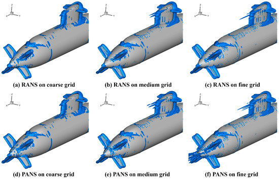
Figure 11.
Iso−surfaces of the Q−criterion colored by vorticity magnitude for RANS (top row) and PANS (bottom row) simulations using coarse, medium, and fine grids.
In the RANS simulations (Figure 11a–c), the identified vortices appear sparse, fragmented, and primarily concentrated near the wall boundaries. Even with fine-grid resolution, the captured structures are relatively short and lack spatial continuity—particularly around critical flow control regions such as the sail, rudder, and stern appendages. This limitation stems from the RANS model’s reliance on fully modeled turbulence and isotropic eddy viscosity assumptions, which inherently suppress the resolution of fine-scale vortical features. Consequently, only large-scale, diffused vortical patterns are captured, limiting the model’s capacity to resolve shear-layer instabilities or trailing vortex dynamics. In contrast, the PANS simulations (Figure 11d–f) reveal substantially more detailed and elongated vortex structures, which exhibit greater spatial coherence and physical realism. Even at medium grid resolution, the PANS model captures tip vortices from the sail, trailing vortices from stern appendages, and wake-induced shear-layer roll-up phenomena that are underrepresented or absent in the RANS solutions. These enhanced flow structures result from the PANS model’s ability to partially resolve the turbulence spectrum, allowing it to reproduce anisotropic eddies and complex flow interactions that contribute to accurate wake and resistance predictions.
Notably, in the medium grid case (Figure 11b vs. Figure 11e), the PANS model resolves secondary vortex interactions and streamwise-aligned coherent structures near the propeller hub and stern planes—features completely missed by the RANS counterpart. This suggests that PANS delivers LES-like resolution characteristics on intermediate grids, offering a favorable trade-off between computational cost and flow fidelity. The higher spatial resolution and continuity of vortical features observed in the PANS simulations strongly support earlier field-based observations in the TKE, pressure, and velocity analyses. Together, these results affirm that PANS not only improves the quantitative accuracy of resistance prediction but also enhances the physical interpretability of flow features critical for assessing wake integrity, propeller inflow non-uniformity, and appendage-induced instabilities.
5. Summary and Conclusions
In this study, a comparative computational analysis was conducted to evaluate the performance of the Reynolds-averaged Navier–Stokes (RANS) and Partially averaged Navier–Stokes (PANS) turbulence models for simulating the flow around the Joubert BB2 submarine in calm-water conditions. The primary objective was to assess how differences in turbulence resolution affect resistance prediction, wall-boundary behavior, and wake development, particularly in relation to grid sensitivity. To this end, three levels of grid resolution—coarse, medium, and fine—were constructed using unstructured trimmed hexahedral meshes with local refinement applied near the stern and appendages. Both turbulence models were applied using an identical computational setup, and the resulting simulations were validated against internationally recognized RANS-based datasets.
The results revealed that the PANS model consistently produced improved predictions of total resistance, particularly on medium and fine grids, by reducing excessive turbulent viscosity commonly observed in RANS simulations. Specifically, the PANS model yielded resistance values closely aligned with benchmark data, while the RANS model tended to overestimate drag due to premature flow separation and artificially diffused turbulent stresses. Analysis of the surface pressure coefficient and wall shear stress distributions showed that RANS produced broader low-pressure zones and higher shear magnitudes near the stern, indicating strong adverse pressure gradients and thickened boundary layers. In contrast, PANS more accurately captured localized pressure recovery and thinner, more physically realistic boundary layer development. These trends were further supported by the turbulent kinetic energy (TKE) distributions, where PANS predicted more confined and anisotropic turbulence fields that better preserved momentum and limited turbulent diffusion in the stern region. In addition, the grid-dependent variation of the resolution control parameter provided further insight into the adaptive behavior of the PANS model. As the grid was refined, values systematically decreased in critical flow regions such as the sail, rudder, and stern appendages. This reduction corresponded to increased turbulence resolution and aligned with observed improvements in pressure recovery, boundary layer definition, and wake coherence. In terms of wake dynamics, PANS demonstrated its superiority by resolving a narrower, more coherent wake profile with higher centerline velocities and sharper shear-layer gradients. Cross-sectional velocity fields and circumferential distributions at the propeller plane further illustrated that PANS captured greater asymmetry and more refined turbulent structures than RANS, which tended to produce a broadened and homogenized inflow. This fidelity in wake resolution is particularly advantageous for propeller–hull interaction analysis and cavitation prediction. The advantages of PANS were also evident in the vortex structure analysis using Q-criterion iso-surfaces. The model successfully identified coherent vortices originating from the sail, rudders, and appendages, whereas RANS failed to resolve these structures with sufficient detail, especially at lower grid resolutions. The enhanced resolution of unsteady vortical features in PANS suggests its capability to simulate complex submarine wake behavior without requiring the computational expense of full LES.
Overall, the findings of this study demonstrate that the PANS turbulence model provides a favorable compromise between accuracy and computational cost. When combined with moderate mesh refinement, PANS significantly improves the prediction of resistance components, pressure and shear fields, and wake dynamics compared to conventional RANS. These results support the use of PANS as a practical and effective turbulence modeling approach for submarine CFD simulations, especially in contexts where LES is computationally prohibitive. Future studies will extend the present framework to self-propelled configurations, unsteady maneuvers, and cavitating flow conditions to further explore the applicability of the PANS approach in realistic naval hydrodynamics.
Author Contributions
Conceptualization, W.S.; Methodology, H.L.; Software, C.L.; Validation, C.L.; Investigation, C.L., H.L. and W.S.; Data curation, H.L.; Writing—original draft, C.L.; Writing—review & editing, W.S.; Visualization, H.L.; Supervision, W.S. All authors have read and agreed to the published version of the manuscript.
Funding
This work was supported by a grant from Brain Korea 21 Program for Leading Universities and Students (BK21 FOUR) MADEC Marine Designeering Education Research Group. This work was also supported by the Korea Institute for Advancement of Technology (KIAT) grant funded by the Korea Government (MOTIE) (RS-2025-02263945, HRD Program for Industrial Innovation).
Data Availability Statement
The raw data supporting the conclusions of this article will be made available by the authors upon request.
Conflicts of Interest
The authors declare no conflict of interest.
References
- Kim, D.-H.; Kim, Y.; Baek, H.-M.; Choi, Y.-M.; Kim, Y.J.; Park, H.; Yoon, H.K.; Shin, J.-H.; Lee, J.; Chae, E.J.; et al. Experimental study of the hydrodynamic maneuvering coefficients for a BB2 generic submarine using the planar motion mechanism. Ocean Eng. 2023, 271, 113428. [Google Scholar] [CrossRef]
- Kim, D.-H.; Kim, J.; Baek, H.-M.; Choi, Y.-M.; Shin, J.-H.; Lee, J.; Shin, S.-C.; Shin, Y.-H.; Chae, E.J.; Kim, E.S.; et al. Experimental investigation on a generic submarine hydrodynamic model considering the interaction effects of hull motion states and control planes. Ocean Eng. 2024, 298, 116878. [Google Scholar] [CrossRef]
- Chen, M.; Zhang, N.; Zheng, W.; Li, Y. Numerical simulation of near-surface turn maneuver of a generic submarine. Ocean Eng. 2023, 287, 115835. [Google Scholar] [CrossRef]
- Dogrul, A. Numerical prediction of scale effects on the propulsion performance of Joubert BB2 submarine. Brodo-Gradnja Int. J. Nav. Archit. Ocean. Eng. Res. Dev. 2022, 73, 17–42. [Google Scholar]
- Park, J.; Seok, W. Computational analysis of strut effects on a BB2 submarine at drift angle 0, 6, and 12°. Int. J. Nav. Arch. Ocean Eng. 2023, 15, 100555. [Google Scholar] [CrossRef]
- Rocca, A.; Cianferra, M.; Broglia, R.; Armenio, V. Computational hydroacoustic analysis of the BB2 submarine using the advective Ffowcs Williams and Hawkings equation with Wall-Modeled LES. Appl. Ocean Res. 2022, 129, 103360. [Google Scholar] [CrossRef]
- Chen, M.; Zhang, N.; Sun, H.; Zhang, X. Large Eddy Simulation of the Flow around a Generic Submarine under Straight-Ahead and 10° Yaw Conditions. J. Mar. Sci. Eng. 2023, 11, 2286. [Google Scholar] [CrossRef]
- Huong, Y.T.; Leong, Z.Q.; Conway, A.; Duffy, J.; Ranmuthugala, D. Downstream wake features of a Rood wing predicted by different turbulence models. J. Mar. Sci. Technol. 2024, 29, 725–744. [Google Scholar] [CrossRef]
- Liefvendahl, M.; Fureby, C. Grid requirements for LES of ship hydrodynamics in model and full scale. Ocean Eng. 2017, 143, 259–268. [Google Scholar] [CrossRef]
- Ouvrard, H.; Koobus, B.; Dervieux, A.; Salvetti, M.V. Classical and variational multiscale LES of the flow around a circular cylinder on unstructured grids. Comput. Fluids 2010, 39, 1083–1094. [Google Scholar] [CrossRef]
- Nisham, A.; Terziev, M.; Tezdogan, T.; Beard, T.; Incecik, A. Prediction of the aerodynamic behaviour of a full-scale naval ship in head waves using Detached Eddy Simulation. Ocean Eng. 2021, 222, 108583. [Google Scholar] [CrossRef]
- Ren, Z.; Wang, J.; Wan, D. Investigation of fine viscous flow fields in ship planar motion mechanism tests by DDES and RANS methods. Ocean Eng. 2022, 243, 110272. [Google Scholar] [CrossRef]
- Zhang, J.; Gidado, F.; Adamu, A.; Guo, Z.; Gao, G. An investigation on the wake flow of a generic ship using IDDES: The effect of computational parameters. Ocean Eng. 2023, 271, 113644. [Google Scholar] [CrossRef]
- Girimaji, S.S. Partially-averaged Navier-Stokes model for turbulence: A Reynolds-averaged Navier-Stokes to direct numerical simulation bridging method. J. Appl. Mech. 2005, 73, 413–421. [Google Scholar] [CrossRef]
- Zhang, J.; Minelli, G.; Rao, A.N.; Basara, B.; Bensow, R.; Krajnović, S. Comparison of PANS and LES of the flow past a generic ship. Ocean Eng. 2018, 165, 221–236. [Google Scholar] [CrossRef]
- Bensow, R.E.; van den Boogaard, M. Using a PANS simulation approach for the transient flow around the Japan Bulk Carrier. J. Ship Res. 2019, 63, 123–129. [Google Scholar] [CrossRef]
- Ji, B.; Luo, X.; Wu, Y.; Peng, X.; Xu, H. Partially-Averaged Navier–Stokes method with modified k–ε model for cavi-tating flow around a marine propeller in a non-uniform wake. Int. J. Heat Mass Transf. 2012, 55, 6582–6588. [Google Scholar] [CrossRef]
- Kamble, C.; Girimaji, S. Characterization of coherent structures in turbulent wake of a sphere using partially averaged Navier–Stokes (PANS) simulations. Phys. Fluids 2020, 32, 105110. [Google Scholar] [CrossRef]
- Menter, F.R. Influence of freestream values on k-omega turbulence model predictions. AIAA J. 1992, 30, 1657–1659. [Google Scholar] [CrossRef]
- Menter, F.R. Two-equation eddy-viscosity turbulence models for engineering applications. AIAA J. 1994, 32, 1598–1605. [Google Scholar] [CrossRef]
- Menter, F.R. Eddy viscosity transport equations and their relation to the k-ε model. J. Fluids Eng. 1997, 119, 876–884. [Google Scholar] [CrossRef]
- Lakshmipathy, S.; Girimaji, S. Partially-averaged Navier-Stokes method for turbulent flows: k-w model implementation. In Proceedings of the 44th AIAA Aerospace Sciences Meeting and Exhibit, Reno, NA, USA, 9–12 January 2006; p. 119. [Google Scholar]
- Alfonsi, G. Reynolds-averaged Navier–Stokes equations for turbulence modeling. Appl. Mech. Rev. 2009, 62, 040802. [Google Scholar] [CrossRef]
- Pereira, F.S.; Vaz, G.; Eça, L. An assessment of scale-resolving simulation models for the flow around a circular cyl-inder. In Proceedings of the 8th International Symposium on Turbulence, Heat and Mass Transfer (THMT15), Sarajevo, Bosnia and Herzegovina, 15–18 September 2015; pp. 295–298. [Google Scholar]
- Seok, W.; Lee, S.B.; Rhee, S.H. An improved partially-averaged Navier-Stokes model for secondary flows. Int. J. Heat Mass Transf. 2021, 180, 121780. [Google Scholar] [CrossRef]
- Luo, D.; Yan, C.; Liu, H.; Zhao, R. Comparative assessment of PANS and DES for simulation of flow past a circular cylinder. J. Wind. Eng. Ind. Aerodyn. 2014, 134, 65–77. [Google Scholar] [CrossRef]
- Broglia, R.; Posa, A.; Bettle, M.C. Analysis of vortices shed by a notional submarine model in steady drift and pitch advancement. Ocean Eng. 2020, 218, 108236. [Google Scholar] [CrossRef]
- Toxopeus, S.L. SHWG collaborative exercise: BB2. In Technology Report 26053–9-RD; Marin: Wageningen, The Netherlands, 2016. [Google Scholar]
- Wang, W.; Chen, Y.; Xia, Y.; Xu, G.; Zhang, W.; Wu, H. A fault-tolerant steering prototype for x-rudder underwater vehicles. Sensors 2020, 20, 1816. [Google Scholar] [CrossRef] [PubMed]
- ITTC. 7.5-03-02-03 Practical Guidelines for Ship CFD Applications. In ITTC—Recommended Procedures and Guidelines; ITTC: Pune, Maharashtra, 2014. [Google Scholar]
- Roache, P.J. Perspective: A method for uniform reporting of grid refinement studies. ASME J. Fluids Eng. 1994, 116, 405–413. [Google Scholar] [CrossRef]
- Celik, I.B.; Ghia, U.; Roache, P.J.; Freitas, C.J. Procedure for estimation and reporting of uncertainty due to dis-cretization in CFD applications. J. Fluids Eng.-Trans. ASME 2008, 130, 078001. [Google Scholar]
- Stern, F.; Wilson, R.V.; Coleman, H.W.; Paterson, E.G. Comprehensive approach to verification and validation of CFD simulations—Part 1: Methodology and procedures. J. Fluids Eng. 2001, 123, 793–802. [Google Scholar] [CrossRef]
Disclaimer/Publisher’s Note: The statements, opinions and data contained in all publications are solely those of the individual author(s) and contributor(s) and not of MDPI and/or the editor(s). MDPI and/or the editor(s) disclaim responsibility for any injury to people or property resulting from any ideas, methods, instructions or products referred to in the content. |
© 2025 by the authors. Licensee MDPI, Basel, Switzerland. This article is an open access article distributed under the terms and conditions of the Creative Commons Attribution (CC BY) license (https://creativecommons.org/licenses/by/4.0/).