
Triaxial Experimental Study of Natural Gas Hydrate Sediment Fracturing and Its Initiation Mechanisms: A Simulation Using Large-Scale Ice-Saturated Synthetic Cubic Models

 ,
,
Abstract
1. Introduction
2. Experimental Methods
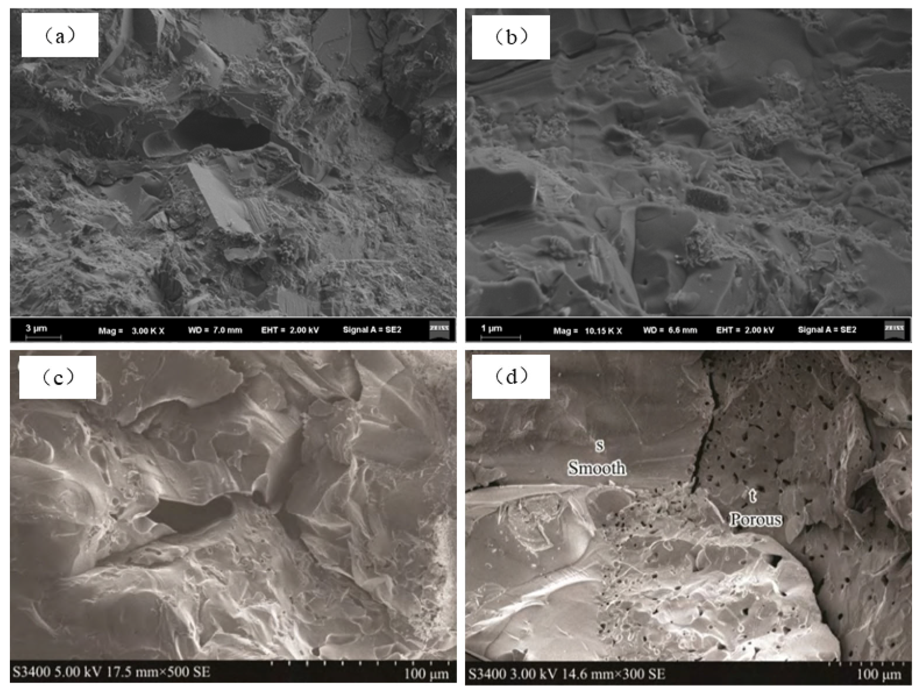
2.1. Experimental Materials
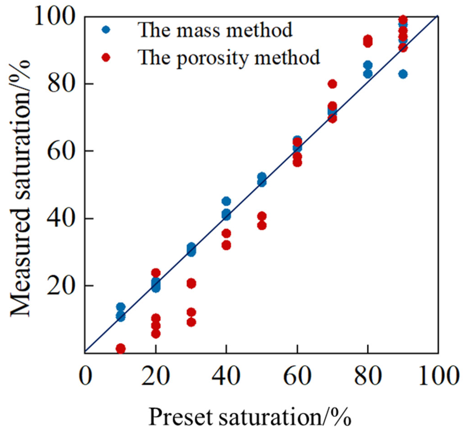
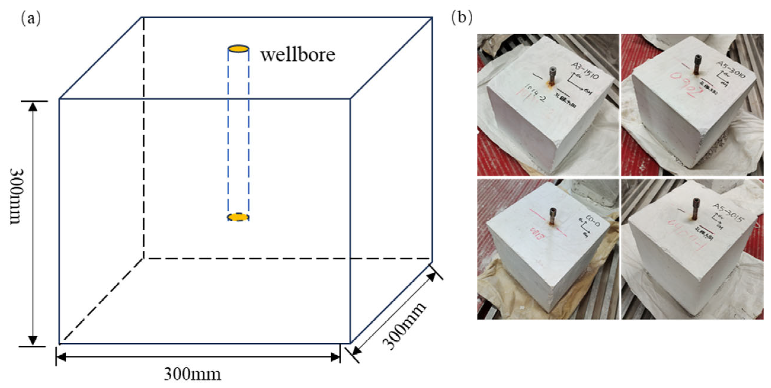
2.2. Sample Preparation
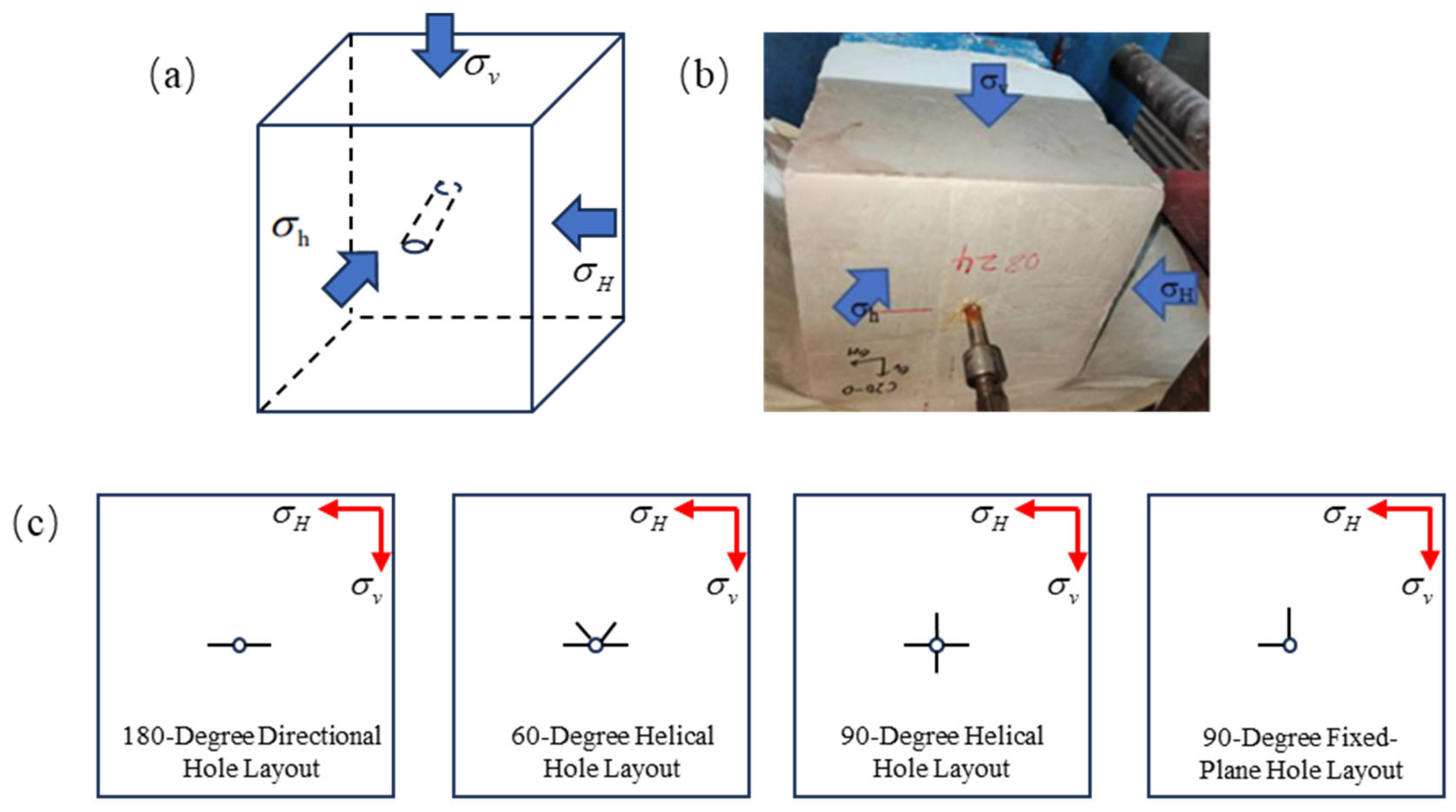
2.3. Experimental Device and Procedure
2.4. Experimental Design
3. Experiment Results and Analysis
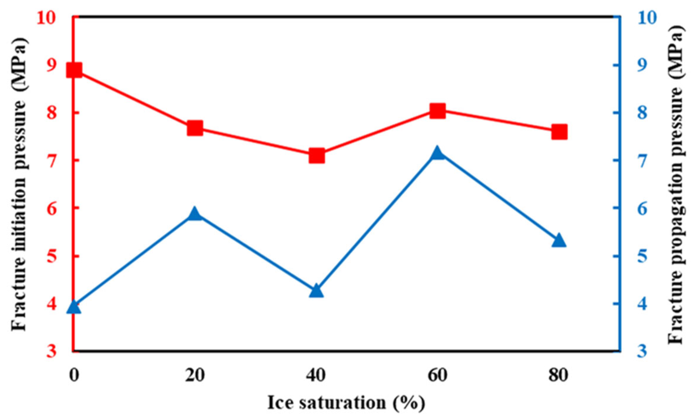
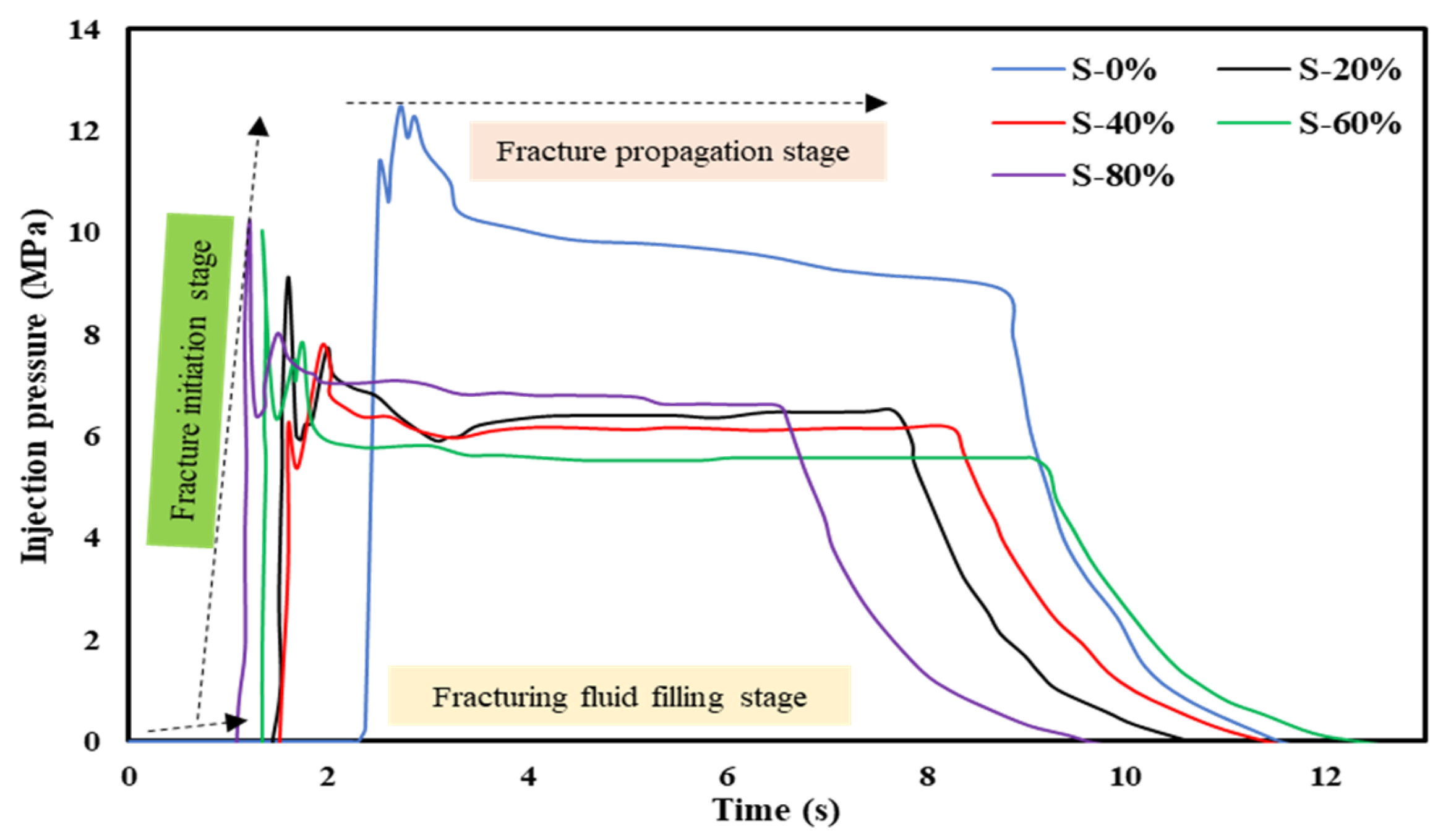
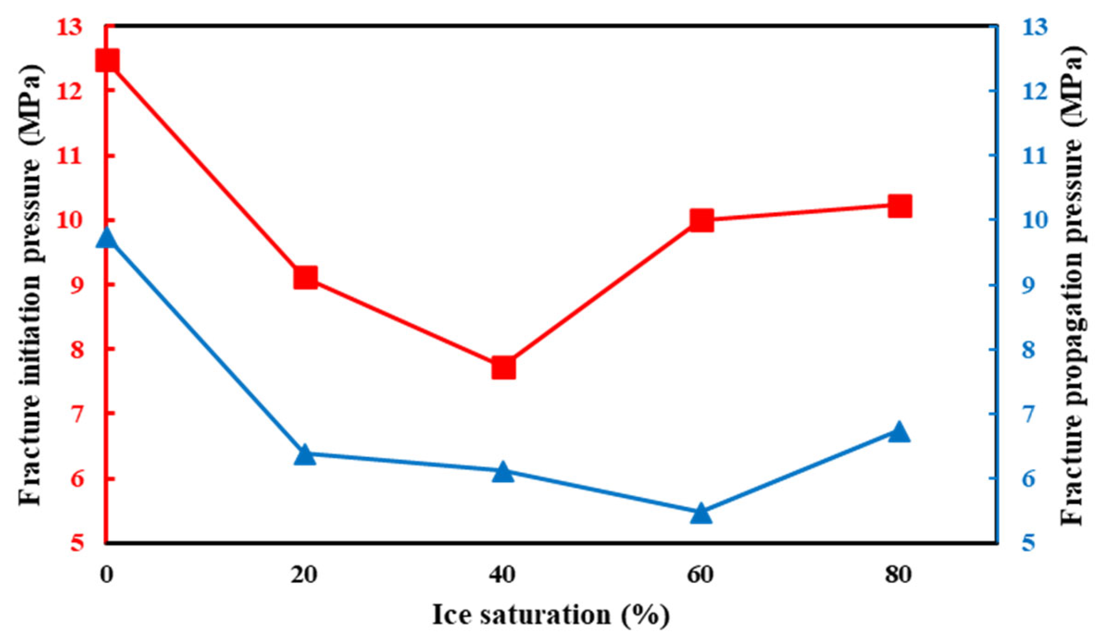
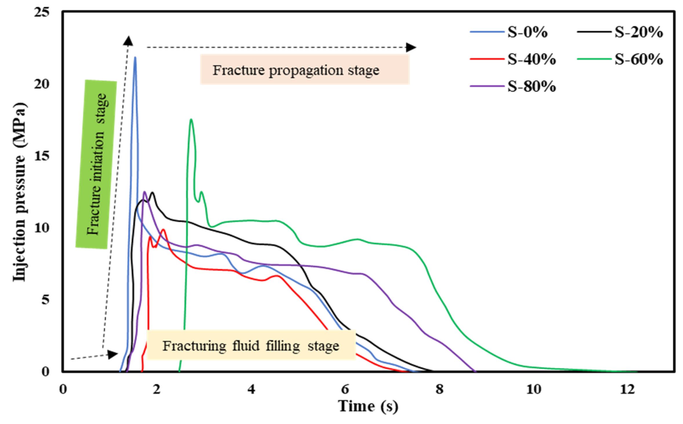
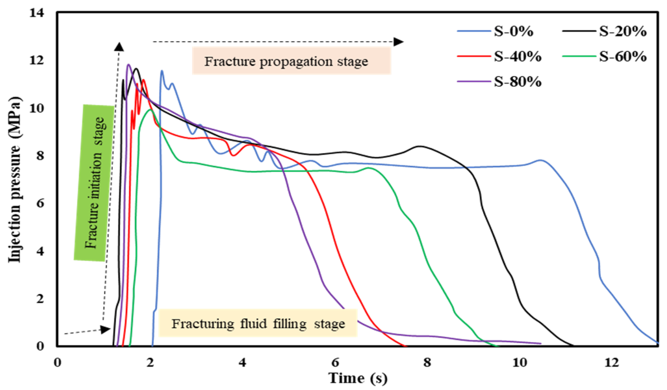
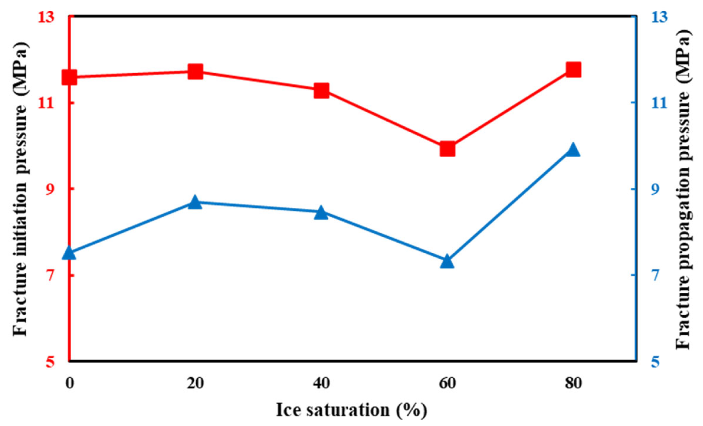
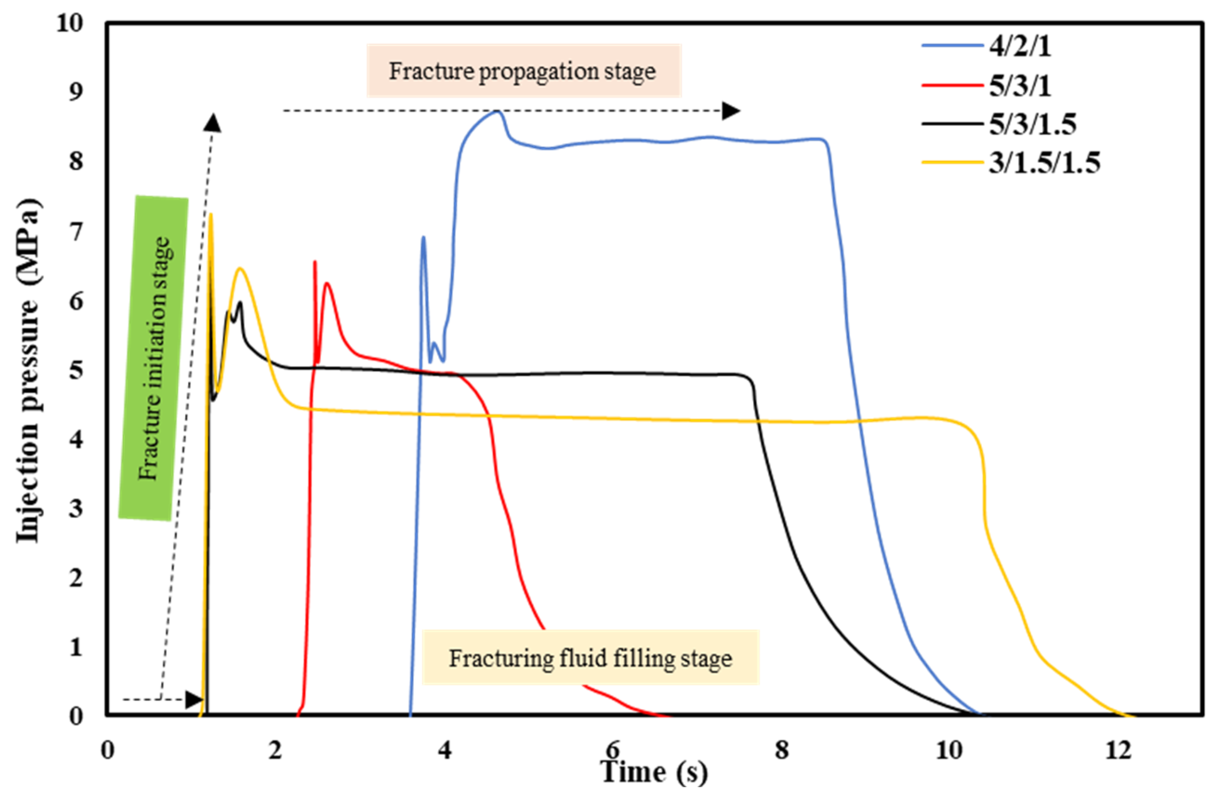
3.1. Effect of Ice Saturation and Fracturing Fluid Viscosity
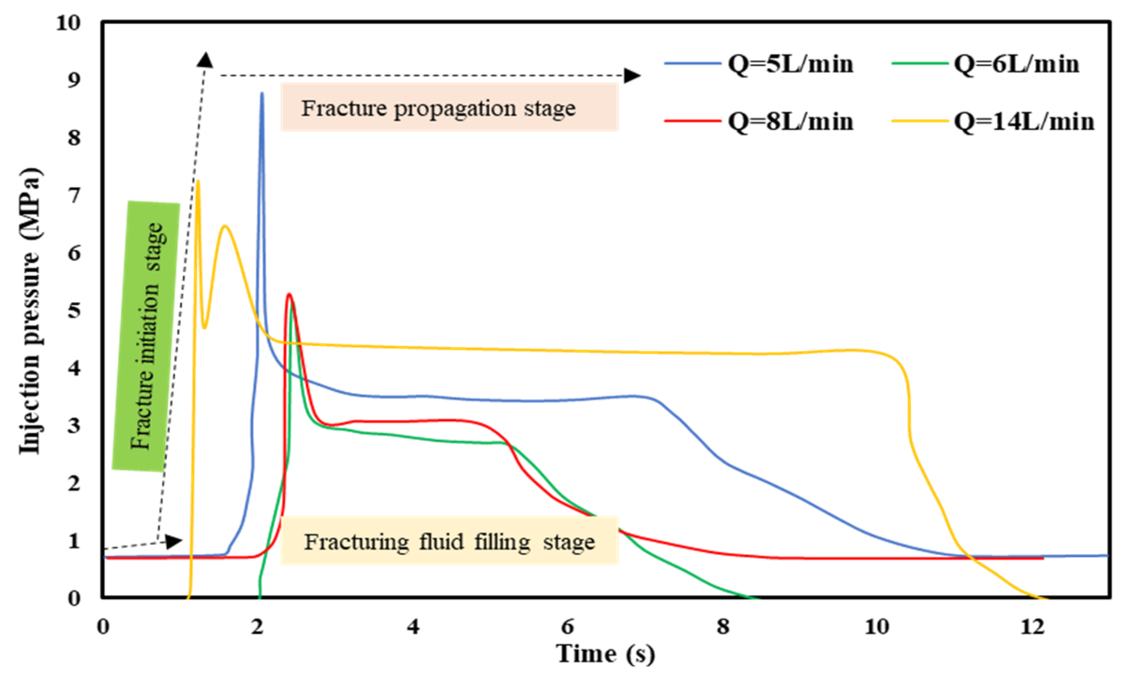
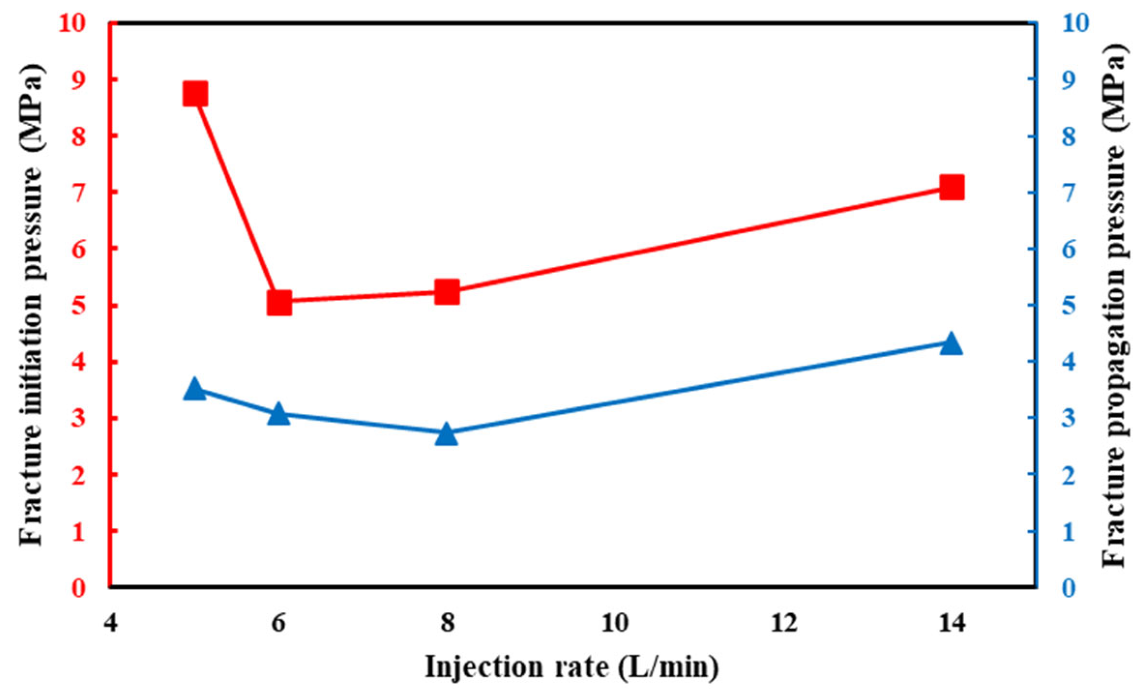
3.2. Effect of Injection Rate
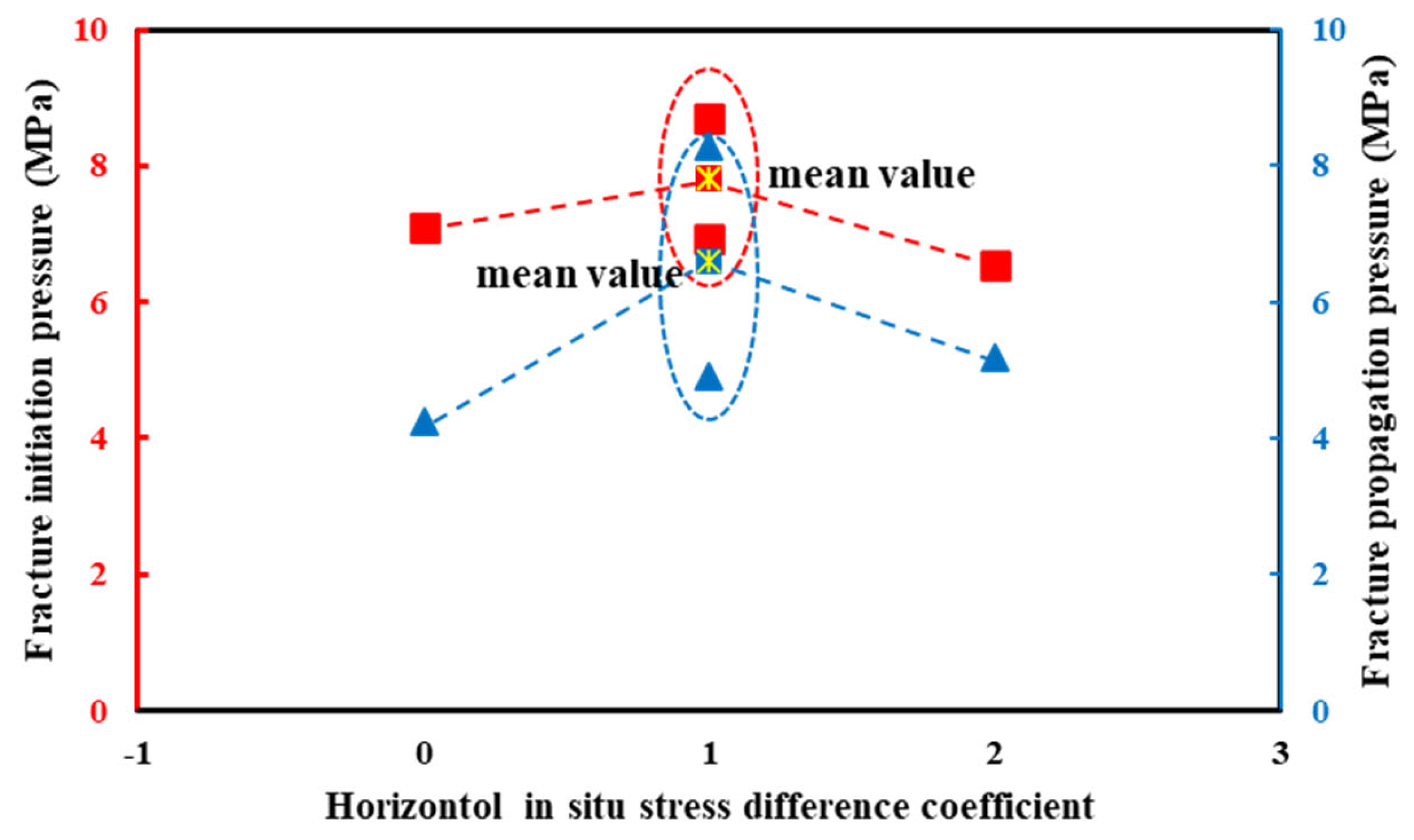
3.3. Effect of Horizontal In Situ Stress Difference
3.4. Effect of Perforation Patterns
4. Discussion
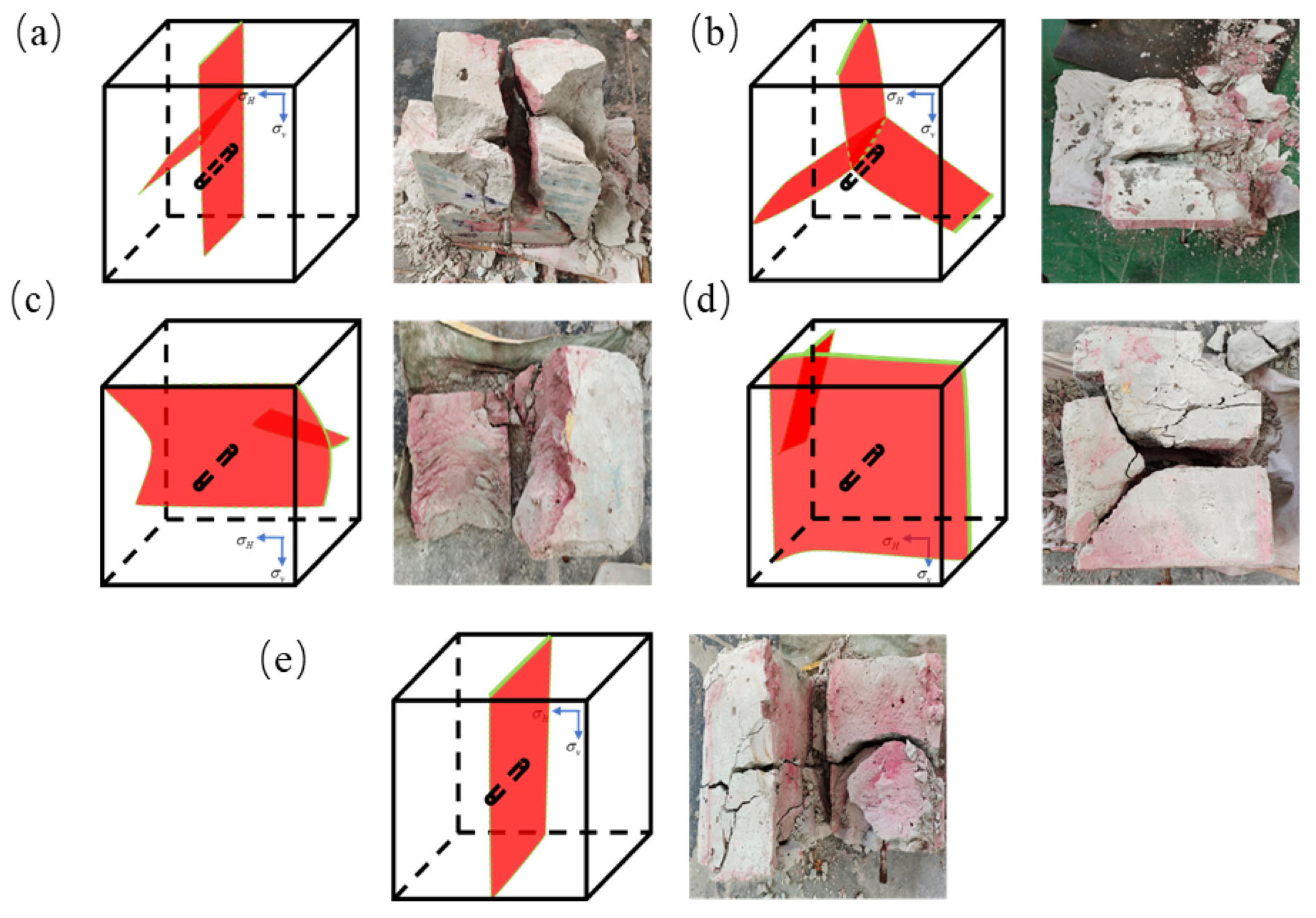
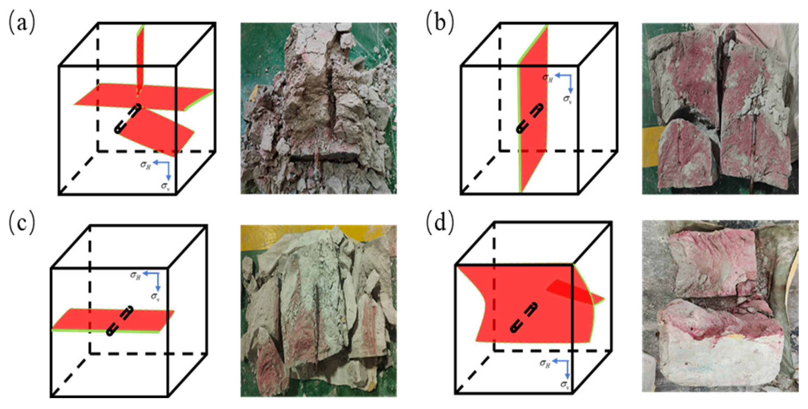
4.1. Analysis of Fracture Morphology During Hydraulic Fracturing
4.2. Hydrate Constitutive Model and Fitting
4.2.1. Nonlinear Constitutive Equation for Hydrate Sediments
4.2.2. Total Deformation Theory
4.2.3. Sensitivity Analysis of Elastic–Plastic Constitutive Model Parameters
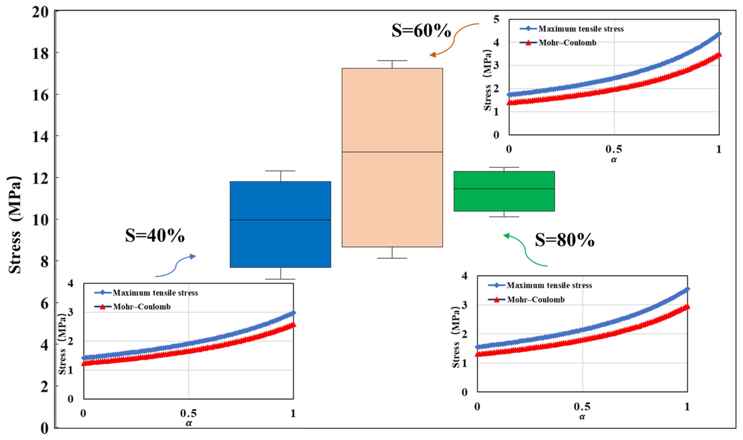
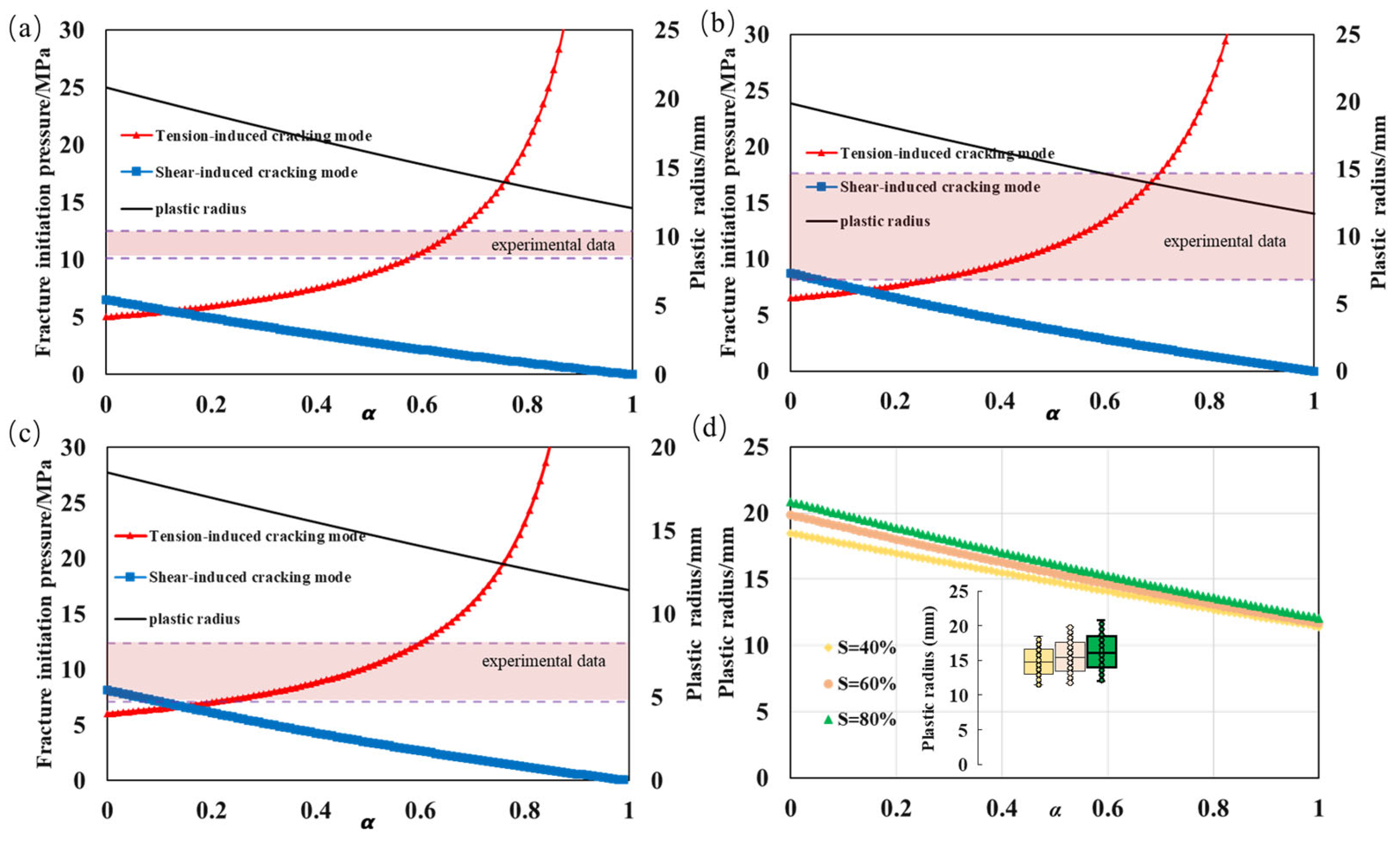
4.3. Exploration of the Mechanism of Fracture Initiation Pressure
4.3.1. Criterion for Rock Failure
- Maximum tensile stress criterion
- 2.
- Mohr–Coulomb criterion
4.3.2. Calculation of Fracture Initiation Pressure
- Tension-induced cracking mode
- 2.
- Shear-induced cracking mode
5. Conclusions
Author Contributions
Funding
Data Availability Statement
Conflicts of Interest
Appendix A
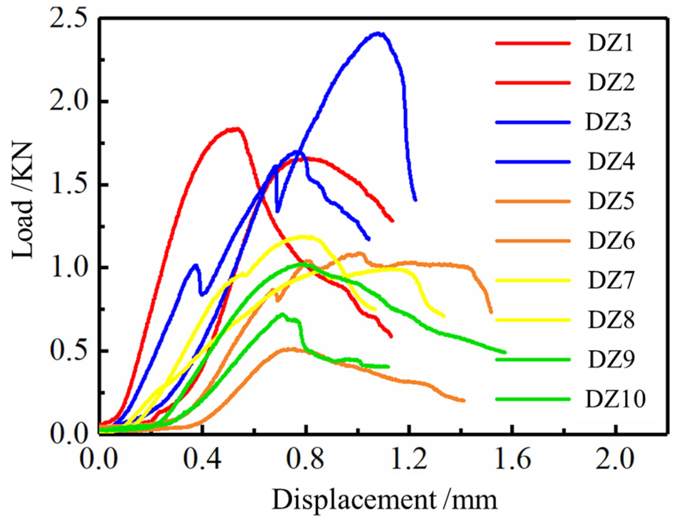
Appendix A.1

| Sample ID | Cement Content (%) | Water Addition (%) | Porosity (%) | Strength (MPa) |
|---|---|---|---|---|
| DZ1 | 18 | 35 | 35.14 | 3.84 |
| DZ2 | 18 | 35 | 35.72 | 3.45 |
| DZ3 | 18 | 30 | 23.14 | 5.01 |
| DZ4 | 18 | 30 | 34.25 | 3.49 |
| DZ5 | 16 | 35 | 36.45 | 1.44 |
| DZ6 | 16 | 35 | 35.77 | 1.98 |
| DZ7 | 16 | 33 | 38.58 | 2.07 |
| DZ8 | 16 | 33 | 37.33 | 2.47 |
| DZ9 | 16 | 30 | 35.92 | 1.59 |
| DZ10 | 16 | 30 | 34.04 | 2.1 |
Appendix A.2
Appendix A.3
Appendix A.4
References
- Boswell, R.; Shipp, C.; Reichel, T.; Shelander, D.; Saeki, T.; Frye, M.; Shedd, W.; Collett, T.S.; McConnell, D.R. Prospecting for marine gas hydrate resources. Interpretation 2016, 4, SA13–SA24. [Google Scholar] [CrossRef]
- Ren, X.; Guo, Z.; Ning, F.; Ma, S. Permeability of hydrate-bearing sediments. Earth-Sci. Rev. 2020, 202, 103100. [Google Scholar] [CrossRef]
- Kazakov, E.; Fayzullin, I.; Sheremeev, A.; Shurunov, A.; Chebykin, N.; Uchuev, R.; Serdyuk, A.; Vikhman, I.; Prunov, D. Unconventional approach for fracturing stimulation in conventional low-permeability formation by the example of experimental part South Priobskoe field. In Proceedings of the SPE Russian Petroleum Technology Conference, Moscow, Russia, 22–24 October 2019; p. D033S020R001. [Google Scholar]
- Li, Q.; Xing, H.; Liu, J.; Liu, X. A review on hydraulic fracturing of unconventional reservoir. Petroleum 2015, 1, 8–15. [Google Scholar] [CrossRef]
- Li, F.; Yuan, Q.; Li, T.; Li, Z.; Sun, C.; Chen, G. A review: Enhanced recovery of natural gas hydrate reservoirs. Chin. J. Chem. Eng. 2019, 27, 2062–2073. [Google Scholar] [CrossRef]
- Huang, M.; Wu, L.; Ning, F.; Wang, J.; Dou, X.; Zhang, L.; Liu, T.; Jiang, G. Research progress in natural gas hydrate reservoir stimulation. Nat. Gas Ind. B 2023, 10, 114–129. [Google Scholar] [CrossRef]
- Feng, Y.; Chen, L.; Suzuki, A.; Kogawa, T.; Okajima, J.; Komiya, A.; Maruyama, S. Enhancement of gas production from methane hydrate reservoirs by the combination of hydraulic fracturing and depressurization method. Energy Convers. Manag. 2019, 184, 194–204. [Google Scholar] [CrossRef]
- Sun, J.; Ning, F.; Liu, T.; Liu, C.; Chen, Q.; Li, Y.; Cao, X.; Mao, P.; Zhang, L.; Jiang, G. Gas production from a silty hydrate reservoir in the South China Sea using hydraulic fracturing: A numerical simulation. Energy Sci. Eng. 2019, 7, 1106–1122. [Google Scholar] [CrossRef]
- Khodaverdian, M.; McElfresh, P. Hydraulic fracturing stimulation in poorly consolidated sand: Mechanisms and consequences. In Proceedings of the SPE Annual Technical Conference and Exhibition, Dallas, TX, USA, 1–4 October 2000; p. SPE–63233. [Google Scholar]
- Ito, T.; Igarashi, A.; Suzuki, K.; Nagakubo, S.; Matsuzawa, M.; Yamamoto, K. Laboratory study of hydraulic fracturing behavior in unconsolidated sands for methane hydrate production. In Proceedings of the Offshore technology conference, Houston, TX, USA, 5–8 May 2008; p. OTC–19324. [Google Scholar]
- Konno, Y.; Jin, Y.; Yoneda, J.; Uchiumi, T.; Shinjou, K.; Nagao, J. Hydraulic fracturing in methane-hydrate-bearing sand. RSC Adv. 2016, 6, 73148–73155. [Google Scholar] [CrossRef]
- Lu, C.; Qin, X.; Mao, W.; Ma, C.; Geng, L.; Yu, L.; Bian, H.; Meng, F.; Qi, R. Experimental study on the propagation characteristics of hydraulic fracture in clayey-silt sediments. Geofluids 2021, 2021, 6698649. [Google Scholar] [CrossRef]
- Cao, Q.Y. Research on the Fracturability of Hydrate Reservoirs in Permafrost Regions. Master’s Thesis, China University of Petroleum (East China), Qingdao, China, 2017. [Google Scholar]
- Ma, X.; Jiang, D.; Sun, Y.; Li, S. Experimental study on hydraulic fracturing behavior of frozen clayey silt and hydrate-bearing clayey silt. Fuel 2022, 322, 124366. [Google Scholar] [CrossRef]
- Zhong, X.P. The Influence of Fracture Initiation-Propagation Behavior and Fracture Morphology on the Stimulation Potential of the Shenhu Hydrate Reservoir. Ph.D. Thesis, Jilin University, Changchun, China, 2022. [Google Scholar]
- Wang, X.; Sun, Y.; Chen, H.; Peng, S.; Jiang, S.; Ma, X. Experimental study on the depressurization of methane hydrate in the clayey silt sediments via hydraulic fracturing. Energy Fuels 2023, 37, 4377–4390. [Google Scholar] [CrossRef]
- Yu, Y.; Shen, K.; Zhao, H. Experimental Investigation of Fracture Propagation in Clayey Silt Hydrate-Bearing Sediments. Energies 2024, 17, 528. [Google Scholar] [CrossRef]
- Yao, Y.; Guo, Z.; Zeng, J.; Li, D.; Lu, J.; Liang, D.; Jiang, M. Discrete element analysis of hydraulic fracturing of methane hydrate-bearing sediments. Energy Fuels 2021, 35, 6644–6657. [Google Scholar] [CrossRef]
- Ma, X.; Cheng, J.; Sun, Y.; Li, S. 2D numerical simulation of hydraulic fracturing in hydrate-bearing sediments based on the cohesive element. Energy Fuels 2021, 35, 3825–3840. [Google Scholar] [CrossRef]
- Ju, X.; Liu, F.; Fu, P.; White, M.D.; Settgast, R.R.; Morris, J.P. Gas production from hot water circulation through hydraulic fractures in methane hydrate-bearing sediments: THC-coupled simulation of production mechanisms. Energy Fuels 2020, 34, 4448–4465. [Google Scholar] [CrossRef]
- Too, J.L.; Cheng, A.; Khoo, B.C.; Palmer, A.; Linga, P. Hydraulic fracturing in a penny-shaped crack. Part I: Methodology and testing of frozen sand. J. Nat. Gas Sci. Eng. 2018, 52, 609–618. [Google Scholar] [CrossRef]
- Singh, B.; Lal, B.; Manjusha, A. Gas hydrate in oil and gas systems. In Gas Hydrate in Carbon Capture, Transportation and Storage; CRC Press: Boca Raton, FL, USA, 2024; pp. 1–17. [Google Scholar]
- Liu, J.; Kong, L.; Zhao, Y.; Sang, S.; Niu, G.; Wang, X.; Zhou, C. Test research progress on mechanical and physical properties of hydrate-bearing sediments. Int. J. Hydrog. Energy 2024, 53, 562–581. [Google Scholar] [CrossRef]
- Sun, J.Y.; Li, C.F.; Hao, X.L.; Liu, C.L.; Chen, Q.; Wang, D.G. Study of the surface morphology of gas hydrate. J. Ocean. Univ. China 2020, 19, 331–338. [Google Scholar] [CrossRef]
- Xiao, G.; Bai, Y.H. Natural Gas Hydrates—Flammable Ice; Wuhan University Press: Wuhan, China, 2012. [Google Scholar]
- Luo, T.; Song, Y.; Zhu, Y.; Liu, W.; Liu, Y.; Li, Y.; Wu, Z. Triaxial experiments on the mechanical properties of hydrate-bearing marine sediments of South China Sea. Mar. Pet. Geol. 2016, 77, 507–514. [Google Scholar] [CrossRef]
- Yang, F.; Li, C.; Wei, N.; Jia, W.; He, J.; Song, S.; Zhang, Y.; Lin, Y. Mechanical properties and constitutive model of high-abundance methane hydrates containing clayey–silt sediments. Ocean. Eng. 2024, 298, 117245. [Google Scholar] [CrossRef]
- Jones, R.M. Deformation theory of plasticity. Bull Ridge Corporation: Blacksburg, Virginia, USA, 2009. [Google Scholar]
- Nie, S.S. Hydraulic Fracture Formation Mechanism and Multi-Layer Fracturing Co-Production Behavior of Oceanic Non-Diagenetic Natural Gas Hydrate Reservoir. Ph.D. Thesis, Jilin University, Changchun, China, 2023. [Google Scholar]
- Beer, F.P.; Johnston, E.R.; DeWolf, J.T.; Mazurek, D.F.; Sanghi, S. Mechanics of Materials; Mcgraw-Hill: New York, NY, USA, 1992. [Google Scholar]
- Lemaitre, J.; Chaboche, J.L. Mechanics of Solid Materials; Cambridge University Press: Cambridge, UK, 1994. [Google Scholar]
- Craig, R.R., Jr.; Taleff, E.M. Mechanics of Materials; John Wiley & Sons: Hoboken, NJ, USA, 2020. [Google Scholar]
- Xu, Y.B. Characteristics of Water Retention and Tensile Strength of Hydrate-Containing Soil. Guilin University of Technology, Guilin, China. 2023. Available online: https://kns.cnki.net/kcms2/article/abstract?v=X7jC3qydZ58vLF5RdtoXzzX-UxsPoR7x2GXaX8PZ4Gfgdom4PNZcKS-18Ho83819B-abZSo3nPjxsFnU1C6hnb5A86iLaRgjIgFs3keM_h_JqzaaQFXS1jAPhbHizdThQ-uutYAKrvojhQUTWwN4CMtgdHhpswNpZapJrcOhnWBHLoozsZEfhLGmJ1kdgUZ3&uniplatform=NZKPT&language=CHS (accessed on 21 April 2025).
- Miyazaki, K.; Sakamoto, Y.; Kakumoto, M.; Tenma, N.; Aoki, K.; Yamaguchi, T. Triaxial compressive properties of artificial methane-hydrate-bearing sediments containing fine fraction. J. MMIJ 2011, 127, 565–576. [Google Scholar] [CrossRef]
- Masui, A.; Haneda, H.; Ogata, Y.; Aoki, K. Mechanical properties of sandy sediment containing marine gas hydrates in deep sea offshore Japan. In Proceedings of the ISOPE Ocean Mining and Gas Hydrates Symposium, Lisbon, Portugal, 1–6 July 2007; p. ISOPE-M-07-015. [Google Scholar]
- Miyazaki, K.; Masui, A.; Tenma, N.; Ogata, Y.; Aoki, K.; Yamaguchi, T.; Sakamoto, Y. Study on mechanical behavior for methane hydrate sediment based on constant strain-rate test and unloading-reloading test under triaxial compression. Int. J. Offshore Polar Eng. 2010, 20, 61–67. [Google Scholar]
- Liu, Z.; Wei, H.; Peng, L.; Wei, C.; Ning, F. An easy and efficient way to evaluate mechanical properties of gas hydrate-bearing sediments: The direct shear test. J. Pet. Sci. Eng. 2017, 149, 56–64. [Google Scholar] [CrossRef]
- Shi, Y.H.; Zhang, X.H.; Lu, X.B.; Wang, S.Y.; Wang, A.L. Experimental Study on the static mechanical properties of hydrate-bearing silty-clay in the South China Sea. Chin. J. Theor. Appl. Mech. 2015, 47, 521–528. [Google Scholar]
- Masui, A.; Haneda, H.; Ogata, Y.; Aoki, K. The effect of saturation degree of methane hydrate on the shear strength of synthetic methane hydrate sediments. In Proceedings of the 5th International Conference on Gas Hydrates, Trondheim, Norway, 13–16 June 2005; pp. 657–663. [Google Scholar]


| Item | Ice | NGH I | NGH II |
|---|---|---|---|
| Lattice diameter (0 °C) | 4.52 | 11.97 | 17.14 |
| Volume expansion coefficient (k−1) | 1.5 × 10⁻⁴ | 1.5 × 10⁻⁴ | 1.7 × 10⁻⁴ |
| Isothermal Young’s modulus at −5 °C (109 Pa) | 9.5 | 8.4 | 8.2 |
| Poisson’s ratio | 0.33 | 0.33 | 0.33 |
| Adiabatic bulk modulus at 0 °C (Pa) | 12 × 10−11 | 14 × 10−11 | 14 × 10−11 |
| Longitudinal sound velocity (km·s−1) | 4 | 3.8 | 3.8 |
| The enthalpy of formation of a crystal lattice compared to gas at 0 °C (kJ·mol−1) | −51.01 | −50.2 | −50.2 |
| Lattice energy at 0 K (kJ·mol−1) | −47.3 | Slightly lower than ice | Slightly lower than ice |
| Residual entropy at 0 K (J·kmol−1) | 3.43 | Slightly lower than ice | Slightly lower than ice |
| Density at 0 °C (g·cm−3) | 0.912 | 0.91 | 0.883 |
| Group Number | Sample ID | (MPa) | Injection Rate (L·min−1) | Viscosity (mPa·s) | Ice Saturation (%) | Perforation Patterns |
|---|---|---|---|---|---|---|
| A1 | 1# | 3/1.5/1.5 | 14 | 1 | 0 | 180-degree directional hole layout |
| 2# | 20 | |||||
| 3# | 40 | |||||
| 4# | 60 | |||||
| 5# | 80 | |||||
| A2 | 6# | 3/1.5/1.5 | 14 | 5 | 0 | 180-degree directional hole layout |
| 7# | 20 | |||||
| 8# | 40 | |||||
| 9# | 60 | |||||
| 10# | 80 | |||||
| A3 | 11# | 3/1.5/1.5 | 10 | 30 | 0 | 180-degree directional hole layout |
| 12# | 20 | |||||
| 13# | 40 | |||||
| 14# | 60 | |||||
| 15# | 80 | |||||
| A4 | 16# | 3/1.5/1.5 | 8 | 60 | 0 | 180-degree directional hole layout |
| 17# | 20 | |||||
| 18# | 40 | |||||
| 19# | 60 | |||||
| 20# | 80 | |||||
| A5 | 21# | 3/1.5/1.5 | 6 | 80 | 0 | 180-degree directional hole layout |
| 22# | 20 | |||||
| 23# | 40 | |||||
| 24# | 60 | |||||
| 25# | 80 | |||||
| B | 26# | 3/1.5/1.5 | 5 | 1 | 40 | 180-degree directional hole layout |
| 27# | 6 | |||||
| 28# | 8 | |||||
| C | 29# | 4/2/1 | 14 | 1 | 40 | 180-degree directional hole |
| 30# | 5/3/1 | |||||
| 31# | 5/3/1.5 | |||||
| D | 32# | 3/1.5/1.5 | 14 | 1 | 40 | 60-degree helical hole layout |
| 33# | 90-degree helical hole layout | |||||
| 34# | 180-degree directional hole layout | |||||
| 35# | 90-degree fixed-plane hole layout | |||||
| 36# | open-hole perforation-free pipe |
| Saturation S, % | 40 | 60 | 80 |
|---|---|---|---|
| , MPa | 0.323 | 0.319 | 0.235 |
| , % | 0.47 | 0.32 | 0.62 |
| , MPa | 2.3640 | 2.7154 | 2.2504 |
| , % | 3.578 | 3.828 | 6.090 |
| elastic modulus , MPa | 72.266 | 109.840 | 35.236 |
| yield coefficient | 0.72 | 0.77 | 0.68 |
| softening coefficient | 0.97 | 0.95 | 1.09 |
| Serial No. | |||||
|---|---|---|---|---|---|
| 1 | [0.65, 0.80] | 0.5 | 0.3 | 4.9 | 2.50 |
| 2 | 0.70 | [0.3, 0.7] | 0.3 | 4.9 | 2.50 |
| 3 | 0.70 | 0.5 | [0.2, 0.4] | 4.9 | 2.50 |
| 4 | 0.70 | 0.5 | 0.3 | [3.6, 6.2] | 2.50 |
| 5 | 0.70 | 0.5 | 0.3 | 4.9 | [2.25, 2.75] |
| Parameter | Value | Parameter | Value |
|---|---|---|---|
| (MPa) | 3, 1.5, 1.5 | well deviation angle (°) | 90 |
| azimuth angle (°) | 90 | wellbore circumference angle (°) | 0 |
| (mm) | 150 | (MPa) | 0.1 |
| (mm) | 7.5 | 0.25 | |
| cohesive strength (MPa) | internal friction angle (°) | 33 | |
| , MPa | along with the selected constitutive model |
Disclaimer/Publisher’s Note: The statements, opinions and data contained in all publications are solely those of the individual author(s) and contributor(s) and not of MDPI and/or the editor(s). MDPI and/or the editor(s) disclaim responsibility for any injury to people or property resulting from any ideas, methods, instructions or products referred to in the content. |
© 2025 by the authors. Licensee MDPI, Basel, Switzerland. This article is an open access article distributed under the terms and conditions of the Creative Commons Attribution (CC BY) license (https://creativecommons.org/licenses/by/4.0/).
Share and Cite
Shen, K.; Yu, Y.; Zhang, H.; Xie, W.; Lu, J.; Zhou, J.; Wang, X.; Wang, Z. Triaxial Experimental Study of Natural Gas Hydrate Sediment Fracturing and Its Initiation Mechanisms: A Simulation Using Large-Scale Ice-Saturated Synthetic Cubic Models. J. Mar. Sci. Eng. 2025, 13, 1065. https://doi.org/10.3390/jmse13061065
Shen K, Yu Y, Zhang H, Xie W, Lu J, Zhou J, Wang X, Wang Z. Triaxial Experimental Study of Natural Gas Hydrate Sediment Fracturing and Its Initiation Mechanisms: A Simulation Using Large-Scale Ice-Saturated Synthetic Cubic Models. Journal of Marine Science and Engineering. 2025; 13(6):1065. https://doi.org/10.3390/jmse13061065
Chicago/Turabian StyleShen, Kaixiang, Yanjiang Yu, Hao Zhang, Wenwei Xie, Jingan Lu, Jiawei Zhou, Xiaokang Wang, and Zizhen Wang. 2025. "Triaxial Experimental Study of Natural Gas Hydrate Sediment Fracturing and Its Initiation Mechanisms: A Simulation Using Large-Scale Ice-Saturated Synthetic Cubic Models" Journal of Marine Science and Engineering 13, no. 6: 1065. https://doi.org/10.3390/jmse13061065
APA StyleShen, K., Yu, Y., Zhang, H., Xie, W., Lu, J., Zhou, J., Wang, X., & Wang, Z. (2025). Triaxial Experimental Study of Natural Gas Hydrate Sediment Fracturing and Its Initiation Mechanisms: A Simulation Using Large-Scale Ice-Saturated Synthetic Cubic Models. Journal of Marine Science and Engineering, 13(6), 1065. https://doi.org/10.3390/jmse13061065