Abstract
Ria de Arousa, one of the Rias Baixas, presents very high economic value for the Galician communities due to its importance for aquaculture, but the changes associated with climate change are expected to have an impact on its hydrodynamics and consequently on the production of cultivated species. The main objective of this work is to study the impact of climate change on the circulation and hydrography of the Ria de Arousa, considering the SSP5-8.5 scenario defined by IPCC. To achieve this goal, the Delft3D hydrodynamic model was implemented three-dimensionally using the results obtained from the CMIP6 MPI-ESM1-2-HR climate model as boundary conditions. Future changes in the hydrodynamic and hydrographic circulation of this coastal system were analysed. The model results were used to assess the impact of climate change on water temperature, salinity, and density patterns of the Ria de Arousa, as well as on stratification, Brunt–Väisälä frequency, and residual circulation. During summer, the water temperature is higher at the surface and lower at the bottom, likely due to the intrusion of water from the Eastern North Atlantic Central Water (ENAWC). In the future, this pattern will continue, albeit with higher temperatures, as the water temperature is expected to increase by around 2.2 °C by 2100. During winter, the water temperature at the bottom is warmer than at the surface, indicating a thermal inversion typical of this season. In the future, the water temperature will also increase, although the increase will be lower compared to summer, with a value of approximately 0.5 °C. Salinity will decrease in the summer and increase in the winter, especially in the areas closest to the rivers. Density analysis shows vertical homogeneity in the water column during winter and stratification during summer. During winter, the Brunt–Väisälä frequency (N) is higher in the region closest to the river’s mouth and lower near the ocean. In the summer, the N value decreases with depth. In the future, the density will increase in winter and decrease in summer, and stratification is expected to decrease. Regarding the residual circulation, it was observed that it will strengthen in the summer and weaken in the winter due to a decrease in freshwater runoff. However, the positive circulation pattern observed in the present will be maintained in the future.
1. Introduction
Oceans and coastal ecosystems host vast biodiversity that plays a pivotal role in regulating global climate systems by managing heat, water, and other essential elements, such as carbon. These marine environments hold great cultural significance in many societies and serve as sources of sustenance, minerals, energy, and employment for many people. In marine systems, changes in hydrodynamical patterns pose a significant threat to low-lying coastal areas that often present high economic and biological value. The Rias Baixas (Figure 1a), constituted by the Ria de Vigo, the Ria de Pontevedra, the Ria de Arousa, and the Ria de Muros, are located in Galicia (NW Spain), where local communities strongly depend on the income brought by aquaculture [1]. They comprise the largest production area in Spain, with more than 90% of all mussel (Mytilus spp.) production, comprising 3266 mussel rafts, 69% of which are located in Ria de Arousa [2]. This sector directly generates over 8000 jobs, and its annual output represents approximately 50% of global mussel production, placing Spain among the top global aquaculture producers [3]. Therefore, understanding how climate change will affect the Rias Baixas hydrodynamics is essential to foresee the expected impact on local aquaculture activities.
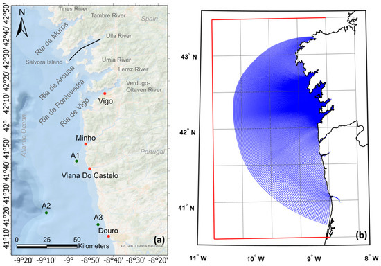
Figure 1.
(a) Map of the Rias Baixas showing the longitudinal section (black line), tidal stations (red dots), and sampling locations for salinity and water temperature (green dots). (b) Delft3D numerical grid (blue), showing the climate model grid (grey) and its corresponding boundary (red line).
The Ria de Arousa, considered an estuarine system, is located between 42°27′ N and 42°41′ N and 8°44′ W and 9°01′ W, and it is the most extensive of the Rias Baixas [4]. It has a surface area of 230 km2, a volume of 4.5 × 10⁹ m3, and a mean depth of 19 m, reaching a maximum of 70 m in the southern mouth. It has a V-shaped configuration, progressively widening from the innermost part to the mouth [3]. The connection with the ocean is marked by Salvora Island, which divides the mouth of the Ria in two: the northern mouth, approximately 10 m depth, is shallower than the southern mouth, which is 70 m deep, and is where most of the exchanges with the shelf occur [5]. The tidal range observed in this Ria ranges between 1.5 and 3.7 m [5], and the main freshwater inputs are the rivers Ulla and Umia, with an average flow rate of 93 m3/s and 16 m3/s, respectively [6]. The Ria de Arousa behaves as a partially mixed estuary with positive residual circulation, maintained by the river discharge in the winter and by solar heating in the summer [7]. This circulation is intensified by coastal upwelling in the summer, which introduces the colder and nutrient-rich Eastern North Atlantic Central Water (ENACW) into the system [7]. The water mass along the Ria de Arousa is a mixture of coastal seawater and freshwater coming from the rivers discharging in this system. Thus, its properties depend on the characteristics of the ocean and fluvial drivers and their mixing ratio [6].
In the Ria de Arousa, there is an asymmetry between the upwelling and downwelling conditions, as concluded by [8]. During upwelling events, the Ria becomes stratified with through-flow crossing directly between the islands. The inflow occurs along the bottom through both mouths, while surface outflow takes place exclusively through the southern mouth. Under these conditions, the river outflow is flushed out, and the Ria is quickly filled with upwelled ENACW. In contrast, during downwelling, this estuarine system tends to be homogenous. The through-flow is circuitous, the outflow occurs through both mouths, and the inflow is restricted to a thick surface layer (~15 m) that enters the Ria exclusively via the southern mouth. Several works have been developed to study the circulation and physical properties of the Ria de Arousa, starting in 1975 when [9] performed a hydrographic analysis in this area. After that, ref. [5] studied the variation in thermohaline and chemical properties and found that the variability in physical and chemical parameters in the surface layer is primarily driven by atmospheric and continental influences, while the variations in the deep layer are governed by the upwelling and downwelling dynamics.
The aforementioned studies focused on characterising the behaviour and patterns observed in the Ria de Arousa based on historical data. In recent years, studies have also focused on the effect of climate change on these estuaries. Refs. [1,10] studied, using CMIP5 data, how climate change, namely, changes in water temperature and stratification, will affect the Rias Baixas and its effect on mussel aquaculture productivity. Also utilising CMIP5 data, ref. [10] modelled the salinity drop in estuarine areas under extreme precipitation events within the context of climate change and the effect it may have on bivalve mortality in the Rias Baixas.
To date, no studies have specifically employed climate projections from the Coupled Model Intercomparison Project Phase 6 (CMIP6) to assess the potential impacts of climate change on the Ria de Arousa.
CMIP6 is Phase 6 of the Coupled Model Intercomparison Project, and it informs much of the physical science basis for the Sixth Assessment Report (AR6) of the Intergovernmental Panel on Climate Change (IPCC). It features the latest generation of comprehensive Earth system models (ESMs), which are driven by historical greenhouse gas (GHG) concentrations and followed by different future greenhouse gas and aerosol concentrations based on Shared Socioeconomic Pathways (SSP) scenarios [11]. These incorporate a range of assumptions, including socioeconomic trends and mitigation options. The very low and low GHG emission scenarios are SSP1-1.9 and SSP1-2.6, which have CO2 emissions declining to net zero around 2050 and 2070, respectively, followed by varying levels of net-negative CO2 emissions. The intermediate scenario is SSP2-4.5, where CO2 emissions remain around current levels until the middle of the century. And finally, in the high and very high GHG emission scenarios, SSP3-7.0 and SSP5-8.5, CO2 emissions roughly double from current levels by 2100 and 2050, respectively [12].
This research aims to address this knowledge gap by integrating the most pessimistic CMIP6 scenario, SSP5-8.5, into a numerical modelling framework to explore future changes in the circulation and hydrography of this estuarine system. The findings provide critical insights into the potential effects of climate change on the Ria de Arousa, supporting the development of science-based strategies for its sustainable management and adaptation. Accordingly, the main objective of this study is to evaluate the impact of climate change on the hydrodynamics of the Ria de Arousa. To achieve this, a three-dimensional baroclinic model, encompassing all the Rias Baixas and the adjacent coastal region to simulate all their interactions, was implemented using variables derived from global and regional climate models under future CMIP6 scenarios.
2. Materials and Methods
2.1. Delft3D Numerical Model Implementation
The numerical model used in this study was Delft3D. The Delft3D-Flow module has been implemented successfully in several coastal and estuarine studies [13,14,15,16,17], and it has even been applied in the Rias Baixas, both individually and in all the Rias Baixas together. For example, ref. [18] applied this model in the Ria de Vigo, several authors [19,20,21,22] implemented it in the Ria de Muros, and [10,23] successfully implemented the Delft3D model in all the Rias Baixas.
2.1.1. Grid and Bathymetry
A numerical grid was constructed, expanded, and orthogonalised based on previous work developed by the University of Aveiro’s Estuarine and Coastal Modelling Group as part of the SMART Project, which previously validated this implementation. A numerical model was designed using a curvilinear grid with fine resolution in the Rias Baixas (190 m) coarsening towards the ocean (1600 m) and 26 sigma layers with higher discretisation at the surface layers. This grid covers an area from 40.8° N to 43.3° N and from 8.6° W to 10.5° W, creating a total number of grid cells of 224 × 362 (Figure 1b). It includes all four Rias Baixas and the adjacent coastal area, as well as the Minho, Lima, and Douro outflows because, as mentioned previously, the estuarine plumes can affect the circulation in some of the Rias [18,23,24].
The bathymetry was obtained from the General Bathymetric Chart of the Oceans (GEBCO). This grid is a global terrain model for ocean and land, and it provides global coverage of elevation data, in meters, on a 15-arcsecond interval grid.
2.1.2. Reference Implementation and Validation
Thirty-four tidal harmonic constituents obtained from the FES2014 global ocean tide atlas, which is the latest version of the FES (Finite Element Solution) tide model with a spatial resolution of about 7 km, were prescribed as astronomical forcing at the open ocean boundary. The open ocean boundary conditions for water temperature and salinity were retrieved from the operational Atlantic-Iberian Biscay Irish-Ocean Physics Reanalysis product provided by the Copernicus Marine Environment Monitoring Service (CMEMS), with a horizontal resolution of 1/12° and a vertical resolution of 50 sigma layers. The surface boundary conditions were defined considering hourly meteorological data from MeteoGalicia (the regional meteorological agency) obtained as means from the Weather Research and Forecasting Model with a resolution of 12 km. Freshwater discharges, also obtained from MeteoGalicia, were imposed as fluvial open boundary conditions.
The tidal wave propagation and the salt and heat transport processes were validated by comparing the model results with in situ data from four tide gauges (Douro, Viana do Castelo, Minho, and Vigo) and three Acoustic Doppler Current Profilers (ADCP) (A1, A2, and A3) (Figure 1a). To quantify the model reproducing in situ data, statistical analysis of the different stations was performed using Root Mean Square Error (RMSE), Bias, and Skill:
where Mod corresponds to the model and Obs corresponds to the observed values. RMSE provides a single number summarising the overall magnitude of the errors in a model’s predictions. It includes both systematic and random errors. Bias indicates the systematic error of a model, revealing its tendency to consistently over- or underestimate the observed values. Additionally, the Skill metric ranges from 0 to 1, where 1 indicates perfect agreement between model results and observations, and 0 indicates no agreement.
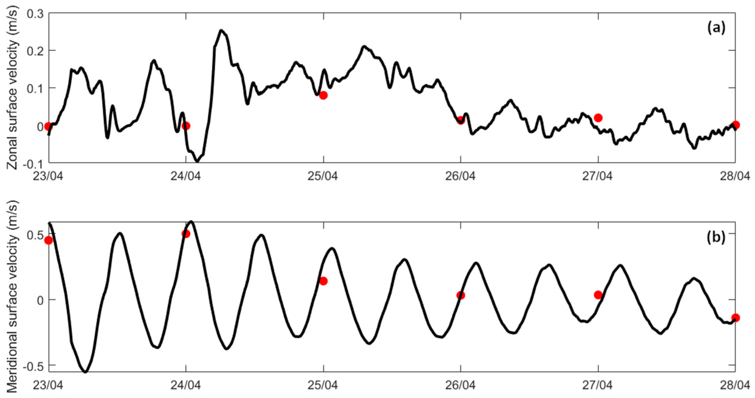
The zonal and meridional components of the surface current velocities were analysed for the A1 sampling station, and the findings are represented in Figure 2. Comparing the results of the ADCP measurements and the model output, it is possible to see that for both the zonal (Figure 2a) and meridional (Figure 2b) surface velocities, values align closely across the entire period. Two minor discrepancies were noted, on 25 and 27 of April, where slight deviations between the modelled and observed values occurred. However, these differences are within an acceptable range and do not significantly detract from the model’s overall performance.
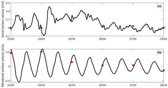
Figure 2.
Observed (red) and modelled (black) zonal (a) and meridional (b) components of the surface current velocities in sampling station A1.
In general, for all the stations, a good agreement between predicted tidal data and model results was achieved. The Minho tidal station shows the best results, with an RMSE of 0.058 m and a Skill of 0.999. The Douro tidal station also shows a Skill of 0.999 but an RMSE of 0.062 m. The highest RMSE is found at the Viana do Castelo tidal station with a value of 0.096 m, and both this station and the Vigo tidal station show a Skill of 0.996.
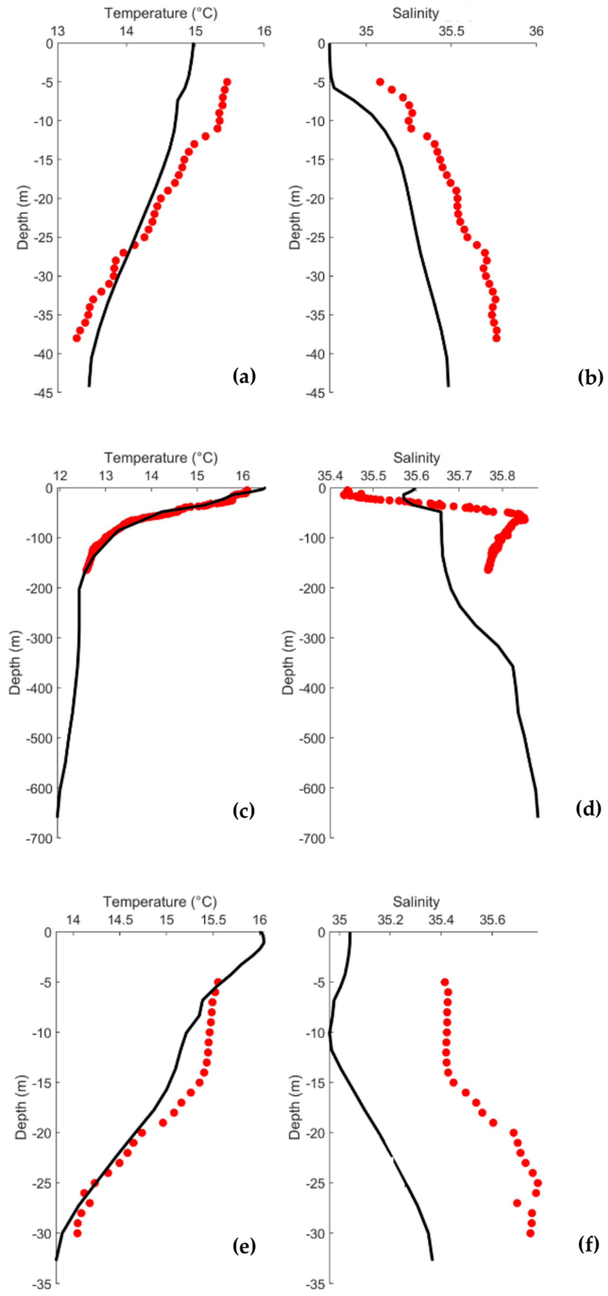
The water temperature and salinity profiles for each station are represented in Figure 3. The water temperature profiles show the same pattern between observed and modelled water temperatures (Figure 3a,c,e), showing small differences (<0.5 °C), with higher values at the surface and decreasing towards greater depths. Salinity profiles (Figure 3b,d,f) show a consistent pattern, with minor variations in the deeper regions further from the shore. The differences in salinity are small, less than 0.3. In general, a good fit was found between model predictions and observations, revealing the model’s ability to reproduce the in situ conditions accurately. These can be corroborated by the RMSE, Skill, and Bias determined for each station. For the salinity and water temperature, the RMSE, Bias, and Skill were calculated. Regarding water temperature, Station A1 showed the worst performance in all the parameters with an RMSE of 0.344 °C, a Skill of 0.906, and a Bias of 0.161 °C. Station A2 showed the best agreement with an RMSE of 0.131 °C, a Skill of 0.997, and a Bias of −0.027 °C. As for salinity, Station A3 performed the worst, showing the highest RMSE (0.458) and the highest Bias (0.457); however, it showed the highest Skill (0.813). Station A2 showed the lowest RMSE (0.131) and the lowest Bias (0.095), and the Skill was 0.464. Station A1 showed an RMSE of 0.298, a Skill of 0.609, and a Bias of 0.094.
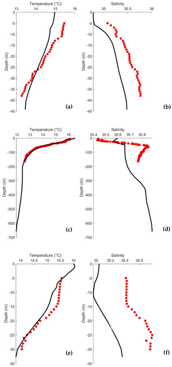
Figure 3.
Observed (red) and modelled (black) water temperature and salinity profiles for stations A1 (a,b), A2 (c,d), and A3 (e,f).
2.1.3. Climate Scenarios
After validating the reference configuration, the climate scenarios were simulated to achieve the goals of this study.
- i.
- Open ocean boundary.
Considering the reference implementation, for the future scenario, an increase in mean sea level of 0.7 m was applied. This value is based on the IPCC WGI Interactive Atlas, where the most pessimistic SSP5-8.5 scenario for the long-term period (2081–2100) was considered.
Transport conditions (salinity and water temperature) were also imposed at the open boundary based on a climatological mean from 1995 to 2014 of daily results from the Iberian–Biscay–Ireland (IBI) ocean reanalysis product. For the future SSP5-8.5 scenario simulations, a trend of the water temperature and salinity was calculated based on monthly data ranging from 2015 to 2099 from the MPI-ESM1-2-HR model (Figure 1b). This trend was then added to the data from the IBI used in the present scenario simulation. The selection of the MPI-ESM1-2-HR model was based on previous studies that provide a comparison with the other CMIP6 models available. Ref. [25] evaluated the performance of all CMIP6 models in simulating sea surface temperature (SST) and sea surface salinity (SSS), and the results rank the MPI-ESM1-2-HR model as number 5 out of the 48 CMIP6 models analysed. Furthermore, ref. [26] MPI-ESM1-2-HR performs above average across all metrics considered, making it one of the better-performing CMIP6 models regarding salinity. The choice of this model for the study area is even further corroborated by [27], which selected this model as the best model for representing the water temperature and salinity along the continental northwestern Iberian coast.
- ii.
- Atmospheric open boundary.
Since the MPI-ESM1-2-HR model has the best performance in representing the water temperature and salinity along the northwestern Iberian coast, the results of this model were also used for the atmospheric open boundary. A statistical analysis of each atmospheric variable was conducted to assess if the MPI-ESM1-2-HR accurately reproduces past climatic conditions. This analysis compares a monthly mean of the dataset obtained from ERA5 with the MPI-ESM1-2-HR hindcasts over a historical period from 1998 to 2014.
Based on [27,28], the Root Mean Square Error (RMSE), Bias, and correlation coefficient (R) were used to calculate a score (SR) for each property to rank the climate model’s capability. The SR metric aims to evaluate the overall performance of a model by considering its inaccuracy (through RMSE), its Bias (through the absolute value of the Bias, ∣Bias∣), and the correlation between predictions and observations (R). It includes two important but different aspects of the error: the total error magnitude and the magnitude of the systematic error, and is calculated as follows:
The lower the score, the better the agreement between the model results and the observed data.
Regarding the score, the model best represents air temperature and radiation, while the wind speed performed worse with an overall higher score. However, discrepancies in wind speed are a common characteristic of climate models. Previous studies have shown that CMIP6 models generally fail in reproducing observations of near-surface wind speed at a global or regional scale [29,30].
Given this, MPI-ESM1-2-HR daily data were used as atmospheric conditions in the simulations. This model is represented on a regular Gaussian grid in the horizontal and 95 vertical levels, with a horizontal resolution of 100 km [31]. A climatology ranging from 1990 to 2014 for the historical simulations and from 2015 to 2099 for the future scenario was used.
- iii.
- Fluvial open boundaries.
River discharges for the major tributaries in the Rias Baixas were imposed as fluvial open boundary conditions in each estuary. The rivers considered were Douro, Lima, Minho, Oitavén-Verdugo (which discharges into the Ria de Vigo), Lerez (which discharges into the Ria de Pontevedra), Umia and Ulla (which discharge into the Ria de Arousa), and Tambre (which discharges into the Ria de Muros). For the historical period, a climatological daily mean (1981–2010) was calculated [32] using data from MeteoGalicia. For the future scenario, the most pessimistic conditions were considered, with a reduction of 25% in river discharges [33,34], which was applied to the historical climatological mean obtained previously.
- iv.
- Parameters and specifications.
The roughness formula used for bottom roughness was the Manning coefficient. Several values of the Manning coefficient were evaluated and, taking into account previous studies [18,34], a value of 0.024 was selected based on the predominant bathymetric features, which best reproduced the observed tidal wave amplitude, considering that an increase in the bottom friction will produce a decrease in the tidal wave amplitude. A time step of 30 s was applied. The background horizontal eddy viscosity and diffusivity were set to 10 m2/s and the background vertical eddy viscosity and diffusivity to 10 and 5 m2/s, respectively. A heat flux model was applied, where relative humidity (%), air temperature (°C), and the combined net (short-wave) solar and net (long-wave) atmospheric radiation (J/m2/s) were provided with data from the MPI-ESM1-2-HR model. The wind process considers speed (m/s) and direction (°); both variables were also provided from the MPI-ESM1-2-HR model. An overview of the final modelling configurations is presented in Table 1.

Table 1.
Parameters and specifications of model implementation.
2.2. Data Analysis
To characterise the thermohaline properties of the Ria de Arousa, the water temperature, salinity, and density were analysed. This analysis consisted of 13 h means during the spring tide tidal cycle for the summer and winter seasons. Spring tides correspond to periods of greater tidal range, which generally translates into more intense currents and greater vertical mixing. These processes are key to understanding the physical dynamics of the system and their influence on the distribution of water masses. Although spring tides are not always extreme, they significantly modulate nutrient transport and mixing, especially in transitional periods such as spring. Thus, they can play an important role in biological productivity, including the onset of phytoplankton blooms. The results are represented in the form of surface maps and a longitudinal section shown in (Figure 1a).
If a mass of water is moved up or down adiabatically (no exchange of heat or salt) over a short distance and then returns to its original position, the water column is considered stable [35]. To analyse the stability of the water column, the Brunt–Väisälä frequency (N) was calculated as follows [36]:
where g is the gravitational acceleration, ρ is the density, and z is the depth measured from the surface. Lower N values indicate that the water column is less stratified, and higher N values indicate the opposite. This variable was calculated for the spring tide tidal cycle during the summer and winter seasons, the most extreme scenarios. It is represented in the form of longitudinal sections.
Residual circulation in estuaries is driven by various physical mechanisms, specifically river discharge, along-estuary density gradient, nonlinear advection, asymmetric tidal mixing, and wind. Positively buoyant material is generally transported seaward, while negatively buoyant material tends to move landward [37]. Previous studies [22,38,39] have analysed the residual circulation in the Rias Baixas, but none have assessed how this phenomenon will be affected by climate change. To achieve that goal, the residual circulation was assessed by averaging the simulated velocity for each element of the model grid for 29.56 days, two times the MSF constituent period, which represents the variation of the water level in a spring/neap tide cycle and results from the interaction between the M2 and S2 constituents. This analysis was performed for the present scenario as a characterisation of the residual circulation in the study area and for the future scenario to determine the possible effects of climate change on the observed circulation patterns.
3. Results
3.1. Thermohaline Properties
Water temperature, salinity, and density are analysed in the form of surface maps and longitudinal sections for the mean of the spring tide values during the summer and winter seasons for the present, future, and differences between the two. Furthermore, an analysis of longitudinal sections of the N are also presented for spring tide during the summer and winter seasons in the present, in the future, and highlighting the differences that exist in these scenarios.
For this analysis, it is important to note that the scales on the figures were chosen to best represent the results and may differ across scenarios.
3.1.1. Summer’s Spring Tide
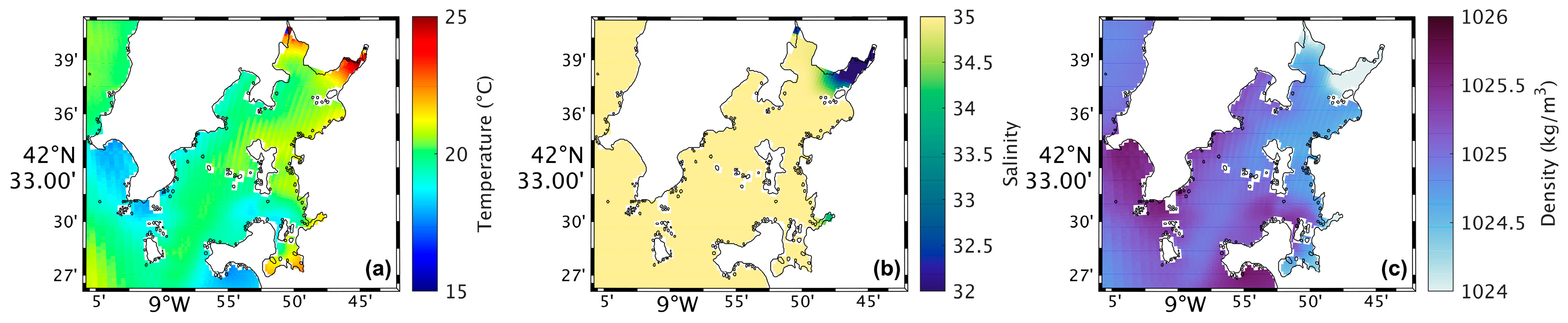
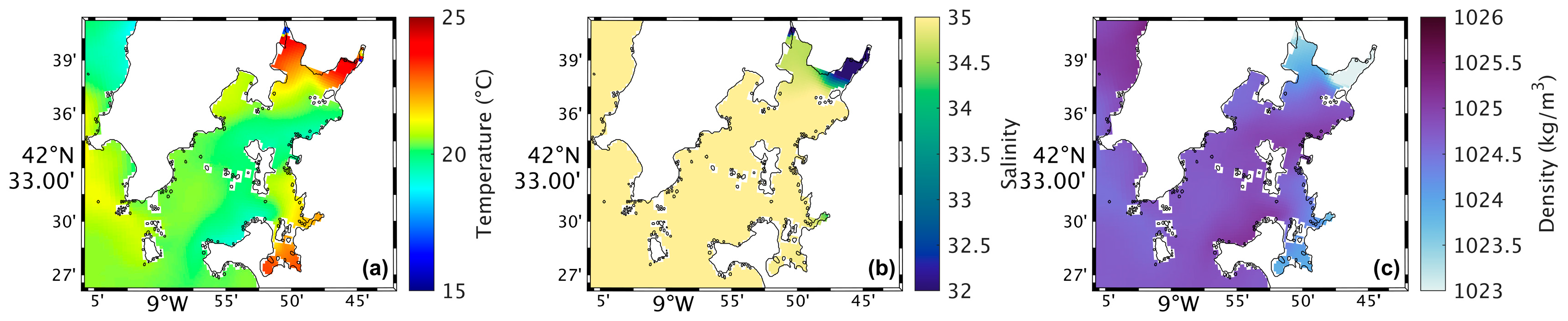
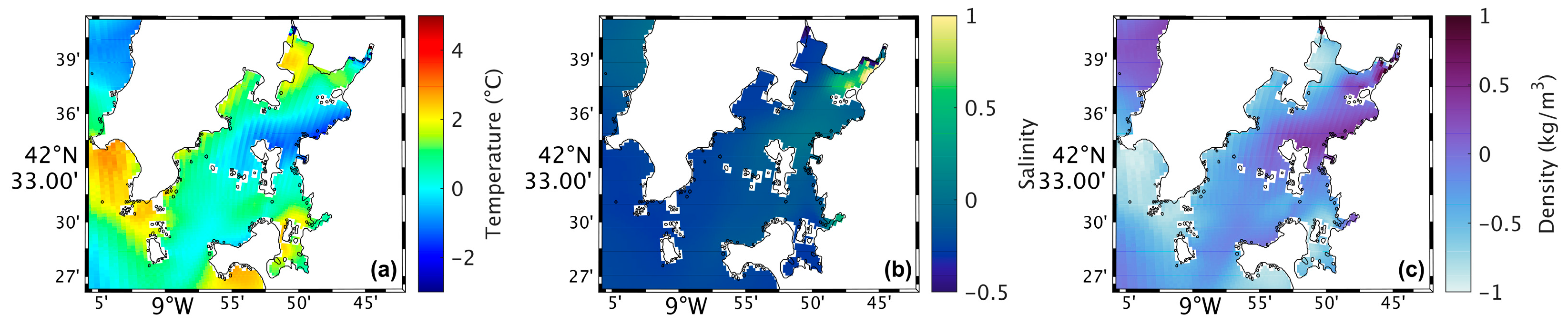
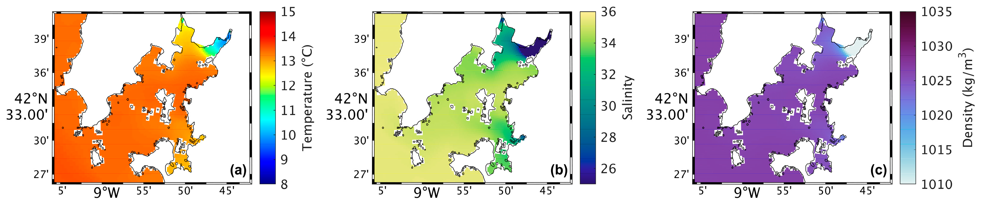
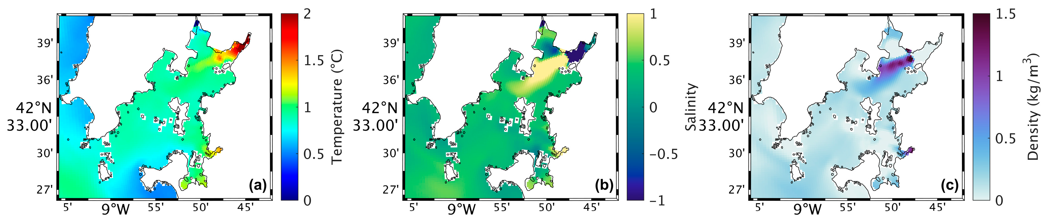
Figure 4a shows a map of the surface water temperature in the Ria de Arousa for the present scenario during summer spring tide. The highest water temperatures (around 25 °C) occur near the river’s mouth, while in the rest of the Ria, the temperatures range between 19 °C and 21 °C. In addition, the temperature decreases moving closer to the Ria’s connection with the ocean. In the future (Figure 5a), model results shows higher water temperatures near the river’s mouth and in the area near Arousa Island, making the changes (Figure 6a) 1.5 °C to 2 °C near the river’s mouth and −1.5 °C northeast of Arousa Island. The rest of the Ria shows increases of 1 °C and areas where there will be no change.

Figure 4.
Map of surface water temperature (a), salinity (b), and density (c) in the present during summer’s spring tide in the Ria de Arousa.

Figure 5.
Map of surface water temperature (a), salinity (b), and density (c) in the future during summer’s spring tide in the Ria de Arousa.

Figure 6.
Map of the differences between future and present in surface water temperature (a), salinity (b), and density (c) during summer’s spring tide in the Ria de Arousa.
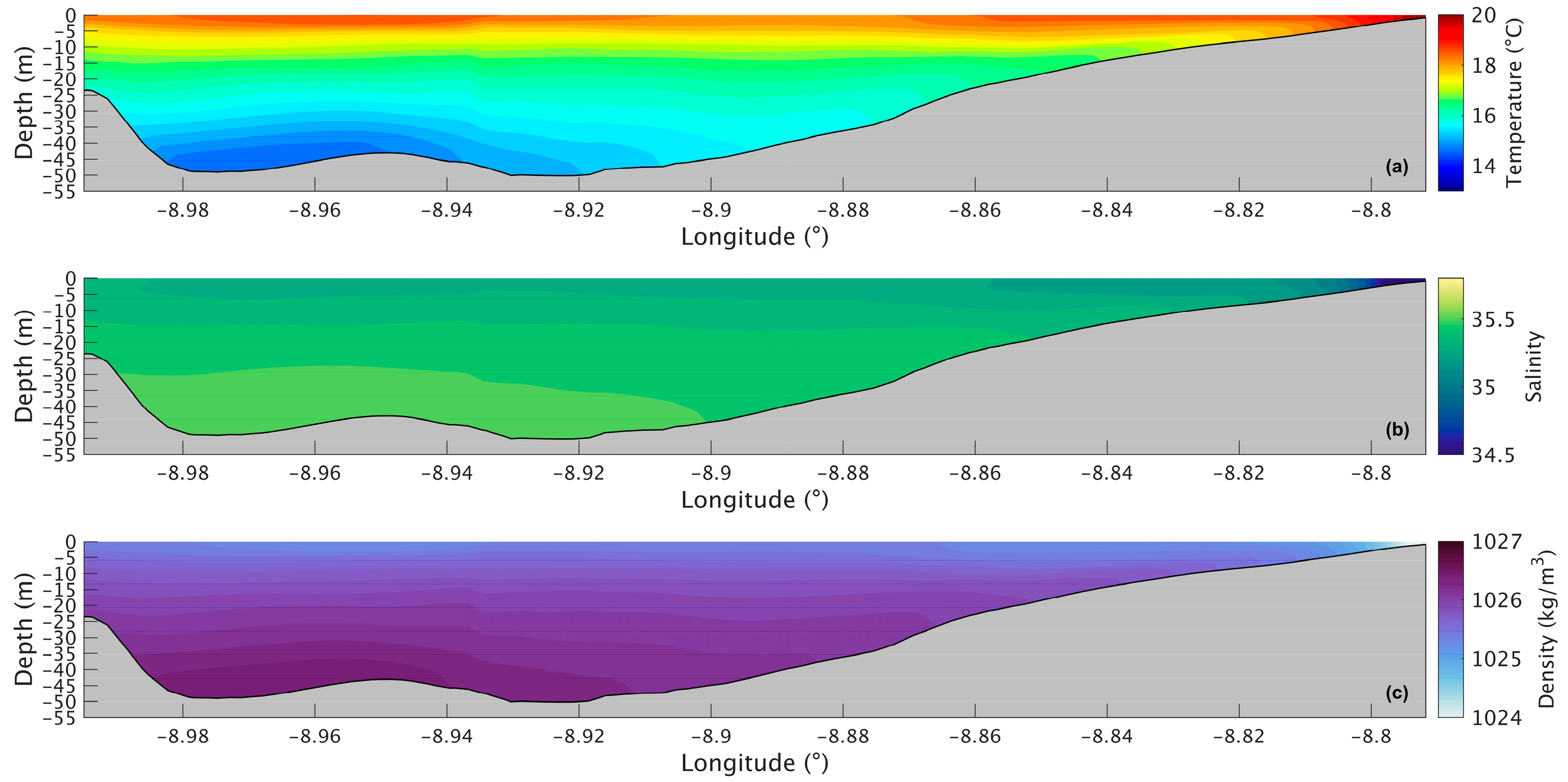
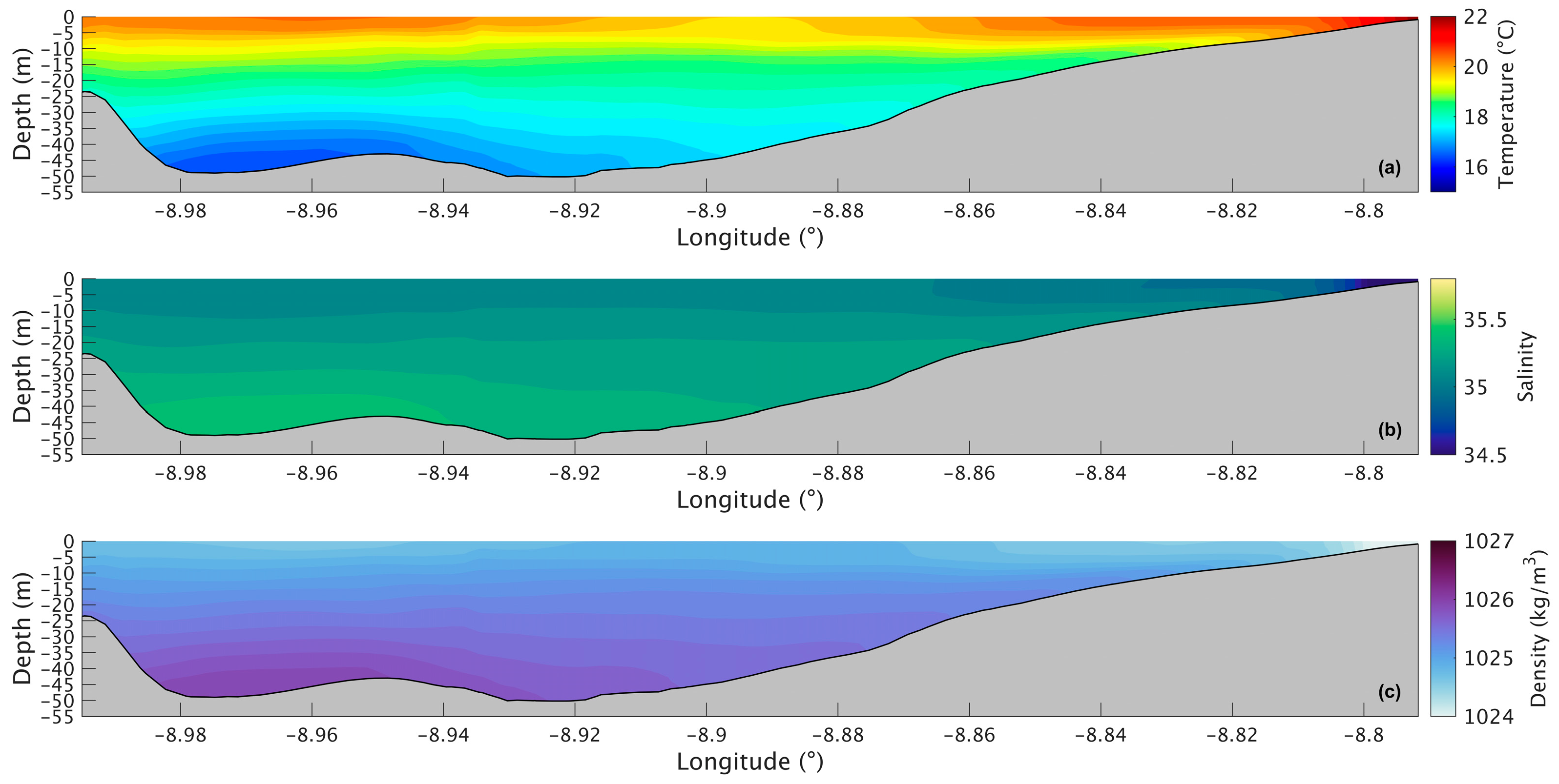
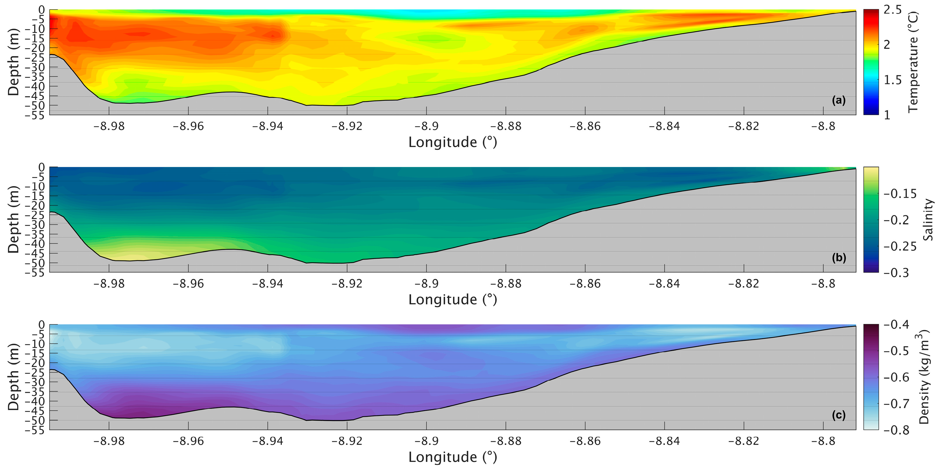
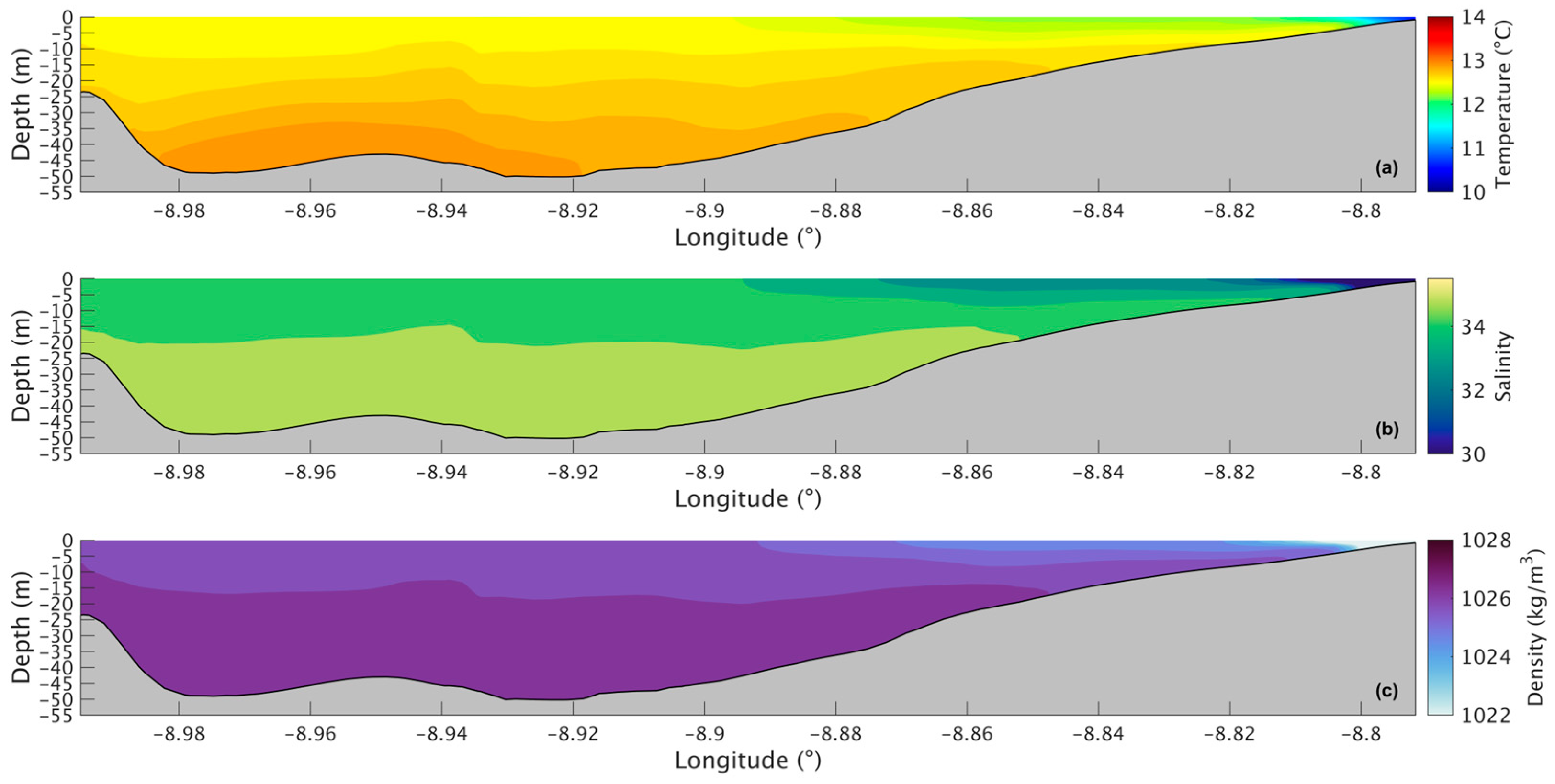
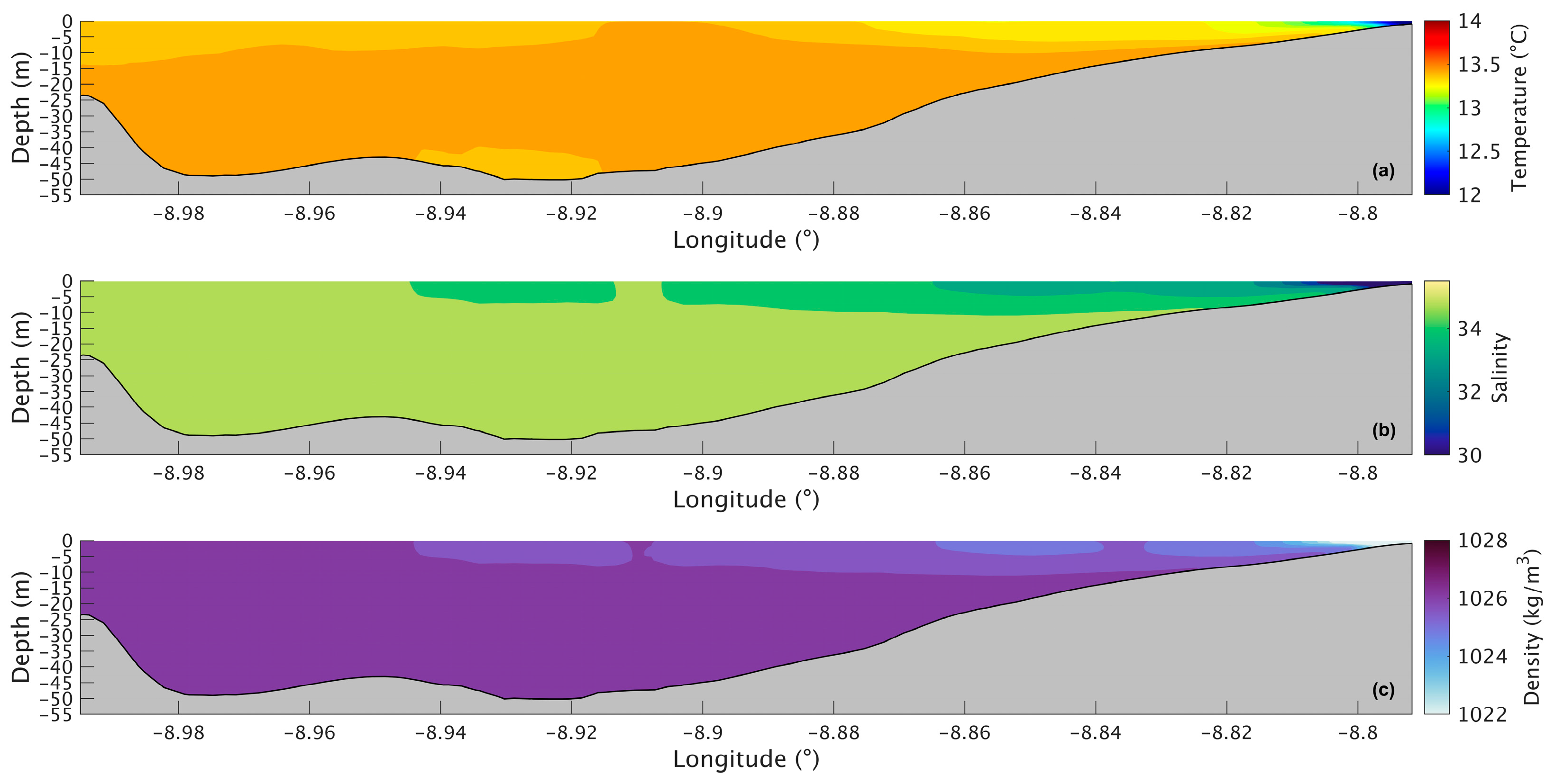
Figure 7a shows a longitudinal section of the water temperature in the present scenario. The temperature varies between 14.6 °C and 19.0 °C, with the lowest value being at the bottom in the deepest part of the Ria and the highest at the surface near the river’s mouth. The water temperature does not show much change in the upper layer, being approximately 18.5 °C. However, in the lower layers, the temperature decreases seaward, with the lowest temperature being in the deepest area of the Ria. For the future scenario (Figure 8a), similar patterns are observed, but with higher values ranging from 16.5 °C to 21 °C. The differences between the two scenarios are better illustrated in Figure 9a, where the biggest increase is 2.2 °C near the mouth of the Ria and the river’s mouth and 1.8 °C in the middle section of the Ria. The upper layer shows the smallest increase with values ranging from 1.5 °C to 1.7 °C. In the bottom layer, an increase of 1.8 °C can also be observed.

Figure 7.
Longitudinal section of water temperature (a), salinity (b), and density (c) in the present during summer’s spring tide in the Ria de Arousa.

Figure 8.
Longitudinal section of water temperature (a), salinity (b), and density (c) in the future during summer’s spring tide in the Ria de Arousa.

Figure 9.
Longitudinal section of the differences between future and present in water temperature (a), salinity (b), and density (c) during summer’s spring tide in the Ria de Arousa.
Analysing the salinity in the surface layer of the whole Ria, in the present (Figure 4b), it is verified that its value is generally 35, with a clear effect of freshwater discharge near the mouth of the River Ulla and a less notable but still observable effect of the freshwater discharge of the River Umia. In the future (Figure 5b), model results show a similar pattern compared to Figure 5b. However, Figure 6b shows the differences between the two scenarios, with an increase (around 0.5) in salinity near the river’s mouth, and as for the rest of the Ria, a decrease of approximately 0.3 was found.
The longitudinal section of the salinity (Figure 7b) shows smaller values (34.7) near the river’s mouth and an increase to 35.3 at the surface and to 35.5 in the deepest part of the Ria. Salinity values are highest in the bottom layer near the ocean and lowest in the surface layers near the river’s mouth. In the future (Figure 8b), there is a very small difference near the river’s mouth (−0.15), and the biggest decrease (0.25) is predicted by the model in the inner section and outer sections of the Ria (Figure 9b). In the middle section of the Ria, a decrease of 0.2 can be observed, and in the bottom layer the smallest decrease of 0.1 can be identified.
The map of surface density in the present scenario (Figure 4c) shows lower values near the river’s mouth (1024 kg/m3), which increase downstream due to the effect of oceanic water, which is denser than freshwater from rivers. In the future (Figure 5c), a similar pattern is foreseen but with higher density near the river’s mouth. Figure 6c shows an increase of 1.0 kg/m3 in that area and a decrease (between 0.5 and 1.0 kg/m3) in the Ria’s outer section.
The longitudinal density section (Figure 7c) shows values of 1024 kg/m3 near the river, which increases to 1025.3 kg/m3 at the surface and 1026.5 kg/m3 in the deepest area of the Ria. The stratification is also noticeable, which is to be expected under upwelling conditions. In the future (Figure 8c), a similar stratification is predicted but with lower density values. The difference between scenarios (Figure 9c) follows a similar pattern to those presented for water temperature and salinity, where the biggest decrease occurs in the inner and outer sections, with a variation of 0.75 kg/m3 and 0.65 kg/m3 in the middle section. The bottom layer shows smaller decreases, with changes between 0.65 kg/m3 in the shallow area and 0.50 kg/m3 in the deepest part. In Figure 6c, an increase near the river mouth is observed; however, this increase is not present in Figure 9c because the longitudinal section selected (as shown in Figure 1a) does not extend to the areas closest to the river mouth.
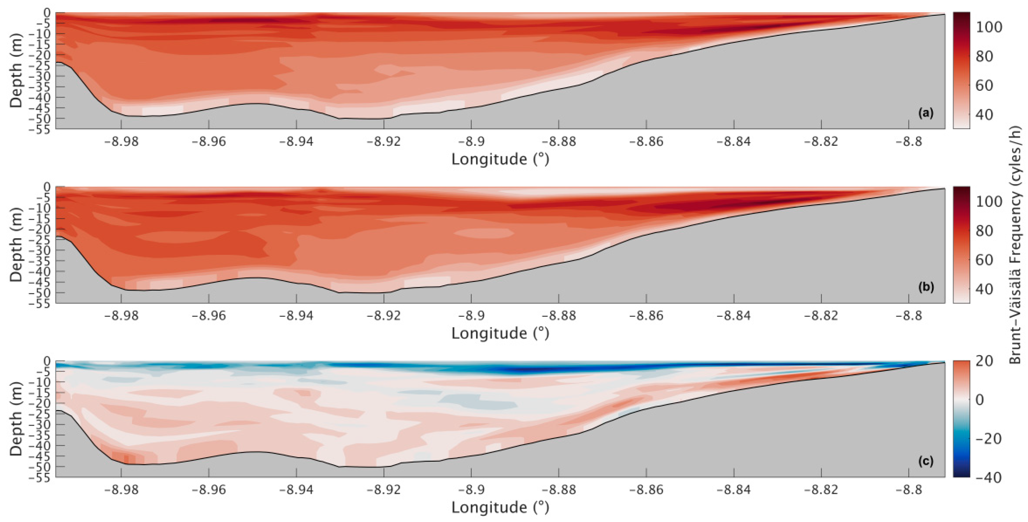
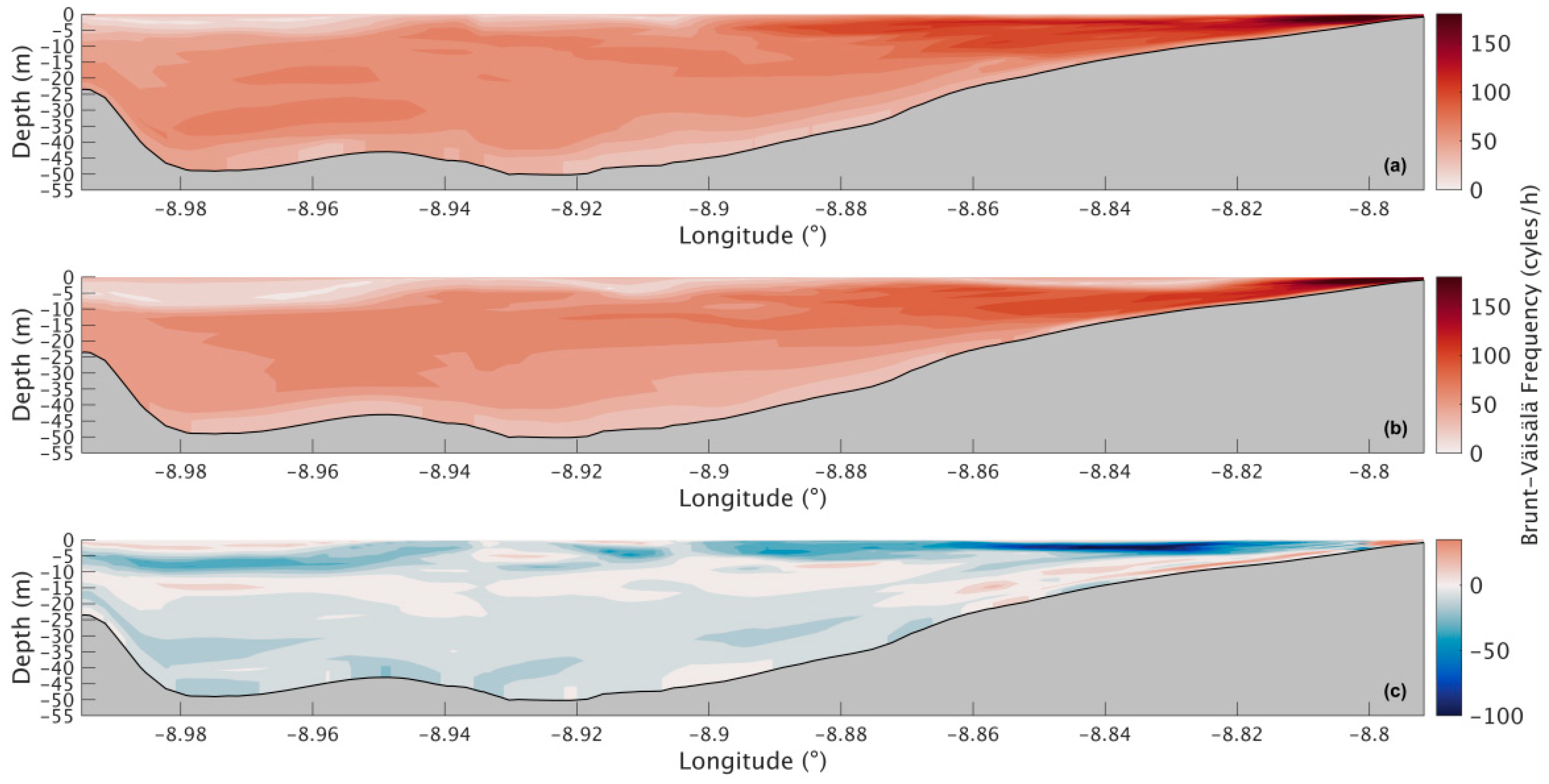
The Brunt–Väisälä frequency in the present scenario (Figure 10a) is higher at the surface, reaching 94 cycles/h, and decreases in depth, with 34 cycles/h at the bottom. For the future scenario (Figure 10b), a similar stratification pattern is predicted, where the top layers are more stratified than the lower ones, with slightly higher values in the middle and bottom layers and lower values in the surface layer near the river’s mouth (Figure 10c). The decrease in the upper layer is around 26 cycles/h, and near the bottom is where the increases will be higher, reaching 20 cycles/h.
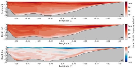
Figure 10.
Longitudinal sections of the Brunt–Väisälä frequency during summer’s spring tide for the present (a) and future (b) scenario and for the difference between the two scenarios (c) in the Ria de Arousa.
Although only one climate model and scenario were used [27], the internal variability of the system was estimated by calculating the standard deviation (or confidence intervals) of hourly values over the summer spring tide simulation period (Table 2). Table 2 shows that the temperature in the whole domain increased from a present-day mean of 18.00 ± 0.05 °C to a future mean of 19.93 ± 0.05 °C. Salinity showed a decline, from 34.97 ± 0.03 ppt to 34.69 ± 0.04 ppt. Density decreased from 1025.24 ± 0.03 kg/m3 to 1024.53 ± 0.04 kg/m3. Finally, the Brunt–Väisälä frequency (N) decreased slightly, from 75.30 ± 0.83 cycles/h to 72.02 ± 0.79 cycles/h. These results indicate a consistent trend of warming and freshening of the water column under the future scenario, leading to a reduction in water density and stratification.
Table 2.
Mean and 95% confidence interval for summer’s spring tide for the present, future, and difference between the two (Future–Present).
3.1.2. Winter’s Spring Tide
Figure 11a shows a map of the surface water temperature in the Ria de Arousa during winter spring tide for the present scenario. The lowest temperatures can be seen near the mouth of the River Ulla (8 °C), the innermost section, as well as in the area surrounding Toxa Island, showing temperature values of 11.5 °C. The rest of the Ria shows values between 12 °C and 13 °C, increasing seaward.
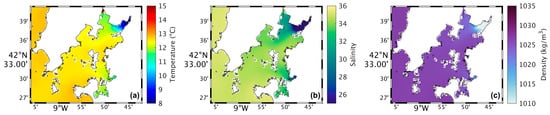
Figure 11.
Map of surface water temperature (a), salinity (b), and density (c) in the present during winter’s spring tide in the Ria de Arousa.
In the future (Figure 12a), the temperature will be higher in all of the Ria, with higher increases near the River Ulla’s mouth (Figure 13a), with an increase of 2 °C, and lower near the ocean, with an increase of only 1 °C.

Figure 12.
Map of surface water temperature (a), salinity (b), and density (c) in the future during winter’s spring tide in the Ria de Arousa.

Figure 13.
Map of the differences between future and present in surface water temperature (a), salinity (b), and density (c) during winter’s spring tide in the Ria de Arousa.
Figure 14a shows the water temperature longitudinal section for the present, and from its analysis, it is observed that the water temperature is lowest in the innermost part of the Ria with a value of 10 °C and that water gradually gets warmer moving seaward, reaching 12.5 °C at the surface and 12.9 °C at the bottom.
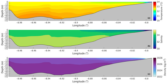
Figure 14.
Longitudinal section of water temperature (a), salinity (b), and density (c) in the present during winter’s spring tide in the Ria de Arousa.
In the future (Figure 15a), a similar pattern will be observed but with higher values at the surface (13.41 °C) and in the innermost section (12 °C) and lower values in the deepest area (13.47 °C). Therefore, the changes (Figure 16a) are higher at the surface near the river, with an increase of 1.2 °C, and lower in the deepest area of the Ria, with an increase of only 0.5 °C. The surface layer shows smaller increases moving seaward, reaching a value of 0.8 °C near the Ria’s entrance.
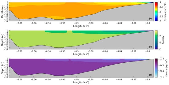
Figure 15.
Longitudinal section of water temperature (a), salinity (b), and density (c) in the future during winter’s spring tide in the Ria de Arousa.
Figure 16.
Longitudinal section of the differences between future and present in water temperature (a), salinity (b), and density (c) during winter’s spring tide in the Ria de Arousa.
Figure 11b represents the salinity in the surface layer of the whole Ria for the present, and from its analysis, it is found that the salinity is much lower compared to what was observed in the summer. Near the mouths of the rivers Umia and Ulla, the salinity is 25, increasing to approximately 30 moving away downstream, so that the inner section is less salty and the area near the ocean is saltier. In the future (Figure 12b), a similar pattern will occur but with less intensity near the river’s mouth as freshwater input is expected to decrease. Figure 13b shows the biggest increase (1) in the inner section of the Ria, while the rest of the Ria presents changes of 0.3.
During winter spring tide, in the present scenario (Figure 14b), the salinity increases longitudinally and with depth, with values of 30 near the river that increase to 34.4 in the surface layer and 35.4 in the bottom layer. The effect of the higher freshwater runoff mentioned above is also identifiable in this case as the salinity is lower overall. In the future (Figure 15b), the influence of the river discharge will be less predominant but still present, which is consistent with the expected decrease in freshwater runoff. The rest of the Ria presents values of 34.5 at the surface and 35.5 at the bottom. The salinity will increase (Figure 16b) upstream with a maximum value of 1. The smaller increase will be in the deepest area of the Ria, with a value of only 0.15, while the rest of the Ria presents values of 0.3.
The map of surface density in the present (Figure 11c) shows that the values are lower near the river’s mouth (1010 kg/m3) and then increase to 1025 kg/m3 for the rest of the Ria. In the future (Figure 12c), the same will be observed but with higher density in the inner section, as Figure 13c shows an increase of 1 kg/m3 in that area, while the rest of the Ria shows maximum changes of 0.2 kg/m3.
The density longitudinal section in the present (Figure 14c) shows that the Ria is vertically homogeneous in the middle and outer sections, with density values ranging from 1026 kg/m3 to 1026.7 kg/m3, and has some partial stratification in the inner section due to the higher discharges of freshwater from the River Ulla. The density is lower at the surface and higher in the bottom layers, and in the future (Figure 15c) a similar pattern will be identified but with slightly higher density values. As the river discharges are expected to decrease, the influence of less dense freshwater will also be less noticeable, making the overall density of the Ria higher. The increase will be higher near the river’s mouth (Figure 16c), with density values increasing up to 2 kg/m3, and a decrease moving seaward in the upper layer. The lower layers show an increase of 0.1 kg/m3 in most of the Ria.
The density during the winter season shows notable differences when compared to the summer. While in the summer it showed stratification, in the winter it is mainly homogenous. The freshwater discharges are higher in the winter; however, in the future, the freshwater discharges will decrease, and that will be reflected in an increase in salinity and density.
The Brunt–Väisälä frequency during winter’s spring tide (Figure 17) shows higher stratification than observed in the summer. In the present (Figure 17a), it is observed that the N values are higher at the surface and in the inner section of the Ria, reaching 200 cycles/h, and moving seaward, the upper layers get less stratified, showing lower N values. In the middle layers, N also decreases with latitude, reaching 60 cycles/h near the mouth of the Ria. The bottom layer also shows lower N values with approximately 30 cycles/h. Results for the future are shown in Figure 17b, and there will be an overall decrease in the Brunt–Väisälä frequency; however, patterns like those described in the present scenario are observed. Analysing the difference between the two scenarios (Figure 17c), it is observed in more detail that the N will mostly decrease, especially near the mouth of the river, where the decrease is as much as 99 cycles/h, and that decrease lessens downstream. The bottom layer shows a small increase in the shallowest area of approximately 31 cycles/h, while the rest of the Ria mainly shows decreases with higher values in the surface layers (30 cycles/h).

Figure 17.
Longitudinal sections of the Brunt–Väisälä frequency during winter’s spring tide for the present (a) and future (b) scenario and for the difference between the two scenarios (c) in the Ria de Arousa.
The means with a 95% confidence interval for winter’s spring tide (Table 3) show that the temperature in the whole domain increased from a present-day mean of 12.13 ± 0.03 °C to a future mean of 13.08 ± 0.03 °C. Salinity increased from 30.89 ± 0.25 ppt to 31.08 ± 0.27 ppt, and density decreased slightly from 1023.35 ± 0.19 kg/m3 to 1023.33 ± 0.21 kg/m3. The Brunt–Väisälä frequency shows a decrease from 78.50 ± 1.34 cycles/h to 71.86 ± 1.28 cycles/h. In the winter spring tide, the system exhibited the same general behaviour as in summer, including a trend in temperature increase, salinity decrease, and reduced stratification. However, the range of the confidence intervals between the two scenarios varied between summer and winter, with winter scenarios exhibiting larger margins of error across all variables.
Table 3.
Mean and 95% confidence interval for winter’s spring tide for the present, future, and difference between the two (future–present).
3.2. Residual Circulation
In this section, the longitudinal sections of the residual circulation in Ria de Arousa are analysed for the present and future scenarios during summer and winter.
3.2.1. Summer
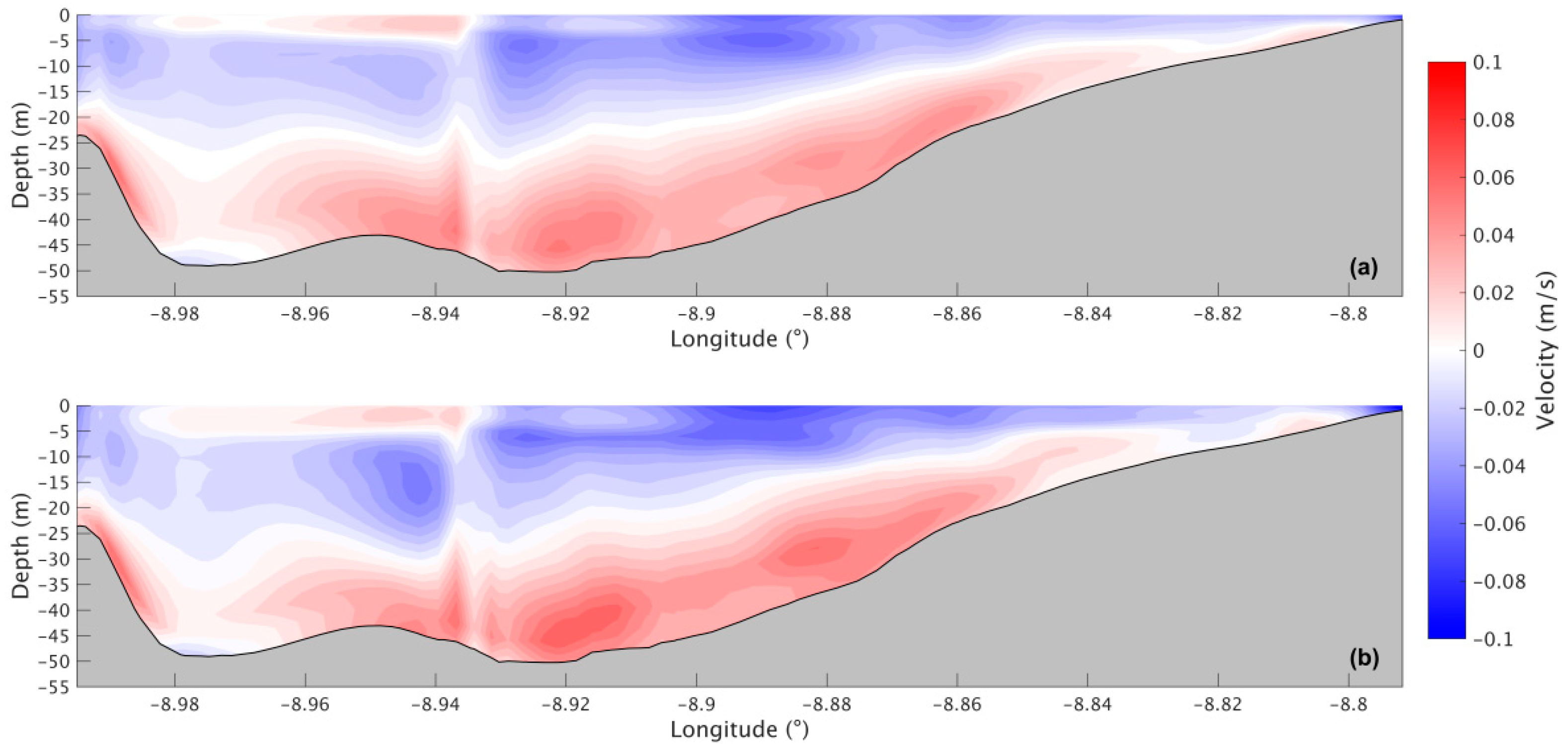
In the Ria de Arousa, during the summer for the present scenario (Figure 18a), a positive circulation can be observed, where freshwater leaves the Ria through the upper layers and saltwater enters the Ria near the bottom. Upper-layer velocities range from −0.013 m/s to −0.056 m/s, with the highest velocities found in the deepest part of the Ria. The bottom layer shows values ranging from 0.007 m/s near the centre of the Ria to 0.050 m/s near the mouth of the River Ulla and the connection with the ocean. For the future scenario (Figure 18b), model results suggest an intensification in the circulation with an increase of 0.01 m/s in both layers.

Figure 18.
Residual circulation during the summer for the present (a) and future (b) scenarios in the Ria de Arousa.
3.2.2. Winter
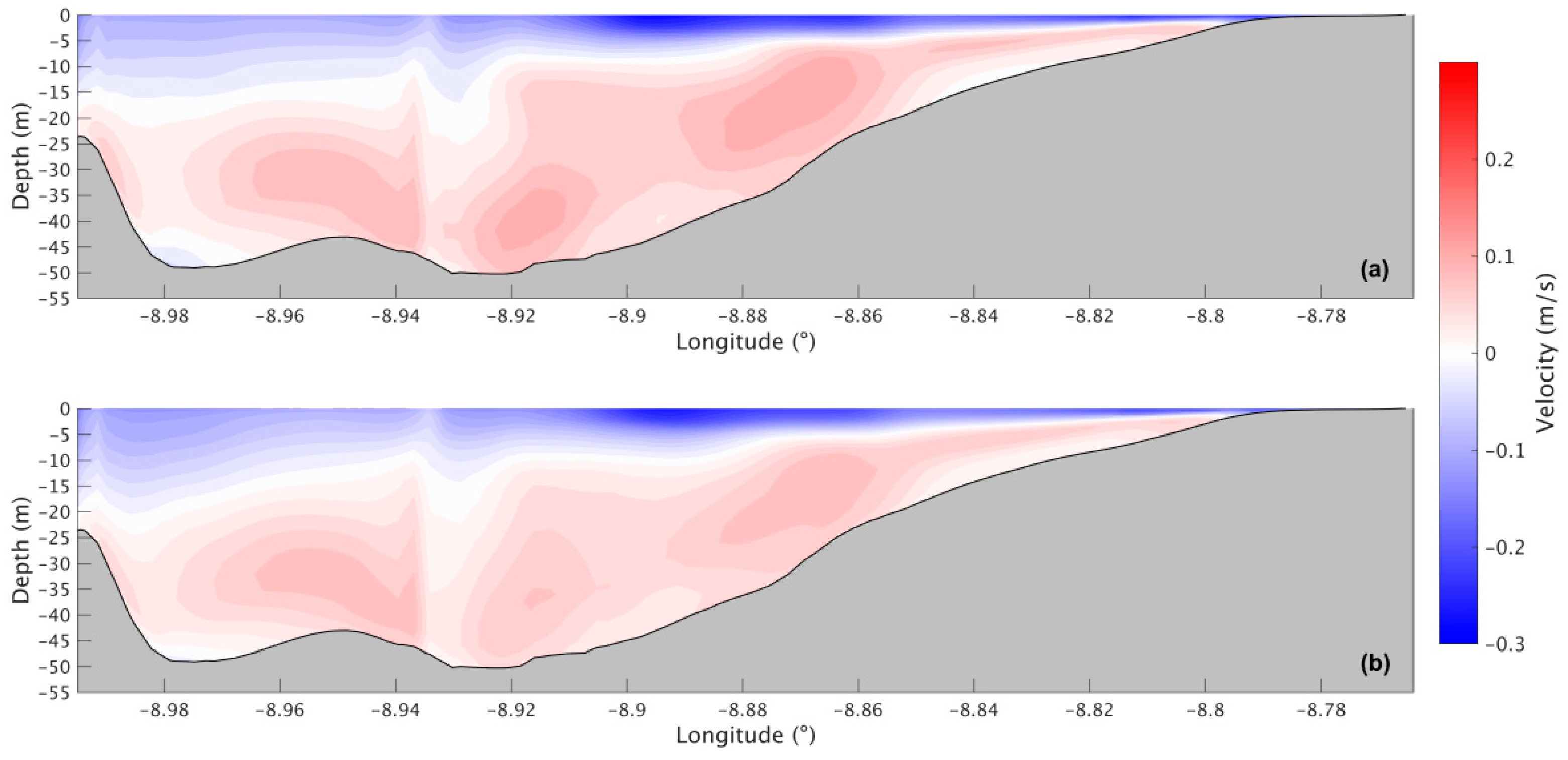
During the winter, the circulation pattern for the present scenario (Figure 19a) is also positive as in summer, with higher velocities (−0.3 m/s) in the upper layer and lower velocities (0.05 m/s) near the bottom. In the future scenario (Figure 19b), results suggest that the upper layer will show no change, and the lower layer is going to weaken in the future, with velocity values decreasing.

Figure 19.
Residual circulation during the winter for the present (a) and the future (b) scenarios in the Ria de Arousa.
In further comparing the two seasons, it is observed that the upper layer is deeper in the summer, reaching −20 m. At the same time, in the winter, the upper layer can be found at depths only ranging from −10 to −15 m, albeit with higher velocities than in the summer season.
4. Discussion
The results generally indicate a clear trend of warming in the water column under future scenarios. This change leads to a decrease in water density and stratification. Although the standard deviations are relatively small, the differences between the present and future mean values are greater than the internal variability. This suggests that the projected changes are significant and robust within the context of this model configuration.
Near the mouths of the rivers, the water temperature, salinity, and density show patterns that result from the influence of freshwater discharged, which is less saline and dense than ocean water. Near the mouth of the Ria, the influence of the more saline marine water is also clear. Similar to what was found by [7], in the summer, bottom water temperatures decrease compared with the winter, which could be a result of the intrusion of ENACW, a colder water mass. In the winter, the water temperature near the bottom tends to be warmer than at the surface, indicating a typical winter thermal inversion, which is consistent with what was observed by [40] in the Ria de Pontevedra. The evident decrease in salinity during the winter is connected to the higher freshwater discharges due to higher precipitation. The effects of higher freshwater inputs are more evident in the Ria de Arousa, as this Ria has the highest freshwater input of all the Rias Baixas [6]. In the climate change scenario considered, the results show that the water temperature will increase in both seasons, with a bigger increase in the summer when compared to the winter. In the summer, the biggest increases are found near the mouth of the Ria and the mouth of the river; this is also where the biggest decrease in density is found. In the winter, the increase is primarily near the mouth of the river, likely due to an increase in the water temperature of the freshwater runoff. Salinity will decrease in the summer, with the biggest decrease being in the deepest part of the Ria. In the winter, an increase in salinity and density can be observed in the areas closest to the river’s mouth, as freshwater discharges are expected to decrease with climate change.
Overall, in the winter, the Brunt–Väisälä frequency shows higher values in the innermost section, closer to the river’s mouth, and lower values near the ocean. In the summer the surface layers appear to have constant values, but N decreases with depth. This is consistent with previous findings [1]. That study calculated and averaged the Brunt–Väisälä frequency through the water column to determine the stratification of the Rias Baixas and found that the innermost part of the Rias is more stratified than the outermost one, as it can be observed for both the historical and future periods considered in their study. In the future, a general decrease in stratification is expected in the winter, and in the summer a big decrease in the surface layer is observed, while the rest of the layers will slightly increase or suffer no stratification changes. Ref. [1] also found an increase in the future stratification during the summer, with these changes being lower in northern shores and, especially, in the areas most influenced by river discharge.
The positive residual circulation pattern identified, where freshwater exits the Ria through the upper layer and saltier water enters through the bottom, was described in the Rias Baixas in various studies [7,41]. Although in the future there will be changes in the intensity of the bottom inflow and surface outflow currents, the positive circulation pattern will be maintained in all cases. The outflow surface velocity values are higher in the winter, indicating that the circulation is stronger because it is enhanced with increasing freshwater runoff, in agreement with the findings of [39,42] for the Ria de Vigo. In the future, there will be an overall strengthening of the circulation pattern in the summer and a weakening in the winter. The weakening in the winter can be explained by the expected decrease in freshwater runoff and therefore in the outflow surface current. These changes may lead to implications in the long-term transport of sediment, nutrients, and organic matter.
As stated previously, Ria de Arousa is the biggest production area of Mytilus spp. aquaculture rafts in the Rias Baixas. The main mussel species produced is the Mytilus galloprovincialis, better known as the Mediterranean Mussel [3]. This species shows its higher growth rates at water temperatures between 10 °C and 20 °C, with high levels of mortality at 24 °C [43,44]. In terms of salinity, it can survive from 20 to 36, although its highest growth rates are found for salinity values over 34 [43,44,45]. The model’s results show that in most of the Ria, the surface water temperature will exceed 20 °C in the future during summer, which may hinder the mussels’ optimal growth. Surface salinity does not show a significant change in the future during summer, remaining at 35 for most of the Ria. In the winter, values are generally lower but in both cases still in the acceptable range for mussel survival.
This study gave some insights about the present and future hydrodynamics of the Ria de Arousa; however, it has some limitations. One of them is the performance of the atmospheric model, namely, for the wind speed variable, whose predictions show some inaccuracies. Another limitation regards the limited exploitation of climate change scenarios, as this study only considered the SSP5-8.5 scenario. So, the simulation and analysis of more scenarios would have been beneficial to assess the impact of climate changes in the Ria de Arousa hydrodynamics, as it would consider a bigger range of possibilities and therefore allow for better preparedness and mitigation strategies. Despite the inclusion of 95% confidence intervals to represent internal variability during the simulation period, it is important to acknowledge that these estimates are based on a single climate model, scenario (SSP5-8.5), and tidal condition (spring tide). Therefore, these intervals do not account for additional sources of uncertainty, such as model structural differences, scenario selection, or boundary forcing conditions. Therefore, while the results provide a useful indication of likely trends, the precise magnitude and timing of projected changes should be interpreted with caution. Future studies incorporating multiple climate models and scenarios would allow a more robust quantification of uncertainty. The exploitation of climatologic results could also be considered a limitation of this study, as this may lead to losses in the analysis of short-term variability patterns.
5. Conclusions
The Delft3D hydrodynamic model was applied to the Ria de Arousa, with CMIP6’s MPI-ESM1-2-HR model results imposed as boundary conditions, to understand the thermohaline properties and residual circulation during two seasons (summer and winter) and to assess the changes between the present and a future climate change scenario.
The results show that water temperature in the summer is higher at the surface and lower near the bottom, which could be due to the intrusion of cold water from the ENAWC. The model results show that this pattern will be maintained in the future, although with higher values, as the water temperature is expected to increase around 2.5 °C. In the winter, the water at the bottom is warmer than at the surface, indicating a typical winter thermal inversion. The influence of freshwater runoff is also more noticeable during this season due to higher precipitation. In the future, the water temperature will also increase, although the increase will be smaller than in summer, only increasing between 0.5 and 1.0 °C.
Salinity is lower in the areas near the river’s mouth, due to freshwater discharge, and increases downstream to approximately 35 near the inlets. During the summer, it shows higher values near the bottom, which could be due to the presence of ENAWC. In the winter, the values near the river’s mouth are lower compared to the summer, and the middle and outer sections of the Ria appear to have similar salinities. In the future, salinity will decrease by approximately 0.2 during the summer. In the winter, the salinity showed an increase in the future scenario especially in the areas near the river’s mouth, as freshwater discharges are expected to decrease; results show increases of 0.3 mostly near the river’s mouth and a small decrease in the deepest area.
The water density during the summer decreases upstream due to the influence of freshwater discharges, while vertically it shows higher values at the bottom, which could be due to ENAWC intrusion. During the winter, it also decreases upstream, reaching a lower value compared to the summer, but vertically the water density is more homogeneous. In the future, the water density is vertical homogeneous during the winter (downwelling period) and stratified during the summer (upwelling period). In the winter, it will increase by 0.1 kg/m3 in the upper layers, while the bottom layers have no change. In the summer, the water density will decrease with values of around 0.7 kg/m3.
Concerning the Brunt–Väisälä frequency, in winter, stronger values are found in the innermost section closer to the river’s mouth, showing higher stratification of the water column, and lower values near the ocean, indicating less stratification. In the summer, the surface layers appear to have the same values, but N decreases with depth, indicating that the water column is less stable at depth. In the future, during the winter, there will be mainly a decrease in Brunt–Väisälä frequency, while in the summer, there will be a big decrease in the surface layer and a small increase or no change in the rest of the water column. In the winter, it will decrease by 20 cycles/h.
The residual circulation shows a positive circulation pattern. Freshwater leaves the Ria through the upper layers and saltwater enters the Ria through the bottom. In the future, the residual circulation pattern will strengthen in the summer and weaken in the winter due to a decrease in freshwater runoff. The positive circulation pattern observed in the present will be maintained in the future, showing that although climate change will impact its intensity, it will not cause an inversion of the present typical circulation pattern.
Future work could include a study on the comparative effect of variables such as wind and freshwater runoff on the patterns observed in Ria de Arousa hydrodynamics to determine the main driving factor of the local circulation. It would also be beneficial to attempt the identification of the Western Iberian Buoyant Plume impact inside the Ria. Additionally, some works have found an inversion of circulation in the Rias Baixas; therefore, further work could focus on the identification of the causes and patterns associated with that circulation inversion. Finally, as the Ria de Arousa sustains very important aquaculture activities, it would be beneficial to study the effects of these changes on all the species cultivated, as well as on the other species that inhabit the Rias Baixas.
Author Contributions
Conceptualisation, C.R., M.C.S., H.P., A.R., I.A. and J.M.D.; methodology, C.R., M.C.S., H.P., I.A. and A.R.; validation, C.R., M.C.S. and A.R.; formal analysis, C.R., M.C.S. and J.M.D.; investigation, C.R. and M.C.S.; resources, J.M.D.; writing—original draft preparation, C.R.; writing—review and editing, C.R., M.C.S., H.P., A.R., I.A. and J.M.D. All authors have read and agreed to the published version of the manuscript.
Funding
The authors acknowledge financial support to UID Centro de Estudos do Ambiente e Mar (CESAM) + LA/P/0094/2020. The Portugal Space funded this work under the project “SMART”.
Data Availability Statement
The original contributions presented in this study are included in the article. Further inquiries can be directed to the corresponding author.
Conflicts of Interest
The authors declare no conflicts of interest.
References
- Des, M.; Gómez-Gesteira, M.; deCastro, M.; Gómez-Gesteira, L.; Sousa, M.C. How can ocean warming at the NW Iberian Peninsula affect mussel aquaculture? Sci. Total Environ. 2020, 709, 136117. [Google Scholar] [CrossRef] [PubMed]
- Vaz, L.; Sousa, M.C.; Gómez-Gesteira, M.; Dias, J.M. A habitat suitability model for aquaculture site selection: Ria de Aveiro and Rias Baixas. Sci. Total Environ. 2021, 801, 149687. [Google Scholar] [CrossRef] [PubMed]
- Silva, A.F.; Sousa, M.C.; Bernardes, C.; Dias, J.M. Will Climate Change Endangers the Current Mussel Production in the Rias Baixas. J. Aquac. Fish. 2017, 1, 1. [Google Scholar] [CrossRef]
- Sousa, M. Modelling the Minho River Plume Intrusion into the Rias Baixas. Ph.D. Thesis, Universidade de Aveiro, Aveiro, Portugal, 2013. [Google Scholar]
- Rosón, G.; Pérez, F.F.; Alvarez-Salgado, X.A.; Figueiras, F.G. Variation of both thermohaline and chemical properties in an estuarine upwelling ecosystem: Ria de arousa: I. Time evolution. Estuar. Coast. Shelf Sci. 1995, 41, 195–213. [Google Scholar] [CrossRef]
- Río-Barja, F.; Rodríguez-Lestegás, F. As Augas de Galicia; Consello de Cultura: Santiago de Compostela, Spain, 1992. [Google Scholar]
- Alvarez, I.; deCastro, M.; Gomez-Gesteira, M.; Prego, R. Inter- and intra-annual analysis of the salinity and temperature evolution in the Galician Rías Baixas-ocean boundary (northwest Spain). J. Geophys. Res. Oceans 2005, 110, C04008. [Google Scholar] [CrossRef]
- Barton, E.D.; Largier, J.; Torres, R.; Sheridan, M.; Trasviña, A.; Souza, A.; Pazos, Y.; Valle-Levinson, A. Coastal upwelling and downwelling forcing of circulation in a semi-enclosed bay: Ria de Vigo. Prog. Oceanogr. 2015, 134, 173–189. [Google Scholar] [CrossRef]
- Otto, L. Oceanography of the Ria de Arosa (NW Spain); University of Leiden: Leiden, The Netherlands, 1975; 210p. [Google Scholar]
- Des, M.; Fernández-Nóvoa, D.; deCastro, M.; Gómez-Gesteira, J.L.; Sousa, M.C.; Gómez-Gesteira, M. Modeling salinity drop in estuarine areas under extreme precipitation events within a context of climate change: Effect on bivalve mortality in Galician Rías Baixas. Sci. Total Environ. 2021, 790, 148147. [Google Scholar] [CrossRef]
- Tokarska, K.B.; Stolpe, M.; Sippel, S.; Fischer, E.; Smith, C.; Lehner, F.; Knutti, R. Past warming trend constrains future warming in CMIP6 models. Sci. Adv. 2020, 6, 9549–9567. [Google Scholar] [CrossRef]
- Calvin, K.; Dasgupta, D.; Krinner, G.; Mukherji, A.; Thorne, P.W.; Trisos, C.; Romero, J.; Aldunce, P.; Barrett, K.; Blanco, G.; et al. IPCC, 2023: Climate Change 2023: Synthesis Report; IPCC: Geneva, Switzerland, 2023. [Google Scholar] [CrossRef]
- Baptistelli, S.C. Hydrodynamic Modeling: Application of Delft3D-FLOW in Santos Bay, São Paulo State, Brazil. In Recent Progress in Desalination, Environmental and Marine Outfall Systems; Springer International Publishing: Cham, Switzerland, 2015; pp. 307–332. [Google Scholar] [CrossRef]
- Dias, J.M.; Lopes, J.F.; Dekeyser, I. Lagrangian transport of particles in Ria de Aveiro lagoon, Portugal. Phys. Chem. Earth Part B Hydrol. Oceans Atmos. 2001, 26, 721–727. [Google Scholar] [CrossRef]
- Elias, E.P.L.; Walstra, D.J.R.; Roelvink, J.A.; Stive, M.J.F.; Klein, M.D. Hydrodynamic Validation of Delft3D with Field Measurements at Egmond. In Coastal Engineering 2000; American Society of Civil Engineers: Reston, VA, USA, 2001; pp. 2714–2727. [Google Scholar] [CrossRef]
- Mendes, J.; Ruela, R.; Picado, A.; Pinheiro, J.P.; Ribeiro, A.S.; Pereira, H.; Dias, J.M. Modeling Dynamic Processes of Mondego Estuary and Óbidos Lagoon Using Delft3D. J. Mar. Sci. Eng. 2021, 9, 91. [Google Scholar] [CrossRef]
- Tu, L.X.; Thanh, V.Q.; Reyns, J.; Van, S.P.; Anh, D.T.; Dang, T.D.; Roelvink, D. Sediment transport and morphodynamical modeling on the estuaries and coastal zone of the Vietnamese Mekong Delta. Cont. Shelf Res. 2019, 186, 64–76. [Google Scholar] [CrossRef]
- Des, M.; deCastro, M.; Sousa, M.C.; Dias, J.M.; Gómez-Gesteira, M. Hydrodynamics of river plume intrusion into an adjacent estuary: The Minho River and Ria de Vigo. J. Mar. Syst. 2019, 189, 87–97. [Google Scholar] [CrossRef]
- Iglesias, G.; Carballo, R. Seasonality of the circulation in the Ría de Muros (NW Spain). J. Mar. Syst. 2009, 78, 94–108. [Google Scholar] [CrossRef]
- Carballo, R.; Iglesias, G.; Castro, A. Numerical model evaluation of tidal stream energy resources in the Ría de Muros (NW Spain). Renew. Energy 2009, 34, 1517–1524. [Google Scholar] [CrossRef]
- Iglesias, G.; Carballo, R.; Castro, A. Baroclinic modelling and analysis of tide- and wind-induced circulation in the Ría de Muros (NW Spain). J. Mar. Syst. 2008, 74, 475–484. [Google Scholar] [CrossRef]
- Carballo, R.; Iglesias, G.; Castro, A. Residual circulation in the Ría de Muros (NW Spain): A 3D numerical model study. J. Mar. Syst. 2009, 75, 116–130. [Google Scholar] [CrossRef]
- Sousa, M.C.; Vaz, N.; Alvarez, I.; Gomez-Gesteira, M.; Dias, J.M. Modeling the Minho River plume intrusion into the Rias Baixas (NW Iberian Peninsula). Cont. Shelf Res. 2014, 85, 30–41. [Google Scholar] [CrossRef]
- Alvarez, I.; deCastro, M.; Gomez-Gesteira, M.; Prego, R. Hydrographic behavior of the Galician Rias Baixas (NW Spain) under the spring intrusion of the Miño River. J. Mar. Syst. 2006, 60, 144–152. [Google Scholar] [CrossRef]
- Liu, H.; Song, Z.; Wang, X.; Misra, V. An ocean perspective on CMIP6 climate model evaluations. Deep. Sea Res. Part II Top. Stud. Oceanogr. 2022, 201, 105120. [Google Scholar] [CrossRef]
- Liu, Y.; Cheng, L.; Pan, Y.; Tan, Z.; Abraham, J.; Zhang, B.; Zhu, J.; Song, J. How Well Do CMIP6 and CMIP5 Models Simulate the Climatological Seasonal Variations in Ocean Salinity? Adv. Atmos. Sci. 2022, 39, 1650–1672. [Google Scholar] [CrossRef]
- Pereira, H.; Picado, A.; Sousa, M.C.; Alvarez, I.; Dias, J.M. Evaluation of Earth System Models outputs over the continental Portuguese coast: A historical comparison between CMIP5 and CMIP6. Ocean Model. 2023, 184, 102207. [Google Scholar] [CrossRef]
- Laurent, A.; Fennel, K.; Kuhn, A. An observation-based evaluation and ranking of historical Earth system model simulations in the northwest North Atlantic Ocean. Biogeosciences 2021, 18, 1803–1822. [Google Scholar] [CrossRef]
- Andres-Martin, M.; Azorin-Molina, C.; Shen, C.; Fernández-Alvarez, J.C.; Gimeno, L.; Vicente-Serrano, S.M.; Zha, J. Uncertainty in surface wind speed projections over the Iberian Peninsula: CMIP6 GCMs versus a WRF-RCM. Ann. N. Y. Acad. Sci. 2023. [Google Scholar] [CrossRef] [PubMed]
- Shen, C.; Zha, J.; Li, Z.; Azorin-Molina, C.; Deng, K.; Minola, L.; Chen, D. Evaluation of global terrestrial near-surface wind speed simulated by CMIP6 models and their future projections. Ann. N. Y. Acad. Sci. 2022, 1518, 249–263. [Google Scholar] [CrossRef]
- Müller, W.A.; Jungclaus, J.H.; Mauritsen, T.; Baehr, J.; Bittner, M.; Budich, R.; Bunzel, F.; Esch, M.; Ghosh, R.; Haak, H.; et al. A Higher-resolution Version of the Max Planck Institute Earth System Model (MPI-ESM1.2-HR). J. Adv. Model. Earth Syst. 2018, 10, 1383–1413. [Google Scholar] [CrossRef]
- Hundecha, Y.; Arheimer, B.; Donnelly, C.; Pechlivanidis, I. A regional parameter estimation scheme for a pan-European multi-basin model. J. Hydrol. Reg. Stud. 2016, 6, 90–111. [Google Scholar] [CrossRef]
- “Europe Climate Change—HypeWeb”. [Online]. Available online: https://hypeweb.smhi.se/explore-water/climate-change-data/europe-climate-change/ (accessed on 10 September 2023).
- Sousa, M.C.; Ribeiro, A.; Des, M.; Gomez-Gesteira, M.; deCastro, M.; Dias, J.M. NW Iberian Peninsula coastal upwelling future weakening: Competition between wind intensification and surface heating. Sci. Total Environ. 2020, 703, 134808. [Google Scholar] [CrossRef]
- Talley, L.D.; Pickard, G.L.; Emery, W.J.; Swift, J.H. Chapter 3—Physical Properties of Seawater. In Descriptive Physical Oceanography, 6th ed.; Talley, L.D., Pickard, G.L., Emery, W.J., Swift, J.H., Eds.; Academic Press: Boston, MA, USA, 2011; pp. 29–65. [Google Scholar] [CrossRef]
- Pond, S.; Pickard, G. Introductory Dynamical Oceanography; Elsevier: Amsterdam, The Netherlands, 1983. [Google Scholar] [CrossRef]
- Burchard, H.; Hetland, R.D. Quantifying the Contributions of Tidal Straining and Gravitational Circulation to Residual Circulation in Periodically Stratified Tidal Estuaries. J. Phys. Oceanogr. 2010, 40, 1243–1262. [Google Scholar] [CrossRef]
- Piedracoba, S.; Álvarez-Salgado, X.A.; Rosón, G.; Herrera, J.L. Short-timescale thermohaline variability and residual circulation in the central segment of the coastal upwelling system of the Ría de Vigo (northwest Spain) during four contrasting periods. J. Geophys. Res. Oceans 2005, 110. [Google Scholar] [CrossRef]
- Taboada, J.J.; Prego, R.; Ruiz-Villarreal, M.; Gómez-Gesteira, M.; Montero, P.; Santos, A.; Pérez-Villar, V. Evaluation of the Seasonal Variations in the Residual Circulation in the Ría of Vigo (NW Spain) by Means of a 3D Baroclinic Model. Estuar. Coast. Shelf Sci. 1998, 47, 661–670. [Google Scholar] [CrossRef]
- Álvarez, I.; deCastro, M.; Prego, R.; Gómez-Gesteira, M. Hydrographic characterization of a winter-upwelling event in the Ria of Pontevedra (NW Spain). Estuar. Coast. Shelf Sci. 2003, 56, 869–876. [Google Scholar] [CrossRef]
- Gómez-Gesteira, M.; deCastro, M.; Prego, R.; Pérez-Villar, V. An Unusual Two Layered Tidal Circulation Induced by Stratification and Wind in the Ría of Pontevedra (NW Spain). Estuar. Coast. Shelf Sci. 2001, 52, 555–563. [Google Scholar] [CrossRef]
- Prego, R.; Fraga, F. A Simple Model to Calculate the Residual Flows in a Spanish Ria. Hydrographic Consequences in the ria of Vigo. Estuar. Coast. Shelf Sci. 1992, 34, 603–615. [Google Scholar] [CrossRef]
- Anestis, A.; Lazou, A.; Pörtner, H.O.; Michaelidis, B. Behavioral, metabolic, and molecular stress responses of marine bivalve Mytilus galloprovincialis during long-term acclimation at increasing ambient temperature. Am. J. Physiol.-Regul. Integr. Comp. Physiol. 2007, 293, R911–R921. [Google Scholar] [CrossRef]
- Van Erkom Schurink, C.; Griffiths, C.L. Physiological energetics of four South African mussel species in relation to body size, ration and temperature. Comp. Biochem. Physiol. A Physiol. 1992, 101, 779–789. [Google Scholar] [CrossRef]
- Ferreira, J.; Magalhães, A. Cultivo de mexilhoes. In Aquicultura: Experiencias Brasileiras; Poli, C.R.P., Poli, A.T.B., Andreatta, E.R., Beltrame, E., Eds.; Universidade Federal de Santa Catarina: Florianopolis, Brazil, 2004. [Google Scholar]


Disclaimer/Publisher’s Note: The statements, opinions and data contained in all publications are solely those of the individual author(s) and contributor(s) and not of MDPI and/or the editor(s). MDPI and/or the editor(s) disclaim responsibility for any injury to people or property resulting from any ideas, methods, instructions or products referred to in the content. |
© 2025 by the authors. Licensee MDPI, Basel, Switzerland. This article is an open access article distributed under the terms and conditions of the Creative Commons Attribution (CC BY) license (https://creativecommons.org/licenses/by/4.0/).