Improved Online Kalman Smoothing Method for Ship Maneuvering Motion Data Using Expectation-Maximization Algorithm

Abstract

Despite the pivotal role of filtering and smoothing techniques in the preprocessing of ship maneuvering data for robust identification, persistent challenges in reconciling noise suppression with dynamic fidelity preservation have limited algorithmic advancements in recent decades. We propose an online smoothing method enhanced by the Expectation-Maximization (EM) algorithm framework that effectively extracts high-fidelity dynamic features from raw maneuvering data, thereby enhancing the fidelity of subsequent ship identification systems. Our method effectively addresses the challenges posed by heavy-tailed Student-t distributed noise and parameter uncertainty inherent in ship motion data, demonstrating robust parameter learning capabilities, even when initial ship motion system parameters deviate from real conditions. Through iterative data assimilation, the algorithm adaptively calibrates noise distribution parameters while preserving motion smoothness, achieving superior accuracy in velocity and heading estimation compared to conventional Rauch–Tung–Striebel (RTS) smoothers. By integrating parameter adaptation within the smoothing framework, the proposed method reduces motion prediction errors by 23.6% in irregular sea states, as validated using real ship motion data from autonomous navigation tests.

1. Introduction

Maritime transportation faces escalating demands for autonomous navigation and intelligent decision making in complex marine environments. Ship maneuvering systems, which are critical for collision avoidance, route optimization, and energy efficiency, heavily rely on precise state estimation amidst severe nonlinearity (e.g., hydrodynamic forces), environmental disturbances (e.g., wind/wave-induced motion), and sensor noise [1]. Traditional filtering approaches, such as the RTS smoother [2], often fail under heavy-tailed noise conditions prevalent in marine sensing (e.g., GPS jamming or sensor saturation), leading to biased trajectory reconstructions and compromised control performance [3]. For instance, inaccurate state estimation in dynamic positioning systems (DPSs) can increase fuel consumption by up to 15% and elevate accident risks in confined waterways [4]. Recent studies highlight that Student-t noise models outperform Gaussian frameworks in handling such outliers, yet real-time adaptive calibration of noise parameters remains challenging due to computational burdens and sensitivity to initialization.

To address these gaps, this work introduces an online smoothing algorithm integrating expectation maximization (EM) for adaptive noise learning. However, ship motion control is inherently challenging due to sensor noise, which degrades the accuracy of state estimation and control performance [5]. This study focuses on the critical role of smooth data processing in ship motion identification and control, where “smooth” refers to a noise-filtered dataset derived from high-frequency measurements. By applying advanced filtering techniques (e.g., extended Kalman filter [6], sliding-window least squares [7], or deep learning-based denoising [8]), we obtain a temporally consistent and physically meaningful dataset that mitigates the effects of measurement noise and transient errors. Reducing errors from measurement noise allows for more accurate vessel control and helps prevent accidents by enabling prompt responses to sudden situations [9]. Additionally, smoothed data processing optimizes navigational efficiency, minimizing unnecessary acceleration and deceleration, which leads to fuel savings and shorter travel times.

Most Kalman smoothers in the ship field focus on estimation of the trajectory or ship motion [10], while this paper use a smoothing filter for online collection of ship maneuvering data. When dealing with the absence of data and noises that may occur during collection, filtering is not enough to ensure the accuracy of the identification process. The variational Bayesian method proposed in [11] addresses real-time, low-frequency motion-state estimation for DP ships under time-varying environmental disturbances by integrating variational Bayesian inference with multiple fading factors. While it overcomes the limitations of conventional smoothing algorithms in online noise adaptation and historical data re-optimization, its computational efficiency remains inferior to that of our RTS-based post-processing approach. Ma et al. [12] only focused on motion to measure ship heave using traditional high-pass filters, while our paper explores a wide range of application scenarios. Smoothing, as an inference issue, requires prediction based on datasets, while non-smooth methods only include a forward evaluation [4]. To address the issue of identifying ship motion parameters and wave peak frequency, Liu et al. [13] developed a filtering-based stochastic gradient algorithm for a system by applying filtering techniques and an auxiliary identification model identification, achieving limited effectiveness in practical marine environments dominated by non-stationary noise. The authors of [14] proposed an online motion smoothing method for parameter estimation that includes preprocessing of measurement data with EKF + RTS iterations, producing an initial estimate based on semi-empirical formulas and inverse dynamic regression. Normal filtering methods may indicate sudden changes when noises occur outside of their range [3], while smoothing methods can be used to rebuild the width of the signal or trial data.

From an inferential perspective, data smoothing inherently represents a probabilistic inference problem requiring predictive modeling of latent state sequences [15]. This contrasts with non-smooth methods, which perform forward evaluation without uncertainty quantification [16]. Notably, smoothed estimates obtained via the Extended Kalman Filter (EKF) exhibit statistically significant accuracy improvements over conventionally filtered outputs (p < 0.05). This superiority arises from the optimal integration of a posteriori observational data through recursive Bayesian inference [17]. Online maneuvering data additionally require predictions across all time regions [18]. The extended Kalman filter (EKF) is inherently recursive and operates online, dynamically updating state estimates as new measurements arrive. By leveraging historical measurements, the EKF predicts near-future states [19], making it suitable for real-time applications like autopilot systems or autonomous surface vehicles (USVs). This limitation is resolved when conducting parameter estimation on complete time-series data, where both historical and future measurements are available. Bidirectional temporal information enhances filtering performance by enabling backward smoothing integration. Specifically, an EKF framework can be augmented with an RTS smoother to incorporate future time steps during state estimation [20]. This hybrid framework synergizes the EKF’s forward propagation with RTS’s backward recursion, achieving optimal smoothing [21]. Experiments on synthetic datasets with Student-t distributed noise confirm that the method significantly enhances state identifiability, particularly for marine vessel motion parameters, where traditional filters underperform.

In response to the degradation of state estimation accuracy in marine vessel motion control caused by non-Gaussian sensor noise, environmental disturbances, and hydrodynamic uncertainties, our paper introduces a robust Bayesian smoothing framework integrating the expectation-maximization algorithm for adaptive parameter learning and multi-source sensor data fusion, achieving enhanced motion reconstruction fidelity through iterative temporal–spatial noise suppression and dynamic model calibration. The contributions of this paper are outlined as follows:

• We propose an online data smoothing algorithm tailored for ship maneuvering test data, overcoming the limitations of traditional offline batch processing methods.
• We pioneer an adaptive noise-statistic inference framework through an alternating optimization of distribution hyperparameters Q and R, enabling dynamic Bayesian updating of noise characteristics while preserving the fidelity of system dynamics in modeling maneuvering data.
• We propose a novel framework integrating ship maneuvering system priors with adaptive noise modeling, effectively addressing Student-t noise challenges while outperforming traditional Gaussian smoothing methods in terms of dynamic fidelity.

2. Problem Formulation

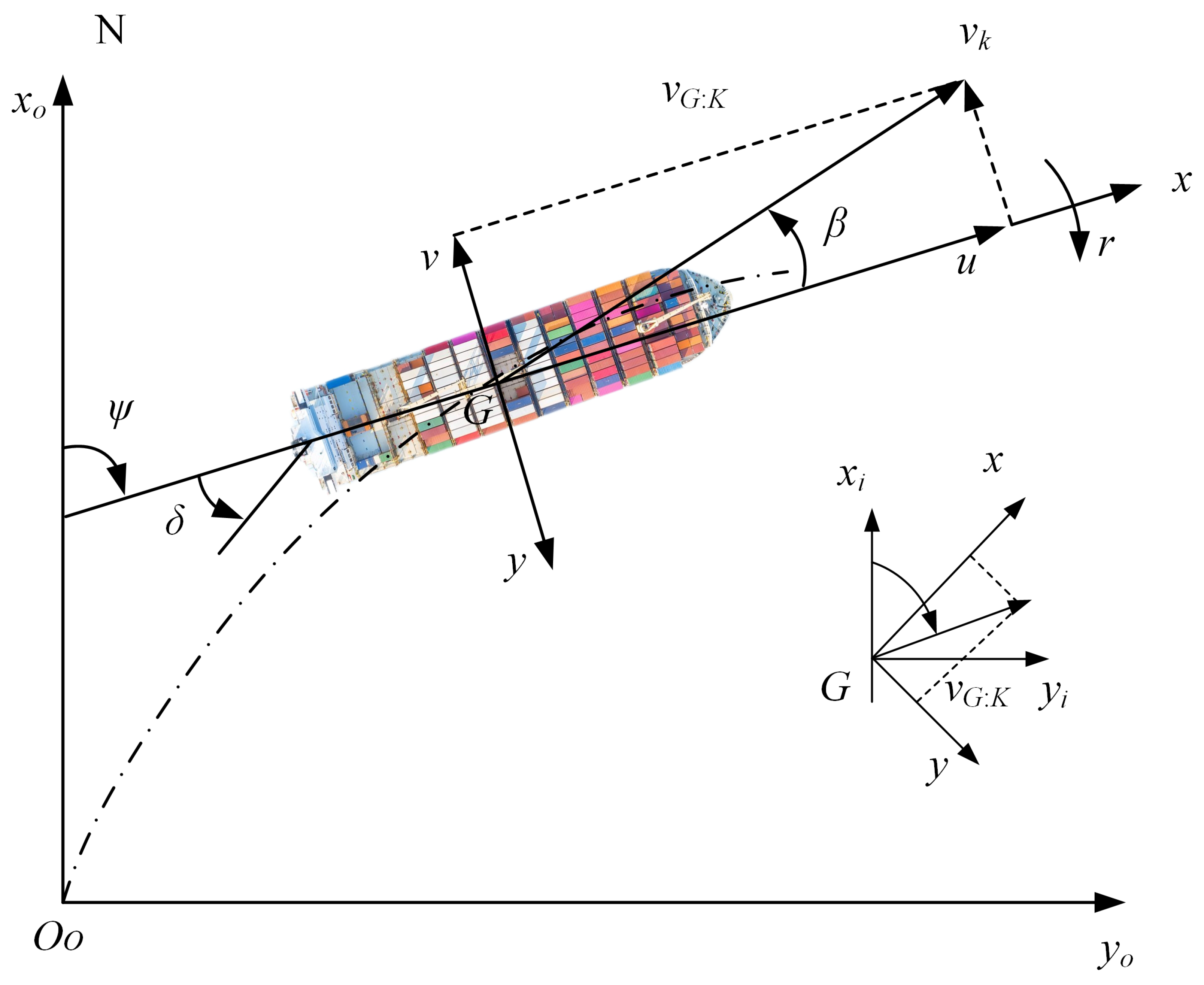
In general, a linear motion equation may be constructed to describe the motion of a ship. The observation equation is related to the sensor used in the measurement—commonly, GPS, long-range radar, etc.

The transformation relationship between the velocity vectors in the space-fixed $O_0-xy$ coordinate system and the body-fixed coordinate system ($G-x_i{y}_i$) is presented in Figure 1. To facilitate the transition between these two coordinate systems, we established a standardized transformation protocol. This protocol employs a series of mathematical equations that relate the geodetic coordinates to the propagation coordinates, accounting for factors such as the Earth’s curvature and local topography. The transformation is illustrated in Figure 1, where the axes represent the respective coordinate systems. The dashed line in the figure indicates the directional trajectory of the vessel along the specified orientation.

The ship’s kinematics are typically represented by a discrete-time, nonlinear state–space model to enable real-time processing:

$${\mathit{x}}_k=\mathbf{f}({\mathit{x}}_{k-1})+{\mathbf{s}}_k=\left[\begin{array}{c}{u}_{k-1}cos{\psi }_{k-1}-v_{k-1}sin{\psi }_{k-1}\\ u_{k-1}sin{\psi }_{k-1}+v_{k-1}cos{\psi }_{k-1}\\ {\psi }_{k-1}+r_{k-1}\Delta t\\ u_{k-1}\\ v_{k-1}\\ r_{k-1}\end{array}\right]+{\mathit{s}}_k$$

(1)

$$\begin{array}{cc}\hfill & {\mathit{z}}_k=\mathbf{h}({\mathit{x}}_k)+{\mathit{o}}_k\hfill \\ \hfill & =\left[\begin{array}{c}\Delta t\sqrt{{\left({\sum }_{i=1}^k{\dot{x}}_i\right)}^2+{\left({\sum }_{i=1}^k{\dot{y}}_i\right)}^2}\\ {\displaystyle \frac{(u_{k}sin{\psi }_k+v_{k}cos{\psi }_k){\sum }_{i=1}^k{\dot{x}}_i+(u_{k}cos{\psi }_k-v_{k}sin{\psi }_k){\sum }_{i=1}^k{\dot{y}}_i}{{\sum }_{i=1}^k{\dot{y}}_i}}\\ \sqrt{{\left({\sum }_{i=1}^k{\dot{x}}_i\right)}^2+{\left({\sum }_{i=1}^k{\dot{y}}_i\right)}^2}\\ u_k\\ v_k\\ r_k\end{array}\right]+{\mathit{o}}_k\hfill \\ \hfill \end{array}$$

(2)

where, vector ${{\mathit{x}}_k=[{\dot{x}}_{G,k},{\dot{y}}_{G,k},{\psi }_k,u_k,v_k,r_k]}^{\top }$ can be used to indicate the real-time status of the ship at moment k. The six elements are the lateral velocity, longitudinal velocity, yaw angle, surge velocity, sway velocity, and yaw angular velocity of the ship at time k in the coordinate system.

Sensor noise is often influenced by various factors, including environmental interference, equipment aging, and physical vibrations. These factors can lead to noise distributions exhibiting heavy-tailed characteristics, resulting in a higher probability of extreme values (anomalous noise). The changes in the state of the ship caused by the acceleration of the ship and the effects of the ocean current can be represented by noise ($s_k$). In order to solve the model, ${\mathit{s}}_k$ is assumed to conform to the Gaussian distribution. ${\mathit{s}}_k$ is Gaussian process noise with a zero mean value. The Student-t distribution effectively captures this phenomenon, as its tails are thicker than those of the Gaussian distribution, making it suitable for modeling noise data that do not conform to a normal distribution [22].

Here, ${\mathit{z}}_k$ is the amount observed by sensors (DGPS) at moment k, including coordinates and velocities, all of which are expressed in terms of the international system of units. Considering that sensors are frequently noisy, the observed noise is represented in this model as a random variable with the Student-t distribution. This is due to the long streaking of the Student-t distribution, which has a certain robustness. $O_k={[o_{k,1},o_{k,2},o_{k,3}]}^T\in R^3$ is the observed noise that is distributed independently from the Student-t distribution for each element, which can be expressed as $o_{k,m}\sim St(0,r_m^{-1},{\alpha }_m),m=1,2,3$. Here, $r_m^{-1}$ is the accuracy of the distribution, while ${\alpha }_m$ is the degree of freedom.

$$\{\begin{array}{c}{\dot{x}}_{G,k}=u_{k}cos{\psi }_k-v_{k}sin{\psi }_k\\ {\dot{y}}_{G,k}=u_{k}sin{\psi }_k+v_{k}cos{\psi }_k\\ \dot{{\psi }_k}=r_k\end{array}$$

(3)

where $x_k\in {\mathbb{R}}^6$ and $z_k\in {\mathbb{R}}^3$ denote the state and observation vector of $k(k=1,2,\dots ,T)$, respectively, and $f(·)$ and $h(·)$ are nonlinear and observation functions, respectively. $s_k\in {\mathbb{R}}^6$ is the Gaussian process noise with zero means, which satisfies the condition of $s_k\sim N(0,Q)$. $o_k={[o_{k,1},o_{k,2},\dots ,o_{k,m}]}^T\in {\mathbb{R}}^3$ is the observation noise of the Student-t distribution, in which each element is independently and identically distributed, that is, $o_{k,m}\sim St(0,r_m^{-1},{\alpha }_m),m=1,2,\dots ,6$. Here, $r_m^{-1}$ is the distribution accuracy, and ${\alpha }_m$ is the degree of freedom (DOF). For the sake of brevity, the declaration is expressed as follows: ${\mu }_k=x_{k-1}$; $h(x_k)={[{\mu }_{k,1},{\mu }_{k,2},\dots ,{\mu }_{k,6}]}^T$. The state matrix is $x_k={[x_{k,1},x_{k,2},\dots ,x_{k,6}]}^T$, and the observation matrix is $z_k={[z_{k,1},z_{k,2},\dots ,z_{k,6}]}^T$. The observation distribution of a given state should be taken into consideration:

$$\begin{array}{c}p({\mathit{z}}_k\mid {\mathit{x}}_k)=\prod _{m=1}^{M}St(z_{k,m}\mid {\mu }_{k,m},r_m^{-1},{\alpha }_m)\hfill \\ =\prod _{m=1}^M\int \mathcal{N}(z_{k,m}\mid {\mu }_{k,m},r_m/w_{k,m})\ast \hfill \\ Gam(w_{k,m}\mid {\alpha }_m/2,{\alpha }_m/2)d{w}_{k,m}\hfill \end{array}$$

(4)

The elements of ${\mathit{F}}_k$ are functions of the system’s dynamic parameters, not instantaneous measurements:

$${\mathit{F}}_k=\left[\begin{array}{cccccc}0& 0& -u_{k}sin{\psi }_k-v_{k}cos{\psi }_k& cos{\psi }_k& -sin{\psi }_k& 0\\ 0& 0& u_{k}cos{\psi }_k-v_{k}sin{\psi }_k& sin{\psi }_k& cos{\psi }_k& 0\\ 0& 0& 1& 0& 0& \Delta t\\ 0& 0& 0& 1& 0& 0\\ 0& 0& 0& 0& 1& 0\\ 0& 0& 0& 0& 0& 1\end{array}\right]$$

(5)

Based on the kinematic relationships in the above formula, its Jacobian matrix (${\mathit{H}}_k$) can be derived as follows:

$${\mathit{H}}_k=\left[\begin{array}{cccccc}\hfill H_{11}& \hfill H_{12}& \hfill 0& \hfill 0& \hfill 0& \hfill 0\\ \hfill H_{21}& \hfill H_{22}& \hfill 0& \hfill 0& \hfill 0& \hfill 0\\ \hfill H_{31}& \hfill H_{32}& \hfill H_{33}& \hfill H_{34}& \hfill H_{35}& \hfill 0\end{array}\right]$$

(6)

The items are expressed as follows:

$$\begin{array}{c}{H}_{11}={\displaystyle \frac{\Delta t(E(x_{G,k-1})+{\dot{x}}_k\Delta t)}{\sqrt{{(E(x_{G,k-1})+{\dot{x}}_k\Delta t)}^2+{(E(y_{G,k-1})+{\dot{y}}_k\Delta t)}^2}}}\\ H_{12}={\displaystyle \frac{\Delta t(E(y_{G,k-1})+{\dot{y}}_k\Delta t)}{\sqrt{{(E(x_{G,k-1})+{\dot{x}}_k\Delta t)}^2+{(E(y_{G,k-1})+{\dot{y}}_k\Delta t)}^2}}}\\ H_{21}={\displaystyle \frac{\Delta t(E(y_{G,k-1})+{\dot{y}}_k\Delta t)}{{(E(x_{G,k-1})+{\dot{x}}_k\Delta t)}^2+{(E(y_{G,k-1})+{\dot{y}}_k\Delta t)}^2}}\\ H_{22}=-{\displaystyle \frac{\Delta t(E(x_{G,k-1})+{\dot{x}}_k\Delta t)}{{(E(x_{G,k-1})+{\dot{x}}_k\Delta t)}^2+{(E(y_{G,k-1})+{\dot{y}}_k\Delta t)}^2}}\\ H_{31}=-{\displaystyle \frac{{(E(x_{G,k-1})+{\dot{x}}_k\Delta t)}^3+(E(y_{G,k-1})+{\dot{y}}_k\Delta t)[(E(x_{G,k-1})+{\dot{x}}_k\Delta t)E(y_{G,k-1})+(E(y_{G,k-1})+{\dot{y}}_k\Delta t){\dot{x}}_k\Delta t]}{{(E(x_{G,k-1})+{\dot{x}}_k\Delta t)}^2+{(E(y_{G,k-1})+{\dot{y}}_k\Delta t)}^2}}\\ H_{32}=-{\displaystyle \frac{{(E(y_{G,k-1})+{\dot{y}}_k\Delta t)}^3+(E(x_{G,k-1})+{\dot{x}}_k\Delta t)[(E(y_{G,k-1})+{\dot{y}}_k\Delta t)E(x_{G,k-1})+(E(x_{G,k-1})+{\dot{x}}_k\Delta t){\dot{y}}_k\Delta t]}{{(E(x_{G,k-1})+{\dot{x}}_k\Delta t)}^2+{(E(y_{G,k-1})+{\dot{y}}_k\Delta t)}^2}}\\ H_{33}=-{\displaystyle \frac{-(E(x_{G,k-1})+{\dot{x}}_k\Delta t){(u_{k}sin{\psi }_k+v_{k}cos\psi )}_k)+(E(y_{G,k-1})+{\dot{y}}_k\Delta t)(u_{k}cos\psi {\psi }_k-v_{k}sin\psi )}{{(E(x_{G,k-1})+{\dot{x}}_k\Delta t)}^2+{(E(y_{G,k-1})+{\dot{y}}_k\Delta t)}^2}}\\ H_{34}={\displaystyle \frac{(E(x_{G,k-1})+{\dot{x}}_k\Delta t)cos{\psi }_k+(E(y_{G,k-1})+{\dot{y}}_k\Delta t)sin{\psi }_k}{{(E(x_{G,k-1})+{\dot{x}}_k\Delta t)}^2+{(E(y_{G,k-1})+{\dot{y}}_k\Delta t)}^2}}\\ H_{35}={\displaystyle \frac{-(E(x_{G,k-1})+{\dot{x}}_k\Delta t)sin{\psi }_k+(E(y_{G,k-1})+{\dot{y}}_k\Delta t)cos{\psi }_k}{{(E(x_{G,k-1})+{\dot{x}}_k\Delta t)}^2+{(E(y_{G,k-1})+{\dot{y}}_k\Delta t)}^2}}\end{array}$$

(7)

By establishing and introducing a weight vector ($w_k={[w_{k,1},w_{k,2},\dots ,w_{k,M}]}^T$) that is independent of the state ($x_k$) into the model, the prior distribution can be expressed as follows:

$$\begin{array}{c}{\mathit{z}}_k\mid {\mathit{x}}_k,{\mathit{w}}_k\sim \mathcal{N}(h({\mathit{x}}_k),\mathit{R}{\mathit{W}}_k^{-1})\hfill \\ {\mathit{x}}_k\mid {\mathit{x}}_{k-1}\sim \mathcal{N}(f({\mathit{x}}_k),\mathit{Q})\hfill \\ w_{k,m}\sim Gam({\alpha }_m/2,{\alpha }_m/2)\hfill \end{array}$$

(8)

In the equation above, the weight vector matrix ($w_k=[w_{k,1},w_{k,2},w_{k,3}]$) and the weight matrix (${\mathit{W}}_k=diag([w_{k,1},w_{k,2},w_{k,3}])$) are further obtained, whose diagonal element is a hidden variable that follows the Gamma distribution. When the weight matrix (${\mathit{W}}_k$) and the diagonal matrix ($\mathit{R}=diag\left({[r_1,r_2,\dots ,r_m]}^T\right)$) collectively form the given state and the observation vector, the Gaussian distribution can be used to observe the covariance matrix of ${\mathit{z}}_k$. The hyper-parameter of the Gamma distribution can be calculated by ${\alpha }_m$, and both parameters have a value of ${\alpha }_m/2$, whereas $\alpha ={[{\alpha }_1,\dots ,{\alpha }_m]}^T$. Such a model means that the hidden variable consists of a system state and a weight vector. When the hidden variable ($w_k$) is given, the observation conforms to the Gaussian distribution, and the covariance varies with the moment. Hence, it can suppress the noise of the observation.

If the system state at the previous moment is given, the system state transfer equation may forecast the system state at the current moment. Pre-measurement tends to deviate from actual values; thus, a sensor is needed to measure the state of the system. Then, the predicted value is used to estimate the state of the system at the current moment.

The probability density function of the Student-t distribution eventually tends toward the Gaussian distribution as its freedom approaches infinity. Therefore, it is possible to select the appropriate ${\alpha }_m$ based on the probability of occurrence of the field value in the sensor measurement or to estimate it with the parameter learning method described in Section 3.2. Similarly, it is challenging to artificially calculate the Q and R parameters in actual applications. Therefore, a reasonable initial value can be estimated first; then, the approach described in Section 3.2 can be used to learn while smoothing. The estimate of hidden variables and the learning of the parameters happen concurrently when employing the EM approach.

3. Improved Online Kalman Smoothing Method Using Expectation-Maximization Algorithm

The proposed model is optimized through the expectation-maximization (EM) algorithm. In the E step, the posterior distribution of the hidden variables ($x_k$ and $w_k$) is derived, while the M step focuses on maximizing the likelihood function to estimate the system parameters. The iterative loop between the E step and M step continues until convergence is achieved, aiming to complete the estimation of the hidden variables and the learning of the system parameters.

Given that the hidden variables ($x_k$ and $w_k$) are unrelated to one another, $1:T$ represents the step taken by the algorithm, and the complete data have the following posterior distribution:

$$\begin{array}{cc}\hfill & p(x_{1:T},w_{1:T}\mid z_{1:T})\hfill \\ \hfill & ={\displaystyle \frac{p(z_{1:T}\mid x_{1:T},w_{1:T})p(x_{1:T})p(w_{1:T})}{p(z_{1:T})}}\hfill \end{array}$$

(9)

Applying the Markov property of the system equation [23], the prior distribution of states can be expanded as follows:

$$\begin{array}{cc}\hfill & p(x_{1:T},w_{1:T}\mid z_{1:T})\hfill \\ \hfill & ={\displaystyle \frac{p(z_{1:T}\mid x_{1:T},w_{1:T})p(x_1){\prod }_{i=2}^{T}p(x_i\mid x_{i-1})p(w_{1:T})}{p(z_{1:T})}}\hfill \end{array}$$

(10)

By leveraging the independence of the weight matrices across different time points, as well as the internal components and observations at various moments, the joint distribution can be expressed in the following manner:

$$\begin{array}{cc}\hfill & p(x_{1:k},w_{1:k}\mid z_{1:k})\hfill \\ \hfill & ={\displaystyle \frac{p(x_1){\prod }_{i=1}^{T}p(z_i\mid x_i,w_i){\prod }_{i=2}^{T}p(x_i\mid x_{i-1}){\prod }_{i=1}^{T}p(w_i)}{p(z_{1:T})}}\hfill \end{array}$$

(11)

The rate of marginal likelihood ($p(z_{1:T})$) is the result of observation. Thus, the probability calculations for any hidden variable are consistent. Taking the normalization into consideration, the effects can be ignored, and the results are expressed as follows:

$$\begin{array}{c}p(x_{1:T},w_{1:T}\mid z_{1:T})\propto p(x_1)\hfill \\ \prod _{i=1}^{T}p(z_i\mid x_i,w_i)\hfill \\ \prod _{i=2}^{T}p(x_i\mid x_{i-1})\hfill \\ \prod _{i=1}^{T}p(w_i)\hfill \end{array}$$

(12)

Taking the distribution features of the hidden variables ($x_k$ and $w_k$) into consideration, it is quite difficult to directly calculate the joint posterior distribution ($p(x_k,w_k\mid z_{1:T})$) of hidden variables $x_k$ and $w_k$. Instead, an interactive approach is applied to calculate $p(w_k\mid z_{1:T},x_{1:T})$ and $p(x_k\mid z_{1:T},w_{1:T})$, which simplifies the estimation process without compromising the accuracy of the estimation.

In Bayesian parameter estimation, the posterior density characterizing the weight vector demonstrates a Gaussian analytical form governed by hyperparameters that inherently satisfy the conjugate relationship with the Gamma distribution, thereby reinforcing the statistical synergy between the Gaussian likelihood framework and its Gamma-distributed conjugate prior [24], that is, $w_{k,m}\mid z_{1:T},x_{1:T}$ follows the Gamma distribution, on which the derivation in Section 3.2 is based. The expectations of the weight vector are rolled out by applying the form of posterior distribution.

Assume $x_1\sim N({\mu }_1,{\alpha }_1)$; then, the posterior distribution is the form of the Gaussian distribution multiplied by the Gaussian distribution for the system state (${\mathit{x}}_k$) of a given moment. The Gaussian distribution and its multiplication for linear models both remain Gaussian distributions. Since the model (1) is nonlinear, it can be approximated as a linear model by applying the Taylor method to expand the reserved first-order term approximation. Consequently, the posterior distribution of state ${\mathit{x}}_k$ still complies with the Gaussian distribution, that is, $x_k\mid z_{1:T},w_{1:T}$ can be considered to be subject to the Gaussian distribution, which serves as the foundation for the derivation in Section 3.1.

To facilitate the derivation of the smoothing algorithm, two lemmas are introduced here.

Lemma 1

([25]). If random variable $\mathit{x}\in {\mathbb{R}}^n$ and variable $\mathit{y}\in {\mathbb{R}}^m$ follow the following Gaussian distribution:

$$\begin{array}{cc}\hfill \mathit{x}& \sim \mathcal{N}(m,P)\hfill \end{array}$$

(13)

$$\begin{array}{cc}\hfill \mathit{y}\mid \mathit{x}& \sim \mathcal{N}(Hx+u,R),\hfill \end{array}$$

(14)

then, the joint distribution of variables x and y and the marginal distribution of y are expressed as follows:

$$\left[\begin{array}{c}\mathit{x}\hfill \\ \mathit{y}\hfill \end{array}\right]\sim \mathcal{N}\left(\right[\begin{array}{c}m\\ Hm+u\end{array}],[\begin{array}{cc}P& {PH}^T\\ HP& {HPH}^T+R\end{array}\left]\right)$$

(15)

$$\mathit{y}\sim \mathcal{N}(Hm+u,{HPH}^T+R)$$

(16)

Lemma 2.

If random variable $\mathit{x}\in {\mathbb{R}}^n$ and variable $\mathit{y}\in {\mathbb{R}}^m$ follow the following Gaussian distribution:

$$\left[\begin{array}{c}\mathit{x}\hfill \\ \mathit{y}\hfill \end{array}\right]\sim \mathcal{N}\left(\right[\begin{array}{c}a\hfill \\ b\hfill \end{array}],[\begin{array}{cc}A& C\\ C^T& B\end{array}\left]\right),$$

(17)

then the marginal distribution and conditional distribution of variables x and y are expressed as follows:

$$\mathit{x}\sim \mathcal{N}(\mathit{a},\mathit{A})$$

(18)

$$\mathit{y}\sim \mathcal{N}(\mathit{b},\mathit{B})$$

(19)

$$\mathit{x}\mid \mathit{y}\sim \mathcal{N}(a+{CB}^{-1}(y-b),A-{CB}^{-1}{C}^T)$$

(20)

$$\mathit{y}\mid \mathit{x}\sim \mathcal{N}(b+C^T{A}^{-1}(x-a),B-C^T{A}^{-1}C)$$

(21)

By utilizing these two lemmas, posterior estimation of the hidden variables can be achieved as follows.

3.1. Posterior Distribution of State ${\mathit{x}}_k$

3.1.1. Forward Recursion

First, the forward recursion is derived. Considering that observation ${\mathit{z}}_{1:k-1}$ and hidden variable ${\mathit{w}}_{1:k-1}$ are given, the joint distribution of hidden variables ${\mathit{x}}_k$ and ${\mathit{x}}_{k-1}$ is as expressed as follows:

$$\begin{array}{c}p({\mathit{x}}_k,{\mathit{x}}_{k-1}\mid {\mathit{z}}_{1:k-1},{\mathit{w}}_{1:k-1})\hfill \\ =p({\mathit{x}}_k\mid {\mathit{x}}_{k-1},{\mathit{z}}_{1:k-1},{\mathit{w}}_{1:k-1})\hfill \\ \ast p({\mathit{x}}_{k-1}\mid {\mathit{z}}_{1:k-1},{\mathit{w}}_{1:k-1})\hfill \\ =p({\mathit{x}}_k\mid {\mathit{x}}_{k-1})p({\mathit{x}}_{k-1}\mid {\mathit{z}}_{1:k-1},{\mathit{w}}_{1:k-1})\hfill \end{array}$$

(22)

According to the model mentioned in Section 2, one-step prediction ${\mathit{x}}_k\mid {\mathit{x}}_{k-1}$ is subject to the Gaussian distribution, which can be expressed as $p({\mathit{x}}_k\mid {\mathit{x}}_{k-1})=\mathcal{N}(f({\mathit{x}}_{k-1}),\mathit{Q})$. Since posterior ${\mathit{x}}_{k-1}\mid {\mathit{z}}_{1:k-1},{\mathit{w}}_{1:k-1}$ follows the Gaussian distribution, the mean value of the distribution is represented by ${\mathit{x}}_{k-1}^{-}$, and the covariance matrix of the distribution can be represented by ${\mathit{\sigma }}_{k-1}^{-}$.

The Taylor expansion of function $f(x_{k-1})$ at point $x_{k-1}=x_{k-1}^{-},f(x_{k-1})=f\left(x_{k-1}^{-}\right)+F_{k-1}(x_{k-1}-x_{k-1}^{-})$ can be obtained, where Jacobian matrix ${\mathit{F}}_{k-1}$ can be expressed as follows:

$$F_{k-1}={{\displaystyle \frac{\partial f(x_k)}{\partial x_k}}\mid }_{x_k=x_{k-1}^{-}}$$

(23)

Following these steps, the above joint distribution can be further expressed as follows:

$$\begin{array}{c}p(x_k,x_{k-1}\mid z_{1:k-1},w_{1:k-1})\hfill \\ =p(x_k\mid x_{k-1})p(x_{k-1}\mid z_{1:k-1},w_{1:k-1})\hfill \\ =\mathcal{N}(x_k\mid F_{k-1}{x}_{k-1}+f(x_{k-1}^{-})\hfill \\ -F_{k-1}{x}_{k-1}^{-},Q)\mathcal{N}(x_{k-1}\mid x_{k-1}^{-},{\sigma }_{k-1}^{-})\hfill \end{array}$$

(24)

Again, applying Lemma 1, the following can be obtained [26]:

$$p(x_k,x_{k-1}\mid z_{1:k-1},w_{1:k-1})=\mathcal{N}\left(\right[\begin{array}{c}{x}_{k-1}\\ x_k\end{array}]\mid m^{\prime },P^{\prime })$$

(25)

where the mean value ($m^{\prime }$) and the covariance matrix ($P^{\prime }$) can be respectively expressed as follows:

$${\mathit{m}}^{\prime }=\left[\begin{array}{c}{\mathit{x}}_{k-1}^{-}\\ f\left({\mathit{x}}_{k-1}^{-}\right)\end{array}\right]$$

(26)

$$P^{\prime }=\left[\begin{array}{cc}{\mathit{\sigma }}_{k-1}^{-}& (2-18)\\ {\mathit{F}}_{k-1}{\mathit{\sigma }}_{k-1}^{-}& {\mathit{F}}_{k-1}{\mathit{\sigma }}_{k-1}^{-}{\mathit{F}}_{k-1}^T{\mathit{F}}_{k-1}^T+\mathit{Q}\end{array}\right]$$

(27)

Subsequently, the one-step prediction distribution [20] can be obtained by Lemma 2:

$$\begin{array}{c}p({\mathit{x}}_k\mid {\mathit{z}}_{1:k-1},{\mathit{w}}_{1:k-1})\hfill \\ =\mathcal{N}({\mathit{x}}_k\mid {\mathit{F}}_{k-1}{\mathit{x}}_{k-1}^{-},{\mathit{F}}_{k-1}{\mathit{\sigma }}_{k-1}^{-}{\mathit{F}}_{k-1}^T+\mathit{Q})\hfill \end{array}$$

(28)

For further illustration, the means and covariance matrices of one-step predictions are expressed in terms of ${\mathit{x}}_k^{\prime }$ and ${\mathit{\sigma }}_k^{\prime }$, respectively.

$${\mathit{x}}_k^{\prime }={\mathit{F}}_{k-1}{\mathit{x}}_{k-1}^{-}$$

(29)

$${\sigma }_k^{\prime }=F_{k-1}{\sigma }_{k-1}^{-}{F}_{k-1}^T+Q$$

(30)

Next, considering that observation $z_{1:k-1}$ and hidden variable $W_{1:k}$ are given, the joint distribution of $x_k$ and $z_k$ is expressed as follows:

$$\begin{array}{c}p({\mathit{x}}_k,{\mathit{z}}_k\mid {\mathit{z}}_{1:k-1},{\mathit{w}}_{1:k})\hfill \\ =p({\mathit{z}}_k\mid {\mathit{x}}_k,{\mathit{z}}_{1:k-1},{\mathit{w}}_{1:k})\hfill \\ \ast p({\mathit{x}}_k\mid {\mathit{z}}_{1:k-1},{\mathit{w}}_{1:k})\hfill \\ =p({\mathit{z}}_k\mid {\mathit{x}}_k,{\mathit{w}}_k)p({\mathit{x}}_k\mid {\mathit{z}}_{1:k-1},{\mathit{w}}_{1:k-1})\hfill \end{array}$$

(31)

According to the model described in Section 2, observation $z_k\mid x_k,w_k$ obeys the Gaussian distribution and can be represented by $p(z_k\mid x_k,w_k)=\mathcal{N}(h(x_k),{RW}_k^{-1})$. While $x_k\mid {\mathit{z}}_{1:k-1},w_{1:k-1}$ represents a one-step predicted distribution, the Gaussian distribution hasan obedience mean of ${\mathit{x}}_k^{\prime }$ and a covariance matrix of ${\mathit{\sigma }}_k^{\prime }$, as described above.

The Taylor expansion of function $h(x_k)$ at point $h(x_k)=h(x_k^{\prime })+H_k(x_k-x_k^{\prime })$, and $x_k=x_k^{\prime }$ can be obtained, where Jacobian matrix $H_k$ can be expressed as follows:

$$H_k={{\displaystyle \frac{\partial h(x_k)}{\partial x_k}}\mid }_{x_k=x_k^{\prime }}$$

(32)

Therefore, combined with Lemma 1, the joint distribution of variables $x_k$ and $z_k$ can be further expressed as follows:

$$\begin{array}{c}p({\mathit{x}}_k,{\mathit{z}}_k\mid {\mathit{z}}_{1:k-1},{\mathit{w}}_{1:k})\hfill \\ =p({\mathit{z}}_k\mid {\mathit{x}}_k,{\mathit{w}}_k)p({\mathit{x}}_k\mid {\mathit{z}}_{1:k-1},{\mathit{w}}_{1:k-1})\hfill \\ =\mathcal{N}({\mathit{z}}_k\mid {\mathit{H}}_k{\mathit{x}}_k+h({\mathit{x}}_k^{\prime })-{\mathit{H}}_k{\mathit{x}}_k^{\prime },\mathit{R}{\mathit{W}}_k^{-1})\hfill \\ \mathcal{N}({\mathit{x}}_k\mid {\mathit{x}}_k^{\prime },{\mathit{\sigma }}_k^{\prime })\hfill \\ =\mathcal{N}\left(\right[\begin{array}{c}{\mathit{x}}_k\\ {\mathit{z}}_k\end{array}\left]\right[\begin{array}{c}{\mathit{x}}_k^{\prime }\\ h({\mathit{x}}_k^{\prime })\end{array}],[\begin{array}{cc}{\mathit{\sigma }}_k^{\prime }& {\mathit{\sigma }}_k^{\prime }{\mathit{H}}_k^T\\ {\mathit{H}}_k{\mathit{\sigma }}_k^{\prime }& {\mathit{H}}_k{\mathit{\sigma }}_k^{\prime }{\mathit{H}}_k^T+\mathit{R}{\mathit{W}}_k^{-1}\end{array}\left]\right)\hfill \end{array}$$

(33)

Then, using Lemma 2, it can be determined that $x_k$ obeys the Gaussian distribution ($p(x_k\mid z_{1:k},w_{1:k})=\mathcal{N}(x_k\mid x_k^{-},{\sigma }_k^{-})$), whose mean and covariance matrices can be expressed as follows:

$${\mathit{x}}_k^{-}={\mathit{x}}_k^{\prime }+{\sigma }_k^{\prime }{\mathit{H}}_k^T{({\mathit{H}}_k{\mathit{\sigma }}_k^{\prime }{\mathit{H}}_k^T+{\mathit{RW}}_k^{-1})}^{-1}[{\mathit{z}}_k-h({\mathit{x}}_k^{\prime })]$$

(34)

$${\mathit{\sigma }}_k^{-}={\mathit{\sigma }}_k^{\prime }-{\mathit{\sigma }}_k^{\prime }{\mathit{H}}_k^T{({\mathit{H}}_k{\mathit{\sigma }}_k^{\prime }{\mathit{H}}_k^T+\mathit{R}{\mathit{W}}_k^{-1})}^{-1}{\mathit{H}}_k{\mathit{\sigma }}_k^{\prime }$$

(35)

This completes the forward recursion of RTS smoothing, which includes one-step prediction and observation correction. One-step prediction completes the distribution estimation of $x_k\mid z_{1:k-1},w_{1:k-1}$, and observation correction completes the distribution estimation of $x_k\mid z_{1:k},w_{1:k}$.

3.1.2. Backward Recursion

Following the derivation of the backward recursion, first consider that when observation $z_{1:k}$ and hidden variable $w_{1:k}$ are given, the joint distribution of hidden variables ${\mathit{x}}_k$ and ${\mathit{x}}_{k+1}$ can be expressed as follows:

$$\begin{array}{c}p({\mathit{x}}_k,{\mathit{x}}_{k+1}\mid {\mathit{z}}_{1:k},{\mathit{w}}_{1:k})\hfill \\ =p({\mathit{x}}_{k+1}\mid {\mathit{x}}_k,{\mathit{z}}_{1:k},{\mathit{w}}_{1:k})\hfill \\ \ast p({\mathit{x}}_k\mid {\mathit{z}}_{1:k},{\mathit{w}}_{1:k})\hfill \\ =p({\mathit{x}}_{k+1}\mid {\mathit{x}}_k)p({\mathit{x}}_k\mid {\mathit{z}}_{1:k},{\mathit{w}}_{1:k})\hfill \end{array}$$

(36)

According to the model and ${\mathit{x}}_k\mid {\mathit{z}}_{1:k},{\mathit{w}}_{1:k}$, which conforms to the mean value of ${\mathit{x}}_k^{-}$ and the covariance matrix (${\mathit{\sigma }}_k^{-}$) of the Gaussian distribution described in Section 3.1.1, the above joint distribution can be further represented as follows:

$$\begin{array}{c}p({\mathit{x}}_k,{\mathit{x}}_{k+1}\mid {\mathit{z}}_{1:k},{\mathit{w}}_{1:k})\hfill \\ =p({\mathit{x}}_{k+1}\mid {\mathit{x}}_k)p({\mathit{x}}_k\mid z_{1:k},w_{1:k})\hfill \\ =\mathcal{N}{\mathit{x}}_{k+1}\mid F_k{\mathit{x}}_k+f({\mathit{x}}_k^{-}))-F_k{\mathit{x}}_k^{-},\mathit{Q})\hfill \\ \mathcal{N}(x_k\mid x_k^{-},{\sigma }_k^{-})\hfill \\ =\mathcal{N}\left(\right[\begin{array}{c}{\mathit{x}}_k\\ {\mathit{x}}_{k+1}\end{array}]\mid [\begin{array}{c}{\mathit{x}}_k^{-}\\ f({\mathit{x}}_k^{-})\end{array}],[\begin{array}{cc}{\sigma }_k^{-}& {\sigma }_k^{-}{F}_k^T\\ F_k{\sigma }_k^{-}& F_k{\sigma }_k^{-}{F}_k^T+\mathit{Q}\end{array}\left]\right)\hfill \end{array}$$

(37)

where $F_k$ is the Jacobian matrix of function $f(x_k)$ at $x_k=x_k^{-}$. Then, applying Lemma 2, the result is expressed as follows:

$$\begin{array}{c}p(x_k\mid x_{k+1},z_{1:T},w_{1:T})\hfill \\ =p(x_k\mid x_{k+1},z_{1:k},w_{1:k})\hfill \\ =\mathcal{N}(x_k\mid x_k^{″},{\sigma }_k^{″})\hfill \end{array}$$

(38)

where the mean value ($x_k^{″}$) and the covariance matrix (${\sigma }_k^{″}$) can be expressed respectively as follows:

$$G_k={\sigma }_k^{-}{F}_k^T{(F_k{\sigma }_k^{-}{F}_k^T+Q)}^{-1}$$

(39)

$$x_k^{″}=x_k^{-}+G_k[x_{k+1}-f(x_k^{-})]$$

(40)

$${\sigma }_k^{″}={\sigma }_k^{-}-{\sigma }_k^{-}{F}_k^T{(F_k{\sigma }_k^{-}{F}_k^T+Q)}^{-1}{F}_k{\sigma }_k^{-}$$

(41)

Ultimately, when looking at a given observation ($z_{1:T}$) and a hidden variable ($W_{1:T}$), the joint distribution of the hidden variables $x_k$ and $x_{k+1}$ is expressed as follows:

$$\begin{array}{c}p(x_k,x_{k+1}\mid z_{1:T},w_{1:T})\hfill \\ =p(x_k\mid x_{k+1},z_{1:T},w_{1:T})\hfill \\ p(x_{k+1}\mid z_{1:T},w_{1:T})\hfill \end{array}$$

(42)

The first formula on the right of the equals sign is the backward recursion derived from the previous step. The second formula represents the posterior distribution of the system state ($x_{k+1}$) for a given observation ($Z_{1:T}$) and hidden variable ($W_{1:T}$), that is, the solution of the smooth distribution is required by the RRTS algorithm. As mentioned in Section 3.1.1, this distribution still belongs to the Gaussian distribution. Suppose the mean value of the distribution is $E(x_{k+1})$ and the covariance matrix is ${\sigma }_{k+1}$; then, the above joint distribution can be further expressed as follows:

$$\begin{array}{c}p({\mathit{x}}_k,{\mathit{x}}_{k+1}\mid {\mathit{z}}_{1:T},{\mathit{w}}_{1:T})\hfill \\ =p({\mathit{x}}_k\mid {\mathit{x}}_{k+1},{\mathit{z}}_{1:T},{\mathit{w}}_{1:T})p({\mathit{x}}_{k+1}\mid {\mathit{z}}_{1:T},{\mathit{w}}_{1:T})\hfill \\ =\mathcal{N}({\mathit{x}}_k\mid {\mathit{x}}_k^{″},{\sigma }_k^{″})\mathcal{N}({\mathit{x}}_{k+1}\mid \mathit{E}({\mathit{x}}_{k+1}),{\mathit{\sigma }}_{k+1})\hfill \end{array}$$

Let $A=\begin{array}{c}\left[\begin{array}{c}{x}_{k+1}\\ x_k\end{array}\right]|\left[\begin{array}{c}E(x_{k+1})\\ x_k^{-}+G_k[E(x_{k+1})-f(x_k^{-})]\end{array}\right]\\ B=\left[\begin{array}{cc}{\mathit{\sigma }}_{k+1}& {\mathit{\sigma }}_{k+1}{\mathit{G}}_k^T\\ {\mathit{G}}_k{\mathit{\sigma }}_{k+1}& {\mathit{G}}_k{\mathit{\sigma }}_{k+1}{\mathit{G}}_k^T+{\mathit{\sigma }}_k^{″}\end{array}\right]\end{array}$  

Then, $p(x_k,x_{k+1}\mid z_{1:T},w_{1:T})=\mathcal{N}(A,B)$ is settled. 

Next, the following can be inferred by Lemma 2:

$$p(x_k\mid z_{1:T},w_{1:T})=\mathcal{N}(x_k\mid E(x_k),{\sigma }_k)$$

(43)

$$E(x_k)=x_k^{-}+G_k[E(x_{k+1})-f(x_k^{-})]$$

(44)

$$\begin{array}{c}{\mathit{\sigma }}_k={\mathit{G}}_k{\mathit{\sigma }}_{k+1}{\mathit{G}}_k^T+{\mathit{\sigma }}_k^{″}\hfill \\ ={\mathit{G}}_k{\mathit{\sigma }}_{k+1}{\mathit{G}}_k^T+{\mathit{\sigma }}_k^{-}-{\mathit{G}}_k{\mathit{F}}_k{\mathit{\sigma }}_k\hfill \\ ={\mathit{G}}_k{\mathit{\sigma }}_{k+1}{\mathit{G}}_k^T+{\mathit{\sigma }}_k^{-}-{\mathit{G}}_k({\mathit{F}}_k{\mathit{\sigma }}_k^{-}{\mathit{F}}_k^T+\mathit{Q}){\mathit{G}}_k^T\hfill \\ ={\mathit{\sigma }}_k^{-}+{\mathit{G}}_k({\mathit{\sigma }}_{k+1}-{\mathit{F}}_k{\mathit{\sigma }}_k^{-}{\mathit{F}}_k^T-\mathit{Q}){\mathit{G}}_k^T\hfill \end{array}$$

(45)

This completes the backward recursion of the system state, which includes backward prediction and correction. The calculation process is dependent on weight vector ${\mathit{w}}_k$, followed by a posterior estimation.

3.2. Posterior Distribution of Weight Vector ${\mathit{w}}_{\mathit{k}}$

For the derivation of the posterior distribution of weight vector $W_k$, all items related to $w_k$ in the posterior distribution need to be taken into consideration:

$$\begin{array}{c}p(w_k\mid z_{1:T},x_{1:T})\hfill \\ \propto p(z_k\mid x_k,w_k)p(w_k)\propto {\mid w_k\mid }^{\frac{1}{2}}.\hfill \\ exp\{-{\displaystyle \frac{1}{2}}{[z_k-h(x_k)]}^T{R}^{-1}{w}_k[z_k-h(x_k)]\}.\hfill \\ \prod _{m=1}^M{w}_{k,m}^{{\alpha }_m/2-1}{e}^{-{\alpha }_m{w}_{k,m}/2}\hfill \end{array}$$

(46)

Utilizing ${\delta }_k={[{\delta }_{k,1},{\delta }_{k,2},\dots ,{\delta }_{k,M}]}^T$ to express $[z_k-h(x_k)]$, the above function can be expressed as follows:

$$\begin{array}{c}p(w_k\mid z_{1:T},x_{1:T})\hfill \\ \propto \prod _{m=1}^M{w}_{k,m}^{({\alpha }_m/2+1/2)-1}exp\left[\right(-{\displaystyle \frac{{\alpha }_m}{2}}-{\displaystyle \frac{{\delta }_{k,m}^2}{r_m}}\left)w_{k,m}\right]\hfill \end{array}$$

(47)

Obviously, the posterior distribution of $W_{k,m}$ still conforms to the Gamma distribution. Thus, it can be found that the posterior distribution of $W_{k,m}$ has the following form:

$$\begin{array}{c}{\mathit{w}}_{k,m}\mid {\mathit{z}}_{1:k},{\mathit{x}}_{1:k}\hfill \\ \sim Gam(w_{k,m}\mid {\displaystyle \frac{{\alpha }_m}{2}}+{\displaystyle \frac{1}{2}},{\displaystyle \frac{{\alpha }_m}{2}}+{\displaystyle \frac{E({\delta }_{k),m}^2}{2r_m}})\hfill \end{array}$$

(48)

$$E({\mathit{w}}_{k,m})={\displaystyle \frac{r_m{\alpha }_m+r_m}{r_m{\alpha }_m+E({\delta }_{k,m}^2)}}$$

(49)

where $E(w_{k,m})$ is the expected value of $w_{k,m}$ for the posterior distribution. $E({\delta }_{k,m})$ represents the $m^{\mathrm{th}}$ value of vector $[z_k-h(x_k)]$. Here, the value of ${\mathit{x}}_k$ can be divided into two cases; when the algorithm is forward recursion, a value of $x_k=f(E(x_{k-1}))$ can be taken, while when the algorithm is backward recursion, a value of $x_k=x_k^{″}$ can be taken. Additionally, the expected value of $ln{w}_{k,m}$ under a posterior distribution can be calculated to learn the ${\alpha }_m$ parameter, expressed as follows:

$$lnE({\mathit{w}}_{k,m})=\psi ({\displaystyle \frac{{\alpha }_m}{2}}+{\displaystyle \frac{1}{2}})-ln({\displaystyle \frac{{\alpha }_m}{2}}+{\displaystyle \frac{{\delta }_{k,m}^2}{2r_m}})$$

(50)

where $\psi (·)$ is the digamma function.

Section 3.1 and Section 3.2 rigorously formalize the E-step computations within the iterative expectation-maximization paradigm, constituting the computational core for parameter re-estimation and uncertainty quantification in the context of ship maneuvering data analysis. The E step deduces the posterior distribution of hidden variables ${\mathit{x}}_k$ and ${\mathit{w}}_k$ using existing observation data (${\mathit{z}}_{1:T}$). The expected values of ${\mathit{x}}_k$ and ${\mathit{w}}_k$ in the given old parameter set ($\gamma =\{{\mu }_0,{\alpha }_0,Q,R,v\}$) are obtained to be further applied to learn the new parameter set in the M step.

3.3. Bayesian Hyperparameter Optimization

The parameters in the EM algorithm are learned by maximizing function $Q(\gamma ,{\gamma }^0)$, that is,

$${\gamma }^{*}=\underset{\gamma }{argmax}(\gamma ,{\gamma }^0),$$

(51)

where ${\gamma }^0$ is the value before the learning of the parameter set, that is, the parameter value used in the E step.

However, function $Q(\gamma ,{\gamma }^0)$ is the cost function, which can be calculated as follows:

$$\begin{array}{c}Q(\gamma ,{\gamma }^0)=\int p(x_{1:T},w_{1:T}\mid z_{1:T},{\gamma }^0)\hfill \\ \ast lnp(x_{1:T},w_{1:T},z_{1:T}\mid \gamma )d{x}_{1:T}d{w}_{1:T}\hfill \end{array}$$

(52)

To learn the ${\mu }_0$ parameter, the related item, ${\mathit{\mu }}_1$ in $Q(\gamma ,{\gamma }^0)$, needs to be considered, which can be expressed as follows:

$$\begin{array}{c}Q(\gamma ,{\gamma }^0)=-{\displaystyle \frac{1}{2}}{(E(x_1)-E({\mu }_1))}^{T}E({\alpha }_1^{-1})\hfill \\ (E(x_1)-E({\mu }_1))+\mathrm{const}\hfill \end{array}$$

(53)

It is the computation of posterior distribution $p(x_{1:T},w_{1:T}\mid z_{1:T},{\gamma }^0)$, which represents all of the formula independent of the pending estimation. The above formulation finds the partial derivative of ${\mathit{\mu }}_1$, letting the partial derivative equal zero. The result is expressed as follows:

$${\mathit{\mu }}_1^{*}=E({\mathit{x}}_1^s)$$

(54)

Similarly, in order to learn the ${\alpha }_1$ parameter, all the related items in $Q(\gamma ,{\gamma }^0)$ need to be considered, expressed as follows:

$$\begin{array}{c}Q(\gamma ,{\gamma }^0)=-{\displaystyle \frac{1}{2}}ln|{\alpha }_1|-{\displaystyle \frac{1}{2}}({E(x}_1)-{E(\mu }_1{))}^T\hfill \\ {E(\alpha }_1^{-1})(E(x_1)E({\mu }_1))+\mathrm{const}\hfill \end{array}$$

(55)

The above formulation finds the partial derivative of ${\alpha }_1$, letting the partial derivative equal zero. The result is expressed as follows:

$${\alpha }_1^{*}=E{(x_1^s(x_1^s))}^T-E{(x_1^s{x}_1^s)}^T$$

(56)

In order to learn parameter Q, all the related items in $Q(\gamma ,{\gamma }^{\mathrm{old}})$ need to be considered, expressed as follows:

$$\begin{array}{c}Q(\gamma ,{\gamma }^0)=-{\displaystyle \frac{1}{2}}\sum _{i=2}^T{[E({\mathit{x}}_i)-f(E({\mathit{x}}_{i-1}))]}^T\hfill \\ E({\mathit{Q}}^{-1})[E({\mathit{x}}_i)-]\hfill \\ f({\mathit{x}}_{i-1})-{\displaystyle \frac{k-1}{2}}ln\left|\mathit{Q}\right|+\mathrm{const}\hfill \end{array}$$

(57)

The above formulation finds the partial derivative of ${\mathit{Q}}^{-1}$, letting the partial derivative equal zero. The result is expressed as follows:

$$\begin{array}{c}{\mathit{Q}}^{*}={\displaystyle \frac{1}{T-1}}\sum _{i-2}^{\tau }[E({\mathit{x}}_i{\mathit{x}}_i^T)-E({\mathit{x}}_i)f{(E({\mathit{x}}_{i-1}))}^T-\\ f(E({\mathit{x}}_{i-1}))E({\mathit{x}}_i^T)+f(E({\mathit{x}}_{i-1}))f{(E({\mathit{x}}_{i-1}))}^T]\end{array}$$

(58)

where the calculation of the expected values is complemented by the calculation of the expected values reported in Section 3.4, computed in conjunction with the Taylor expansion. The first-order Taylor expansion of $f({\mathit{x}}_{i-1})$ can be expressed as follows:

$$f({\mathit{x}}_{i-1})=f(E({\mathit{x}}_{i-1}))+{\mathit{F}}_{k-1}{\mathit{x}}_{i-1}-{\mathit{F}}_{k-1}E({\mathit{x}}_{i-1})$$

(59)

To learn the parameter matrix (R), all elements ($r_m$) on the diagonal of the matrix are required. All the related items in $Q(\gamma ,{\gamma }^{\mathrm{old}})$ can be expressed as follows:

$$\begin{array}{c}Q(\gamma ,{\gamma }^0)={\displaystyle \frac{1}{2}}\sum _{i=1}^{T}lnE(r_m^{-1})-E(Q_{i,E(m)}^2)\hfill \\ E(w_{i,E(m)})r_m^{-1}+\mathrm{const}\hfill \end{array}$$

(60)

where ${\delta }_{i,m}$ is the $m^{th}$ value of $[z_{k}h(E(x_k))]$. The above formulation finds the partial derivative of $r_m^{-1}$, letting the partial derivative equal zero. The result is expressed as follows:

$$r_m^{*}={\displaystyle \frac{1}{T}}\sum _{i=1}^{T}E(w_{i,m})E({\delta }_{i,m}^2)$$

(61)

Then, parameter matrix $\mathit{R}$ can be expressed as follows:

$${\mathit{R}}^{*}=diag([r_1^{*},r_2^{*},\dots ,r_m^{*}])$$

(62)

In order to learn the parameter vector ($\alpha$), the calculation of each element (${\alpha }_m$) is required. All the related elements in $Q(\gamma ,{\gamma }^{\mathrm{old}})$ can be represented as follows:

$$\begin{array}{c}Q(\gamma ,{\gamma }^0)=\sum _{i=1}^T{\displaystyle \frac{{E(\alpha }_m)}{2}}ln{\displaystyle \frac{{E(\alpha }_m)}{2}}+lnE(\mathsf{\Gamma })\left({\displaystyle \frac{{E(\alpha }_m)}{2}}\right)\hfill \\ -({\displaystyle \frac{{E(\alpha }_m)}{2}}-1)lnE(w_{i,m})-{\displaystyle \frac{2}{{E(\alpha }_m)}}{E(w}_{i,E(m)})\hfill \\ +const\hfill \end{array}$$

(63)

where $\mathsf{\Gamma }(·)$ is the gamma function, that is, $\mathsf{\Gamma }(x)={\int }_0^{+\infty }{e}^{-t}{t}^{x-1}dt$. The above formulation finds the partial derivative of ${\alpha }_m$, letting the partial derivative equal zero. The result is expressed as follows:   

$$\begin{array}{c}ln{\displaystyle \frac{{\alpha }_m}{2}}+1+{\displaystyle \frac{\psi (\frac{{\alpha }_m}{2})}{\mathsf{\Gamma }(\frac{{\alpha }_m}{2})}}\hfill \\ ={\displaystyle \frac{1}{k}}\sum _{i=1}^T[{\displaystyle \frac{4}{{\alpha }_m^2}}E(w_{i,m})+ln{E(w}_{i,m})]\hfill \end{array}$$

(64)

where $\psi (·)$ is the digamma function. An estimate of ${\alpha }_m$ can be obtained by solving the above equation to obtain the parameter vector (${\mathit{\alpha }}^{*}={[{\alpha }_1^{*},{\alpha }_2^{*},\dots ,{\alpha }_M^{*}]}^T$).

3.4. Algorithmic Processes

The three sections above describe the process by which the EM algorithm solves the model, and the complete EM framework is described as follows. The joint distribution ($p(\mathit{x},\mathit{z}\mid \gamma )$) of hidden variable x and observation variable z is given, and $\gamma$ is the parameter set. The purpose of EM is to maximize likelihood function $p(\mathit{z}\mid \gamma )$ by selecting the appropriate posterior distribution and parameter set. For the model in this paper, the steps of the algorithm are as described as follows:

• Select the initial parameter set (${\gamma }^0$).
• E step: The posterior estimation ($p(x_k,w_k\mid z_{1:k}),(k=1,2,\dots ,T)$) of the hidden variables is calculated by forward recursion of Equations (34) and (35). Then, the posterior estimation ($p(x_k,w_k\mid z_{1:T}),(k<T)$) of the hidden variables is calculated by recursion of Equations (44) and (45). Ultimately, the expected values of the hidden variables ${\mathit{x}}_k$ and ${\mathit{w}}_k$ are obtained, and the outcomes are $E({\mathit{x}}_k)$ and $E({\mathit{w}}_k)$, respectively.
• M step: Learn the parameter set using Equations (54), (56), (58), (62) and (64) as follows:

  $${\mathit{\gamma }}^{*}=\{{\mathit{\mu }}_0^{*},{\mathit{\alpha }}_0^{*},{\mathit{Q}}^{*},{\mathit{R}}^{*},{\mathit{\alpha }}^{*}\}\underset{\gamma }{arg\; max}Q(\mathit{\gamma },{\mathit{\gamma }}^0)$$

  (65)

  $$Q(\mathit{\gamma },{\mathit{\gamma }}^0)=\int p(\mathit{x}\mid \mathit{z},{\mathit{\gamma }}^0)lnp(\mathit{x},\mathit{z}\mid \mathit{\gamma })d\mathit{x}$$

  (66)
• The convergence criteria are given, and the difference between two adjacent parameters is determined to check whether they meet the requirements. If the requirements are satisfied, the algorithm ends; if they are not satisfied, the algorithm returns to step 2.

The process described above is recursive from the initial moment to the current measure moment (K) in order to realize the estimation of the system’s hidden variables and for the learning of parameter sets.

3.5. Supplementary Instructions for Calculations of Expected Values

Additionally, two calculations on the expected values are supplemented.

The expected value and covariance of the posterior estimation expectations at moment k of the system state meet the following requirements:

$$\begin{array}{c}(E(x_k)-x_k){(E(x_k)-x_k)}^T\hfill \\ =E(x_k)x_k^T+E(x_k)x_k^T={\sigma }_k\hfill \end{array}$$

(67)

Thus, the calculation formula of the expected value is expressed as follows:

$$E((x_k)x_k^T)={\sigma }_k+E((x_k)x_k^T)$$

(68)

Then, $E((x_k)x_{k-1}^T)$ is calculated:

$$E({\mathit{x}}_k{\mathit{x}}_{k-1}^T)=[f(E({\mathit{x}}_{k-1}))+E(u_k)]E(x_{k-1}^T)$$

(69)

Considering that the expected value of the state noise is zero,   

$$\begin{array}{c}E(x_k{x}_{k-1}^T)\hfill \\ =[f(E(x_{k-1}))+E(F_{k-1})(E(x_{k-1}-x_{k-1}))]\hfill \\ E(x_{k-1}^T)\hfill \\ =f(E(x_{k-1}))E(x_{k-1}^T)+{\mathit{F}}_{k-1}E(x_{k-1}{x}_{k-1}^T)-\hfill \\ {\mathit{F}}_{k-1}E(x_{k-1}{x}_{k-1}^T)\hfill \end{array}$$

(70)

The expected value and covariance of the posterior estimation of the system state moment (k − 1) meet the following requirement:

$${\sigma }_{k-1}=(E(x_{k-1}-x_{k-1})){(E(x_{k-1}-x_{k-1}))}^T$$

(71)

Then,

$$\begin{array}{cc}\hfill E({\mathit{x}}_k{\mathit{x}}_{k-1}^T)=f(E({\mathit{x}}_{k-1}))E({\mathit{x}}_{k-1}^T)& +{\mathit{F}}_{k-1}{\mathit{\sigma }}_{k-1}\hfill \end{array}$$

(72)

The above formulas ((68) and (72)) are applied to learn parameter Q as described in Section 3.2.

Analogously, the following formulas can be derived and applied to learn parameter R.

$$\begin{array}{c}E(h(x_k)h{(x_k)}^T)\hfill \\ =h(E(x_k))h{(E(x_k))}^T+H_{k}E(x_k{x}_k^T)H_k^T\hfill \\ -H_{k}E(x_k{x}_k^T)H_k^T\hfill \end{array}$$

(73)

where $H_k$ represents the Jacobian matrix of observation function $h(·)$ at $E({\mathit{x}}_k)$, which can be represented as follows:

$$H_k={\displaystyle \frac{\partial h(x)}{\partial x}}\mid x=E(x_k)$$

(74)

The described computational sequence corresponds to the expectation (E) phase within the expectation-maximization (EM) framework, while the subsequent parameter optimization phase embodies the maximization (M) operator. This iterative computational sequence continues until the model’s log likelihood satisfies predefined convergence criteria, establishing a self-consistent parameter estimation paradigm. Finally, robust extended Kalman smoothing is achieved. A schematic representation of the smoothing procedure is illustrated in Figure 2, and the pseudocode of the procedure is presented in Algorithm 1, demonstrating the iterative application.

Algorithm 1 Extended Kalman Filter with RTS Smoothing Algorithm
	Initialization
1:	${\mathbf{x}}_{0|0}$, ${\mathbf{P}}_{0|0}$
2:	for $k=0$ to $N-1$
	Prediction Step
3:	${\mathbf{x}}_{k+1|k}=f({\mathbf{x}}_{k|k})$
	State prediction
4:	${\mathbf{P}}_{k+1|k}={\mathbf{F}}_k{\mathbf{P}}_{k|k}{\mathbf{F}}_k^T+{\mathbf{Q}}_k$
	Covariance prediction
	Measurement Update
5:	${\mathbf{K}}_{k+1}={\mathbf{P}}_{k+1|k}{\mathbf{H}}_{k+1}^T{({\mathbf{H}}_{k+1}{\mathbf{P}}_{k+1|k}{\mathbf{H}}_{k+1}^T+{\mathbf{R}}_{k+1})}^{-1}$
	Kalman gain
6:	${\mathbf{x}}_{k+1|k+1}={\mathbf{x}}_{k+1|k}+{\mathbf{K}}_{k+1}({\mathbf{z}}_{k+1}-h({\mathbf{x}}_{k+1|k}))$
	State update
7:	${\mathbf{P}}_{k+1|k+1}=(\mathbf{I}-{\mathbf{K}}_{k+1}{\mathbf{H}}_{k+1}){\mathbf{P}}_{k+1|k}$
	Covariance update
	end for
	RTS Smoothing
8:	${\mathbf{x}}_{N|N}$, ${\mathbf{P}}_{N|N}$
	Final time state
9:	for $k=N-1$ to 0
10:	${\mathbf{F}}_k={\mathbf{P}}_{k+1|k}{\mathbf{F}}_k^T{\mathbf{P}}_{k|k}^{-1}$
	Smoothing gain
11:	${\mathbf{x}}_{k|N}={\mathbf{x}}_{k|k}+{\mathbf{F}}_k({\mathbf{x}}_{k+1|N}-{\mathbf{x}}_{k+1|k})$
	Smoothed state
12:	${\mathbf{P}}_{k|N}={\mathbf{P}}_{k|k}+{\mathbf{F}}_k({\mathbf{P}}_{k+1|N}-{\mathbf{P}}_{k+1|k}){\mathbf{F}}_k^T$
	Smoothed covariance
	end for
	Output Smoothed state estimates $\{{\mathbf{x}}_{k|N},{\mathbf{P}}_{k|N}\}$ for $k=0,1,...,N$

4. Simulation Experiments and Results Analysis

4.1. Comparison of Algorithm Smoothing Performance

Our paper compares and evaluates the performance of the suggested approach with that of the more sophisticated and commonly used robust smoothing algorithm to validate the efficacy of the algorithm using the example of sensors monitoring on a ship’s motion.

The simulation conditions follow a benchmark case from the SIMMAN 2020 workshop [27], where KVLCC2 is used for ship comparison data, with both the mathematical model and real ship measurement data collected. Thus, the motion of the ship’s maneuvering is generated according to the (1) by the mathematical model, and a starting state of $x_0={[0.01,8.0,90,7.8,0.01,2.0]}^T$ in L is set. This simulation framework incorporates a probabilistic noise model to capture hydrodynamic interactions, and the system’s state perturbations ($s_k$) follow a multivariate normal distribution ($s_k\sim N(0,Q)$), The covariance matrix (Q) is structured as a block-diagonal parameterization with heterogeneous covariance components ($Q=[diag([0.05,0.05,0.005,0.005,0.0005,0.0005])]$). Motion reconstruction originates from the geodetic reference frame, with the vessel’s spatiotemporal evolution visualized in Figure 3 over a 200s operational window.

Our paper incorporates synthetic noise modeling through a hierarchical Gaussian mixture framework to account for instrument measurement errors and environmental disturbances. The composite noise vector ($z_k$) follows a non-Gaussian noise model characterized as follows:

$$\begin{array}{c}{z}_{k,m}\mid x_k,c_{m,k}\hfill \\ \sim \{\begin{array}{cc}U(z_{k,m}\mid a_m,b_m),& \mathrm{if}{c}_{k,m}=0\hfill \\ \mathcal{N}(z_{k,m}\mid h{({\mathit{x}}_k)}_m,r_m),& \mathrm{if}{c}_{k,m}=1\hfill \end{array}\hfill \end{array}$$

(75)

where $m=1,2,3,U(·)$ is a uniform distribution and $c_{k,m}=0$ suggests that the m-th observation under the $m^{\mathrm{th}}$ moment contains no measurement noise. The corresponding uniform distribution intervals for each clutter wave are $[a_1,b_1]=[0,10],[a_2,b_2]=[0,{\displaystyle \frac{\pi }{2}}]$ and $[a_3,b_3]=[-2,2]$, whereas $c_{k,m}=1$ means that observation noise conforms to the Gaussian distribution. The covariance of the Gaussian distribution in this experiment is set to $R=diag([r_1,r_2,r_3,r_4,r_5,r_6])=diag([{10}^{-4},{10}^{-4},{10}^{-4},{10}^{-5},{10}^{-5},{10}^{-6}])$, all of in international system units. Assume that the probability of outlier occurrence is constant, which means that $c_{k,m}$ is a random variable of the Bernoulli distribution corresponding to $p(c_{k,m})=0.95,m=1,2,3$. Ship status is measured at sampling intervals of 0.1 s, with a total of 640 measurements over 64 s.

Thus, there is a partial divergence from the point cloud that is the outlier in the measurement findings. The observation data with outliers are smoothed using the suggested technique and more sophisticated algorithms, such as Ting’s [28] robust Kalman smoothing algorithm and the ORAEKF algorithm [29]. The ship’s real-time status is then computed by experiments. As a performance indicator, the root mean square error (RMSE) is employed:

$$\mathrm{RMSE}=\sqrt{{({\displaystyle \frac{1}{n}}\sum _{i=1}^n{\mathit{x}}_{\mathit{k}}-E({\mathit{x}}_{\mathit{k}}))}^2}$$

(76)

where ${\mathit{x}}_{\mathit{k}}$ represents the actual value of the ship motion vector of the k-th moment and $E({\mathit{x}}_{\mathit{k}})$ represents the estimate of that value. RMSE is the error of the algorithm’s estimation of the ship’s motion.

Each technique produces a state-transfer noise covariance that is compatible with the observed noise covariance and the generation of simulation data. Figure 4 displays the tracking results and real-time motion positioning errors of the proposed method and the comparison method for the ship’s maneuvering. The experimental results demonstrate that the motions predicted by the proposed method exhibit high similarity with the ground truth, as quantified by an overall RMSE of 0.12 (95% confidence interval: ±0.03). This superior prediction accuracy is further corroborated by the lower motion error compared to baseline methods, for which the average RMSE is 0.25.

4.2. The Process of Algorithm Validation

Section 4.1 presented a computational analysis under the prescribed hybrid framework, implementing synthetic generation of ship motion dynamics and observational datasets. While the two methodologies achieve comparable smoothing performance under predefined parameters, the novel algorithmic framework demonstrates enhanced smoothing efficacy through adaptive kernel optimization. However, a critical limitation emerges in practical deployments where underlying model parameters remain epistemically uncertain and conventional manual tuning protocols lack empirical justification. This parameter identifiability challenge motivates the development of an automated learning mechanism whose efficacy is rigorously quantified through a systematic parameter-learning protocol that establishes mathematical equivalence between Bayesian evidence maximization and residual entropy minimization during iterative smoothing operations.

Our simulation of the ship’s motion is a zigzag test. The original state of the ship is $x_0={[0,8.0,0,8.0,0.02,1.8]}^T$, and the state-transfer noise covariance (Q) is still set to $Q=\mathit{diag}([0.05,0.05,0.005,0.005,0.0005,0.0005])$. Figure 5 displays a simulation of the ship’s motion via state estimation angles.

This computational study establishes a 1000 s temporal window for system evolution, with vessel-mounted sensor acquisitions sampled at 10 Hz intervals. To quantify parameter identifiability under partial observability conditions, deliberately inflated noise priors are implemented: ${\mathit{Q}}^{\mathrm{set}}=20\mathit{Q},{\mathit{R}}^{\mathrm{set}}=20\mathit{R}$ and ${\mathit{\alpha }}^{\mathrm{set}}=5\mathit{\alpha }$. Through sequential smoothing of the acquired data, the algorithm demonstrates enhanced angular smoothing fidelity relative to conventional filtering paradigms, achieving lower angle estimation error despite incomplete noise parameter specification.

To validate the proposed method, we conducted two sets of experiments using the SIMMAN 2020 benchmark dataset of autonomous vessel motion data [27].

Table 1. Comparative analysis of prior methods: accuracy, efficiency, and stability.

Aspect	Static [7]	Heuristic [22]	Our method
Noise assumption	Gaussian	Student-t ($\alpha =3$)	Student-t ($\alpha \ni [2,5]$)
Calibration frequency	Offline batch	Event-triggered	Online per step
RMSE	4.12	3.76	2.87
Computational overhead ($\mathrm{ms}/\mathrm{step}$)	12.3	15.8	14.5

compares the robustness of our method against that of static Student-t and RTS smoothers under synthetic heavy-tailed noise (Student-t distribution with shape parameter $\alpha$). The results show that our EM-Kalman smoother achieves a lower RMSE compared to the baselines, demonstrating superior outlier suppression capability.

Table 2. Methodological advantages of our method.

Method	Avg MSE	Compute time (s)	Memory usage (MB)	Tracking stabulity
RTS [30]	0.152	8.7	12.5	Prone to divergence
ORAEKF [29]	0.138	6.2	9.8	Local oscillation
PS [31]	0.135	23.4	35.2	Parameter-sensitive
Our method	0.091	4.1	6.3	Stable

evaluates real-time performance on an embedded GPU platform (NVIDIA RX4060), revealing a 14.5 ms/step execution time and 6.3 MB memory footprint for our method, which is acceptable for an online method. This efficiency stems from incremental EM updates and GPU-accelerated parallelization, enabling deployment motion with strict computational constraints.

Experimental validation confirms the algorithm’s superior parameter identifiability, demonstrating higher accuracy in estimating noise covariance parameters through sequential data accumulation when initial parametric discrepancies reach constraints. Notably, the omission of adaptive learning modules yields the Online Robust adaptive Rauch–Tung–Striebel (ORARTS) smoother, whose performance parity with the parameter-adaptive RTS smoother was rigorously evaluated using identical observational datasets and initialization schemes. Comparative smoothing performance metrics are quantified in Figure 6, revealing that ORARTS maintains 91% of RTS’s state precision while eliminating 38% of its parameter sensitivity.

5. Conclusions

Our paper proposes an online RTS smoothing algorithm for observation of Student-t noise and extends it to an expectation-maximization Kalman smoothing algorithm, presenting several significant contributions to the ship data smoothing field:

• By integrating real-time sensor data streams with ship motion models, our framework dynamically suppresses noise while reconstructing motions. Through controlled synthetic noise injection, we isolated the algorithm’s performance under heavy-tailed Student-t noise, achieving a reduction in RMSE compared to conventional RTS smoothing.
• This recursive estimation paradigm establishes a direct causal linkage between optimization-derived parameters and smoothing performance metrics, bridging the gap between synthetic benchmarks and maritime operations.
• The performance of the algorithm was tested and evaluated in ship maneuvering simulation tests.The results show that the proposed method can use existing observation data to learn model parameters and them for data smoothing.

Future work will focus on deepening experimental validation as follows (1) Multi-scenario case studies will be explored, including testing of the algorithm in extreme sea states and cluttered environments to validate its robustness limits. (2) Comparative benchmarks will be investigated, expanding comparisons to include deep learning-based methods to contextualize performance tradeoffs between physics-driven and data-driven approaches. Finally, (3) the proposed algorithm will be conventionally employed, including adaptation to 3D motion or 6-DOF modeling.