Abstract
In this article, a robust adaptive dynamic position-control problem is addressed for full-actuated surface vessels under coupled uncertainties from unmodeled hydrodynamic effects and time-varying external disturbances. To obtain a high-performance dynamic position controller, a reinforcement learning (RL) weights law involving actor and critic networks is designed without knowledge of the model dynamics and the disturbance parameters. This can enhance the robustness of the closed-loop control system. Furthermore, dynamic surface control is integrated to diminish the design complexity resulting from the derivative of the kinematics, while ensuring semi-global uniformly ultimately bounded (SGUUB) stability through Lyapunov-based synthesis. Simulations are carried out to evaluate the superiority and feasibility of the proposed algorithm.
1. Introduction
In recent years, artificial intelligence has achieved an exploratory application in the field of marine engineering [1]. Some new approaches have been introduced into the autonomous control of marine vehicles for the high-efficiency implementation of engineering missions, such as path following, formation control, and dynamic positioning (DP), to name but a few. Among these tasks, especially, is the DP of fully actuated surface vehicles demanding high-precision operation under unpredictable external disturbances and model hydrodynamic parameters [2]. To this end, neural networks and a Takagi–Sugeno (T-S) fuzzy system [3] are utilized for addressing uncertainties [4], which involves a larger number of computational parameters. An explicit fact is that the RL strategy [5,6] should be further studied to enhance the control performance of the DP system [7], highlighting the need for more adaptive solutions.
In the literature, a large number of advanced DP control algorithms have been presented for fully actuated surface vehicles. By dynamically adjusting control parameters in real time, adaptive control methods [8,9] enhance the robustness and stability of systems to effectively address variations in system parameters and external disturbances [10]. In controller design using event-triggered approaches [11], computational resource utilization is optimized and operational efficiency improved by designing appropriate triggering conditions that reduce the update frequency of control signals, while maintaining system performance. Additionally, through the accurate modeling and compensation of nonlinear dead zones, dead-zone compensation control [12] is used to mitigate the impact of actuator nonlinearities within the system. Along similar lines, by predicting and compensating for communication and actuation delays, time-delay compensation control successfully enhances system’s reliability and response speed. Despite these advancements, the aforementioned methods do not achieve the expected results satisfactorily, and they still have significant limitations when dealing with uncertainties in the hydrodynamic model and time-varying external disturbances.
It should be pointed that the above-mentioned control strategies do not concern the strong nonlinear properties resulting from low-velocity operations, such as the complex hydrodynamic parameters between the hull and the ocean environment. Around these issues, although traditional nonlinear control approaches have achieved satisfactory performance in several applications, such as the controller design based on Lyapunov stability analysis, they still have limitations for complex, high-dimensional, and dynamical changes in nonlinear systems. To overcome this, with their strong approximation capabilities, neural networks are used in system modeling and control strategy design [13,14], which possess strong fault tolerance and robustness [15]. Similarly, through utilizing fuzzy rules to handle uncertainties, the fuzzy control approaches in [16] simplify complexity with linear systems. Currently, as an important branch of the artificial intelligence field, machine learning [17] has a broad application prospect. Furthermore, RL is an automatic learning approach [18] that interacts with the environment to adjust behavioral strategies through reward and punishment signals, as described in [19]. In particular, compared to traditional methods, where the system explored the simulated environment through trial and error, RL enables the direct acquisition of the optimal control strategy through interaction with the environment, without the need for a preexisting hydrodynamic model. It allows for real-time adaptation of the strategy through online learning, effectively handling time-varying disturbances and parameter uncertainties, and thereby enhancing positioning accuracy, energy efficiency, and resilience to interference [20]. Despite the fact that RL has been widely applied in various fields, it is largely untapped in DP. Through its adaptive learning ability, RL can optimize control strategies in real time in a dynamically changing environment, and it is particularly suitable for addressing challenges such as hydrodynamic uncertainty and external disturbances. The training efficiency and stability of the algorithm have been improved, and the dynamic response and disturbance suppression ability of the system have also been enhanced. By approximating solutions to the Hamilton–Jacobi–Bellman (HJB) equation, RL can address the nonlinearities inherent in DP systems [21], which offers a promising solution to their control challenges. RL provides a solution for DP systems that goes beyond traditional methods through model-free learning, online adaptation, complex disturbance suppression capabilities, and reduced training data requirements. Its unique advantages in scenarios of model uncertainty, time-varying disturbances, and multi-objective optimization make it an ideal choice for DP control in a highly dynamic marine environment.
Motivated by the above observations, this paper proposes an enhancing robust adaptive DP control algorithm for fully actuated surface vehicles by employing the A-C RL mechanism and dynamic surface control technique. The major contributions of this article are twofold:
- (1)
- Compared with conventional neural networks [13], the core innovation lies in a RL framework where actor–critic mechanisms are presented for the DP system: the actor network explicitly estimates multi-source model uncertainties, while the critic network dynamically optimizes the coupled interactions between positioning accuracy and environmental disturbances via a value function;
- (2)
- By constructing a gain-related adaptive law, a high-efficiency thrust allocation algorithm of the multi-actuators of the fully actuated vessels is proposed, where the complexity calculation can be avoided by employing the dynamic surface control technique. The proposed methodology significantly enhances operational autonomy while maintaining compatibility with standard marine control hardware platforms.
2. Problem for Formulation and Preliminaries
2.1. Preliminaries
Throughout this paper, denotes the main diagonal matrix, with the diagonal elements being . For a given matrix where represents the set of all matrices consisting of real numbers, and represent the number of rows and columns of the matrix, respectively, . indicates the matrices of the absolute operator of a scalar. is the Euclidean norm of a vector, and denotes the Frobenius norm and usually refers to the square of the Frobenius norm of the matrix, which is the sum of the squares of all elements. is the sum of the main diagonal elements of . In mathematics, the trace of a matrix is mathematically equivalent to the square of the Frobenius norm. represents a certain variable or parameter; here, the “·” represents a placeholder indicating the name of a specific variable or parameter. is the estimate of . The estimation error .
2.2. Dynamic Model of Marine Vessels
The purpose of the DP of vessels at sea is to accurately control the vessel propulsion system, which can adjust the position of the vessel in real time to meet the high stability requirements of offshore operations and ensure the accuracy and stability of the working location. According to seakeeping and maneuvering theory, the model of the marine vessel for 3 degrees of freedom (DOFs) can be expressed as
where represents the position and heading angle vector in the geodetic coordinate system, represents the velocity and rotational angular velocity vector in the hull coordinate system, and the rotational matrix between body-fixed and earth-fixed coordinate frames is expressed as Equation (4). Note that , .
In Equation (2), is the inertial mass matrix, and are a nonlinear fluid mechanics function, which includes Coriolis forces and centripetal forces (moments), as well as nonlinear damping forces. represents the controlling force and torque provided by the driving device, and in Equation (1) their detailed distribution models are given. is a bounded disturbance caused by the disturbance of wind, wave, and current environment.
represents the moment of inertia along the body-fixed axis. , , and characterize added mass and inertia moment. Around , etc., are all hydrodynamic force derivatives.
In Equation (3), is the thrust allocation matrix. is the number of collocated thrusters. is the angle of the equivalent. , is the unknown coefficient moment matrix that depends on the propeller rotation speed , where . and is the elements of the . In the actual use environment, the change of wake flow and the influence of hull movement make the performance of the propeller more difficult to predict and quantify. is the actual controllable input, being the pitch ratio of thrusters , where .
Assumption 1.
As the mass matrix, is positive, definite, and invertible. Due to the inherent port–starboard symmetry and approximate fore–aft symmetry of surface vessels, this assumption is typically satisfied.
Assumption 2.
In Equation (2), represents a bounded disturbance, i.e., there exists a positive constant vector . Note that is an unknown vector solely for the purposes of analysis.
Lemma 1.
In practical engineering, the thrust generated by a propulsor is always limited. Therefore, for a given vessel, the force coefficient of the propulsor is a constant that must satisfy the condition , where . Both and are unknown and are used solely for stability analysis.
2.3. NN Function Approximation
In a control system, for any given nonlinear continuous function satisfying the initial condition , the NN serves as an efficient approximator to model [22]. From [23,24,25], the is expressed approximately as
where the matrix represents the ideal weight matrix; denotes the approximation error; and represents the basis function vector, described by
with representing the center vector and denoting the width of the Gaussian function.
3. Robust Adaptive Neural Cooperative Controller
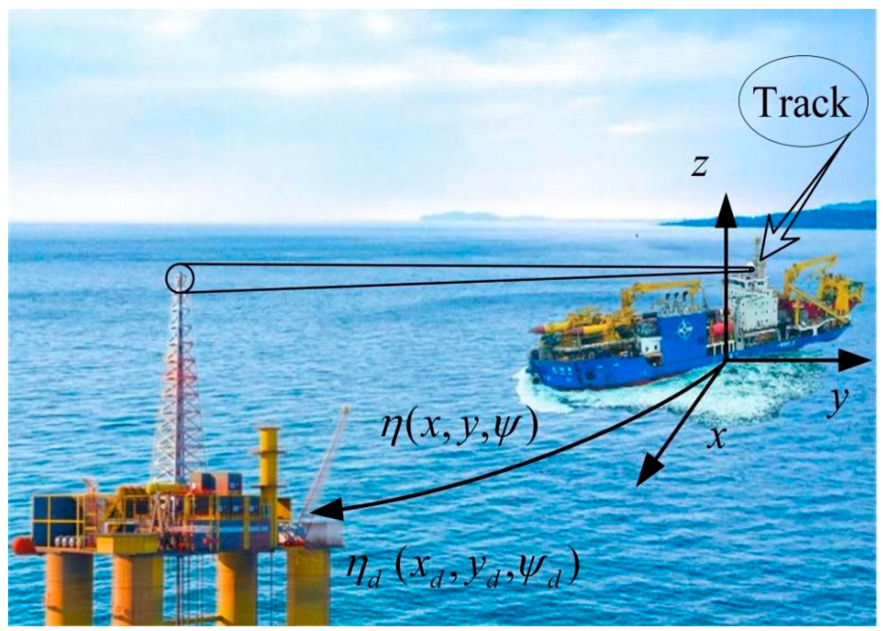
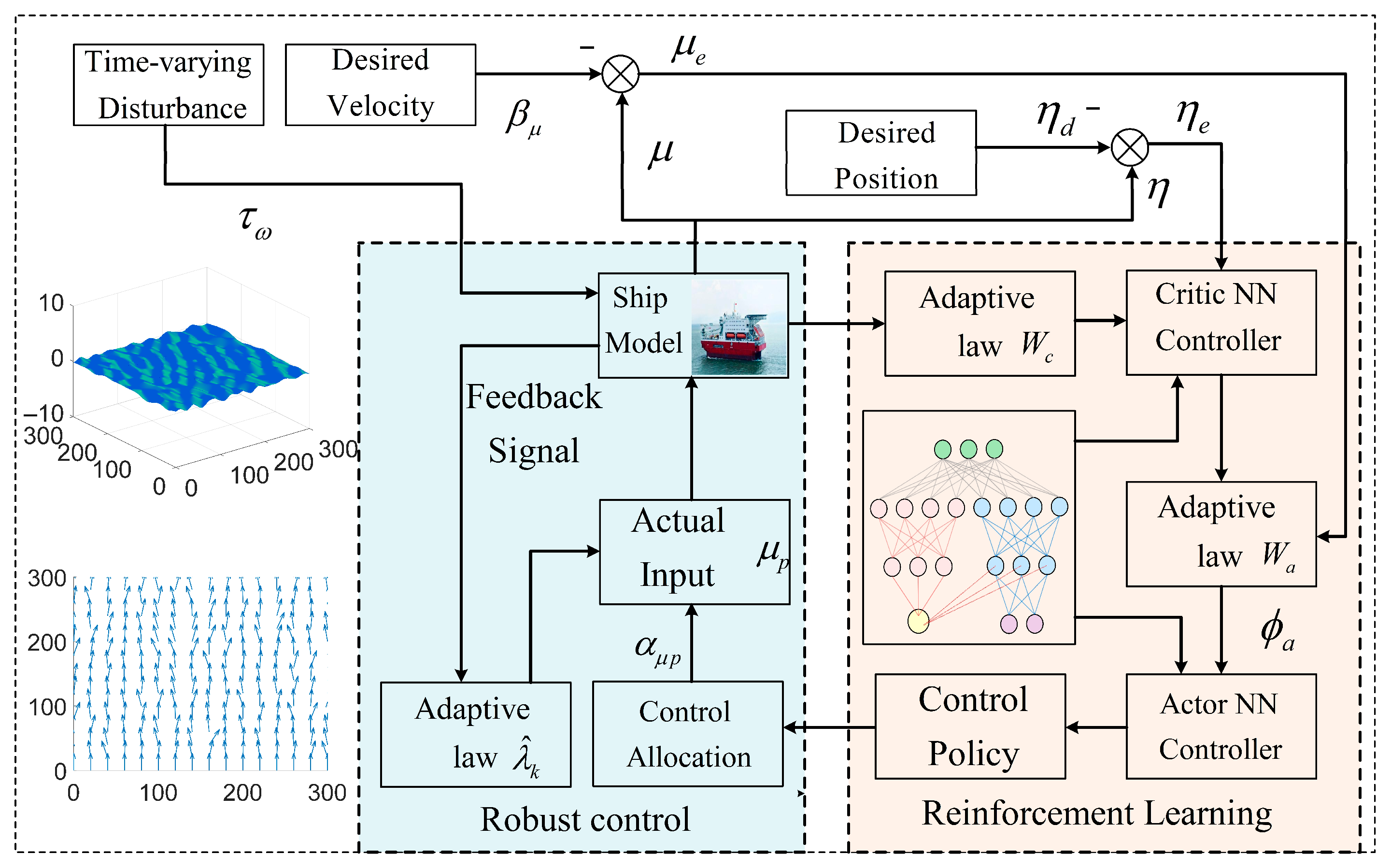
In this section, an RL approach based on the actor–critic framework is proposed to develop an adaptive control method [26] for the DP system of vessels. This method is capable of adapting to complex and dynamic marine environmental changes through continuous learning and the optimization of control policies. Under Assumptions 1 and 2, a robust neural adaptive control scheme is designed for the DP system, as described by Equations (1) and (2), utilizing dynamic surface control (DSC) techniques. The schematic diagram and detailed block diagram of the proposed DP system is illustrated in Figure 1 and Figure 2, providing a comprehensive overview of the system architecture.

Figure 1.
Schematic diagram of control effect of vessel DP system.
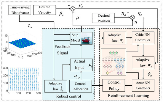
Figure 2.
Flowchart of the entire process of the vessel DP system based on reinforcement learning under time-varying interference.
3.1. Control Design
Let be the target position; the entire control synthesis consists of the following several steps. Define the position error vector as
Taking the time derivative of Equation (9), one has
Based on the position error dynamics Equation (10), the immediate control can be directly selected as
where is a positive definite diagonal matrix. Obviously, the differential expression of is very complicated and difficult to solve. In order to solve this problem, DSC technology [14,27] is applied, and the first-order filter is introduced in Equation (12) with the time constant matrix .
The vector as the output is the reference signal for the velocity vector . Meanwhile, ne can define the error vector as
and the velocity vector as
The derivative of is obtained by Equations (13) and (14)
where is a vector with its elements being bounded continuous functions. The position error derivative expression is further obtained from Equations (10) and (15) as
The primary control variable in the proposed design is chosen as Equation (22) for the desired thrusts term .
Due to system complexity and dynamic environmental/operational conditions, the servo system governing propeller thrust faces substantial uncertainties, which include load variations, environmental disturbances, and fluctuations in system parameters [25], inducing variations in the thrust coefficient and compromising the stability of the propulsion system [28]. To address these challenges, a robust adaptive control strategy is proposed for adjusting controller parameters in real time to adapt to changes in propeller dynamics or the vessel’s state [29]. The estimation of is accomplished using [30]. The control law, expressed as , is derived based on Equations (17) and (18), with the corresponding adaptive law detailed in Equation (19). This strategy ensures enhanced stability and operational efficiency under varying conditions.
where and are the positive parameters; especially, could protect the estimation from drifting divergence. denotes the pseudo inverse of . According to the adaptive law Equation (20), the gain correlation coefficient is added to compensate for the influence of model uncertainty and interference [31].
3.2. Critic and Actor NN Design
This section introduces the RL [32] utilizing the critic and actor method to control the DP of vessels [33,34]. At the same time, in order to construct the Bellman error of nonlinear systems, the long-term strategy performance index function [35] is defined as follows:
where is integral reinforcement interval, and is the discount rate that reduces the weight of this cost incurred further in the future. Based on the delay characteristics of the system, a smaller value (such as 0.9) was selected through the debugging of parameters in order to pay more attention to the long-term return. , which integrates future information that is not known at the current time related to the position error vector.
where denotes a small positive threshold associated with tracking accuracy, typically set as 0.2, and and express the parameters of and , respectively. Under the current control strategy, indicates a decrease in tracking performance and an increase in long-term performance indicators, while indicates the opposite, which reflects a significant tracking error under the current control strategy.
At the same time, the long-term strategy performance index function at time is defined as follows: , .
However, for the highly nonlinear and coupled system described in Equation (3), the long-term utility function incorporates future information that is unavailable at the current time, making it challenging to solve directly, even for linear systems. Only a limited class of nonlinear systems with specific functional designs and appropriate parameters can achieve the explicit evolution of . is particularly difficult to solve. To address this issue, the critic NN, which is utilized as the approximation, is expressed as where is the ideal weight matrix of the critic NN, is the input vector of the critic NN, and is the given critic NN vector. The actor NN operates based on the control law, driven by the critic NN’s evaluation of control performance [36].
From Equation (7), the actor NN is designed. The update mechanism aims to maintain closed-loop stability and optimize the performance index . However, since is unknown, and are utilized to approximate and in real time, respectively.
As outlined in [37], the strategic utility function is constructed as , where is the input vector of the actor NN system at time , represents the ideal weight matrix of the actor NN, and is an NN approximation error. Meanwhile, the temporal difference error is defined as , where . Positive constants , , , , , and exist such that , , , , , , , . Using a gradient descent algorithm, the adaptive control rate of critic and actor NN part are respectively defined as
where , are gain coefficients, , , , , and . By repeatedly adjusting the size of the gain coefficient in the simulation, the stability and convergence during the training process are guaranteed.
To prevent one network form dominating while the other stagnates, the mitigation of uncoordinated updates between actor and critic NN is solved by the inclusion of gain coefficients. and represent the self-defined learning rate matrix. Then, one can define the weight error as and . Neural networks play a crucial role in the training and performance of networks. To accelerate the training, adjust the network architecture to meet the requirements and ensure that in the actor–critic framework, the critic network can effectively estimate the value function, while the actor network can stably learn the optimal strategy.
Remark 1.
NNs are widely recognized as effective tools for the adaptive approximation of complex unknowns, such as unmodeled dynamics and uncertainties, within intelligent learning-based control frameworks. RL techniques, particularly those employing actor–critic architectures, are designed to optimize long-term rewards through a continuous interaction with online control performance. This performance is inherently influenced by both internal control strategies and external disturbances, which collectively shape the system’s behavior and adaptability. Through multiple repeated experiments, the parameters are evaluated, and the balance of each parameter is adjusted. Due to the complex design of the dynamic adjustment strategy, the hyperparameters need to be adjusted multiple times. Relying on empirical adjustment and repeated trial and error, the values of the parameters are finally determined in Equation (39).
3.3. Stability Analysis
Theorem 1.
Consider a closed-loop system composed of vessel dynamics, a robust neural control law, an actor–critic NN, and adaptive laws. Assume that the initial conditions are satisfied:
and there exist adjustable parameters . Then, the closed-loop system consisting of the vessel model Equations (1) and (2), the control law Equations (11) and (20), and the adaptive law Equation (19) is stable. The proposed adaptive NN controller, integrating RL, ensures the following closed-loop properties for all initial conditions:
- (1)
- Semi-Global Uniform Ultimate Boundedness: The state variables of the closed-loop system are semi-globally uniformly ultimately bounded;
- (2)
- Tightly Concentrated Errors: The tracking position error , tracking velocity error , and the NN weight errors and are kept within a tight region;
- (3)
- The optimal control strategy in RL is determined by approximating the ideal unknown weights. An estimator of actor and critic weights is designed to allow the NN to update recursively in parallel.
The proof is as follows: According to the characteristics of vessel DP and control design, the following Lyapunov function is used:
The time derivative of Equation (25) is
Similar to the former, we further have
According to Equations (4) and (14) and Young’s inequality,
where the term is treated with an approximation. And according to Equation (28),
Moreover, we also have
Through the designed adaptive control law, Equation (19) is further obtained by
The first term cancels out the one of , and the second term is determined by Young’s inequality:
Finally, according to Equation (24), the error of RL weight is analyzed as
To sum up, the final form is obtained by combining from Equation (27) to Equation (34):
The design parameters are appropriately selected, satisfying
where
By adjusting the following parameter matrix, all tracking errors of the closed-loop control system are converged to a compact set. Further, by adjusting the parameter , the following conditions can be obtained. Integrating two sides of Equation (35), one can obtain . The can converge into with , and the bounded variable can be small enough through turning the control parameters appropriately. Therefore, all the state variables in the closed-loop control system are SGUUB.
4. Numerical Simulation
In this section, two representative case studies are compared to illustrate the effectiveness and merits of the control scheme, i.e., a comparative experiment with the result in [38], and in order to verify the DP adaptive control method based on integral RL, MATLAB 2024a is used as the simulation platform to conduct experiments on the marine environment model. The DP system model used in the experiment includes a thruster, servo system, control system, and external disturbance model. And the environmental disturbances are as follows: the wind is at level 6, the number of wave frequency segments is 10, and the wave velocity is . The nominal physical parameters [39] of the vessels are as follows in Equation (38):
With the initial states and , the desired position and heading are chosen as . The design parameters utilized for the model are chosen as in Equation (39):
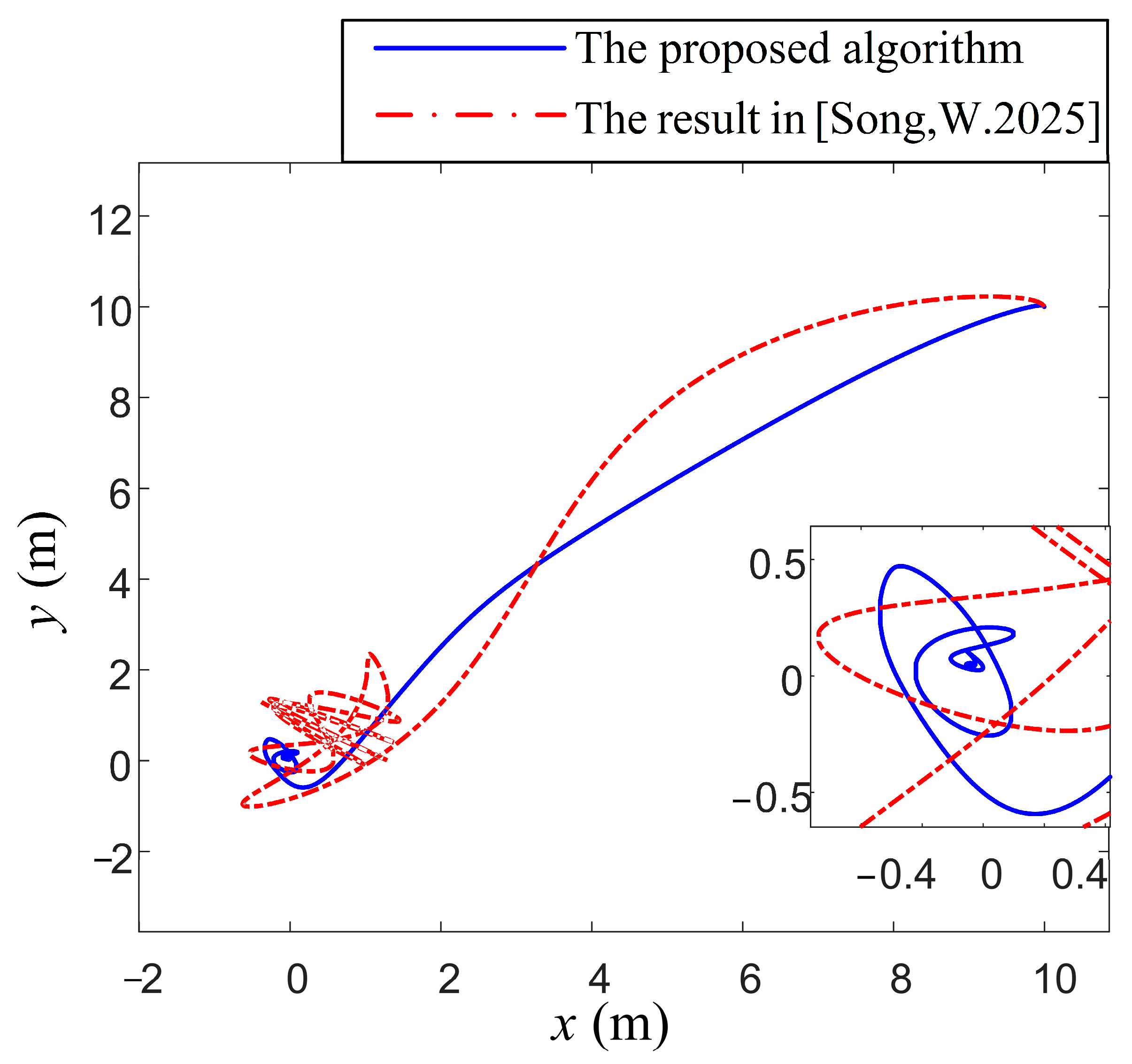
The comparative experimental results are illustrated in Figure 3, Figure 4, Figure 5 and Figure 6. In Figure 3, with its trajectory exhibiting a narrower error range and smoother curve, the vessel’s position ultimately stabilizes within the desired attitude domain. As the simulation progresses, the system demonstrates a high accuracy, with the proposed algorithm outperforming in terms of control and positioning precision. The trajectory (the proposed curve) converges tightly within the desired error boundary. In contrast, the other curve shows persistent oscillations with a maximum deviation.

Figure 3.
Comparison of position control performance under different algorithms [38].
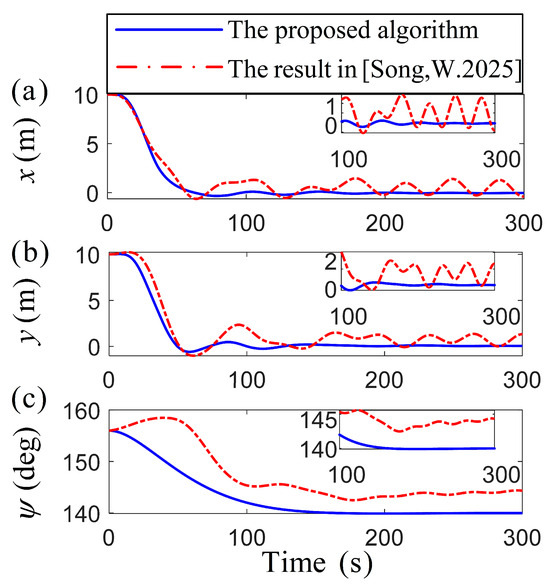
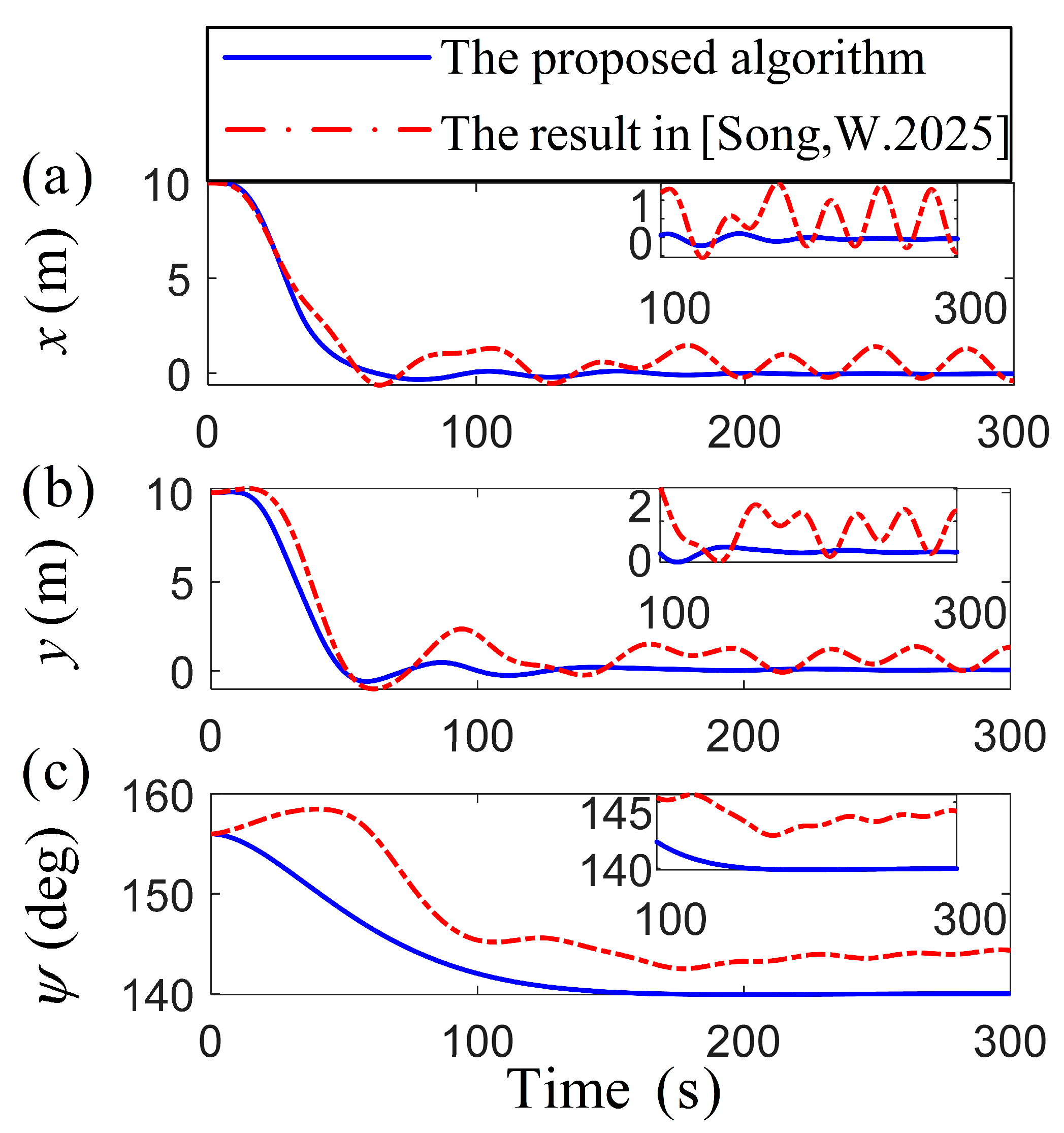
Figure 4.
Comparison of the vessel position vector variables [38].

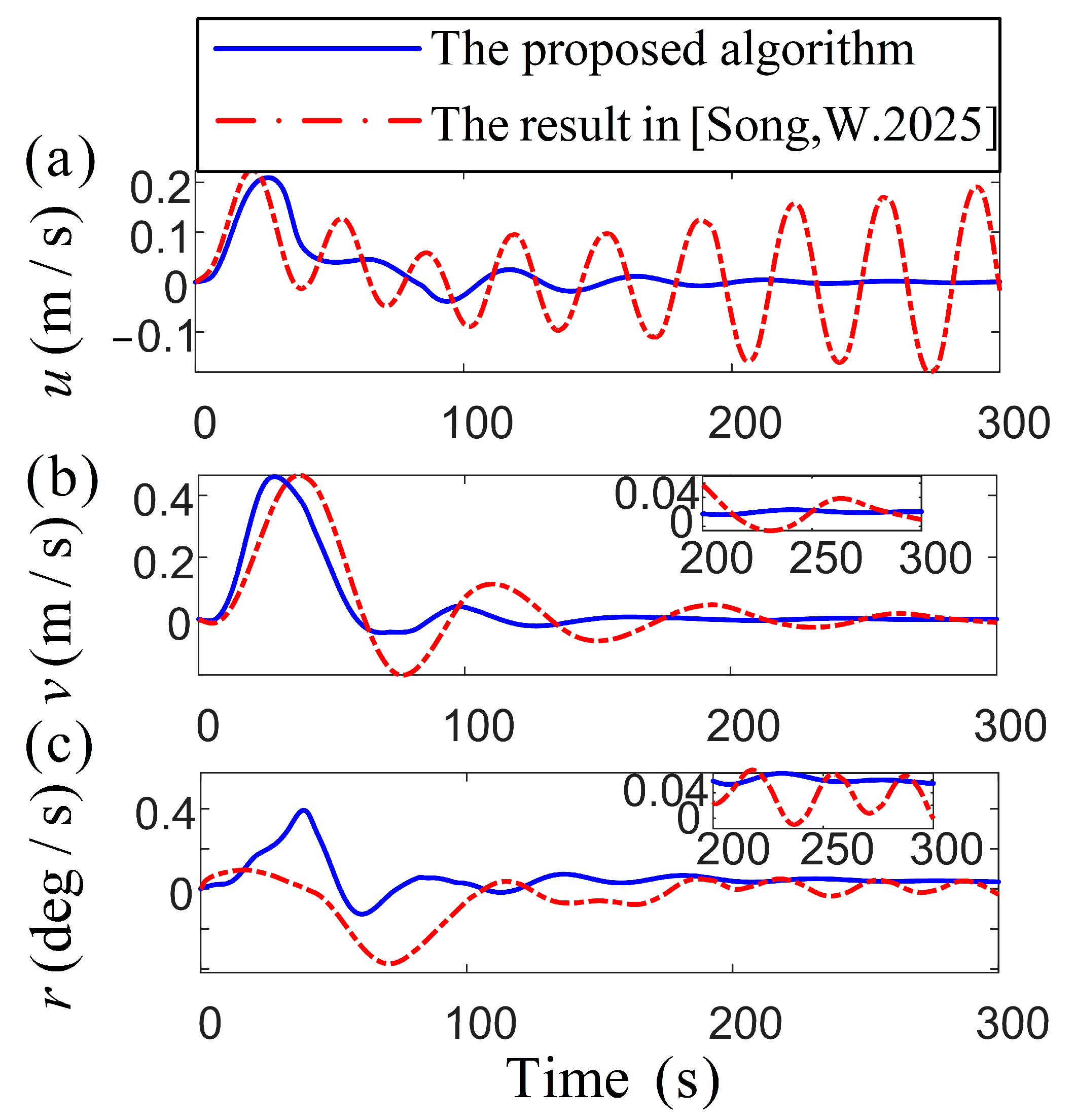
Figure 5.
Comparison of the vessel velocity vector variables [38].
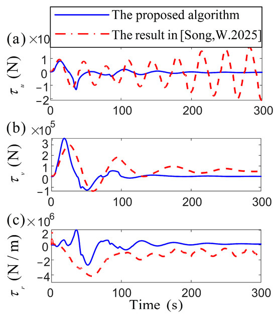
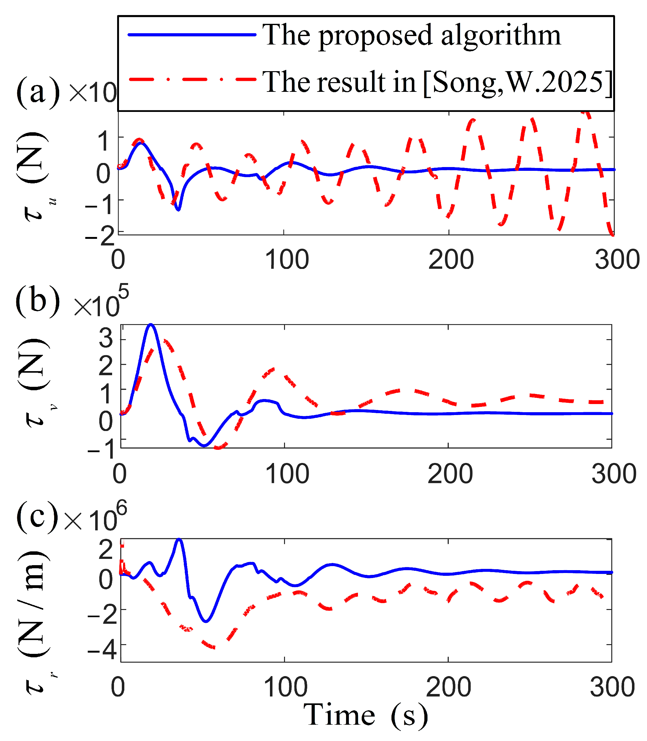
Figure 6.
Comparison of the vessel control inputs [38].
The comparison of specific position parameters in Figure 4 reveals that both algorithms attain fast convergence within the target region. However, the algorithm from [38], exhibits significant fluctuations in attitude and velocity errors, whereas the proposed algorithm maintains smoother variations, achieving a precise targeting of the desired attitude. Figure 5 presents a remarkable demonstration of control robustness, with the proposed algorithm reducing speed variations by an order of magnitude compared to the oscillatory behavior characteristic of conventional methods [38]. Under substantial external disturbances, the proposed algorithm reduces the speed fluctuations of the vessel to the target point more stably. Based on the adaptive control algorithm’s ability, the outcome highlights the RL optimizing the system’s response to disturbance, reducing the necessity for abrupt adjustments in propeller output to accommodate environmental changes. During the initial stage, there is a significant transient overshoot in [38], while the proposed algorithm has an overshoot of no more than 0.1 . Safety improvement: The steady-state fluctuation range of and is reduced, indicating that the vessel is less susceptible to drift caused by wind and waves during positioning operations. Its low fluctuation and high-precision characteristics are particularly suitable for high-demand marine engineering scenarios. In the comparison in Figure 6, the proposed algorithm demonstrates smoother temporal variations in force and torque, minimizing sudden adjustments or fluctuations in control inputs. For DP systems requiring high precision and stability, the proposed method significantly enhances operational stability and control efficiency, thereby improving overall system performance metrics. The attenuation rate determines the speed at which the system state tends to be stable. It can be seen from the theoretical analysis that the convergence effect is good. In Figure 3 and Figure 4, both the velocity vector and the position vector have converged to zero in the domain near 100 s, and the dynamic indicators such as the overshoot and the adjustment time perform well. RL and adaptive control methods are adopted to further improve the convergence speed and enhance the transient response characteristics of the system. This scheme ensures that the system reaches a stable process quickly and smoothly, reduces over-rush and slows oscillation to make the oscillation amplitude smaller, and improves the stability of the system.
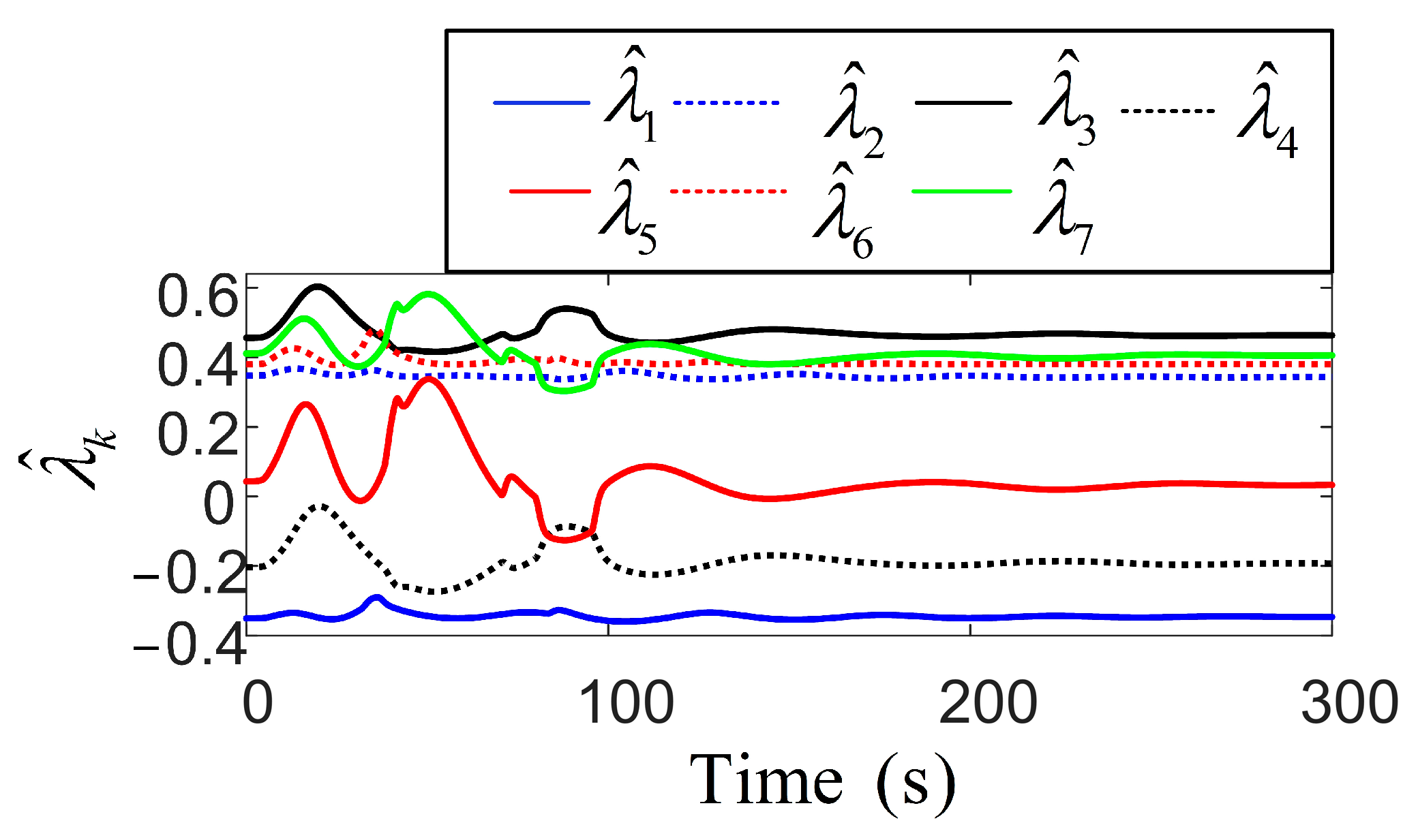
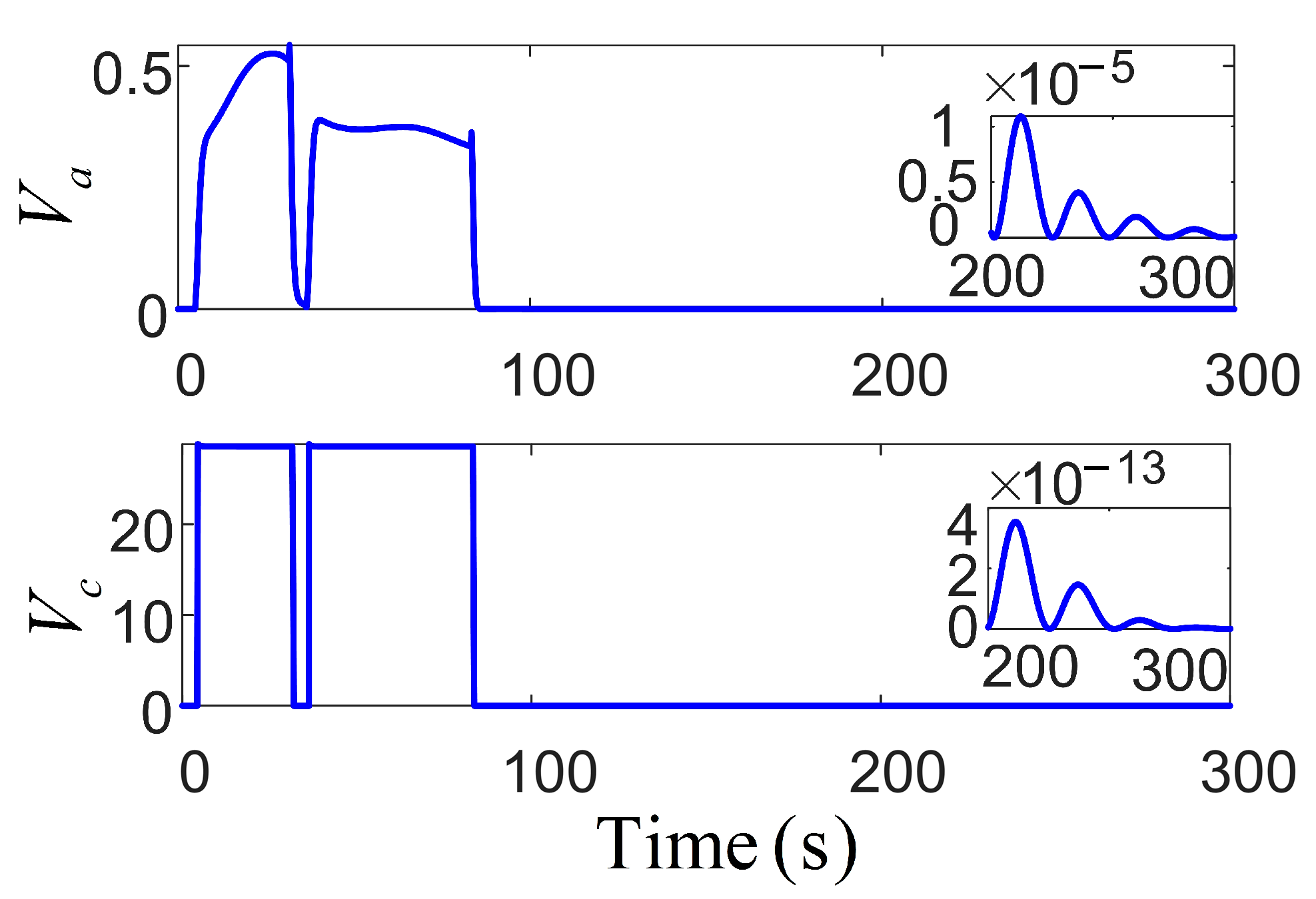
Figure 7 depicts the pitch rate of the control propeller, in the simulation experiments, with all values falling within reasonable ranges. The two subplots represent the pitch ratio and the azimuth angle of the azimuth thruster, respectively [30]. The azimuth angle of the propeller directly affects the anti-drift ability of the vessel by controlling the thrust direction of the thruster. Its dynamic adjustment can align the thrust vector in reverse with environmental disturbances (such as wind loads), significantly enhancing the positioning stability. Multiple thrusters are combined through differentiated azimuth angles to form a cooperative thrust vector field, achieving high-precision torque control. This azimuth–pitch joint control mechanism is optimized in real time through an adaptive algorithm. It can not only adjust the thrust phase in advance, according to the environmental interference prediction model, to avoid overdraft but also dynamically reconstruct the thrust distribution when the thruster fails. Figure 8 illustrates significant variations in the long-term utility function. Over time, the control system progressively minimizes the heading angle error, rendering changes negligible over time, thus achieving the required performance and stability. The primary objective of both networks is to minimize the utility function, optimizing the control strategy and reducing the impact of wind and wave variations to ensure high-precision positioning.
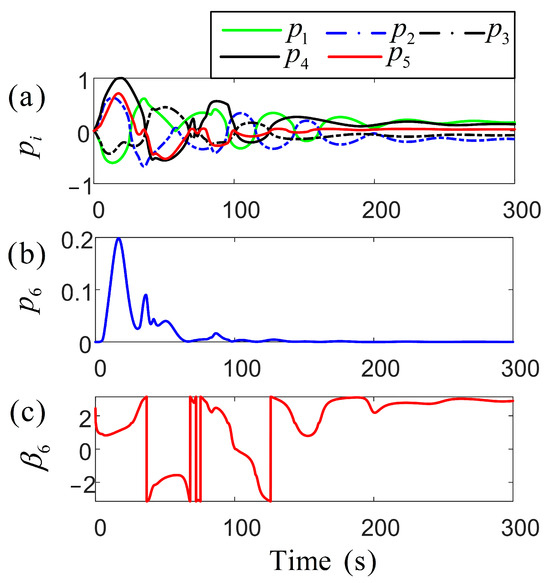
Figure 7.
Schematic diagram of the timing sequence for adjusting the pitch and azimuth angles of the propeller during the analysis of the parameter response of the thruster and the steady-state performance .
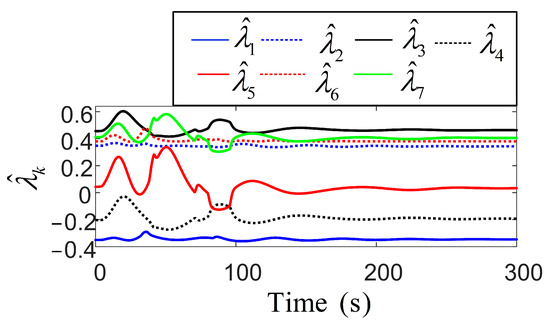
Figure 8.
The adaptive parameter dynamic adjustment analysis diagram under the proposed algorithm.
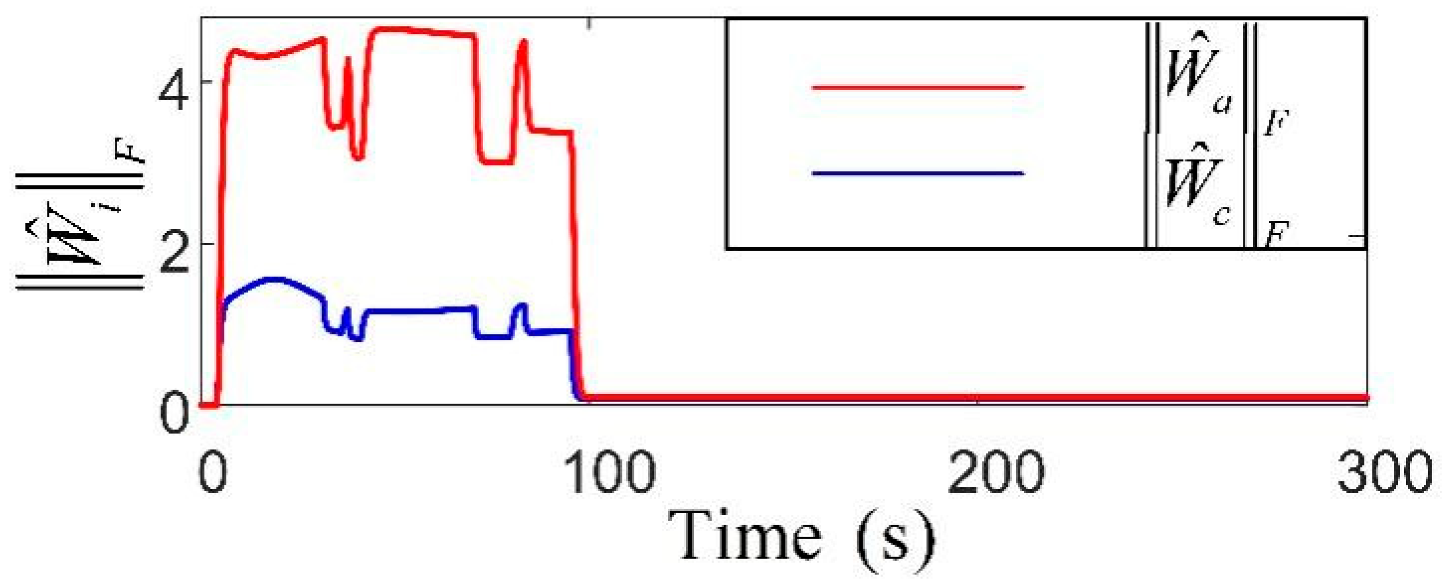
Figure 9 presents the parameters of the robust adaptive control, where the incorporation of the RL network significantly smooths their fluctuations, reflecting improved control performance. Subsequently, both position and velocity vector fluctuations remain minimal, maintaining precise positioning and robustness against disturbances in complex environments. Notably, due to the larger parameter space required for policy learning, the weight norm of the actor network is slightly larger than that of the critic network, reflecting its higher structural complexity. In contrast, the critic, which estimates the value function, typically operates within a less complex action space, leading to a smaller weight norm. This observation underscores the distinct structural and training demands of the two networks during the learning process. Figure 10 and Figure 11 present the cost function trends and norm of the current weights for the two networks. With more fluctuations in the early learning phase, the critics cost quantifies the error in estimating the long-term utility. The norm of the actor weights updates and focuses on optimizing the strategy to enhance future expected rewards, showing greater variation due to uncertainty in the training environment. The primary objective of the actor–critic RL method in tuning the action–critic NNs is to minimize the cost function and , effectively tracking the target heading and maintaining small heading errors despite environmental disturbances. This method dynamically adjusts the control strategy based on historical data and environmental feedback, demonstrating a high accuracy in practical applications. The critic network evaluates the long-term value function and directs the actor to focus on actions that minimize cumulative future errors. The actor network learns a strategy that achieves a balance between tracking accuracy and energy efficiency. The proposed RL framework ensures adaptability to non-stationary disturbances, while avoiding the excessive punishment of control efforts. It is achieved through collaborative actor-driven strategy optimization and critic-guided value learning.

Figure 9.
Long-term effect strategy function time evolution analysis.
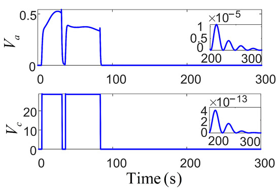
Figure 10.
The variation in the cost function based on actor–critic RL.

Figure 11.
Adaptive weight matrix norm variation curve based on actor–critic framework.
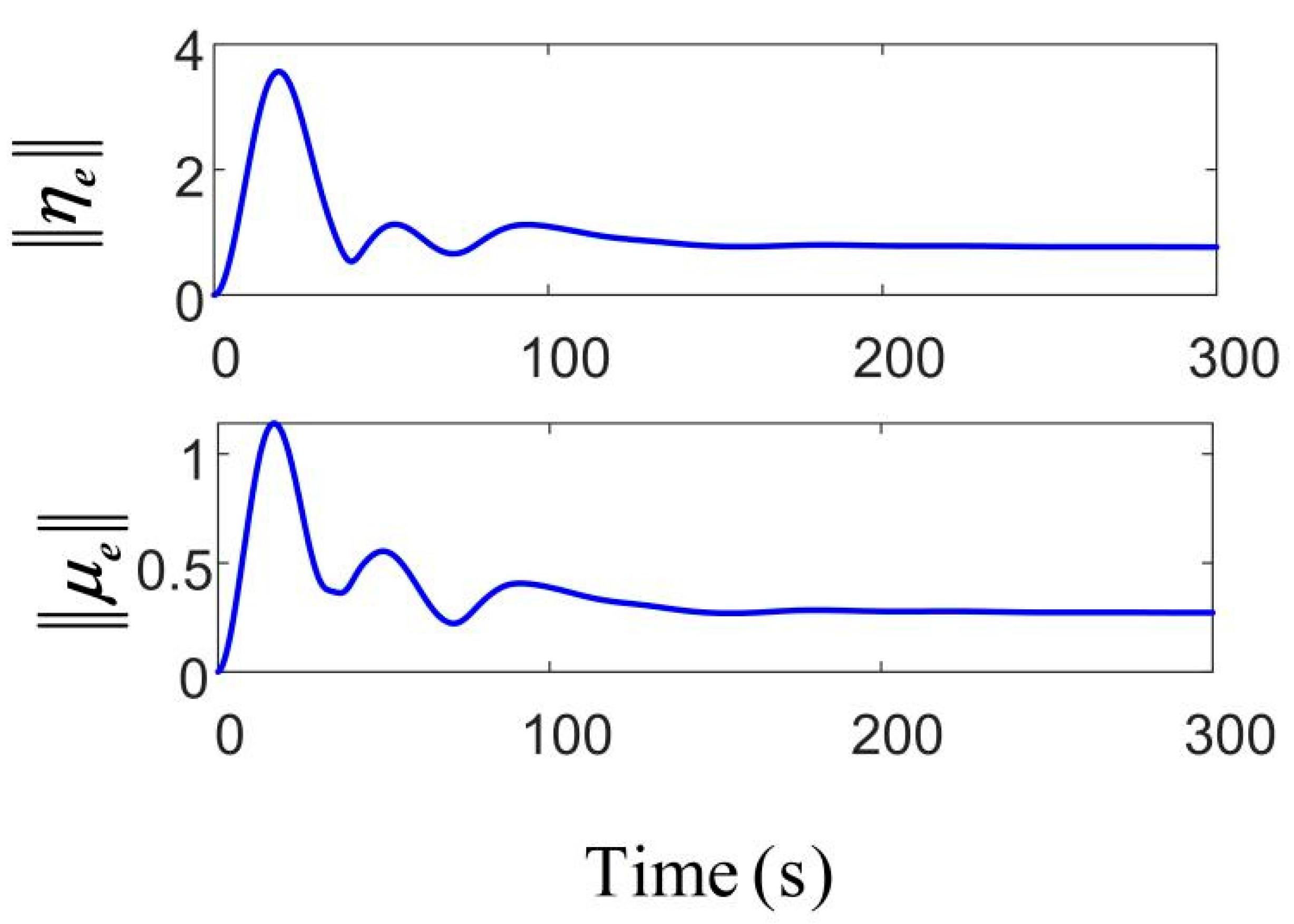
In Figure 12, in the area where the position and velocity error values rapidly decrease and then return to zero, even when the system is confronted with disturbances under harsh sea conditions, it can still rapidly converge and maintain stability and robustness.

Figure 12.
Norm of the position and velocity errors.
Through the RL process, the agent learns the most energy-efficient control strategy while maintaining control precision, particularly in unstable sea conditions, where the system optimally manages propeller operations to avoid excessive adjustments. It could be heavily impacted by harsh sea conditions in [38], and its capacity to mitigate such disturbances was relatively weak. In contrast, the single parameter of the proposed algorithm can be finely adjusted, enabling the gradual stabilization of the critic network’s value estimation. With adequate training and sufficient interaction with the environment, the algorithm demonstrates improved performance.
5. Conclusions
Even though robust adaptive control boasts strong stability and the ability to handle uncertainties, when facing extreme conditions, especially sea condition changing rapidly, its judgement is slow, and its energy consumption is high. By combining RL with traditional robust control, it performs well in dynamic maritime environments, significantly reducing position and heading errors, while optimizing energy efficiency and ensuring real-time adaptability, which guarantees smaller error fluctuations and enhanced stability. Moreover, it addresses the problems of response delay and performance degradation in extreme conditions. This synergy improves control accuracy and stability, making it highly effective in challenging maritime operations.
Author Contributions
Conceptualization, J.L., W.H. and C.H.; methodology, W.H.; software, W.H.; validation, J.L. and C.H.; formal analysis, J.L.; investigation, J.L.; writing—original draft preparation, W.H.; writing—review and editing, J.L. and G.Z.; supervision, J.L.; project administration, G.Z.; funding acquisition, J.L. All authors have read and agreed to the published version of the manuscript.
Funding
The paper is partially supported by the National Excellent Youth Science Fund of China (52322111), the National Natural Science Foundation of China (52171291), the Dalian Science and Technology Program for Distinguished Young Scholars (2022RJ07), and the Fundamental Research Funds for the Central Universities (3132023137, 3132023502). The authors would like to thank the anonymous reviewers for their valuable comments.
Data Availability Statement
The original contributions presented in this study are included in the article. Further inquiries can be directed to the corresponding author.
Conflicts of Interest
The authors declare no conflicts of interest.
References
- Zhai, M.; Wu, W.; Tsai, S. The Effects of Artificial Intelligence Orientation on Inefficient Investment: Firm-Level Evidence from China’s Energy Enterprises. Energy Econ. 2025, 141, 108048. [Google Scholar] [CrossRef]
- Alagili, O.; Fernando, E.; Ahmed, S.; Imtiaz, S.; Murrant, K.; Gash, B.; Islam, M.; Zaman, H. Experimental Investigations of An Energy-Efficient Dynamic Positioning Controller for Different Sea Conditions. Ocean Eng. 2024, 299, 117297. [Google Scholar] [CrossRef]
- Xie, W.; Liang, J.; Wang, Z.; Yang, J. Non-Monotonic Lyapunov Function Based Membership Function Dependent Robust Control of Takagi-Sugeno Fuzzy Systems. Eng. Appl. Artif. Intell. 2025, 152, 110785. [Google Scholar] [CrossRef]
- Hatami, E.; Salarieh, H. Adaptive Critic-Based Neuro-Fuzzy Controller for Dynamic Position of Ships. Sci. Iran. 2015, 22, 272–280. [Google Scholar]
- Wan, L.; Fu, L.; Li, C.; Li, K. Flexible Job Shop Scheduling via Deep Reinforcement Learning with Meta-Path-Based Heterogeneous Graph Neural Network. Knowl.-Based Syst. 2024, 296, 111940. [Google Scholar] [CrossRef]
- Wang, D.; Zhao, H.; Zhang, L.; Chen, K. Learning to Dispatch for Flexible Job Shop Scheduling Based on Deep Reinforcement Learning via Graph Gated Channel Transformation. IEEE Access 2024, 12, 50935–50948. [Google Scholar]
- Zhao, L.; Bai, Y. Unlocking the Ocean 6G: A Review of Path-Planning Techniques for Maritime Data Harvesting Assisted by Autonomous Marine Vehicles. J. Mar. Sci. Eng. 2024, 12, 126. [Google Scholar] [CrossRef]
- Liu, Z.; Zhang, O.; Gao, Y.; Zhao, Y.; Sun, Y.; Liu, J. Adaptive Neural Network-Based Fixed-Time Control for Trajectory Tracking of Robotic Systems. IEEE Trans. Circuits Syst. II Express Briefs 2023, 70, 241–245. [Google Scholar] [CrossRef]
- Li, J.; Zhang, G.; Cabecinhas, D.; Pascoal, A.; Zhang, W. Prescribed Performance Path Following Control of USVs via An Output-Based Threshold Rule. IEEE Trans. Veh. Technol. 2024, 73, 6171–6182. [Google Scholar] [CrossRef]
- Ma, D.; Chen, X.; Ma, W.; Zheng, H.; Qu, F. Neural network Model Based Reinforcement Learning Control for AUV 3-D Path Following. IEEE Trans. Intell. Veh. 2014, 9, 893–904. [Google Scholar] [CrossRef]
- Li, J.; Zhang, G.; Zhang, X.; Zhang, W. Integrating Dynamic Event-Triggered and Sensor-Tolerant Control: Application to USV-UAVs Cooperative Formation System for Maritime Parallel Search. IEEE Trans. Intell. Transp. Syst. 2025, 25, 3986–3998. [Google Scholar] [CrossRef]
- Wang, Y.; Bai, W.; Zhang, W.; Chen, S.; Zhao, Y. Optimal Course Tracking Control of USV with Input Dead Zone Based on Adaptive Fuzzy Dynamic Programing. Proc. Inst. Mech. Eng. Part J. Syst. Control Eng. 2024. [CrossRef]
- Zhang, G.; Sun, Z.; Li, J.; Huang, J.; Bin, Q. Iterative Learning Control for Path-following of ASV with the Ice Floes Auto-select Avoidance Mechanism. IEEE Trans. Intell. Transp. Syst. 2025; early access. [Google Scholar] [CrossRef]
- Qu, C.; Cheng, L.; Ga Gao, S.; Huang, X. Experience Replay Enhances Excitation Condition of Neural-Network Adaptive Control Learning. J. Guid. Control Dyn. 2025, 48, 496–507. [Google Scholar] [CrossRef]
- Ning, J.; Ma, Y.; Chen, C. Event-Triggered-Based Distributed Formation Cooperative Tracking Control of Under-Actuated Unmanned Surface Vehicles with Input and State Quantization. IEEE Trans. Intell. Transp. Syst. 2025, 26, 7081–7097. [Google Scholar] [CrossRef]
- Gao, Y.; Su, S.; Zong, Y.; Zhang, L.; Guo, X. Adaptive Fuzzy Gain-Scheduling Robust Control for Stability of Quadrotors. Appl. Math. Model. 2025, 138, 115816. [Google Scholar] [CrossRef]
- He, Y.; Liu, Y.; Yang, L.; Qu, X. Deep Adaptive Control: Deep Reinforcement Learning-Based Adaptive Vehicle Trajectory Control Algorithms for Different Risk Levels. IEEE Trans. Intell. Veh. 2024, 9, 1654–1666. [Google Scholar] [CrossRef]
- Wang, S.; Li, J.; Jiao, Q.; Ma, F. Design Patterns of Deep Reinforcement Learning Models for Job Shop Scheduling Problems. J. Intell. Manuf. 2024. [CrossRef]
- Yang, Y.; Geng, S.; Yue, D.; Gorbachev, S.; Korovin, I. Event-Triggered Approximately Optimized Formation Control of Multi-Agent Systems with Unknown Disturbances via Simplified Reinforcement Learning. Appl. Math. Comput. 2025, 489, 129149. [Google Scholar] [CrossRef]
- Abreu, M.; Reis, L.; Lau, N. Addressing Imperfect Symmetry: A Novel Symmetry-Learning Actor-Critic Extension. Neurocomputing 2025, 614, 128771. [Google Scholar] [CrossRef]
- Tagliaferri, F.; Viola, I. A Real-Time Strategy Decision Program for Sailing Yacht Races. Ocean Eng. 2017, 134, 129–139. [Google Scholar] [CrossRef]
- Ning, J.; Wang, Y.; Chen, C.; Li, T. Neural Network Observer Based Adaptive Trajectory Tracking Control Strategy of Unmanned Surface Vehicle with Event-Triggered Mechanisms and Signal Quantization. IEEE Trans. Emerg. Top. Comput. Intell. 2025; early access. [Google Scholar] [CrossRef]
- Zhang, G.; Yin, S.; Li, J.; Zhang, W.; Zhang, W. Game-Based Event-Triggered Control for Unmanned Surface Vehicle: Algorithm Design and Harbor Experiment. IEEE Trans. Cybern. 2025; early access. [Google Scholar] [CrossRef]
- He, W.; Dong, Y.; Sun, C. Adaptive Neural Impedance Control of a Robotic Manipulator with Input Saturation. IEEE Trans. Syst. Man Cybern. Syst. 2016, 46, 334–344. [Google Scholar] [CrossRef]
- Liu, Z.; Zhao, Y.; Zhang, O.; Chen, W.; Wang, J.; Gao, Y.; Liu, J. A Novel Faster Fixed-Time Adaptive Control for Robotic Systems with Input Saturation. IEEE Trans. Ind. Electron. 2024, 71, 5215–5223. [Google Scholar] [CrossRef]
- Shen, H.; Wu, J.; Wang, Y.; Wang, J. Reinforcement Learning-Based Robust Tracking Control for Unknown Markov Jump Systems and Its Application. IEEE Trans. Circuits Syst. II-Express Briefs 2024, 71, 1211–1215. [Google Scholar] [CrossRef]
- Li, H.; Zhang, T. Neural Adaptive Dynamic Event-Triggered Practical Fixed-Time Dynamic Surface Control for Non-Strict Feedback Nonlinear Systems. Int. J. Adapt. Control Signal Process. 2022, 36, 3066–3086. [Google Scholar] [CrossRef]
- Liu, A.; Wang, D.; Qiao, J. An Advanced Robust Integral Reinforcement Learning Scheme with The Fuzzy Inference System. Int. J. Robust Nonlinear Control 2024, 34, 11745–11759. [Google Scholar] [CrossRef]
- Chen, Y.; Ding, J.; Chen, Y.; Yan, D. Nonlinear Robust Adaptive Control of Universal Manipulators Based on Desired Trajectory. Appl. Sci. 2024, 15, 2219. [Google Scholar] [CrossRef]
- Chwa, D. Tracking Control of Differential Drive Wheeled Mobile Robots Using a Backstepping Like Feedback Linearization. IEEE Trans. Syst. Man Cybern. Part A-Syst. Hum. 2010, 40, 1285–1295. [Google Scholar] [CrossRef]
- Zhang, G.; Cai, Y.; Zhang, W. Robust Neural Control for Dynamic Positioning Ships with The Optimum-Seeking Guidance. IEEE Trans. Syst. Man Cybern. Syst. 2017, 47, 1500–1509. [Google Scholar] [CrossRef]
- Zheng, L.; Fiez, T.; Alumbaugh, Z.; Chasnov, B.; Ratliff, L. Stackelberg Actor-Critic: Game-Theoretic Reinforcement Learning Algorithms. IEEE Trans. Neural Netw. Learn. Syst. 2022, 36, 9217–9224. [Google Scholar] [CrossRef]
- Zhang, G.; Li, Z.; Li, J.; Zhang, W.; Bin, Q. Prescribed Performance Path Following Control for Rotor-Assisted Vehicles via an Improved Reinforcement Learning Mechanism. IEEE Trans. Neural Netw. Learn. Syst. 2025; early access. [Google Scholar] [CrossRef]
- Xu, B.; Yang, C.; Shi, Z. Reinforcement Learning Output Feedback NN Control Using Deterministic Learning Technique. IEEE Trans. N Neural Netw. Learn. Syst. 2014, 25, 635–641. [Google Scholar]
- Qin, C.; Zhu, T.; Jiang, K.; Wu, Y. Integral Reinforcement Learning-Based Dynamic Event-Triggered Safety Control for Multiplayer Stackelberg-Nash Games with Time-Varying State Constraints. Eng. Appl. Artif. Intell. 2024, 133, 108317. [Google Scholar] [CrossRef]
- Zheng, Z.; Ruan, L.; Zhu, M.; Guo, X. Reinforcement Learning Control for Underactuated Surface Vessel with Output Error Constraints and Uncertainties. IEEE Trans. Veh. Technol. 2020, 399, 479–490. [Google Scholar] [CrossRef]
- Hou, Y.; Lin, M.; Anjidani, M.; Nik, H. Robust Optimal Control of Point-Feet Biped Robots Using a Reinforcement Learning Approach. IETE J. Res. 2024, 70, 7831–7846. [Google Scholar] [CrossRef]
- Song, W.; Zuo, Y.; Tong, S. Fuzzy Optimal Event-Triggered Control for Dynamic Positioning of Unmanned Surface Vehicle. IEEE Trans. Syst. Man Cybern.-Syst. 2025, 55, 2302–2311. [Google Scholar] [CrossRef]
- Zhang, G.; Xing, Y.; Zhang, W.; Li, J. Prescribed Performance Control for USV-UAV via a Robust Bounded Compensating Technique. IEEE Trans. Control. Netw. Syst. 2025; early access. [Google Scholar] [CrossRef]


Disclaimer/Publisher’s Note: The statements, opinions and data contained in all publications are solely those of the individual author(s) and contributor(s) and not of MDPI and/or the editor(s). MDPI and/or the editor(s) disclaim responsibility for any injury to people or property resulting from any ideas, methods, instructions or products referred to in the content. |
© 2025 by the authors. Licensee MDPI, Basel, Switzerland. This article is an open access article distributed under the terms and conditions of the Creative Commons Attribution (CC BY) license (https://creativecommons.org/licenses/by/4.0/).