

The Prediction of the Valve Opening Required for Slugging Control in Offshore Pipeline Risers Based on Empirical Closures and Valve Characteristics


Abstract
1. Introduction
2. Experiment
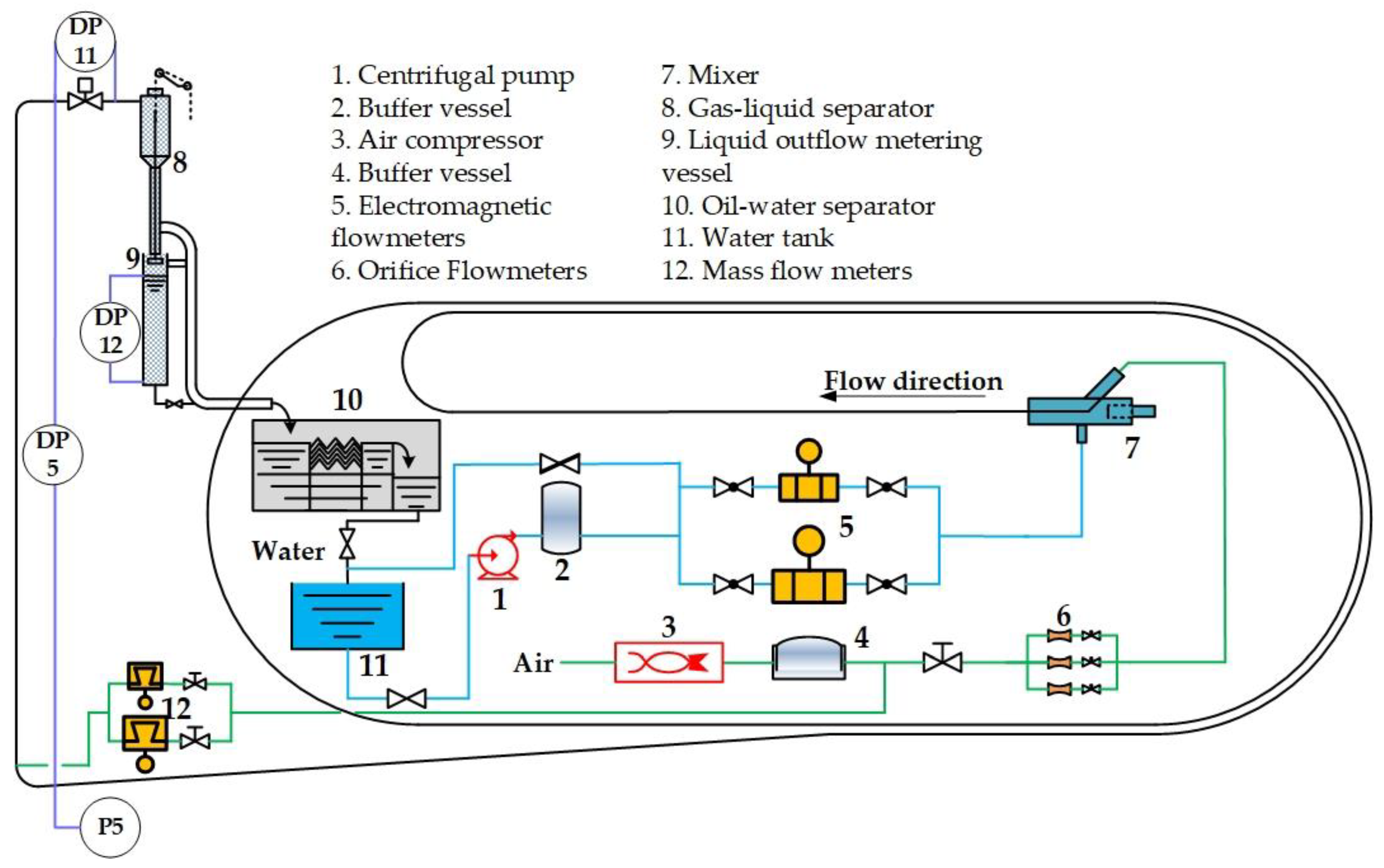
2.1. Setup of Experimental Loop
2.2. Experimental Condition
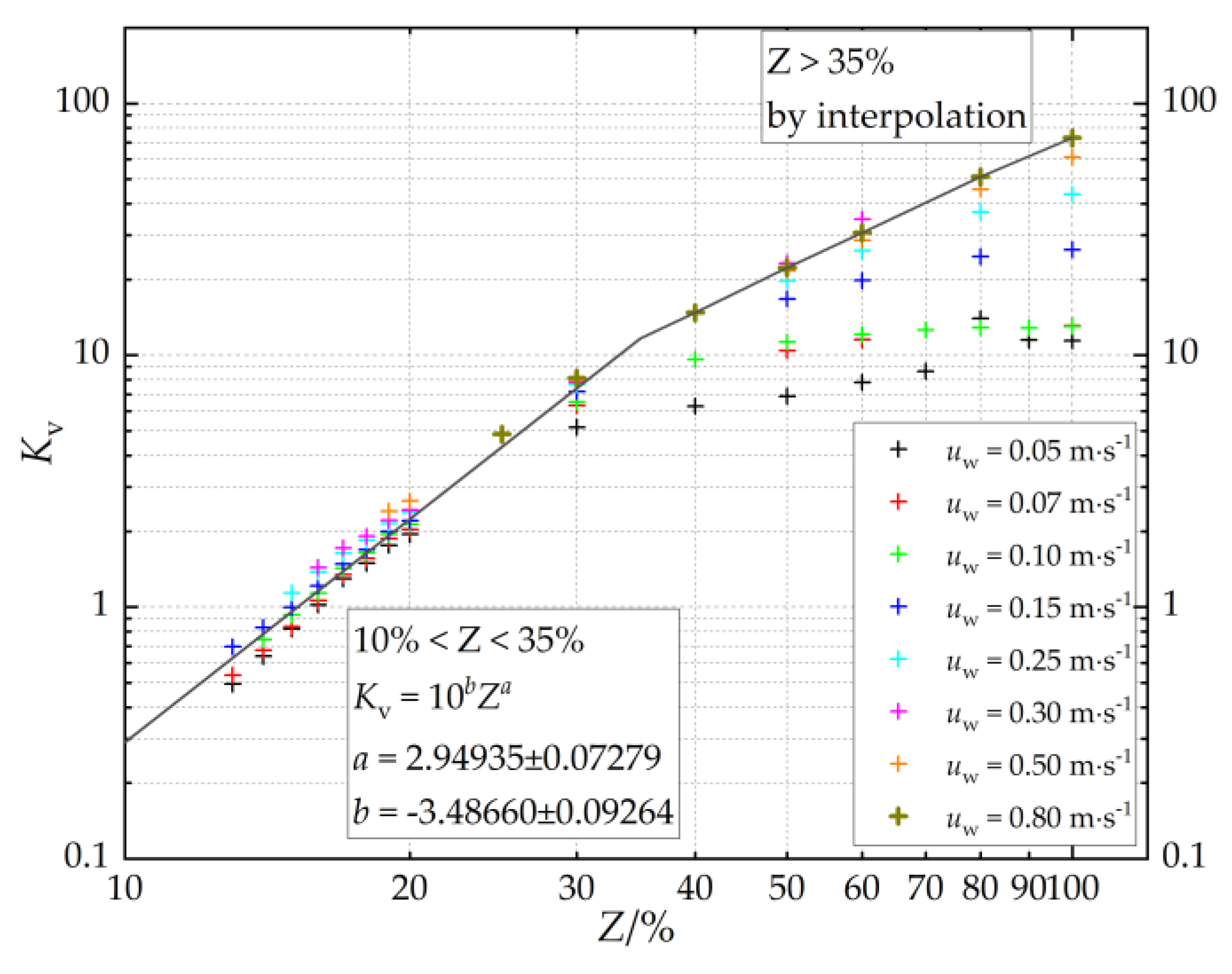
2.3. Flow Coefficient
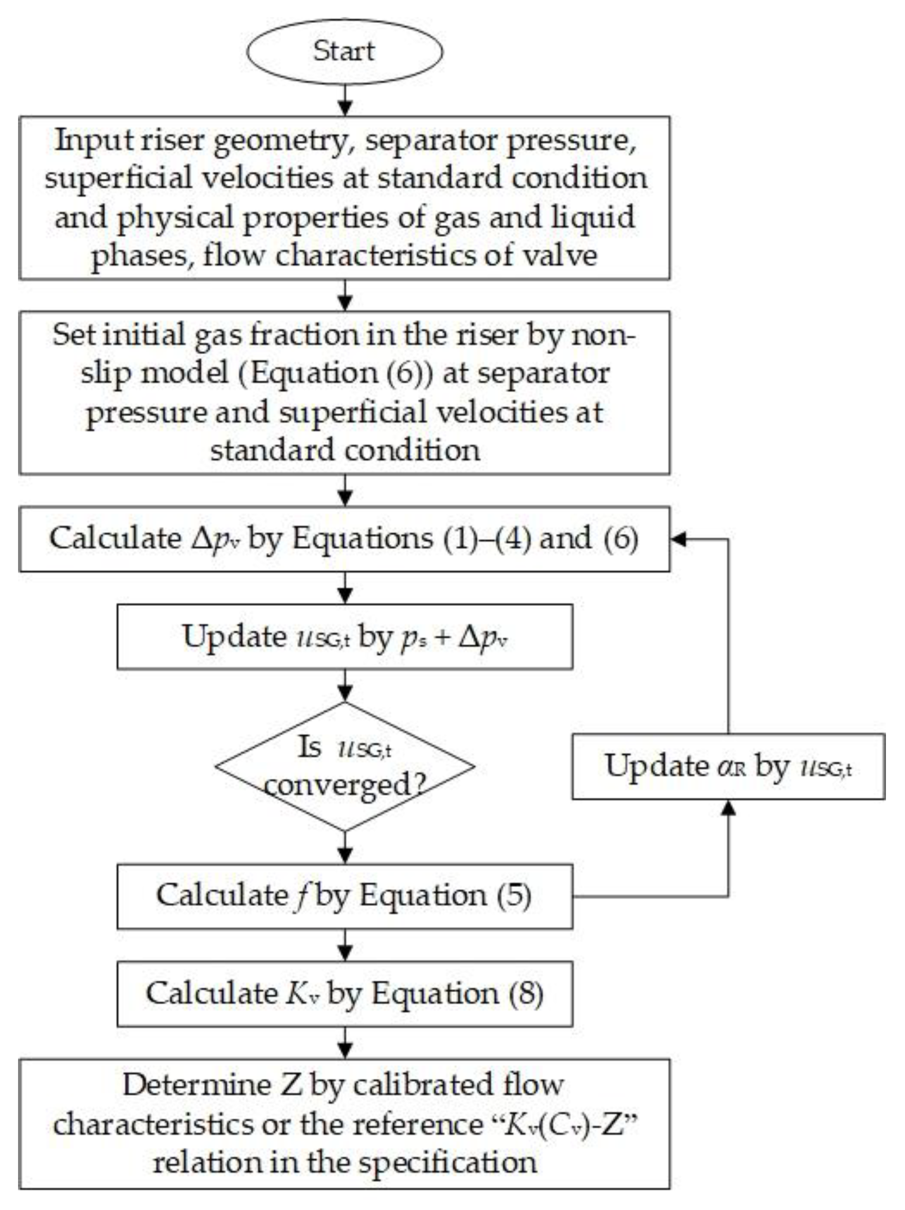
3. Derivation of Optimal Valve Opening
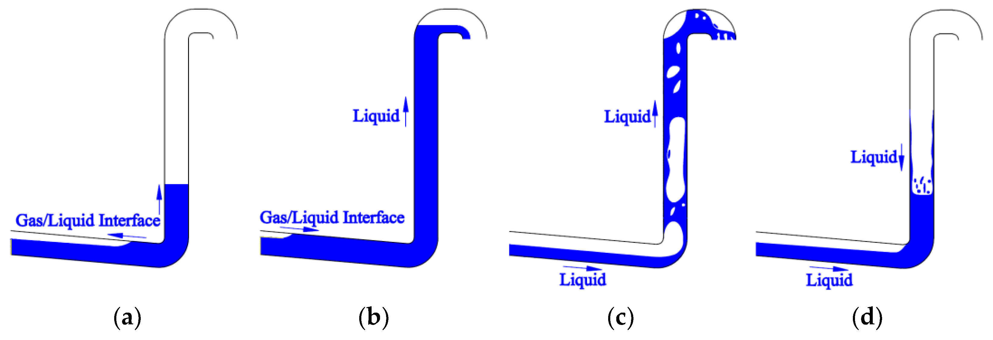
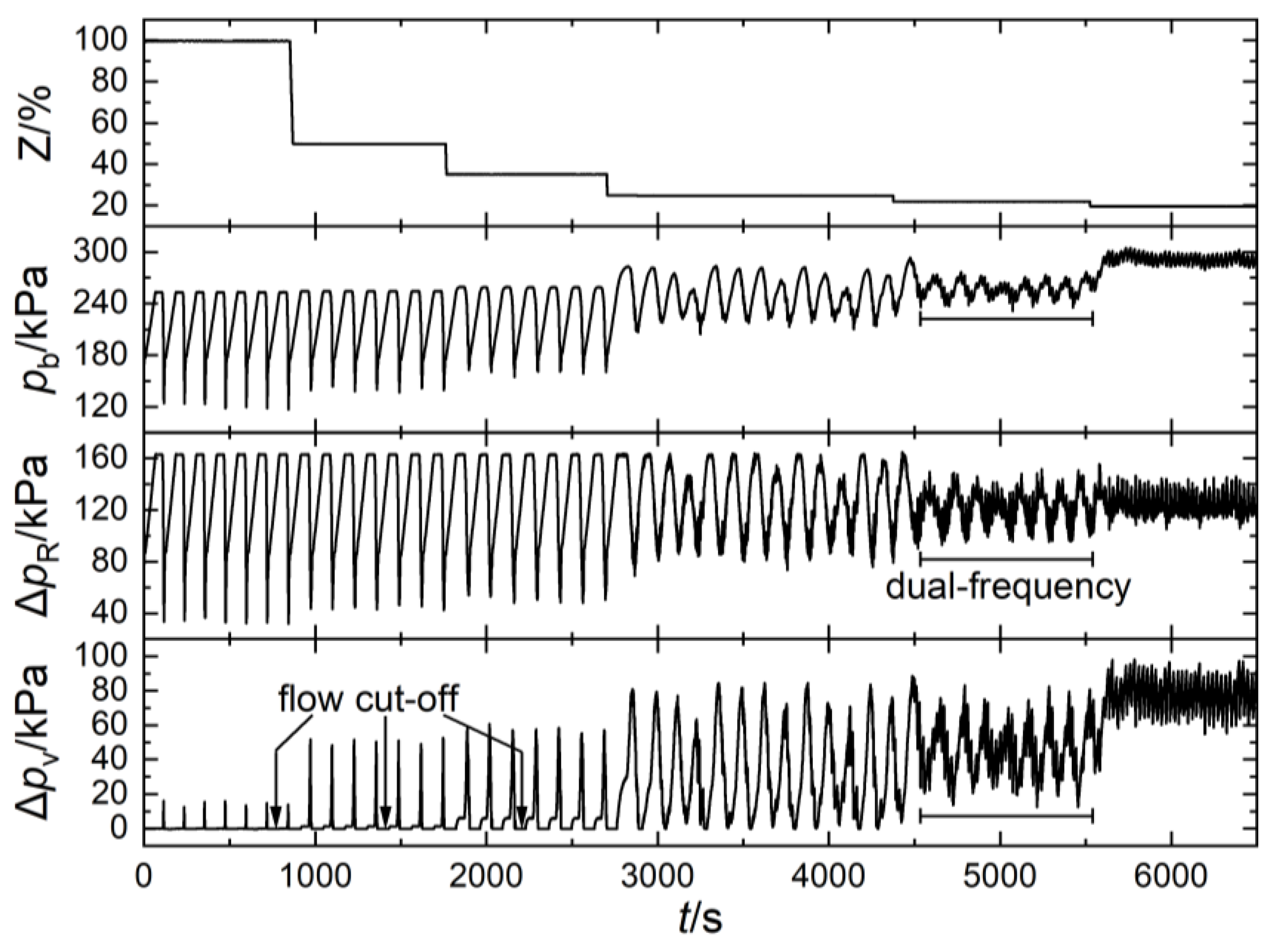
3.1. Target of Control
3.2. Macroscopic Flow Parameters at Optimal Condition
3.3. Optimal Valve Opening
4. Validation
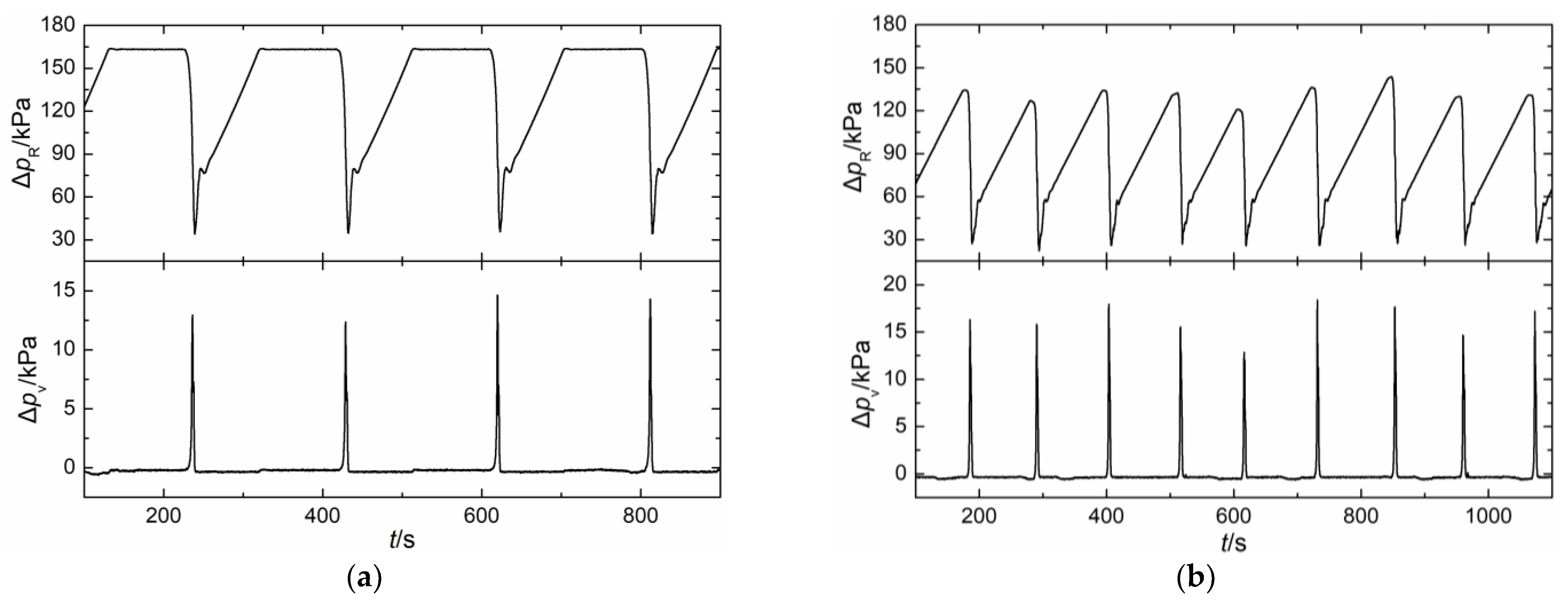
4.1. Laboratory Results and Discussion
4.2. Field Case
4.3. Discussion on Application
5. Conclusions
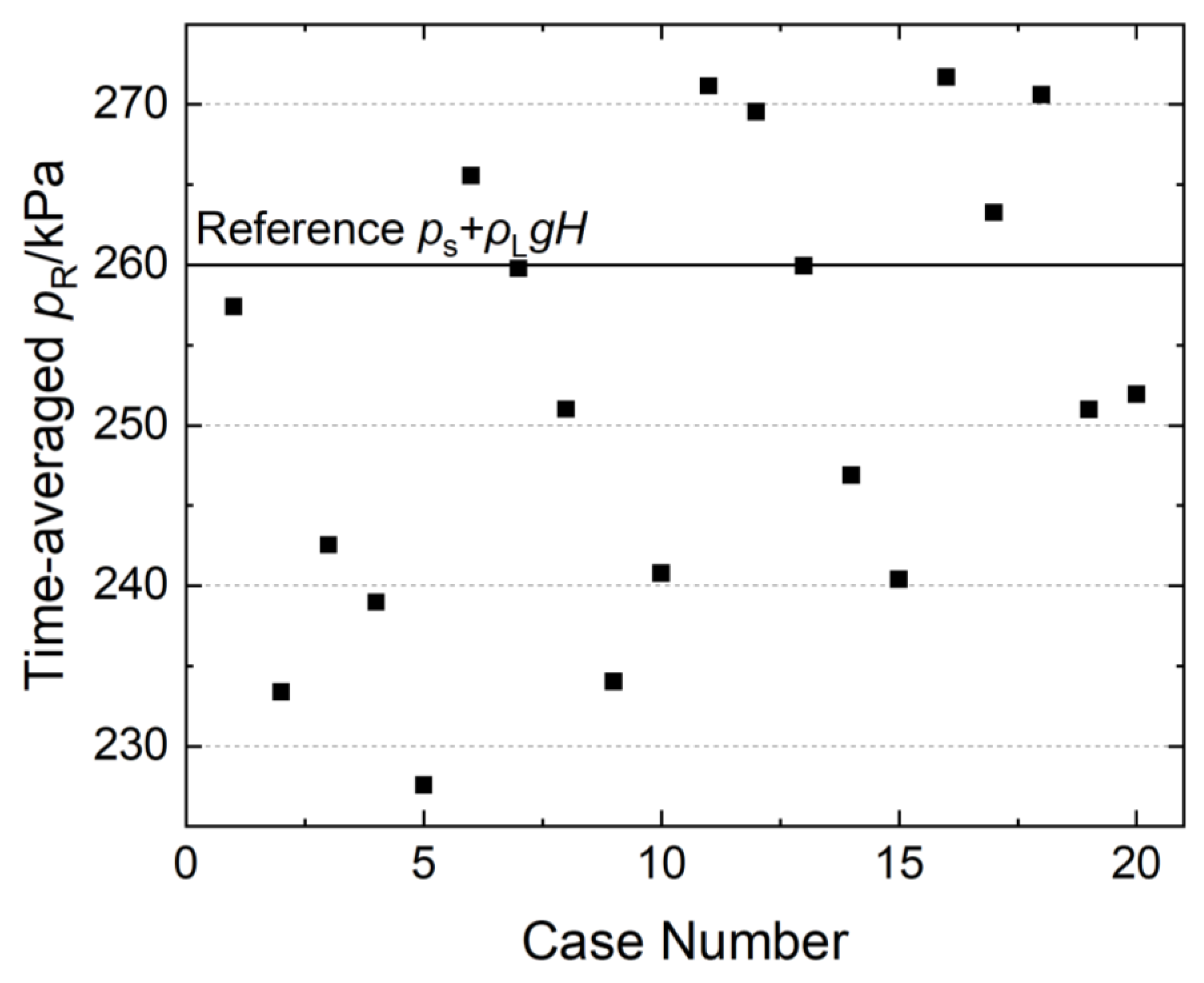
- The target of slugging control can be set as the occurrence of dual-frequency fluctuation. At the time, the sum of the time-averaged total pressure drop along the riser and that across the valve is approximately the same as the gravity pressure drop of single-phase water in the riser without choking. So, the conservation of total pressure drop can be assumed.
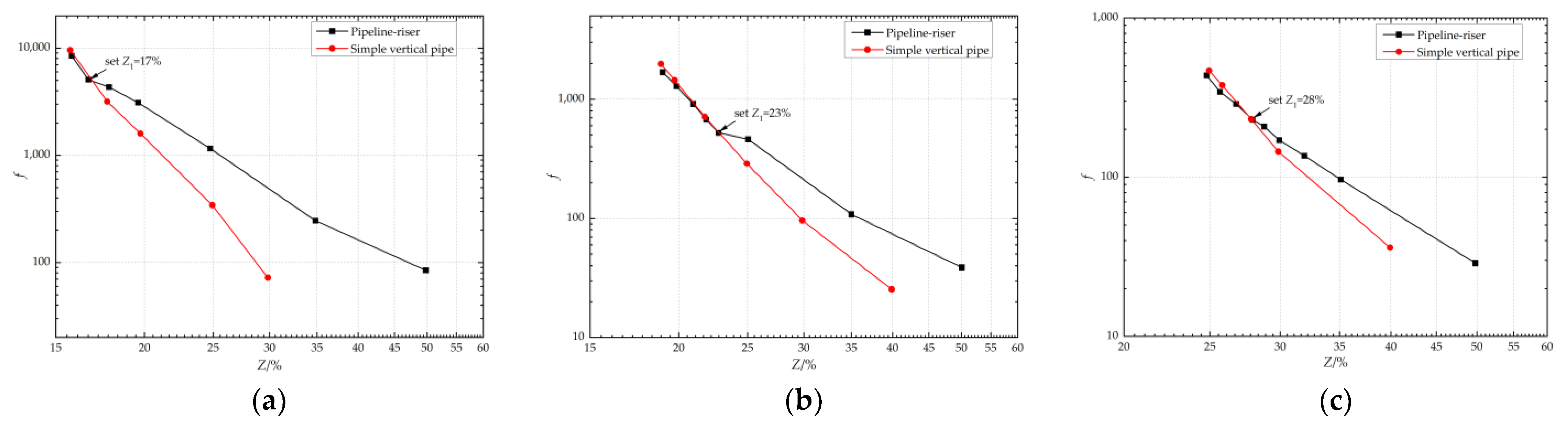
- The resistance factor of the valve is approximately the same as slug flow in a simple vertical pipe at the time severe slugging is eliminated, indicating the feasibility of calculating the resistance factor by a two-phase flow model in a simple vertical pipe.
- Because of severe flow intermittency in pipeline risers and weaker gas drift flow, and in order to be consistent with the processing of measured data, the non-slip assumption is recommended in the calculation of the gas fraction in the riser.
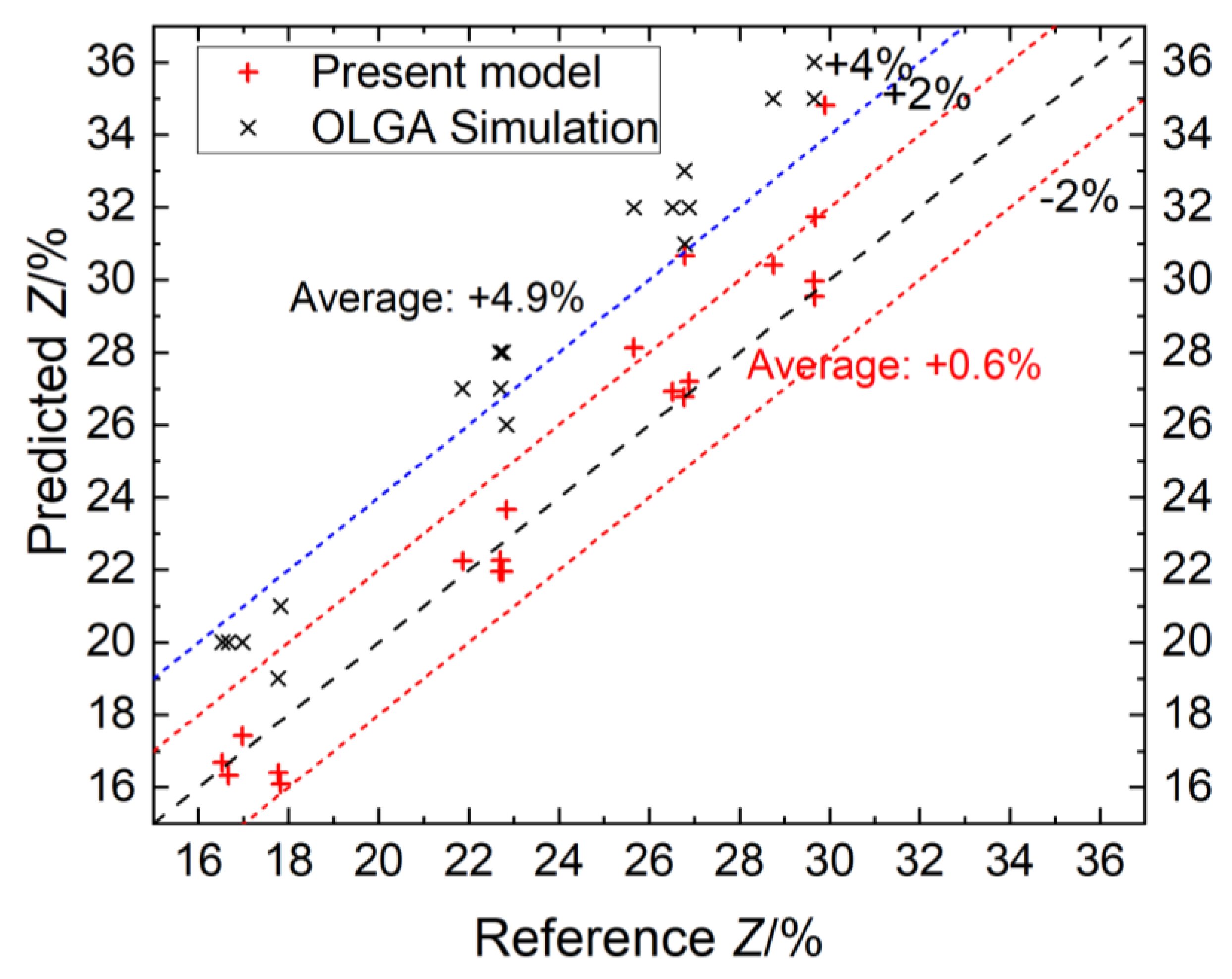
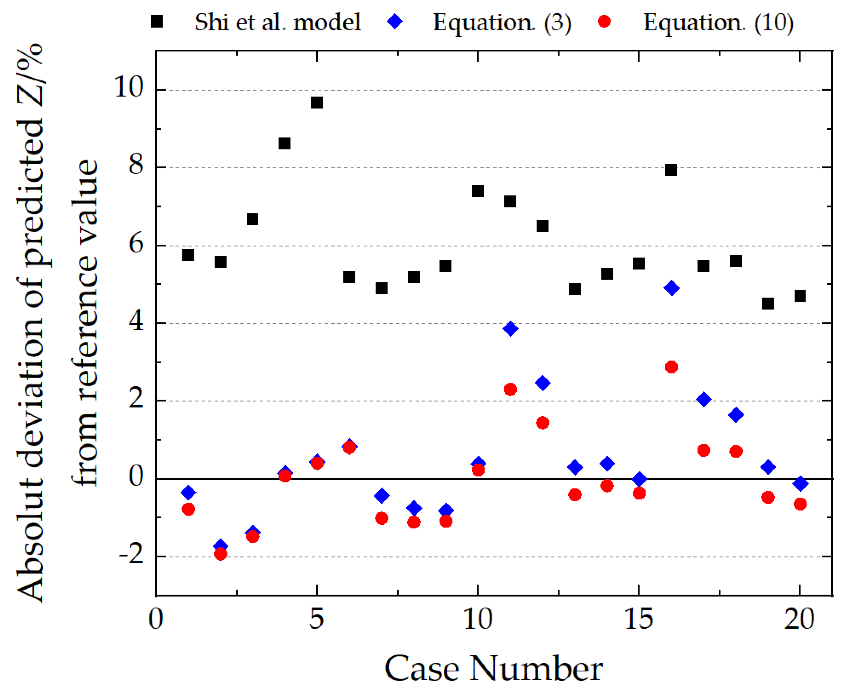
- The average absolute error of the proposed model is +0.01%, which is smaller than the simulation performed by OLGA software (+4.91% before tuning and +0.08% after tuning). The validation of the field case also proves the good applicability of the model (with deviation smaller than ±2%).
- Future work can focus on the application of the model to the valve selection at the design stage and the modification of the model for different valve installation positions on a real platform at the operation stage.
Author Contributions
Funding
Data Availability Statement
Acknowledgments
Conflicts of Interest
Abbreviations
| A | Area, m2. |
| Cv | Flow coefficient, gal·min−1·psi−1 (usually omitted). |
| d | Diameter, m. |
| f | Resistance factor, dimensionless. |
| g | Gravitational acceleration, 9.80665 m·s−2. |
| H | Height of riser, m. |
| Kv | Flow coefficient, m3·h−1·(105Pa)−1 (usually omitted). |
| p | Pressure, Pa. |
| Δp | Differential pressure, Pa. |
| Q | Mass flow rate, m3/d. |
| T | Temperature, K. |
| u | Velocity, m/s. |
| Z | Valve opening, %. |
| Greek letters | |
| ρ | Density, kg/m3. |
| α | Gas fraction, dimensionless. |
| σ | Surface tension, N·m. |
| Subscripts | |
| avg | Average. |
| b | Riser bottom. |
| G | Gas. |
| L | Liquid. |
| mix | Gas–liquid mixture. |
| R | Riser. |
| S | Superficial. |
| s | Separator. |
| t | Riser top. |
| 0 | Standard condition: at 101,325 Pa and 273.15 K for laboratorial experiments and at 100,000 Pa and 288.75 K for the field case. |
References
- Li, X.; Yue, Y.; Du, H.; Yue, L.; Ding, R.; Liu, C.; Li, Y. Investigation on leakage detection and localization in gas-liquid stratified flow pipelines based on acoustic method. J. Pipeline Sci. Eng. 2022, 3, 100127. [Google Scholar] [CrossRef]
- Sun, W.; Zhang, J.; Mukhtar, Y.; Zuo, L.; Dong, S. Safety Evaluation Method for Submarine Pipelines Based on a Radial Basis Neural Network. Sustainability 2023, 15, 12724. [Google Scholar] [CrossRef]
- Qiao, W.; Guo, H.; Huang, E.; Chen, H.; Lian, C. Two-Phase Flow Pattern Identification by Embedding Double Attention Mechanisms into a Convolutional Neural Network. J. Mar. Sci. Eng. 2023, 11, 793. [Google Scholar] [CrossRef]
- Yu, H.; Xu, Q.; Cao, Y.; Huang, B.; Guo, L. Effects of riser height and pipeline length on the transition boundary and frequency of severe slugging in offshore pipelines. Ocean. Eng. 2024, 298, 117253. [Google Scholar] [CrossRef]
- Banjara, V.; Pereyra, E.; Avila, C.; Murugavel, D.; Sarica, C. Improved severe slugging modeling and mapping. Geoenergy Sci. Eng. 2025, 244, 213446. [Google Scholar] [CrossRef]
- Schmidt, Z. Experimental Study of Two-Phase Slug Flow in a Pipeline-Riser Pipe System. Ph.D. Dissertation, University of Tulsa, Tulsa, OK, USA, 1977. [Google Scholar]
- Tengesdal, J.Ø. Investigation of Self-Lifting Concept for Severe Slugging Elimination in Deep-Water Pipeline/Riser Systems. Ph.D. Thesis, University of Tulsa, Tulsa, OK, USA, 2002. [Google Scholar]
- Malekzadeh, R.; Henkes, R.A.W.M.; Mudde. Severe slugging in along pipeline–riser system: Experiments and predictions. Int. J. Multiph. Flow 2012, 46, 9–21. [Google Scholar] [CrossRef]
- Henriot, V.; Courbot, A.; Heintzé, E.; Moyeux, L. Simulation of Process to Control Severe Slugging: Application to the Dunbar Pipeline. In Proceedings of the 1999 SPE Annual Technical Conference and Exhibition, Houston, TX, USA, 3–6 October 1999. [Google Scholar] [CrossRef]
- Havre, K.; Stornes, K.O.; Stray, H. Taming slug flow in pipelines. ABB Rev. 2000, 46, 55–63. [Google Scholar]
- Li, Z.; Luo, J.; Lu, J. Application and Analysis about Affection and Treatment of Slug Flow in BZ25-1 Oil Field. Shipbuild. China 2012, 53, 310–315. (In Chinese) [Google Scholar]
- Li, C.; Wu, W.; Zhang, L. Numerical simulation on control measures of severe slug flow in Boxi Oilfield. Oil Gas Storage Transp. 2018, 37, 95–100. (In Chinese) [Google Scholar] [CrossRef]
- Zhang, X.; Li, N.; Chen, B. Analysis and treatment on the severe slug flow in pipeline S-shaped riser of Wenchang Oilfield. Oil Gas Storage Transp. 2019, 38, 472–480. (In Chinese) [Google Scholar] [CrossRef]
- Bai, Y.; Bai, Q. Subsea Pipelines and Risers, 1st ed.; Elsevier Ltd.: Oxford, UK, 2005; pp. 277–316. [Google Scholar] [CrossRef]
- Pedersen, S.; Bram, M.V. The Impact of Riser-Induced Slugs on the Downstream Deoiling Efficiency. J. Mar. Sci. Eng. 2021, 9, 391. [Google Scholar] [CrossRef]
- Li, X.; Liu, Y.; Abbassi, R.; Khan, F.; Zhang, R. A Copula-Bayesian approach for risk assessment of decommissioning operation of aging subsea pipelines. Process Saf. Environ. 2022, 167, 412–422. [Google Scholar] [CrossRef]
- Liu, Y.; Zhu, X.; Song, J.; Wu, H.; Zhang, S.; Zhang, S. Research on bypass pigging in offshore riser system to mitigate severe slugging. Ocean. Eng. 2022, 246, 110606. [Google Scholar] [CrossRef]
- Zheng, G.; Xu, P.; Li, L.; Fan, X. Investigations of the Formation Mechanism and Pressure Pulsation Characteristics of Pipeline Gas-Liquid Slug Flows. J. Mar. Sci. Eng. 2024, 12, 590. [Google Scholar] [CrossRef]
- Banjara, V.; Pereyra, E.; Avila, C.; Sarica, C. Critical review & comparison of severe slugging mitigation techniques. Geoenergy Sci. Eng. 2023, 228, 212082. [Google Scholar] [CrossRef]
- Nnabuife, S.G.; Tandoh, H.; Whidbore, J.F. Slug flow control using topside measurements: A review. Chem. Eng. J. Adv. 2022, 9, 100204. [Google Scholar] [CrossRef]
- Ogazi, A.I. Multiphase Severe Slugging Flow Control. Ph.D. Thesis, Cranfield University, Cranfield, UK, 2011. [Google Scholar]
- Park, K.-H.; Kim, T.-W.; Kim, Y.-J.; Lee, N.; Seo, Y. Experimental investigation of model-based IMC control of severe slugging. J. Petrol. Sci. Eng. 2021, 204, 108732. [Google Scholar] [CrossRef]
- Jahanshahi, E.; Skogestad, S. Simplified Dynamical Models for Control of Severe Slugging in Multiphase Risers. IFAC Proc. Vol. 2011, 44, 1634–1639. [Google Scholar] [CrossRef]
- Guo, L.; Li, N.; Ye, J.; Chen, S. Choking Device and Method for Real-Time Eliminating Severe Slugging in a Pipeline-Riser System. Patent CN102410391B, 10 July 2013. [Google Scholar]
- Pedersen, S.; Durdevic, P.; Yang, Z. Learning control for riser-slug elimination and production-rate optimization for an offshore oil and gas production process. IFAC Proc. 2014, 47, 8522–8527. [Google Scholar] [CrossRef]
- Jansen, F.E.; Shoham, O.; Taitel, Y. The elimination of severe slugging: Experiment and modeling. Int. J. Multiph. Flow. 1996, 22, 1055–1072. [Google Scholar] [CrossRef]
- Fadairo, A.; Obi, C.; Li, K.; Rasouli, V.; Aboaba, O.; Gbadamosi, O. An improved model for severe slugging stability criteria in offshore pipeline-riser systems. Petrol. Res. 2022, 7, 318–328. [Google Scholar] [CrossRef]
- Pedersen, S.; Durdevic, P.; Yang, Z. Challenges in slug modeling and control for offshore oil and gas productions: A review study. Int. J. Multiph Flow 2017, 88, 270–284. [Google Scholar] [CrossRef]
- Andreolli, I.; Azevedo, G.R.; Baliño, J.L. Application of stability solver for severe slugging considering a choking device and a tubing connected to a Wet Christmas Tree. J. Petrol. Sci. Eng. 2020, 192, 107316. [Google Scholar] [CrossRef]
- Gong, J.; Kang, Q.; Wu, H.; Li, X.; Shi, B.; Song, S. Application and prospects of multi-phase pipeline simulation technology in empowering the intelligent oil and gas fields. J. Pipeline Sci. Eng. 2023, 3, 100127. [Google Scholar] [CrossRef]
- Zou, S.; Yao, T.; Guo, L.; Li, W.; Wu, Q.; Zhou, H.; Xie, C.; Liu, W.; Kuang, S. Non-Uniformity of Gas/Liquid Flow in a Riser and Impacts of Pipe Configuration and Operation on Slugging Characteristics. Exp. Therm. Fluid Sci. 2018, 96, 329–346. [Google Scholar] [CrossRef]
- Wang, H.; Zou, S.; Liu, T.; Xu, L.; Du, Y.; Yan, Y.; Guo, L. Experimental investigation of online solving for critical valve opening for eliminating severe slugging in pipeline-riser systems. Int. J. Heat Fluid Flow 2024, 110, 109584. [Google Scholar] [CrossRef]
- Al-Safran, E.M.; Kelkar, M. Predictions of Two-Phase Critical-Flow Boundary and Mass-Flow Rate Across Chokes. SPE Prod. Oper. 2009, 24, 249–256. [Google Scholar] [CrossRef]
- Shi, H.; Holmes, J.A.; Durlofsky, L.J.; Aziz, K.; Diaz, L.R.; Alkaya, B.; Oddie, G. Drift-Flux Modeling of Two-Phase Flow in Wellbores. SPE J. 2005, 10, 24–33. [Google Scholar] [CrossRef]
- Ye, J.; Guo, L. Multiphase flow pattern recognition in pipeline–riser system by statistical feature clustering of pressure fluctuations. Chem. Eng. Sci. 2013, 102, 486–501. [Google Scholar] [CrossRef]
- Ye, J.; Guo, L.; Xie, C.; Xu, Q. Experiment Study on Phase Inversion of Oil-water Two Phase Flow Using Double-parallel-ring Conductance Probe. J. Eng. Thermophys. 2010, 31, 983–986. (In Chinese) [Google Scholar]
- IEC 60534-2-4:2009; Industrial-Process Control Valves. Part 2-4: Flow Capacity-Inherent Flow Characteristics and Rangeability. International Electrotechnical Commission: Geneva, Switzerland, 2009.
- Zhao, X. Study on Transition Mechanism and Control Method of Severe Slugging in High-pressure Pipeline-riser System. Ph.D. Dissertation, Xi’an Jiaotong University, Xi’an, China, 2024. (In Chinese). [Google Scholar]


| Transmitter | Manufacturer | Transmitter Model | Range | Accuracy |
|---|---|---|---|---|
| Orifice Flowmeter (L) | YOKOGAWA | EJA-115 | 0–1.35 m3·h−1 | ±1% F.S. |
| Orifice Flowmeter (M) | YOKOGAWA | EJA-115 | 0–0.22 m3·h−1 | ±1% F.S. |
| Orifice Flowmeter (S) | YOKOGAWA | EJA-115 | 0–0.027 m3·h−1 | ±1% F.S. |
| Electromagnetic Flowmeter (L) | YOKOGAWA | AE204MG | 0–42.5 m3·h−1 | ±0.5% F.S. |
| Electromagnetic Flowmeter (S) | YOKOGAWA | AE115MG | 0–6.36 m3·h−1 | ±0.5% F.S. |
| Mass Flowmeter (L) | Siemens | Mass 6000 | 0–80 kg·h−1 | ±0.1% F.S. |
| Mass Flowmeter (S) | Emerson | CMF 010 | 0–24 kg·h−1 | ±0.1% F.S. |
| Pressure (P5/pb) | Micro | MPM480 | 0–500 kPa | ±0.25% F.S. |
| Differential Pressure (DP5/ΔpR) | Rosemount | 3051CD3 | −20–200 kPa | ±0.15% F.S. |
| Differential Pressure (DP11/Δpv) | Rosemount | 3051CD3 | 0–240 kPa | ±0.15% F.S. |
| Differential Pressure (DP12) | Rosemount | 3051CD3 | 0–240 kPa | ±0.15% F.S. |
| No. | uSL (m/s) | uSG0 (m/s) | Peak Value of uSL at Outlet (m/s) | Ratio (Peak Over Average) |
|---|---|---|---|---|
| 1 | 0.10 | 0.10 | 0.176 | 1.76 |
| 2 | 0.10 | 0.25 | 0.188 | 1.88 |
| 3 | 0.10 | 0.60 | 0.154 | 1.54 |
| 4 | 0.10 | 1.00 | 0.171 | 1.71 |
| 5 | 0.25 | 0.10 | 0.355 | 1.42 |
| 6 | 0.25 | 0.25 | 0.398 | 1.59 |
| 7 | 0.25 | 0.60 | 0.387 | 1.55 |
| 8 | 0.25 | 1.00 | 0.447 | 1.79 |
| 9 | 0.45 | 0.10 | 0.564 | 1.25 |
| 10 | 0.45 | 0.25 | 0.591 | 1.31 |
| 11 | 0.45 | 0.60 | 0.713 | 1.58 |
| 12 | 0.45 | 1.00 | 0.601 | 1.34 |
| 13 | 0.60 | 0.10 | 0.775 | 1.29 |
| 14 | 0.60 | 0.25 | 0.750 | 1.25 |
| 15 | 0.60 | 0.60 | 0.772 | 1.29 |
| 16 | 0.60 | 1.00 | 0.719 | 1.20 |
| No. | uSL (m/s) | uSG0 (m/s) | Set Z1 * % | Set Z2 * % | f Ratio * at min (Z1, Z2) |
|---|---|---|---|---|---|
| 1 | 0.10 | 0.10 | 17 | 17 | 0.90 |
| 2 | 0.10 | 0.25 | 18 | 18 | 1.03 |
| 3 | 0.10 | 0.60 | 18 | 17 | 0.90 |
| 4 | 0.25 | 0.10 | 22 | 22 | 0.98 |
| 5 | 0.25 | 0.25 | 22 | 23 | 0.92 |
| 6 | 0.25 | 0.60 | 23 | 23 | 0.99 |
| 7 | 0.45 | 0.10 | 28 | 27 | 1.06 |
| 8 | 0.45 | 0.25 | 28 | 26 | 0.95 |
| 9 | 0.45 | 0.60 | 26 | 27 | 0.86 |
| 10 | 0.25 | 0.60 | 23 | 23 | 0.99 |
| Parameter | Value | Unit |
|---|---|---|
| H | 138.9 | m |
| dR | 250.9 | mm |
| ps,avg | 560 | kPa(a) |
| Twellhead | 329.25 | K |
| Tambient | 303.15 | K |
| QL | 1985 | m3/d |
| QG0 | 102,705 | m3/d |
| ρL | 850.7 | kg/m3 |
| ρG0 | 1.179 | kg/m3 |
| Δpv,avg | 566 | kPa |
| σ | 0.0691 | N·m |
| dv | 250 | mm |
| Cv,max | 1000 | gal·min−1·psi−1 |
| valve flow characteristic | equal percentage | - |
| Parameter | Value | Unit |
|---|---|---|
| αt (αv) | 0.7965 | |
| αb | 0.7673 | |
| αR | 0.7819 | |
| Δpv | 887.87 | kPa |
| uSL,v | 0.465 | m/s |
| uSG,v | 1.819 | m/s |
| ρmix,v | 185.52 | kg/m3 |
| f | 1810 | |
| Kv | 63.69 | m3·h−1·(105 Pa)−1 |
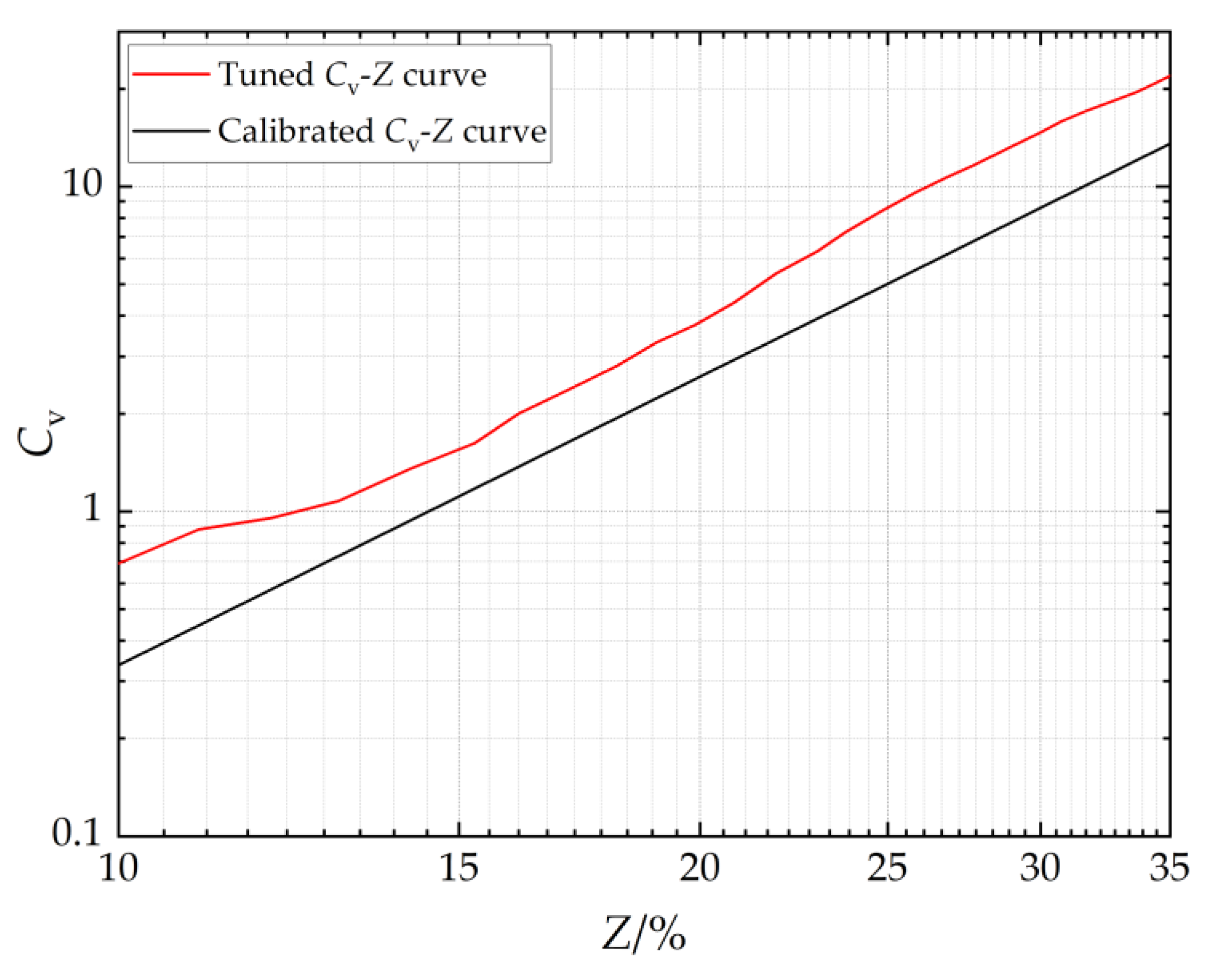
| Z | 33.06% (Equation (9)) |
| Rangeability | Definition of Rangeability | Predicted Z/% |
|---|---|---|
| 50 | Kv(Z = 100%)/Kv(Z = 0%) | 33.06% |
| 40 | Kv(Z = 100%)/Kv(Z = 0%) | 29.01% |
| 30 | Kv(Z = 100%)/Kv(Z = 0%) | 23.00% |
| 50 | Kv(Z = 100%)/Kv(Z = 5%) | 36.40% |
| 40 | Kv(Z = 100%)/Kv(Z = 5%) | 32.55% |
| 30 | Kv(Z = 100%)/Kv(Z = 5%) | 26.85% |
Disclaimer/Publisher’s Note: The statements, opinions and data contained in all publications are solely those of the individual author(s) and contributor(s) and not of MDPI and/or the editor(s). MDPI and/or the editor(s) disclaim responsibility for any injury to people or property resulting from any ideas, methods, instructions or products referred to in the content. |
© 2025 by the authors. Licensee MDPI, Basel, Switzerland. This article is an open access article distributed under the terms and conditions of the Creative Commons Attribution (CC BY) license (https://creativecommons.org/licenses/by/4.0/).
Share and Cite
Fu, J.; Wu, Q.; Sun, J.; Wang, H.; Zou, S. The Prediction of the Valve Opening Required for Slugging Control in Offshore Pipeline Risers Based on Empirical Closures and Valve Characteristics. J. Mar. Sci. Eng. 2025, 13, 981. https://doi.org/10.3390/jmse13050981
Fu J, Wu Q, Sun J, Wang H, Zou S. The Prediction of the Valve Opening Required for Slugging Control in Offshore Pipeline Risers Based on Empirical Closures and Valve Characteristics. Journal of Marine Science and Engineering. 2025; 13(5):981. https://doi.org/10.3390/jmse13050981
Chicago/Turabian StyleFu, Jiqiang, Quanhong Wu, Jie Sun, Hanxuan Wang, and Suifeng Zou. 2025. "The Prediction of the Valve Opening Required for Slugging Control in Offshore Pipeline Risers Based on Empirical Closures and Valve Characteristics" Journal of Marine Science and Engineering 13, no. 5: 981. https://doi.org/10.3390/jmse13050981
APA StyleFu, J., Wu, Q., Sun, J., Wang, H., & Zou, S. (2025). The Prediction of the Valve Opening Required for Slugging Control in Offshore Pipeline Risers Based on Empirical Closures and Valve Characteristics. Journal of Marine Science and Engineering, 13(5), 981. https://doi.org/10.3390/jmse13050981