The Effect of In-Pipe Fluid States and Types on Axial Stiffness Characteristics of Fiber-Reinforced Flexible Pipes

Abstract

As critical components in marine engineering fluid transmission systems, fiber-reinforced flexible (FRF) pipes have static mechanical properties that depend on internal fluid pressure. Current analytical approaches predominantly employ uniformly distributed load (UDL) assumptions to simulate unidirectional fluid pressure effects on pipe surfaces. However, existing methodologies neglect fluid–pipe structure coupling effects. This study investigates the rubber-based FRF pipe by establishing a numerical model incorporating fluid–structure interaction effects and material nonlinearity, aiming to explore how different fluid states (closed or constant pressure) and fluid types (incompressible or compressible) influence the mechanical behavior of the FRF pipe under axial loading. Experimental validation of the numerical model demonstrates that UDL assumptions remain valid for gas-filled pipes (both in the closed and constant pressure states) and the liquid-filled pipe in the constant pressure state. The incompressibility of the filled liquid significantly enhances pipe axial stiffness, invalidating the UDL approximation method in liquid-filled closed states. Furthermore, the asymptotic saturation model proposed effectively quantifies the liquid-induced enhancement in axial stiffness. The developed numerical model and derived conclusions provide valuable insights into structural design optimization, experimental protocol development, and practical engineering applications for FRF pipes.

1. Introduction

Fiber-reinforced flexible (FRF) pipes exhibit exceptional design versatility, where key parameters such as matrix material formulations, fiber reinforcement compositions, and ply stacking sequences can be optimized to meet performance requirements in diverse application scenarios [1,2]. This characteristic grants them broad application prospects in marine engineering [3,4,5,6]. Compared with conventional metal pipes, FRF pipes leverage their low stiffness and high compliance to achieve larger displacement adaptability and complex load-bearing capacity [7,8]. Moreover, they can serve as elastic damping elements to effectively mitigate vibration and impact induced pipeline damage [9,10]. Consequently, the mechanical performance of FRF pipes not only governs pipe system efficiency but also critically determines the safety and reliability of marine structures. Given that internal fluid pressure constitutes a dominant operational load during fluid transportation, investigation of its influence on the mechanical behavior of FRF pipes, such as axial stiffness and deformation, has significant engineering implications.

The mechanical performance and failure behavior of FRF pipes under static internal pressure loading have remained a focal research area. In theoretical investigations, Kruijer et al. [11] applied laminate theory to reinforced thermoplastic pipes, developing a nonlinear extended plane stress model that accounted for fiber reorientation and diameter variation during pressurization, thereby revealing the mechanical response of long pipes under hydrostatic pressure. Xia et al. [12] derived exact elastic solutions for stresses and deformations in multilayered filament-wound pipes under internal pressure using three-dimensional anisotropic elasticity theory. Subsequent work by Xing et al. [13] introduced axisymmetric thick-walled cylinder theory to analyze the mechanical behavior of multi-angle hybrid fiber-reinforced thick-walled cylinders under combined loads (internal/external pressure and axial force). Additionally, Gao et al. [14] investigated deformation responses of closed-end FRF pipes with helical stiffeners under internal pressure by employing Donnell approximations and Euler–Bernoulli beam theory. While these studies represent significant methodological advancements over simplified fiber-only models (e.g., Rogers et al. [15] and Evans et al. [16]), they relied on idealized material constitutive assumptions. Nevertheless, experimental validation by Gu et al. [17] demonstrated that approximating the polymeric matrix as a linear elastic material leads to substantial discrepancies between theoretical predictions and experimental results.

Fang et al. [5] addressed material nonlinearity in their investigation of glass fiber-reinforced flexible pipes under tension and internal pressure by iteratively updating material properties at each load increment. Building on this method, Wang et al. [18] introduced stress–strain curve fitting techniques to parameterize experimental material data, enabling material property updates. However, such methods are limited to scenarios where material nonlinearity is characterized under unidirectional loading conditions. Given the pronounced nonlinear behavior exhibited by polymeric matrices in FRF pipes under multiaxial stress states, hyperelastic constitutive models rooted in strain energy density functions provide an accurate representation of their complex mechanical responses [19]. The capability of numerical simulations to address material nonlinearity has established them as a pivotal tool for investigating FRF pipe mechanics under internal pressure. Representative studies include Tonnato et al. [20], who predicted burst pressures of floating composite pipes; and Pan et al. [4], who quantified the influence of fiber and rubber properties on pressure-deformation responses and failure pressures in helically ribbed composite marine pipes. These investigations collectively demonstrated the accuracy and reliability of numerical methodologies through experimental validation.

The above and other theoretical and numerical studies generally employ constant uniformly distributed load (UDL) to characterize the unidirectional mechanical effect between internal fluids and FRF pipes. To simulate end effects induced by internal pressure, conventional methods typically apply constant UDL or axial tension to pipe end plates. This idealized assumption overlooks fluid pressure redistribution resulting from pipe deformation and varying structural responses caused by different fluid states and types.

The fluid cavity method has emerged as an innovative solution to overcome these limitations and has been successfully implemented across multiple disciplines. Tong et al. [21] modeled blood as an incompressible fluid within cardiac and aortic cavities to investigate trauma mechanisms of aortic rupture during occupant–vehicle interior collisions; Ye et al. [22] simulated gas behavior in marine inflatable membrane structures, elucidating bending and failure characteristics under operational conditions; and Xiao et al. [23] analyzed stiffness–gas mass relationships in dual-wedge safety airbags for medical devices through gas containment simulations. Complementary studies [24,25] further extended this methodology to airbag systems and pneumatic tensegrity domes, respectively. These implementations collectively confirm the method’s versatility in simulating fluid–structure coupling phenomena, positioning it as an available tool for modeling various fluid states and types within FRF pipes.

This paper investigates rubber-based FRF pipes, focusing on their static mechanical response characteristics under axial loads. It specifically examines how differences in fluid states (closed state vs. constant pressure state) and fluid types (compressible type vs. incompressible type) influence the mechanical behavior of the pipes. Section 2 details the numerical modeling methodology for FRF pipes, including the fitting of the hyperelastic constitutive model for rubber materials, the construction of fluid–structure coupling models using the fluid cavity method, and the specification of meshing strategies and boundary conditions. Section 3 outlines the experimental design for testing the axial stiffness of FRF pipes. Section 4 presents a comparison and validation of numerical results against experimental results, analyzing the differential effects of fluid states and types on axial stiffness while exploring the applicability of UDL simulations and the sensitivity of fluid parameters. Finally, Section 5 summarizes the main conclusions, provides recommendations for engineering applications, and suggests directions for future research. It is important to note that the term “closed state” refers to the condition where the fluid is fully sealed within the pipe after pressurization, with no mass exchange occurring between the pipe and its external environment. Conversely, the “constant pressure state” denotes the condition where the fluid inside the pipe maintains a constant pressure during axial loading after pressurization. Additionally, “UDL simulations” refer to the simplification of the fluid force acting on the pipe wall as a uniformly distributed load perpendicular to the inner surface of the pipe.

This study is the first to apply the fluid cavity method to FRF pipe research, constructing a numerical model that incorporates material nonlinearity and fluid–structure coupling effects, thereby overcoming the limitations of the traditional UDL assumption. Through numerical simulations and experimental validation, it is demonstrated that the strong coupling effect induced by the incompressibility of liquid under the closed state renders the UDL assumption invalid. Furthermore, the study quantitatively separates the contributions of structural stiffness and liquid stiffness, elucidating the nonlinear enhancement mechanism of axial stiffness by the liquid bulk modulus. This provides a new reference for static fluid–structure coupling research in FRF pipes.

2. Numerical Modeling of the Fiber-Reinforced Flexible Pipe

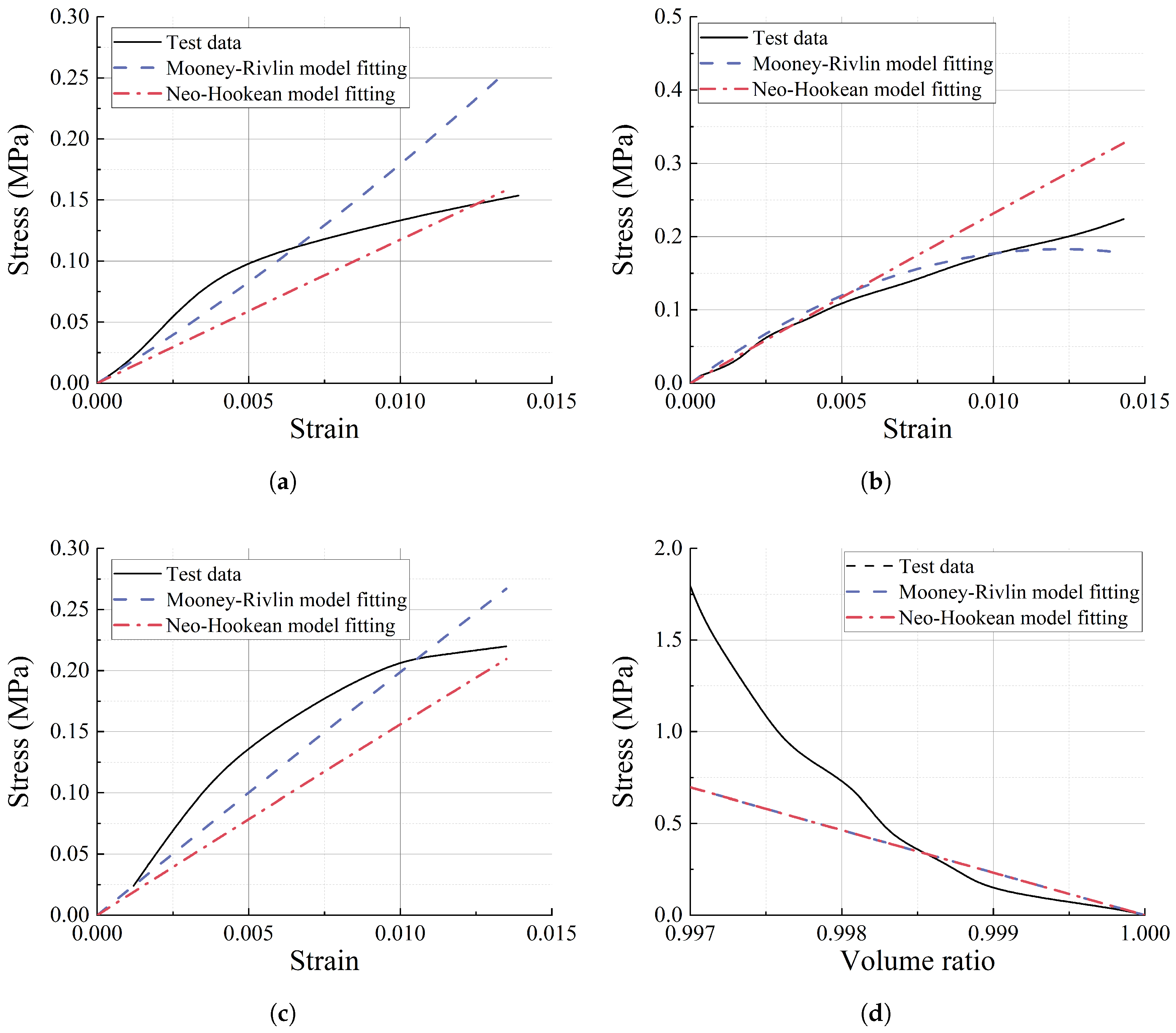
2.1. Material Characterization and Hyperelastic Constitutive Modeling

Rubber materials exhibit multiaxial stress coupling characteristics under complex deformation modes. To accurately characterize their mechanical behavior, this study conducts uniaxial tension, equibiaxial tension, planar tension, and volumetric compression tests. And stress–strain data of the material are obtained to determine the material parameters required for input into the numerical model. The experimental setup and rubber specimens are illustrated in Figure 1. All specimens are sectioned from 2 mm thick rubber sheets that share identical curing histories with the matrix material of the FRF pipe.

All experiments are conducted under controlled ambient temperature (23 ± 2 °C). Uniaxial tension, planar tension, and volumetric compression tests are performed using a WDW-10 testing machine, which is manufactured by E-RUBBER Technology (Beijing, China), with a maximum capacity of 10 kN. Biaxial tension testing employs a specialized system consisting of fixtures, a clamp drive system, and a multi-axis sensor array. After specimen installation, initial clamp adjustments ensure zero-stress states by eliminating residual tension or bending moments. Quasi-static loading is applied at strain rates of 0.01 mm/s (0.02 mm/s for volumetric compression). Deformation measurements are obtained using laser extensometry tracking displacement between two central white fiducial markers, as shown in Figure 1. To mitigate Mullins effects [27,28], the testing strain rates are kept similar to those experienced by FRF pipes produced by the Naval University of Engineering (Wuhan, China).

To characterize the hyperelastic behavior of rubber materials, a parameterized constitutive relationship is established using experimentally obtained stress–strain data. The strain energy function U is formulated based on three strain invariants $I_1$, $I_2$, and $I_3$, which collectively provide a complete deformation characterization [29]:

$$U=f\left(I_1,I_2,I_3\right),$$

(1)

Due to the incompressibility of rubber, the third strain invariant is constrained as $I_3\equiv 1$. The remaining invariants are kinematically related to the principal stretch ratios (${\lambda }_1$, ${\lambda }_2$, ${\lambda }_3$) via the following constitutive definitions:

$$\left\{\begin{array}{c}{I}_1={\lambda }_1^2+{\lambda }_2^2+{\lambda }_3^2\\ I_2={\lambda }_1^2{\lambda }_2^2+{\lambda }_2^2{\lambda }_3^2+{\lambda }_3^2{\lambda }_1^2\end{array}\right.,$$

(2)

The Mooney–Rivlin and Neo-Hookean constitutive models are widely employed in the literature to describe strain energy functions [30]. Their mathematical representations are defined as follows:

$$\begin{array}{c}U=C_{10}\left(I_1-3\right)+C_{01}\left(I_2-3\right)+{\displaystyle \frac{1}{D_1}}{\left(J_{el}-1\right)}^2\hfill \\ U=C_{10}\left(I_1-3\right)+{\displaystyle \frac{1}{D_1}}{\left(J_{el}-1\right)}^2\hfill \end{array},$$

(3)

The Mooney–Rivlin model incorporates the second strain invariant $I_2$, serving as an extended formulation of the Neo-Hookean model. The material constants $C_{10}$ and $C_{01}$ govern shear behavior, while $D_1$ denotes the compressibility coefficient and $J_{el}$ represents the elastic volume ratio. The material testing results and model fitting for the rubber are presented in Figure 2, where the fitting process is conducted using Abaqus software. The experimental data indicate that the material does not exhibit a stiffening effect with increasing strain (as evidenced by the absence of upward curvature in the stress–strain curve). Consequently, there is no need to employ models incorporating higher-order strain invariants for fitting (e.g., the Ogden model or Yeoh model). Although the Mooney–Rivlin model introduces the second strain invariant $I_2$ to enhance adaptability under multi-axial stress conditions, the negative value obtained in the fitting result ($C_{01}=-50.3$) leads to instability in the material’s constitutive behavior. This instability is specifically manifested by the anomalous points shown in Figure 2b, where stress decreases with increasing strain. In contrast, all parameters of the Neo-Hookean model ($D_1=8.62\times {10}^{-3}$, $C_{10}=1.98$) are positive. This can be attributed to the relatively minor conformational changes in the rubber molecular chains under small-strain conditions, where entropic elasticity deformation likely dominates as the primary deformation mechanism. Given its ability to provide a simple yet accurate approximation [29], the Neo-Hookean model is selected for the final fitting results.

2.2. Development of the Numerical Model

The FRF pipe is manufactured through a vulcanization process integrating a rubber matrix with fiber reinforcement layers. Featuring a triple-flange configuration at both ends, the pipe comprises four reinforcement layers with complementary winding angles embedded within the rubber matrix (innermost layer winding angle is $53.1^{\circ }$ relative to the axial direction). Detailed reinforcement fiber parameters are summarized in

Table 1. Reinforced fiber material parameters.

Parameter	Value
Density (t/mm3)	$1.44\times {10}^{-9}$
Young’s modulus (MPa)	$3.28\times {10}^4$
Poisson’s ratio	0.36

.

To facilitate installation and ensure post-installation sealing integrity, the flanges are designed with structural features including bolt holes, bosses, and chamfers. For computational efficiency, these detailed features are omitted from the geometry model. Furthermore, geometric simplifications are applied at the intermediate flange region, where the rubber matrix and reinforcement fibers are mechanically constrained, as illustrated in Figure 3.

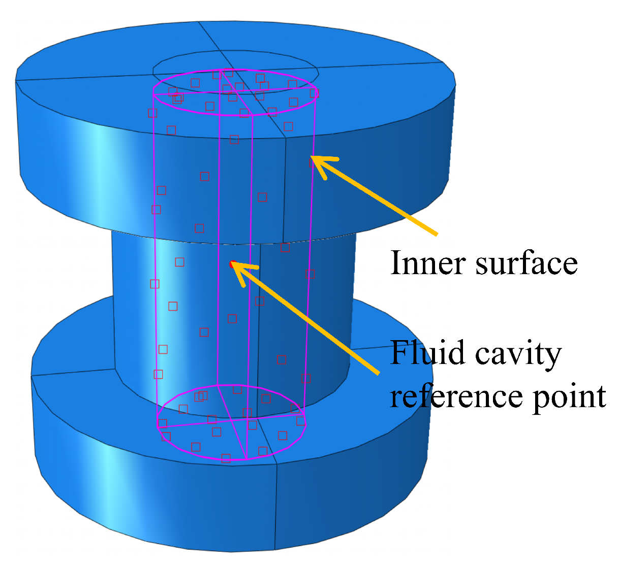
2.2.1. Fluid–Structure Coupling Model Based on the Fluid Cavity Method

When modeling liquid-filled FRF pipes, the liquid bulk modulus $K_{liquid}$ is introduced to account for fluid incompressibility. Assuming that $K_{liquid}$ remains independent of liquid density, the internal pressure $p_{liquid}$ can be expressed as:

$$\begin{array}{c}{p}_{liquid}=-K\left({\rho }_{liquid}^{-1}\left(p,\theta \right)-{\rho }_{liquid0}^{-1}\left(\theta \right)\right)\hfill \end{array},$$

(4)

where ${\rho }_{liquid}$ and ${\rho }_{liquid0}$ denote the final and initial liquid densities, respectively, p represents the final pressure, and $\theta$ indicates temperature. Assuming ideal gas behavior for the internal gas, the pipe pressure $p_{gas}$ can be expressed using the ideal gas equation of state as:

$$\begin{array}{c}{p}_{gas}={\rho }_{gas}R\left(\theta -{\theta }^Z\right)\hfill \end{array},$$

(5)

where ${\rho }_{gas}$ denotes gas density, ${\theta }^Z$ represents absolute temperature, and R is the gas constant defined as the ratio of the universal gas constant to the molecular weight of the ideal gas. It should be explicitly noted that temperature effects are excluded in this investigation, and in constant pressure states, the internal fluid pressure remains invariant. Additionally, the fluid cavity model is implemented by selecting all inner surfaces of the FRF pipe and defining a cavity reference node (see Figure 4). This reference node has a single degree of freedom governing pressure variation within the cavity. To simulate diverse fluid behaviors, nitrogen and water are selected as representative compressible and incompressible media, with their material parameters summarized in

Table 2. Parameters of the fluid cavity model.

Parameter		Value
Water	Density (t$/{\mathrm{mm}}^3$)	$1\times {10}^{-9}$
	Bulk modulus (MPa)	2100
Nitrogen	The molecular weight of the ideal gas (t/mol)	$2.8\times {10}^{-5}$

.

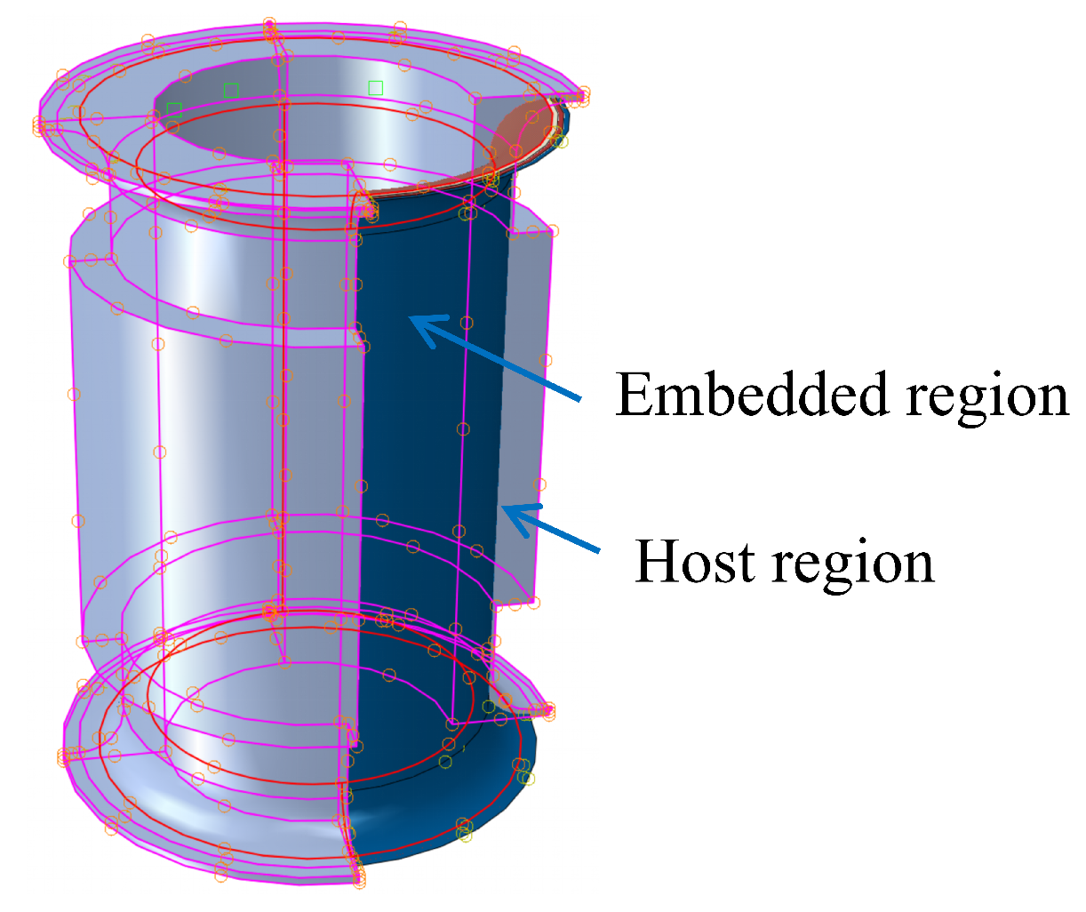
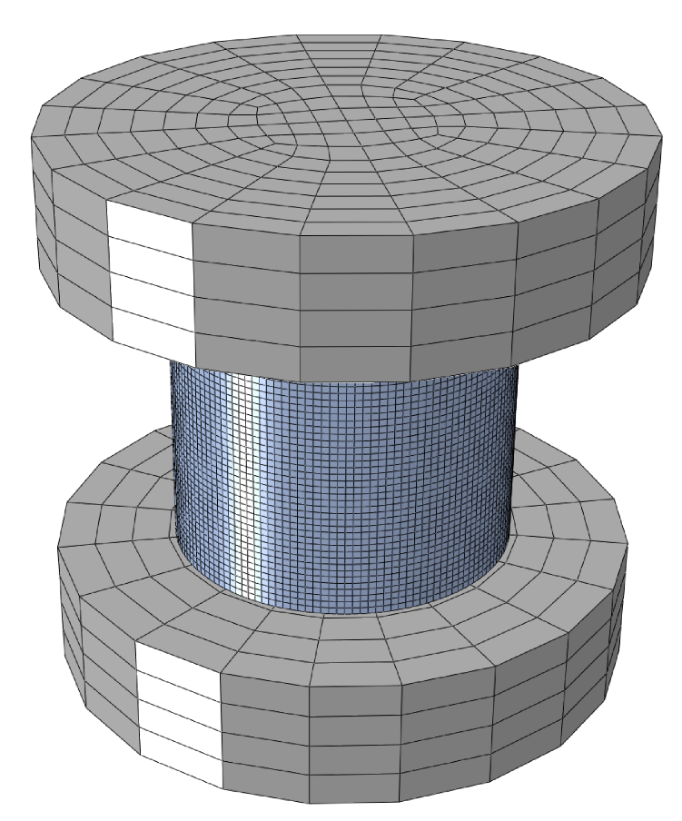
2.2.2. Interaction, Meshing, and Boundary Conditions

The vulcanization process induces dense chemical crosslinking networks at the rubber–fiber interface, thereby enabling efficient stress transfer between matrix and reinforcement. Consequently, the rubber–fiber interfacial interactions are simulated using an embedded region constraint (as illustrated in Figure 5). Within this modeling approach, the nodal displacements of the reinforcement fiber elements are computed by interpolating displacements from adjacent to the rubber matrix elements.

The developed FRF pipe numerical model is illustrated in Figure 6, where the rubber matrix and fiber reinforcement layers are discretized using C3D8R and M3D4R elements, respectively, and the total mesh comprises 131,616 elements. The flange components, manufactured from cast copper alloy and carbon structural steel, exhibit mechanical strength properties that significantly exceed those of the rubber matrix and reinforcement fibers. As a result, these flanges are modeled as rigid bodies and excluded from the computational domain to improve computational efficiency.

Since the material of the flange is cast copper alloy and carbon structural steel, whose strength far exceeds that of the rubber matrix and the reinforcing fiber material, the flange is simplified as a rigid body in the model and does not participate in the calculation. In establishing the numerical model, the rubber matrix and the fiber-reinforced layer are modeled using C3D8R and M3D4R elements, respectively. To ensure the grid independence of the numerical model and determine the computational cost, the axial stiffness of the FRF pipe is calculated for four different grid sizes when the pipe is filled with water and in the closed state (

Table 3. Grid convergence analysis (water-filled closed state, initial pressure of 1 MPa).

Grid Size (mm)	Total Number of Elements	Axial Stiffness (N/mm)	Relative Error (vs. Grid Size 1.5 mm)	Calculation Time (s)
3	49,233	1389.65	−6.31%	91
2.5	83,081	1437.74	−3.07%	171
2	131,616	1465.04	−1.23%	284
1.5	306,649	1483.29	-	2466

). The results indicate that the error monotonically converges as the grid is refined. Specifically, the error for the grid with a unit size of 2 mm is only 1.23%. Regarding computational time, the grid with a unit size of 2 mm requires 284 s (AMD Ryzen 9 7940H, 16GB memory), which is only 11.52% of the time required for the grid with a unit size of 1.5 mm. Therefore, considering both accuracy and efficiency, a numerical model established with a grid size of 2 mm is adopted for subsequent analysis (as shown in Figure 6).

In the numerical model, the motion of both end flanges is kinematically constrained to their respective reference points. To simulate the pressure charging and axial loading processes, two analysis steps are implemented. As shown in Figure 7a, during the first analysis step, both flanges are fixed while fluid pressure is applied by controlling the degree of freedom at the fluid cavity reference node, thereby simulating the pressurization process. In the second analysis step, the bottom flange remains fixed, and axial loading is applied via displacement control at the top flange (see Figure 7b). The fluid pressure control strategy involves two operational conditions:

• Closed state simulation: The fluid cavity pressure control is deactivated after the first analysis step, effectively trapping initially pressurized fluid within the pipe;
• Constant pressure state simulation: The fluid pressure applied in the first analysis step is maintained throughout the second analysis step, ensuring invariant internal pressure during axial loading.

Figure 7. Multi-step boundary conditions: (a) Pressurization process. (b) Axial displacement process.

Figure 7. Multi-step boundary conditions: (a) Pressurization process. (b) Axial displacement process.

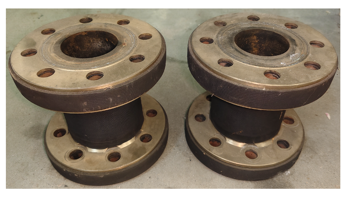
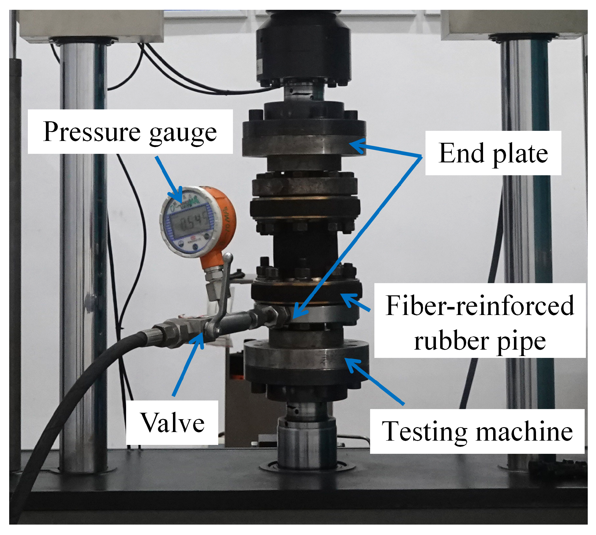
3. Axial Stiffness Testing of Fiber-Reinforced Flexible Pipes

The predictive accuracy of the numerical model is validated through axial stiffness testing of the FRF pipe. To ensure the reliability of experimental results, two FRF pipe specimens are prepared for axial stiffness testing (as shown in Figure 8). The specimens have nominal dimensions of 166 mm in length, 65 mm in inner diameter, and 100 mm in outer diameter. Measurement results indicate maximum deviations between actual and nominal dimensions of 0.2 mm (length) and 5.73 mm (outer diameter), corresponding to relative errors of 0.12% and 5.73%, respectively. These minor deviations suggest that the manufacturing process demonstrates satisfactory dimensional consistency.

The axial stiffness testing of FRF pipes is conducted using an MTS testing machine, with the experimental setup shown in Figure 9. The FRF pipe is connected to the testing apparatus through end plates, where the lower end plate features a through-port for interfacing with fluid transfer lines that connect the pipe to a pressurization pump and accumulator. The accumulator serves to maintain constant internal pressure. A pressure gauge integrated into the fluid transfer line allows for real-time pressure monitoring. The test configuration further includes a pressure-regulating valve for fluid pressure control. To achieve quasi-static loading conditions, a displacement rate of 0.1 mm/s is applied during axial loading within a ±2 mm range.

The FRF pipe has a maximum working pressure of 1.6 MPa. To prevent negative pressure development during axial loading, which could impair pressure gauge and valve performance, a target pressure of 1.5 MPa is selected. Prior to axial loading, the FRF pipe is pressurized to the target pressure, after which the valves are closed to simulate mechanical behavior in the closed state. With valves kept open, the accumulator ensures constant fluid pressure, enabling mechanical response characterization in the constant pressure state. Notably, nitrogen and water are employed as working fluids. However, due to the limitations of the accumulator equipment, constant-pressure testing is exclusively conducted with water as the internal medium.

4. Results and Discussion

4.1. Numerical Results and Experimental Validation of FRF Pipe Axial Stiffness

The axial stiffness values averaged from specimen 1 and specimen 2 are compared with numerical results in

Table 4. Error between experimental mean axial stiffness and numerical results.

State	Fluid	Axial Stiffness (N/mm)		Error
		Numerical	Experimental
Closed	Water	$1567.06$	$1583.09$	$-1.01$%
	Nitrogen	$1248.7$	$1245.12$	$0.29$%
Constant pressure	Water	1288.23	1271.47	$1.32$%

, revealing a maximum deviation of 1.32% between numerical and experimental results. The primary error source originates from the manual tensioning process during reinforcement layer fabrication. Workers typically split and stretch the sulfurized cord fabric ends at the intermediate flange (see Figure 10), inadvertently introducing unintended prestress into the structure. Furthermore, discrepancies exist between the fitted hyperelastic constitutive model and material test data (Figure 2). Given the small magnitude of maximum error, the numerical model demonstrates effective predictive capability for FRF pipe axial stiffness under various fluid states and types.

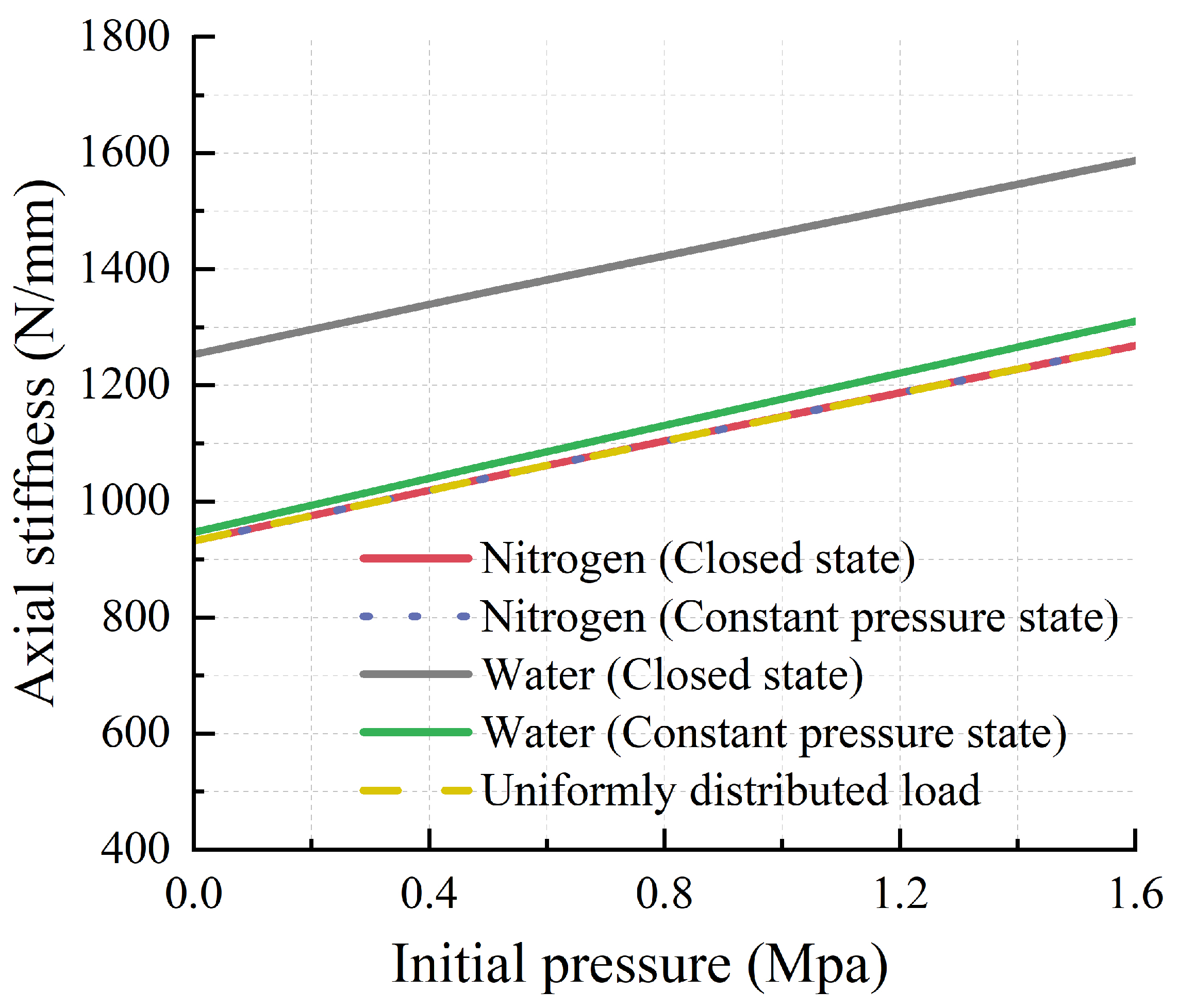
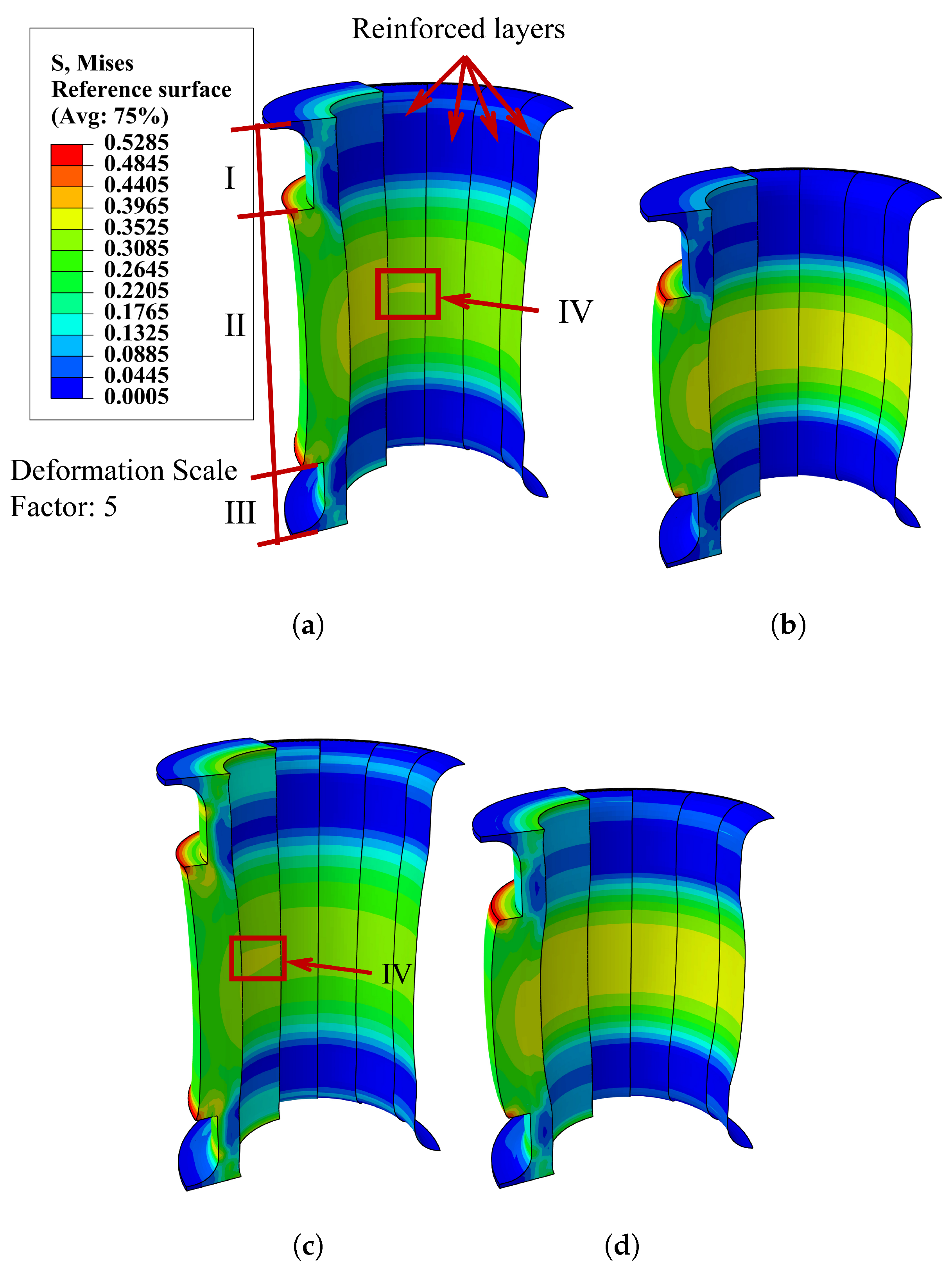
4.2. Effects of Fluid States and Types on Axial Stiffness

Using the established numerical model, the axial stiffness of the FRF pipe is calculated across an initial internal pressure range of 0 MPa to 1.6 MPa (the maximum working pressure of the test specimens), with additional simulations incorporating UDL application on the inner pipe surface. As shown in Figure 11, when the pipe contains nitrogen (in both closed state and constant pressure state), its axial stiffness aligns with the UDL-based simulation results. This indicates weak fluid–structure coupling between nitrogen and the FRF pipe, as nitrogen primarily exerts uniformly distributed normal pressure on the inner pipe surface. Therefore, regardless of the nitrogen containment state, its pressure effects can be simplified as UDL.

Furthermore, Figure 11 demonstrates that the axial stiffness of the nitrogen-filled FRF pipe increases progressively with rising internal pressure. To elucidate this pressure-dependent stiffening mechanism, stress distributions in both the rubber matrix and four-layer cord fabric reinforcement are comparatively analyzed at internal pressures of 0.5 MPa and 1 MPa. For consistency in comparison, all subplots in Figure 12 adopt identical stress contour legends.

As shown in Figure 12, significant stress differentials are observed between the inner and outer pipe surfaces, as well as along the central cross-section toward the axial ends. These spatially heterogeneous stress distributions collectively confirm the establishment of a three-dimensional stress state within the FRF pipe structure. Under identical tensile or compressive loading conditions with the same internal pressure, stress magnitudes progressively decrease with increasing pipe radius, indicating stress redistribution facilitated by the rubber matrix’s cushioning effect. Flange constraints effectively suppress deformation in regions I and III. Under tensile loading, region II exhibits concave inward deformation. The higher internal pressure in Figure 12c reduces stress magnitudes in this region compared to Figure 12a, demonstrating enhanced resistance to radial deformation due to increased pressure. Conversely, compressive loading induces outward convexity in region II, where internal pressure elevates stress levels in Figure 12d relative to Figure 12b, highlighting pressure-dependent stress amplification. Notably, irregular stress distributions emerge in regions IV, attributed to angular deviations between cord fabric orientation and pipe axis.

Figure 11 reveals that in the constant pressure water-filled state, the axial stiffness of FRF pipes marginally exceeds the UDL simulation result. Beyond stiffness variations, Figure 13 comparatively illustrates deformation characteristics of the inner pipe diameter under both loading conditions. During the pressurization and compression loading, the stiffness of the water in the pipe (the pressure required to maintain its state) is higher than under pure mechanical loading, leading to reduced deformation. In the axial tensile loading, the UDL can partially counteract the contraction, resulting in minimal deformation. Tension causes the pipe to contract, which increases the water pressure. Simultaneously, the reduction in pressure weakens the resistance to contraction, thereby causing more pronounced deformation. According to Figure 11, the maximum discrepancy between water pressurization and UDL-based axial stiffness reaches 3.32%. Furthermore, minor deformation discrepancies between both conditions (as shown in Figure 13) validate the mechanical equivalence of simplifying constant pressure water effects as UDL.

In contrast, when the FRF pipe is in a closed state and contains water, its axial stiffness is significantly higher than under other conditions. At zero internal pressure, the axial stiffness is 34.52% greater than that observed under nitrogen-filled conditions. To investigate the underlying mechanisms driving this fluid-type-dependent stiffness variation in closed systems, the variation patterns of fluid volume and pressure during axial loading are analyzed. As shown in Figure 14, the horizontal axis represents computational time, with the intervals 0–1, 1–1.5, and 1.5–2 corresponding to the pressurization, axial tension, and axial compression processes, respectively. Additionally, the legend annotation “initial pressure” refers to the internal pressure stabilized at the end of the 0–1 pressurization step.

Figure 14 illustrates distinct fluid-dependent behaviors under axial loading. Significant cavity volume changes occur under axial loads when the pipe contains nitrogen, while pressure variations remain relatively negligible due to the compressibility of nitrogen. In contrast, when the pipe contains water, smaller volume changes are observed. Specifically, under tensile loading, volume reduction induces a substantial pressure increase (e.g., from an initial pressure of 0.8 MPa to a final pressure of 1.85 MPa, exceeding the specimen’s maximum working pressure). Under compressive loading, volume expansion causes a pressure reduction (e.g., from initial pressure of 0.4 MPa to final pressure of −0.08 MPa, resulting in negative pressure). These findings highlight risks of excessive or negative pressure-induced failure in water-filled systems.

It can be assumed that the incompressibility of water inherently constrains pipe deformation, while the resulting deformation conversely induces pressure variations within the water medium. This synergistic interaction between the fluid’s incompressibility and structural deformation significantly enhances the axial stiffness of the FRF pipe. Consequently, theoretical analyses and numerical simulations must explicitly account for water’s coupling effects rather than the approximating water-filled closed state as UDL. Furthermore, when modeling end forces induced by internal pressure via equivalent axial forces, special attention must be paid to pressure-dependent force fluctuations during axial loading.

4.3. Effects of Fluid Parameters on the Axial Stiffness of the FRF Pipe in the Closed State

In the closed state, the axial stiffness of the FRF pipe is intrinsically linked to the physical properties of the filled fluid. As summarized in Table 2, the behavior of gases is characterized by their molecular weights, while the incompressibility of liquids is quantified through their bulk moduli. Based on molecular weight data of common gases from Reference [31], axial stiffness is calculated for gaseous media with molecular weights ranging from $1.5\times {10}^{-5}$ t/mol to $4.5\times {10}^{-5}$ t/mol, encompassing common gases such as oxygen, carbon dioxide, and carbon monoxide. For liquids, a bulk modulus range of 500–2500 MPa is selected, covering typical values for crude oil, liquefied natural gas, and methanol. The computational results are graphically presented in Figure 15.

As shown in Figure 15, the axial stiffness of the FRF pipe demonstrates no correlation with the molecular weight of ideal gases, indicating that the gas type has a negligible effect on the pipe structure. This observation further validates the conclusion that fluid–structure interactions are weak in gas-filled systems. Conversely, in liquid-filled systems, the axial stiffness increases with bulk modulus, albeit with diminishing enhancement rates. This is because liquids with a higher bulk modulus generate substantial counteracting forces against pipe deformation. However, as bulk modulus continues to increase, the liquid’s contribution to stiffness asymptotically saturates, resulting in reduced sensitivity of axial stiffness to further modulus increments.

For liquid-filled pipes, Figure 15 demonstrates that the axial stiffness $k_{total}$ of FRF pipes in the closed state is determined by both structural stiffness and fluid incompressibility. For gas-filled pipes, the incompressibility contribution is negligible, leading to $k_{gas}$ being governed solely by structural properties. Considering the asymptotic saturation of liquid-induced stiffness as the bulk modulus increases, an asymptotic saturation model is proposed:

$$\begin{array}{c}{k}_{total}=k_{\mathrm{gas}}+{\displaystyle \frac{\alpha K_{liquid}}{K_{liquid}+\beta }}\hfill \end{array},$$

(6)

where $\alpha$ denotes the saturation stiffness (the limiting value of liquid-induced stiffness), and $\beta$ represents the bulk modulus at half-saturation. Parameter identification is performed through nonlinear least-squares minimization of the sum of squared errors (SSE):

$$\begin{array}{c}SSE={\sum }_{i=1}^{17}{\left[k_{total,i}-\left(k_{gas}-{\displaystyle \frac{\alpha K_{liquid,i}}{\beta +K_{liquid,i}}}\right)\right]}^2\hfill \end{array},$$

(7)

Fitting yields $\alpha =367.59\pm 0.4$ N/mm and $\beta =327.3\pm 1.8$ MPa, as shown in Figure 15b. The model achieves a coefficient of determination $R^2=0.99$ with a root mean square error of 0.437 N/mm, demonstrating excellent predictive capability. Using the structural stiffness from Table 4 (nitrogen-filled closed state) and the bulk modulus of water from Table 2, the calculated axial stiffness of the FRF pipe filled with water in the closed state is 1563.14 N/mm, which differs by only −1.26% from the experimental result in Table 4.

5. Conclusions

This study establishes a numerical model that incorporates fluid–structure interactions between static internal fluids and the FRF pipe, with the aim of analyzing mechanical responses under axial loading across diverse fluid conditions. The maximum discrepancy between numerically predicted and experimentally measured axial stiffness is 1.3%, thereby validating the model’s reliability. Key findings are summarized as follows:

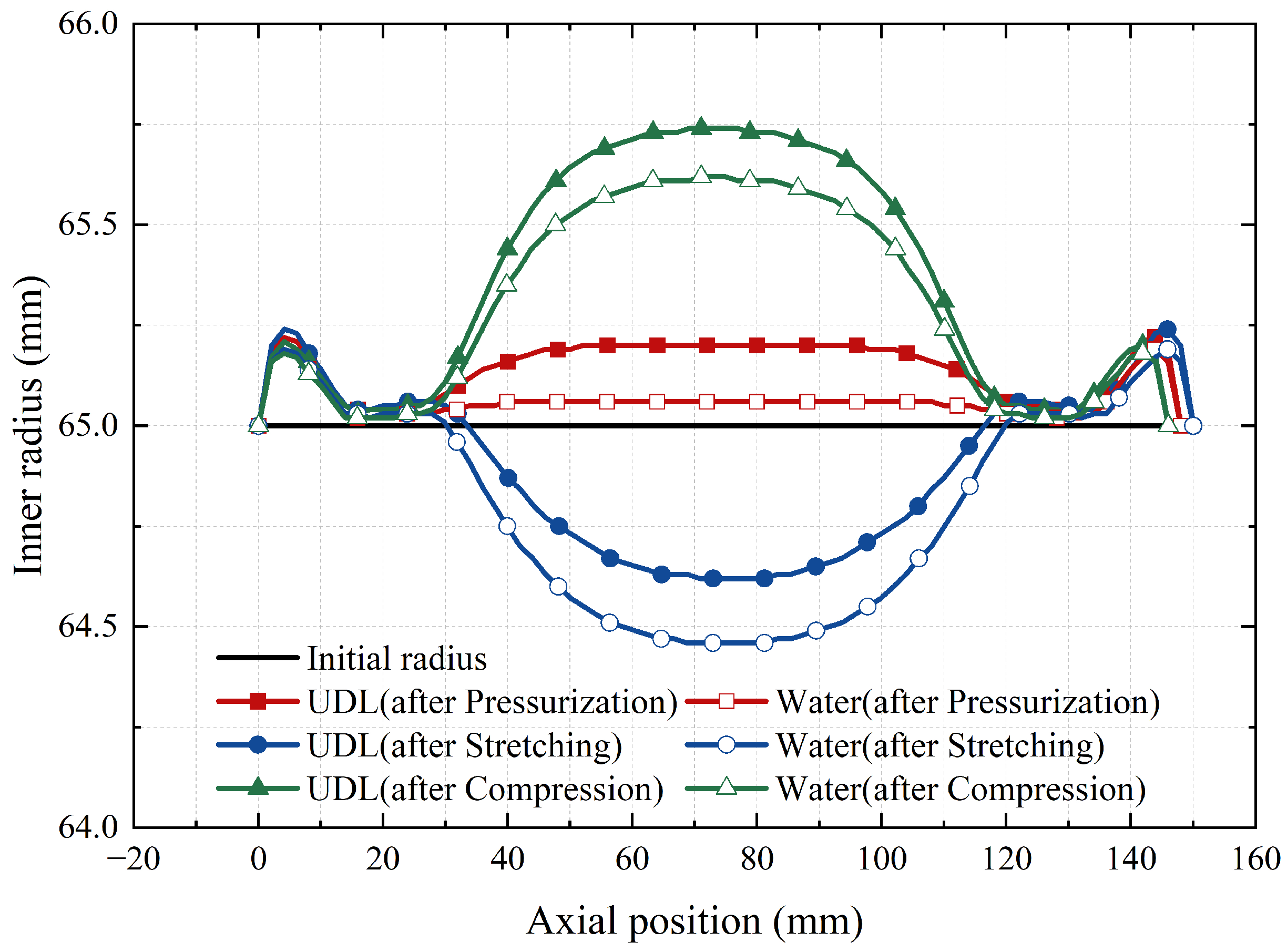
• Weak fluid–structure coupling allows gas-induced loads to be simplified as UDL in both the closed and constant pressure states. This simplification remains valid for the water-filled constant pressure state as well;
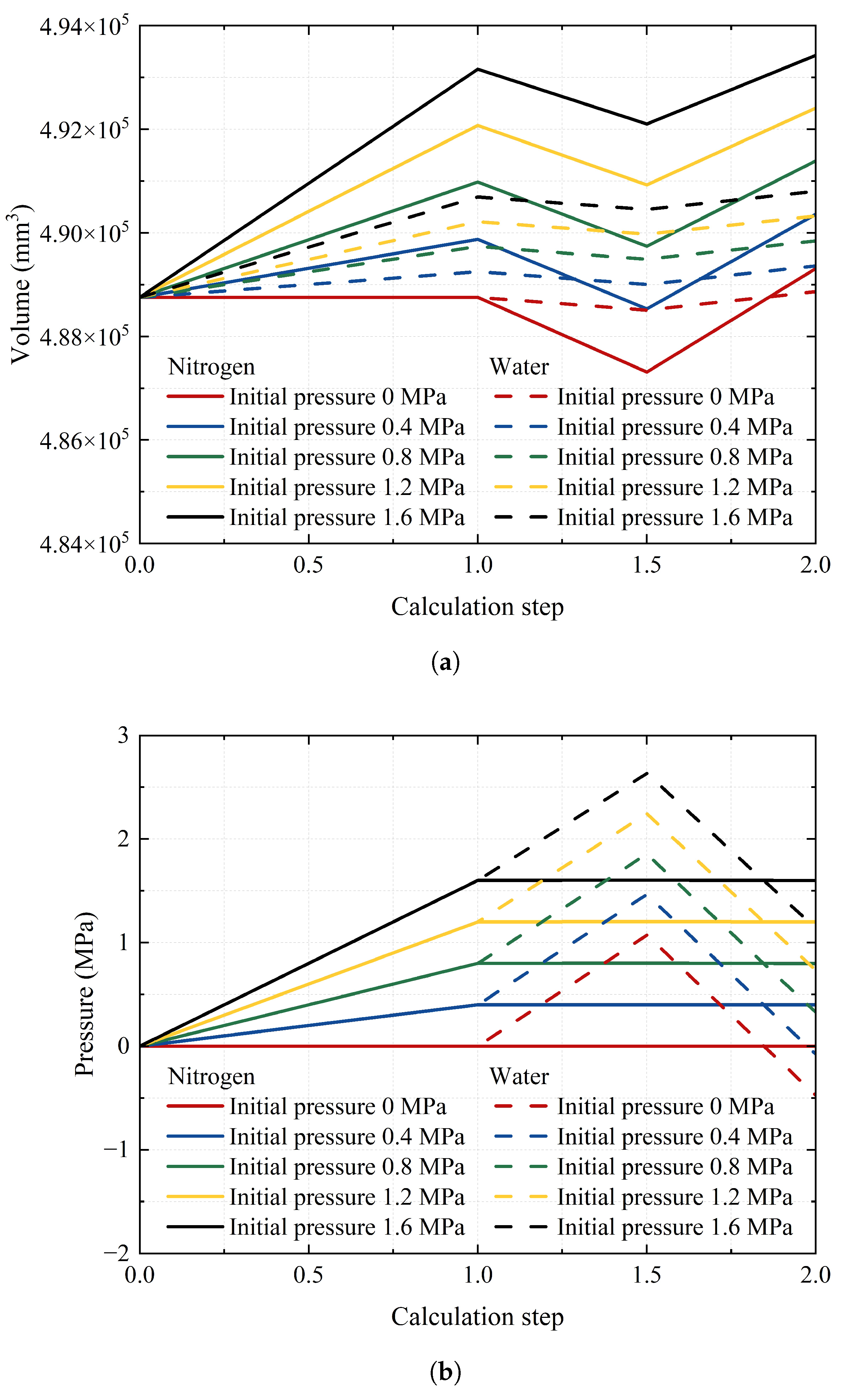
• In the closed state, when water serves as the internal fluid of the pipe, the strong coupling effect between water’s incompressibility and the pipe structure precludes the simplification of the force exerted by water on the pipe as UDL. Additionally, during axial loading, significant fluctuations in water pressure may result in the internal pipe pressure exceeding or falling below the allowable pressure range specified for the pipe design. Furthermore, particular attention should be given to the fact that end effects induced by water pressure no longer manifest as a constant force;
• In the closed state, there is a positive correlation between the bulk modulus of the liquid and the axial stiffness of the FRF pipe. By establishing an asymptotic saturation model, the quantitative relationship between the structural stiffness of the pipe and the stiffness contribution from the liquid is elucidated. This formula decouples structural stiffness from liquid effects, ensuring that it degrades to the gas-condition result at low bulk modulus values and asymptotically approaches the upper limit of the combined structural–fluid stiffness at high bulk modulus values.

In summary, this work elucidates the critical influence of fluid states and types on the axial stiffness of the FRF pipe, which can guide the design and optimization of FRF pipes in various engineering applications. Future research will further transcend the limitations of static fluid coupling analysis by focusing on the following directions to enhance engineering applicability: First, under actual complex operating conditions, explore the regulatory mechanisms of fluid viscosity and flow velocity on the axial stiffness of pipes. And under the matched asymptotic expansion, the research on the hydroelastic response can be extended by drawing on the work of Mohapatra et al. [32]. Second, incorporate a multiphysics coupling to comprehensively analyze the influence of factors such as temperature effects on the axial stiffness of FRF pipes, providing a theoretical foundation for their application in complex scenarios, including deep-sea energy transportation and ship power systems.

References

1. Alabtah, F.G.; Mahdi, E.; Eliyan, F.F. The use of fiber reinforced polymeric composites in pipelines: A review. Compos. Struct. 2021, 276, 114595. [Google Scholar] [CrossRef]
2. Diniță, A.; Ripeanu, R.G.; Ilincă, C.N.; Cursaru, D.; Matei, D.; Naim, R.I.; Tănase, M.; Portoacă, A.I. Advancements in Fiber-Reinforced Polymer Composites: A Comprehensive Analysis. Polymers 2023, 16, 2. [Google Scholar] [CrossRef] [PubMed]
3. Wei, D.; An, C.; Wu, C.; Duan, M.; Estefen, S.F. Torsional structural behavior of composite rubber hose for offshore applications. Appl. Ocean. Res. 2022, 128, 103333. [Google Scholar] [CrossRef]
4. Gao, Q.; Zhang, P.; Duan, M.; Yang, X.; Shi, W.; An, C.; Li, Z. Investigation on structural behavior of ring-stiffened composite offshore rubber hose under internal pressure. Appl. Ocean. Res. 2018, 79, 7–19. [Google Scholar] [CrossRef]
5. Fang, P.; Xu, Y.; Gao, Y.; Ali, L.; Bai, Y. Mechanical responses of a fiberglass flexible pipe subject to tension & internal pressure. Thin-Walled Struct. 2022, 181, 110107. [Google Scholar]
6. Liu, Q.; Xue, H.; Tang, W.; Yuan, Y. Theoretical and numerical methods to predict the behaviour of unbonded flexible riser with composite armour layers subjected to axial tension. Ocean. Eng. 2020, 199, 107038. [Google Scholar] [CrossRef]
7. De Oliveira, J.; Goto, Y.; Okamoto, T. Theoretical and methodological approaches to flexible pipe design and application. In Proceedings of the Annual Offshore Technology Conference, Houston, TX, USA, 6–9 May 1985; Volume 17, pp. 517–526. [Google Scholar]
8. Wang, Y.; Lou, M.; Liang, W.; Zhang, C. Numerical and experimental investigation on tensile fatigue performance of reinforced thermoplastic pipes. Ocean. Eng. 2023, 287, 115814. [Google Scholar] [CrossRef]
9. Jaszak, P.; Skrzypacz, J.; Adamek, K. The design method of rubber-metallic expansion joint. Open Eng. 2018, 8, 532–538. [Google Scholar] [CrossRef]
10. Xu, G.m.; Shuai, C.g. Axial and lateral stiffness of spherical self-balancing fiber reinforced rubber pipes under internal pressure. Sci. Eng. Compos. Mater. 2021, 28, 96–106. [Google Scholar] [CrossRef]
11. Kruijer, M.; Warnet, L.; Akkerman, R. Analysis of the mechanical properties of a reinforced thermoplastic pipe (RTP). Compos. Part A Appl. Sci. Manuf. 2005, 36, 291–300. [Google Scholar] [CrossRef]
12. Xia, M.; Takayanagi, H.; Kemmochi, K. Analysis of multi-layered filament-wound composite pipes under internal pressure. Compos. Struct. 2001, 53, 483–491. [Google Scholar] [CrossRef]
13. Xing, J.; Geng, P.; Yang, T. Stress and deformation of multiple winding angle hybrid filament-wound thick cylinder under axial loading and internal and external pressure. Compos. Struct. 2015, 131, 868–877. [Google Scholar] [CrossRef]
14. Gao, P.; Gao, Q.; An, C.; Zeng, J. Analytical modeling for offshore composite rubber hose with spiral stiffeners under internal pressure. J. Reinf. Plast. Compos. 2020, 40, 352–364. [Google Scholar] [CrossRef]
15. Rogers, T. Problems for helically wound cylinders. In Continuum Theory of the Mechanics of Fibre-Reinforced Composites; Springer: Berlin/Heidelberg, Germany, 1984; pp. 147–178. [Google Scholar]
16. Evans, J.; Gibson, A. Composite angle ply laminates and netting analysis. Proc. R. Soc. Lond. Ser. A Math. Phys. Eng. Sci. 2002, 458, 3079–3088. [Google Scholar] [CrossRef]
17. Gu, F.; Huang, C.k.; Zhou, J.; Li, L.p. Mechanical response of steel wire wound reinforced rubber flexible pipe under internal pressure. J. Shanghai Jiaotong Univ. Sci. 2009, 14, 747–756. [Google Scholar] [CrossRef]
18. Wang, Y.; Lou, M.; Yang, L.; Wu, L. Study on the tensile properties of reinforced thermoplastic pipes under different internal pressures and temperatures. Int. J. Press. Vessel. Pip. 2022, 200, 104820. [Google Scholar] [CrossRef]
19. Khaniki, H.B.; Ghayesh, M.H.; Chin, R.; Amabili, M. A review on the nonlinear dynamics of hyperelastic structures. Nonlinear Dyn. 2022, 110, 963–994. [Google Scholar] [CrossRef]
20. Tonatto, M.L.; Tita, V.; Araujo, R.T.; Forte, M.M.; Amico, S.C. Parametric analysis of an offloading hose under internal pressure via computational modeling. Mar. Struct. 2017, 51, 174–187. [Google Scholar] [CrossRef]
21. Tong, F.; Lan, F.; Chen, J.; Li, D.; Li, X. Numerical study on the injury mechanism of blunt aortic rupture of the occupant in frontal and side-impact. Int. J. Crashworthiness 2022, 28, 270–279. [Google Scholar] [CrossRef]
22. Ye, Y.; Gan, J.; Liu, H.; Guan, Q.; Zheng, Z.; Ran, X.; Gao, Z. Experimental and numerical studies on bending and failure behaviour of inflated composite fabric membranes for marine applications. J. Mar. Sci. Eng. 2023, 11, 800. [Google Scholar] [CrossRef]
23. Xiao, Y.; Liu, T.; Meng, C.; Jiao, Z.; Meng, F.; Guo, S. Numerical simulation modeling and kinematic analysis onto double wedge-shaped airbag of nursing appliance. Sci. Rep. 2023, 13, 14261. [Google Scholar] [CrossRef] [PubMed]
24. Sosa, E.M.; Wong, J.C.S.; Adumitroaie, A.; Barbero, E.J.; Thompson, G.J. Finite element simulation of deployment of large-scale confined inflatable structures. Thin-Walled Struct. 2016, 104, 152–167. [Google Scholar] [CrossRef]
25. Cao, Z.; Wan, Z.; Yan, J.; Fan, F. Static behaviour and simplified design method of a Tensairity truss with a spindle-shaped airbeam. J. Constr. Steel Res. 2018, 145, 244–253. [Google Scholar] [CrossRef]
26. American Society for Testing and Materials. Standard Test Methods for Vulcanized Rubber and Thermoplastic Elastomers–Tension, d412-16 ed.; ASTM International: West Conshohocken, PA, USA, 2016. [Google Scholar]
27. Mullins, L. Softening of rubber by deformation. Rubber Chem. Technol. 1969, 42, 339–362. [Google Scholar] [CrossRef]
28. Shahzad, M.; Kamran, A.; Siddiqui, M.Z.; Farhan, M. Mechanical Characterization and FE Modelling of a Hyperelastic Material. Mater. Res. 2015, 18, 918–924. [Google Scholar] [CrossRef]
29. Ali, A.; Hosseini, M.; Sahari, B.B. A review of constitutive models for rubber-like materials. Am. J. Eng. Appl. Sci. 2010, 3, 232–239. [Google Scholar] [CrossRef]
30. Zhang, B.; Zhao, Y.; You, J.; Zhang, Z. Experimental and numerical analysis of rubber isolator dynamic stiffness under hydrostatic pressure. Ocean. Eng. 2024, 314, 119650. [Google Scholar] [CrossRef]
31. Dassault Systèmes. About Surface-Based Fluid Cavities. Online Documentation. Available online: https://help.3ds.com/2022x/simplified_chinese/dsdoc/sima3dxanlrefmap/simaanl-c-surfacebasedcavityover.htm?contextscope=onpremise (accessed on 7 April 2025).
32. Mohapatra, S.C.; Guedes Soares, C. Impact of the compressive force on wave diffraction by a circular elastic floater for offshore aquaculture system. In Innovations in the Analysis and Design of Marine Structures; CRC Press: Boca Raton, FL, USA, 2025; pp. 13–19. [Google Scholar]
Figure 1. Rubber material tests and specimens: (a) Uniaxial tension test conducted according to ASTM D412 Type [26]. (b) Equibiaxial tension test (specimen dimension: Ø60 mm × 2 mm). (c) Planar tension test (specimen dimension: 150 mm × 75 mm × 2 mm). (d) Volumetric compression test (specimen dimension: Ø8 mm × 2 mm).
Jmse 13 01069 g001
Figure 2. Rubber material testing data and hyperelastic constitutive model fitting results: (a) Uniaxial tension. (b) Equibiaxial tension. (c) Planar tension. (d) Volumetric compression.
Jmse 13 01069 g002
Figure 3. Geometry model of the fiber-reinforced flexible (FRF) pipe.
Jmse 13 01069 g003
Figure 4. The fluid cavity model in the FRF pipe.
Jmse 13 01069 g004
Figure 5. Interfacial bonding mechanism between rubber matrix and reinforcement fibers.
Jmse 13 01069 g005
Figure 6. Finite element discretization of the FRF pipe.
Jmse 13 01069 g006
Figure 8. FRF pipe specimens for axial stiffness testing.
Jmse 13 01069 g008
Figure 9. Experimental setup for axial stiffness testing of FRF pipes.
Jmse 13 01069 g009
Figure 10. Installation process of sulfurized fiber-reinforced cord fabric.
Jmse 13 01069 g010
Figure 11. Numerical results of axial stiffness in varied fluid states and types.
Jmse 13 01069 g011
Figure 12. Deformation and stress contours of rubber matrix and fiber-reinforced layers in the nitrogen-filled FRF pipe under axial loading: (a) 0.5 MPa internal pressure, tensile load, (b) 0.5 MPa internal pressure, compressive load, (c) 1 MPa internal pressure, tensile load, (d) 1 MPa internal pressure, compressive load.
Jmse 13 01069 g012
Figure 13. Change in inner diameter of the FRF pipe: water-filled constant pressure state vs. UDL conditions at 1.6 MPa.
Jmse 13 01069 g013
Figure 14. Pressure and volume variations of the nitrogen-filled and water-filled FRF pipe in the closed state: (a) Volume variation. (b) Pressure variation.
Jmse 13 01069 g014
Figure 15. Influence of fluid parameters on axial stiffness of the FRF pipe in the closed state by numerical method (1.5 MPa internal pressure): (a) Variation in ideal gas molecular weight. (b) Variation in liquid bulk modulus.
Jmse 13 01069 g015