Article

Numerical Investigation of Jet Angle Effects on Thermal Dispersion Characteristics in Coastal Waters

1
School of Hydraulic and Civil Engineering, Ludong University of China, Yantai 264025, China
2
Institute of Coastal Research, Ludong University of China, Yantai 264025, China
*
Authors to whom correspondence should be addressed.
Co-first author.
J. Mar. Sci. Eng. 2025, 13(5), 931; https://doi.org/10.3390/jmse13050931
Submission received: 1 April 2025 / Revised: 1 May 2025 / Accepted: 8 May 2025 / Published: 9 May 2025
(This article belongs to the Section Coastal Engineering)

Abstract

:
Under the carbon neutrality framework, multiple coastal nuclear power plants in China have received construction approval. This development has drawn increased attention to the impact of thermal discharge on the marine environment. However, research on the diffusion effects caused by different thermal discharge configurations remains limited. This study focused on the Jinqimen Nuclear Power Plant. It employed the MIKE 3 (2014) three-dimensional numerical model, combined with field observations, to systematically investigate thermal plume dispersion. Specifically, it examined the effects of different jet angles at the discharge outlet (0°, 30°, 45°, 60°, 90°, and free diffusion conditions). The results indicate that the jet angle significantly influences the thermal rise envelope area and thermal stratification characteristics. Under free diffusion conditions (without jet velocity), the thermal rise area is the largest, with high-temperature zones concentrated near the surface. As the jet angle increases from 0° to 90°, the area of low-temperature rise gradually decreases, while the area of high-temperature rise expands. Among all tested configurations, the 30° jet angle exhibits the best overall performance. It demonstrates high thermal diffusion efficiency and strong heat dilution capacity. Moreover, it results in relatively smaller temperature rise areas at the surface, middle, and bottom layers. Additionally, tidal dynamics directly affect the thermal dispersion pattern. Smaller high-temperature rise areas are observed during peak flood and ebb tides. In contrast, heat accumulation is more likely to occur during slack tide periods. This study provides a scientific basis for optimizing the layout of nuclear power plant discharge outlets. It also serves as an important reference for mitigating thermal pollution and reducing ecological impacts of coastal nuclear power plants.

1. Introduction

In the global pursuit of carbon neutrality, nuclear energy plays a crucial role, and nuclear power, as one of its primary applications, has become a long-term strategic priority for major countries worldwide. With the expansion of nuclear power, the environmental impact of thermal discharge from nuclear power plants has drawn increasing attention from researchers [1]. Large-scale nuclear power plants are typically located in coastal regions [2]. The heat dissipation process in water reduces the dissolved oxygen capacity of the water body and alters the water quality in the discharge area [3], directly or indirectly affecting marine plankton [4], benthic organisms, and other marine resources, potentially leading to their mortality [5]. Therefore, a rational assessment and strategic planning of coastal nuclear power plant thermal discharge outlets is essential for protecting marine ecosystems [6].
Investigating the environmental impact of thermal discharge from nuclear power plants is an urgent task [7]. The assessment of wastewater effects on the marine environment can be conducted using various methods, including field observations [8], physical models [9], remote sensing [10], and numerical modeling [11].
Early studies on thermal discharge primarily relied on field measurements, such as placing thermometers directly into the sea, which could only provide single-point data and failed to capture vertical temperature variations [12]. Zhang et al. [13] developed a real-time monitoring buoy system for ocean vertical temperature profiles and applied it to aquaculture zones to measure water temperature at different depths. Compared to field measurements, modern researchers have used satellite imagery to monitor the impact of thermal discharge on sea surface temperature. This method is fast and convenient, allowing for large-scale temperature observations; however, it has significant limitations, as it cannot capture vertical temperature variations [14]. Huang et al. [15] proposed a novel temperature retrieval method using SDGSAT-1 imagery (SW method), which only requires atmospheric transmittance and surface emissivity to offset the average atmospheric temperature for monitoring thermal discharge from offshore nuclear power plants [16]. Similarly, Dai et al. [17] utilized multi-temporal Landsat TM and ETM+ Band 6 data to assess the thermal discharge impact of the Tianwan Nuclear Power Plant, effectively reducing detection costs. In addition to field measurements and satellite monitoring, physical models also serve as valuable research tools. For example, Ge et al. [18] employed a small deformation full-tide physical model to investigate the tidal transport patterns of thermal discharge from a coastal nuclear power plant. Their study revealed that using a staggered intake and discharge arrangement significantly reduces intake water temperature rise and mitigates the environmental impact of thermal discharge. In recent years, researchers have increasingly relied on three-dimensional numerical models to better understand the vertical temperature variations in thermal discharge [19]. Huang et al. [20] compared two marine regions with different tidal dynamics and found that the thermal discharge stratification characteristics differed between areas with strong and weak tidal forces. Wang et al. [21] developed a three-dimensional heat diffusion model for river reservoirs using the Navier–Stokes equations and the k–ε turbulence model, concluding that thermal discharge from power plants has minimal impact on deep-water reservoirs. Similarly, Ma et al. [22] discovered that flow velocity and heat diffusion are closely related to the initial grid size by altering the model’s initial mesh configuration. Overall, field measurements are time-consuming and costly, while physical models are complex and expensive to construct. Although numerical models require careful parameter selection and model validation, they offer the best choice for evaluating marine dilution capacity from a cost-effectiveness perspective [23].
Currently, well-established numerical modeling software includes MIKE (2014), Delft3D (4.04.02), and GEMSS [24]. Maria Gabriella Gaeta et al. [25] utilized the wave-3D hydrodynamics model to investigate thermal diffusion variations under different discharge volumes and temperatures at a power plant in southern Italy. Luis Laguna-Zarate et al. [26] validated a turbulent Delft3D numerical model with different dimensionless parameters using remote sensing techniques, revealing that forced convection dominates near the discharge outlet. Lee et al. [27] employed the MIKE 3 (2014) numerical simulation method to predict the impact of thermal discharge from an expanded nuclear power plant on seawater temperature in the Al-Zour coastal region. Additionally, Cheng et al. [28] used Fluent to simulate submerged jet flow under four different conditions, finding that nozzle flow velocity is proportional to the thermal rise area, while ambient flow velocity is proportional to the heat exchange rate.
Thermal wastewater is typically discharged into receiving water bodies in a fixed jet form at the seabed. A key focus of thermal jet research is to enhance the rapid dilution of thermal wastewater and minimize thermal pollution in the water body. Yan et al. [29] conducted flume experiments to analyze the interaction between high-concentration jets and ambient flow conditions. Through data analysis, they derived formulas for the impact point coordinates and the diffusion angle.
Most existing three-dimensional models employ barotropic assumptions, which are inadequate for simulating coastal waters with freshwater–saltwater mixing dynamics [30]. Furthermore, few studies have systematically investigated the effects of varying jet angles. When applying numerical models, rigorous validation against traditional monitoring data is essential to ensure accuracy [31]. Therefore, this study focused on the thermal discharge of the Jinqimen Nuclear Power Plant. A three-dimensional hydrodynamic model was developed using MIKE (2014) software, with field observation data employed to validate the model’s accuracy. By altering the presence of jet velocity and varying jet angles at the discharge outlet, this study analyzed the impact of different outlet configurations on thermal discharge dispersion. The research findings provide a scientific basis for discharge outlet design and serve as a reference for studying the thermal discharge diffusion and ecological impact of the Jinqimen coastal nuclear power plant.

2. Study Area and Methods

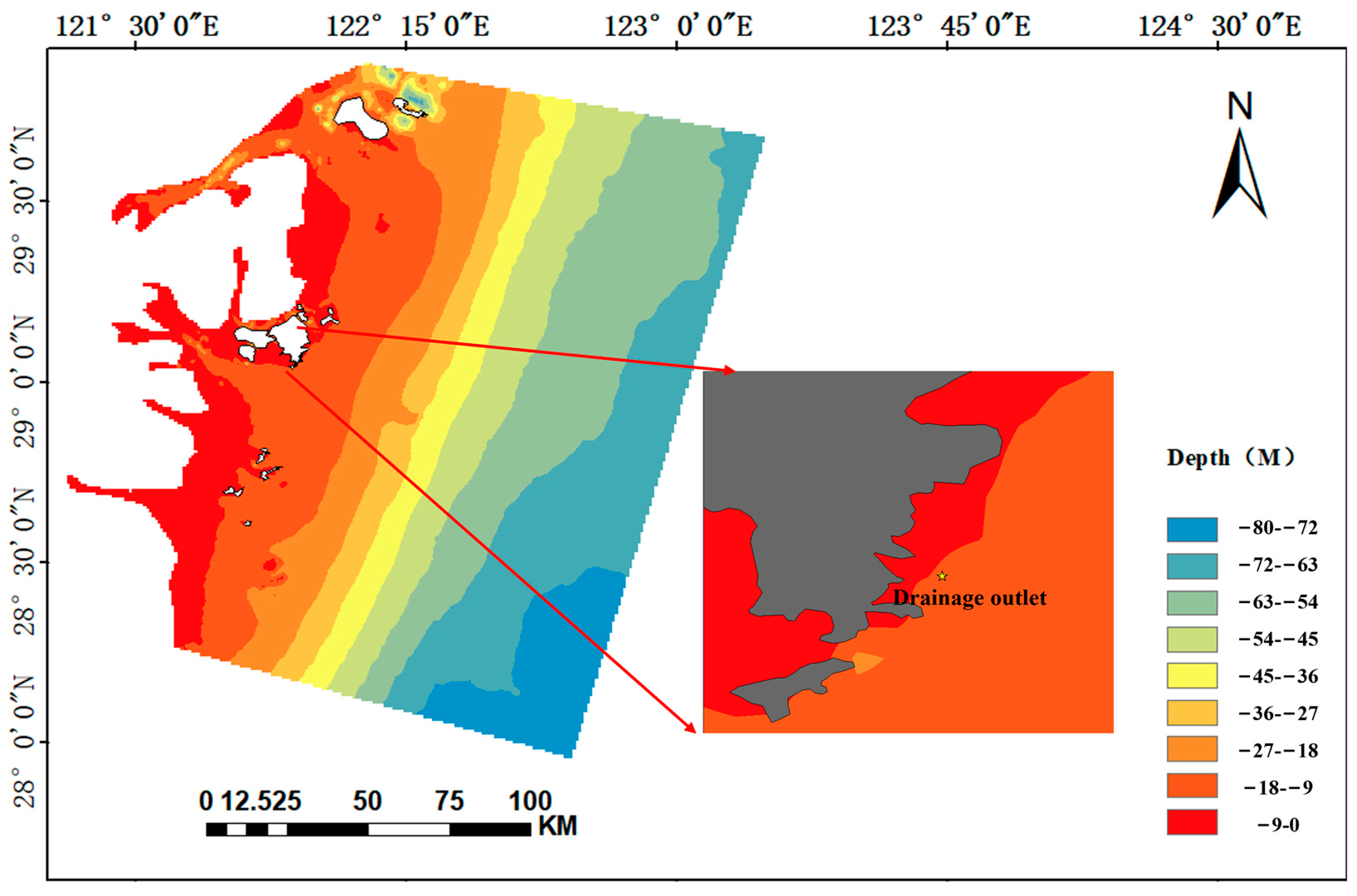
2.1. Overview of Study Area

The Jinqimen Nuclear Power Plant in Zhejiang is located on Nantian Island at the southern end of Xiangshan County, Ningbo City, Zhejiang Province, China. It faces Nanshan Island across the Jinqimen Waterway and is situated in the northern coastal waters at the mouth of Sanmen Bay, as shown in Figure 1. The model domain ranges from 121.25° E to 123.33° E in longitude and from 27.92° N to 30° N in latitude. This region, positioned at a relatively low latitude, belongs to the central subtropical zone and is characterized by a subtropical monsoon humid climate. It experiences distinct seasonal weather variations, due to alternating summer and winter monsoons, along with abundant rainfall throughout the year.
The surrounding environment contains a high density of sensitive areas. Within a 10 km radius of the plant site, there are critical zones including port and shipping areas, agricultural and fishery zones, and tourism and recreational areas. Therefore, accurate prediction and monitoring of thermal discharge from the Jinqimen Nuclear Power Plant are essential for ensuring environmental sustainability and mitigating potential ecological impacts.
The research on the Jinqimen Nuclear Power Plant began in 2015, with plans to construct six third-generation nuclear power units, all adopting “Hualong One” technology, which meets the highest international safety standards. Jinqimen Nuclear Power Plant is the largest advanced nuclear energy project in China. Once all six units are fully completed, the total installed capacity will reach approximately 7.2 million kilowatts, generating about 55 billion kilowatt–hours of electricity annually, which is equivalent to reducing carbon dioxide emissions by approximately 50 million tons.
The first phase of the power plant consists of two units, with a designed thermal discharge flow rate of 150 m3/s and a temperature rise of 8.2 °C.

2.2. Study Methodology

2.2.1. Model Introduction

MIKE 3 (2014) is a professional engineering software developed by the Danish Hydraulic Institute (DHI) for simulating three-dimensional free-surface flows. It effectively models non-uniform flows with different vertical density stratifications and can comprehensively account for external forces such as meteorological factors, tidal effects, and flow patterns, as well as other hydraulic conditions during the simulation process.
The MIKE 3 (2014) hydrodynamic model is based on the three-dimensional incompressible Navier–Stokes equations, which are time-averaged following the Reynolds-averaged theory and adhere to the Boussinesq assumption and the hydrostatic pressure assumption. The fundamental equations are expressed as follows [32]:
Continuity Equation:
u x + v y + w z = S
Momentum conservation equation:
(1)
Momentum Equation in the x-Direction:
u t + u 2 x + v u y + w u z = f v g ζ x 1 ρ 0 P a x g ρ 0 z ζ ρ x d z 1 ρ 0 h s x x x + S x y y + F u + z v t u z + u S S
(2)
Momentum Equation in the y-Direction:
v t + v 2 y + u v x + w v z = f u g ζ y 1 ρ 0 P a y g ρ 0 z ζ ρ y d z 1 ρ 0 h s y x x + S y y y + F v + z v t v z + v S S
In the above equations, t represents time (s); x, y, and z denote Cartesian coordinates; u, v, and w correspond to velocity components (m/s) in the x-, y-, and z-directions, respectively. The Coriolis parameter f is defined as f = 2Ω sin∅, where Ω represents the Earth’s angular velocity (rad/s) and ∅ denotes the geographical latitude (degrees). The water surface elevation is represented by ζ (m), while the total water depth h is calculated as h = ζ + d, where d indicates the distance (m) from the seabed to the still water level. The gravitational acceleration is denoted by g (m/s2).
The reference density of water is expressed as ρ 0 (kg/m3), with ρ representing the actual water density (kg/m3). Source and sink terms are collectively represented by S. The vertical eddy viscosity coefficient is denoted by v t . Atmospheric pressure is expressed as P a (kg/m·s2). Radiation stress components are represented by S x x , S x y , S y x , and S y y . The velocity components of source and sink terms are denoted by u s and v s , respectively.
F u and F v represent the horizontal stress terms, which can be expressed using the velocity gradient–stress relationship as follows:
F u = x 2 A u x + y A u y + v x
F v = x A u y + v x + y 2 A v y
In the aforementioned equations, A represents the horizontal eddy viscosity coefficient.
Temperature transport equation:
T t + u T x + v T y + w T z = z D v T z + x D h x + y D h y + H ^ + T s S
In the governing equations, x, y, and z represent the Cartesian coordinates. T denotes the water temperature, while D v signifies the vertical turbulent diffusion coefficient. S corresponds to the point source discharge rate, with t representing the temperature of the discharged effluent. The term Ĥ accounts for the temperature rise induced by heat flux across the free surface. F T represents the horizontal diffusion term for temperature, and D h denotes the horizontal diffusion coefficient.

2.2.2. Model Establishment

Based on the actual conditions of the engineering sea area, the model domain selected for this study centers around the waters where the Jinqimen Nuclear Power Plant is located. The southern boundary extends to the vicinity of Shitang Town, Wenling, the eastern boundary is set at the offshore −70 m isobath, the northern boundary reaches Chuanshan Peninsula in Beilun, Ningbo, and the upstream boundary of the Jiaojiang River extends to the upper reaches of Sanjiangkou.
A non-uniform triangular mesh was used for domain discretization. The maximum grid size in the open sea area is approximately 3.6 km, with gradually refined grids toward the project area. In particular, the mesh near the discharge outlet was further refined to ensure accurate simulation of temperature diffusion, migration, and high-temperature rise areas, with the smallest grid size set at approximately 20 m.
The model is vertically divided into three uniform layers, with the discharge outlet positioned at the bottom layer. The total number of mesh nodes in the computational domain is 30,515. The mesh configuration is shown in Figure 2.
The water depth data in the model consists of two sources. The bathymetric data for the waters near the power plant are obtained from depth data provided by the Navigation Guarantee Department of the Headquarters of the People’s Liberation Army Navy. For large-scale offshore areas, bathymetric data are derived from the ETOPO global topographic relief model provided by the U.S. National Geophysical Data Center (NGDC). Prior to interpolation, all data were uniformly processed to align with the mean sea level. The resulting bathymetric topography is shown in Figure 3.
To achieve a more accurate simulation of the flow field conditions in the project sea area, the model is driven using measured tidal level data. A key aspect of hydrodynamic numerical simulation is the determination of the stress, which is calculated using the following formula:
τ b ρ 0 = c f u b | u b |
In the governing equations, τ b represents the bottom shear stress (N/m2), while the bottom friction coefficient is denoted by c f (dimensionless). The near-bottom velocity vector u b = u b , v b is expressed in (m/s), and seawater density is represented by ρ 0 (kg/m3).
The magnitude of the bottom friction coefficient is primarily influenced by factors such as seabed sediment type, water depth, seabed topography, and vegetation. Based on the measured data and multiple model adjustments, the seabed roughness in the computational domain is set to 0.05 m.
In this study, the model was forced by water level data at the open boundary, which were predicted using the global tidal model TPXO9. It computed astronomical tides based on ten tidal constituents, namely M2, S2, K1, O1, N2, P1, K2, and Q1, along with the long-period constituents Mf and Mn. These constituents are generally capable of accurately representing the real astronomical tidal processes in the open boundary sea regions.
Additionally, parameters related to thermal discharge are configured in the model. Key parameters such as wind speed, air temperature, and sea surface temperature are derived from multiple summer observational datasets. The parameter values for the model’s temperature and salinity module are summarized in Table 1.

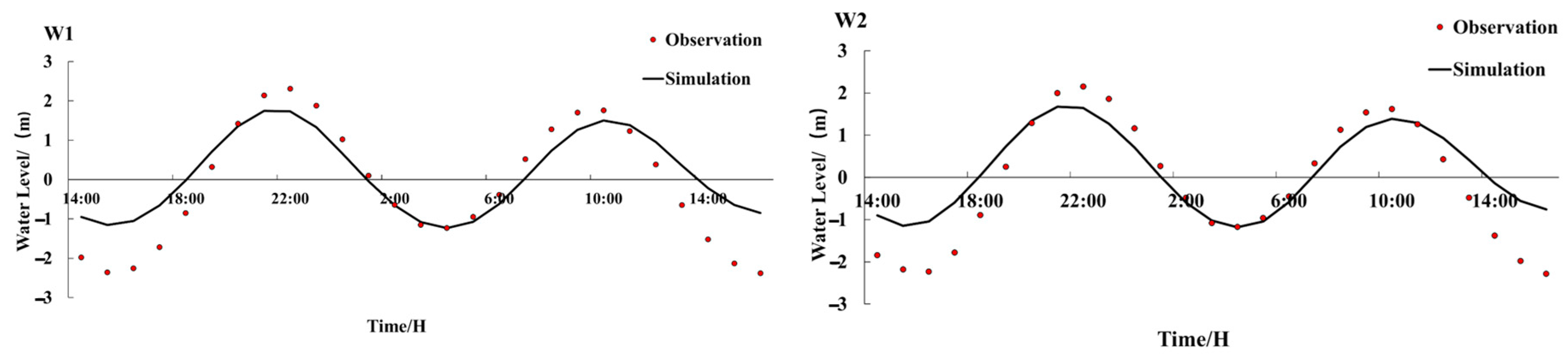
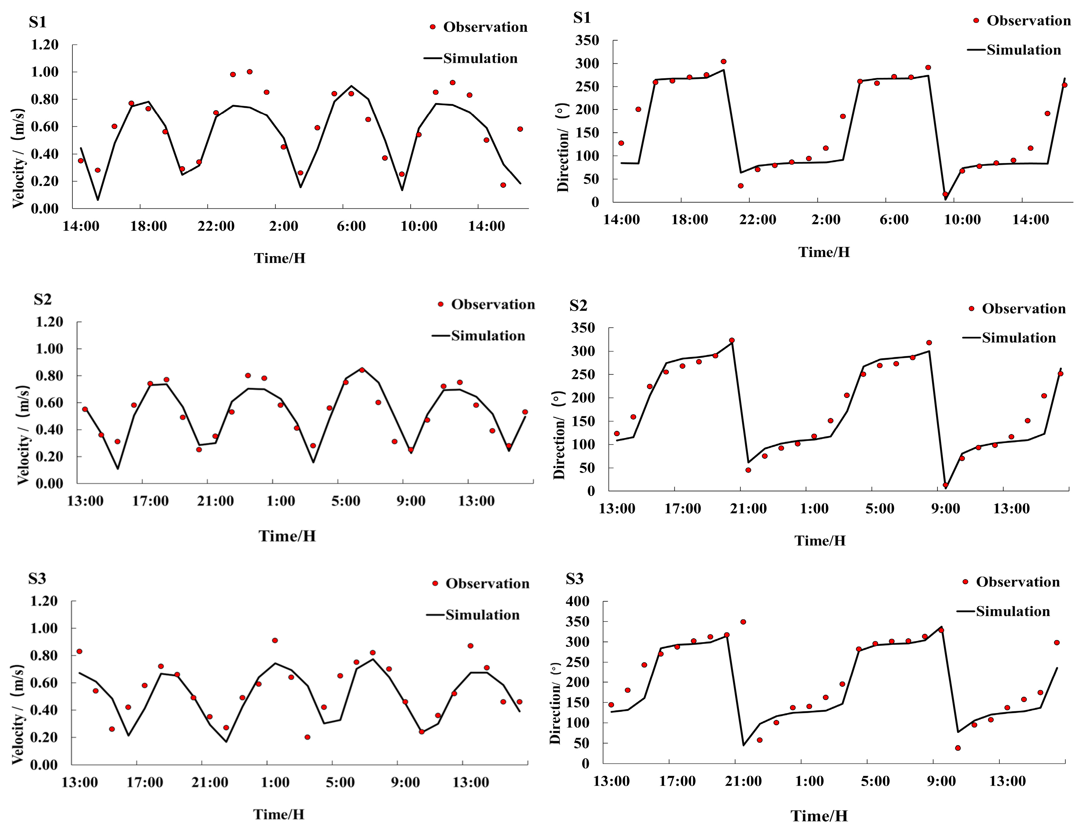
2.2.3. Model Verification

Model validation utilized measured data from survey stations during the spring tide period of 22–23 June 2020, with tidal level, current velocity, and current direction used as verification points. The comparisons between the model’s computational results and the measured data are shown in the following figures. Figure 4 presents the comparison between the simulated and observed tidal levels during the spring tide period, while Figure 5 illustrates the comparison between the simulated and observed current velocity and direction. From the figures, it can be seen that the model effectively captures the variations in current velocity and direction across different tidal cycles, demonstrating its capability for qualitative evaluation of hydrodynamic changes in the study area.
To quantitatively evaluate the accuracy of the hydrodynamic model simulation results, Willmott’s statistical method can be used for assessment [33]. The Willmott index of agreement is calculated using the following formula:
skill = 1 i = 1 n | M D | 2 i = 1 n ( | M D ¯ | + | D D ¯ | ) 2
In the validation metrics, M represents the model output while D denotes the observed data, with D ¯ indicating the mean value of the observations. The skill value, a dimensionless parameter ranging from 0 to 1, quantifies the correlation between the deviation of model predictions from the observed mean and the deviation of observations from their mean value, where a value of 1 indicates perfect agreement between model predictions and observations. Based on established evaluation criteria, model performance is classified as excellent when the skill value exceeds 0.65, very good for values between 0.65 and 0.5, good for values ranging from 0.5 to 0.2, and poor when the value falls below 0.2. The comprehensive validation results, which demonstrate the model’s predictive capability across various metrics, are systematically presented in Table 2 for detailed analysis and comparison with the observational data.
Through the above qualitative and quantitative analyses, the developed numerical model accurately reflects the hydrodynamic characteristics of the Jinqimen Nuclear Power Plant region. Based on this validated model, further research on the feasibility study and three-dimensional numerical simulation of recirculating cooling water thermal discharge for the Zhejiang Jinqimen Nuclear Power Plant can be conducted.

2.2.4. Operating Conditions Design

To investigate the impact of changing the jet angle on the temperature rise at the intake, this study modified both the jet angle and jet velocity. The jet angle was set to six different conditions (free diffusion, 0°, 30°, etc.), while the jet velocity was set to two values (0 m/s and 1.12 m/s, where 1.12 m/s represents the design velocity). This results in a total of six operating conditions. The specific settings are detailed in Table 3.

3. Results and Discussion

3.1. Hydrodynamic Field Characterization and Analysis

Figure 6 illustrates the hydrodynamic model results during peak flood and peak ebb tides under spring tide conditions in the summer of 2020. During peak flood tide, the tidal current in the northeastern waters of the plant site predominantly flows southwestward along the coast. After converging with the northwestward flow from the southwestern waters of the plant site, the overall current direction shifts northwestward. In the eastern section of the Jinqimen Waterway, the local tidal current velocity slightly decreases. Upon entering Nantian Bay, the flow is constrained by the narrowing topography, causing an increase in velocity. The maximum flood tide velocity is observed southwest of Nanshan Island. During peak ebb tide, as the tidal current flows out of Nantian Bay, its velocity increases. The Jinqimen Waterway enhances the flow velocity in the eastern local sea area, but the current speed decreases as it moves further northward, forming an overall northeastward coastal flow. In the waters surrounding the plant site, the western side exhibits higher current velocities than the eastern side. The study area is dominated by rectilinear tidal currents, a topographic forcing-induced regime where flood and ebb currents exhibit opposed or nearly opposed flow directions. Notably, flood tidal currents demonstrate significantly greater flow velocities compared to ebb currents in this region.
Residual currents refer to the remaining flow after filtering out periodic tidal currents and include components such as wind-driven currents, density currents, runoff, and tidal residual currents. Among these, tidal residual currents differ significantly from the other components, as their generation mechanism remains relatively stable over long time scales and continuously contributes to the overall residual flow. Tidal residual currents play a crucial role in the transport of substances in seawater, such as heat, dissolved salts, pollutants, and nutrients. Therefore, studying the residual current field is essential for understanding thermal diffusion processes. Figure 7 presents the residual current patterns near the project area under different jet angles, demonstrating six distinct operational scenarios. The residual currents predominantly exhibit a southwestward coastal flow pattern across all cases. The primary variations among scenarios manifest in the flow field characteristics near the discharge outlet. In Scenario 1, the thermal discharge shows relatively weaker residual currents at the outlet due to the absence of initial jet velocity. Scenario 2 is characterized by an eastward cross-flow at the discharge point. Scenario 3 displays a distinct surface layer flow pattern. Scenarios 4 through 6 reveal a gradual transition in flow direction at the discharge outlet, evolving from eastward to vertically surface layer orientation with increasing velocity magnitude.

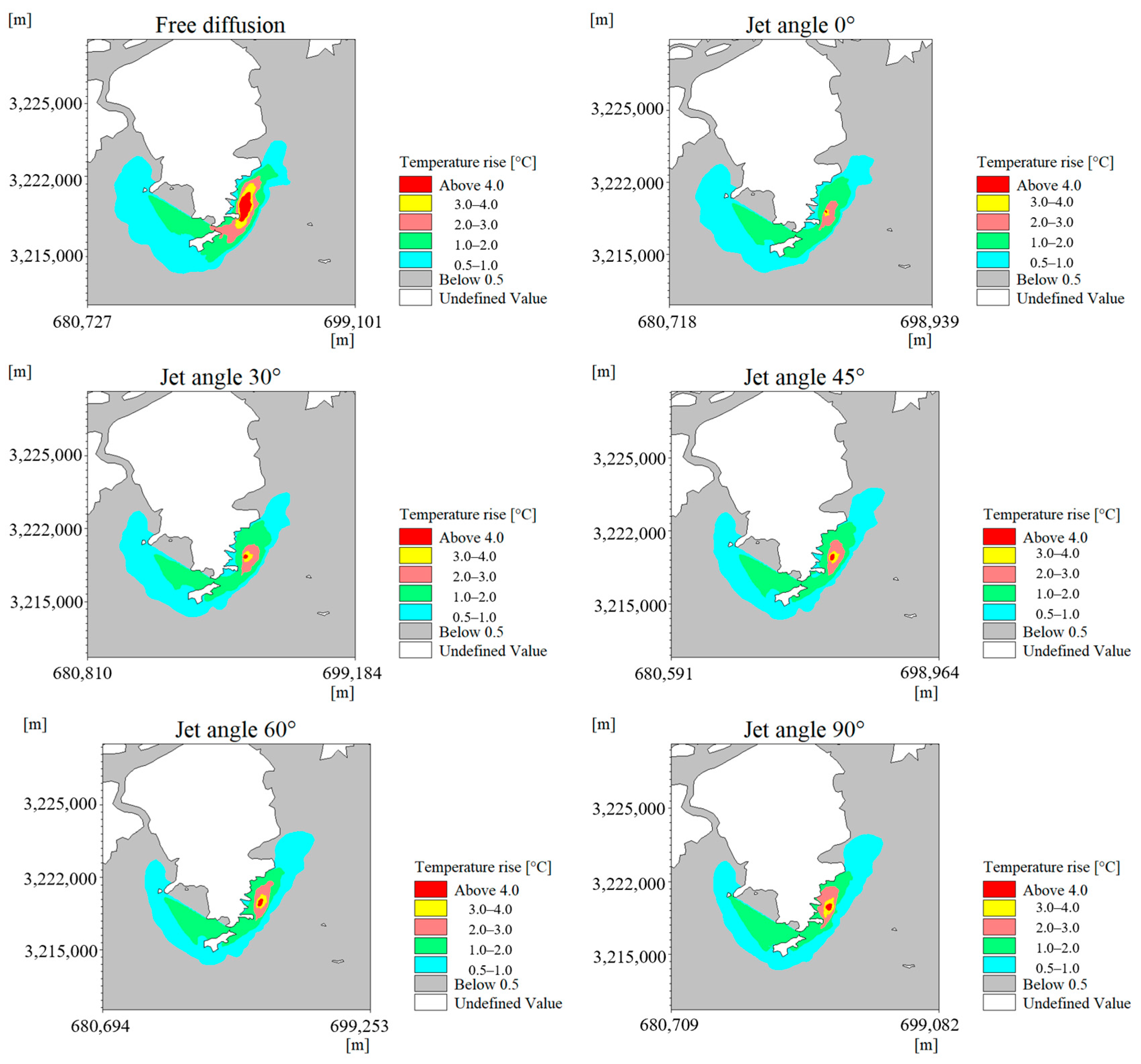
3.2. Analysis of Temperature Rise Results

Considering the influence of initial conditions on temperature rise results while ensuring model stability, this study extracted simulation results from the 15th day of model operation for temperature rise calculations. The maximum thermal rise envelope area at different temperature rise stages was projected vertically and analyzed. The maximum thermal rise envelope areas are presented in Table 4.
From Table 4, it can be observed that the maximum temperature rise envelope area predominantly occurs at the surface layer across all scenarios. This phenomenon is due to changes in water density—heated surface water becomes denser and begins to sink, while lighter bottom water rises, facilitating thermal mixing. Scenario 2, which includes an initial jet velocity, exhibits its largest thermal rise envelope area at the bottom layer. Scenario 1, characterized by free diffusion, consistently exhibits the largest temperature rise envelope areas across all thermal rise stages. As the discharge outlet angle increases, the high-temperature rise (4 °C) envelope area gradually expands, while the low-temperature rise (0.5 °C) envelope area progressively decreases.
These findings indicate that discharge angle adjustments play a crucial role in the spatial distribution of thermal dispersion, affecting both the extent and depth of temperature rise in the receiving waters.
Figure 8 presents the maximum thermal rise envelope area in vertical projection for the six scenarios, providing a clearer visualization of the temperature diffusion patterns across different conditions. Across all scenarios, the thermal discharge exhibits a southwestward diffusion trend. Under the summer neap tide hydrodynamic conditions, the tidal current near the discharge outlet flows predominantly southwestward along the coast during flood tide and northeastward during ebb tide. Consequently, the thermal discharge is transported and dispersed in both the northeastward and southwestward directions. Notably, the overall current velocity is higher on the western side of the study area compared to the eastern side, and the residual flow is primarily southwestward. As a result, the thermal rise boundary experiences stronger transport intensity toward the southwest. These findings highlight the influence of regional hydrodynamics on the spatial dispersion of thermal discharge, which is crucial for optimizing discharge outlet placement and minimizing environmental impact.
From Table 4 and Figure 8, it is evident that a thermal stratification phenomenon occurs in the high-temperature rise zone near the discharge outlet, where the surface layer exhibits a larger high-temperature area than the bottom layer. As the distance from the discharge outlet increases, the thermal discharge is gradually diluted by the surrounding water, leading to temperature reduction and a weakening of buoyancy effects. Consequently, thermal mixing in the vertical direction becomes more uniform, and the differences in distribution patterns and area among different layers in the low-temperature rise zone gradually diminish.
This study identifies that Scenario 3, with a discharge jet angle of 30°, exhibits the smallest thermal rise envelope area, indicating strong dilution, transport, and diffusion capacity. Under this configuration, heat does not accumulate easily, making it the most effective setup for minimizing localized thermal pollution.

3.3. Environmental Sensitive Areas

Figure 9 presents the vertical projection analysis of thermal discharge dispersion under Scenario 3 superimposed with environmentally sensitive areas, revealing that the 1 °C temperature rise affects both the northern and western aquaculture area along with the northern leisure tourist areas, while higher temperature rises (2–4 °C) show progressively more concentrated impacts on northern leisure tourist areas. These findings underscore the need for focused environmental monitoring in these sensitive areas. Historical studies since the 1970s have demonstrated the dual nature of thermal discharge effects, showing its beneficial applications in aquaculture through reduced climatic dependence, extended growth periods, and enhanced production yields, while simultaneously highlighting the critical need for stringent temperature monitoring in high-impact areas, strict emission controls, and maintenance of ecosystem protection thresholds. This analysis emphasizes the importance of implementing balanced management strategies that capitalize on the productive uses of thermal discharge while rigorously enforcing comprehensive temperature regulation measures to prevent ecological boundary violations and protect sensitive marine environments.
In compliance with China’s Marine Thermal Discharge Regulations, a 4 °C temperature rise serves as the operational threshold for coastal water usage. When the 4 °C thermal plume intrudes into ecologically sensitive zones (particularly aquaculture areas and tourist destinations), the discharge scheme warrants a thorough environmental assessment. Our comparative analysis reveals that Case 3 demonstrates the minimal spatial extent of 4 °C temperature increase within sensitive areas, representing the most environmentally favorable configuration among all evaluated scenarios.

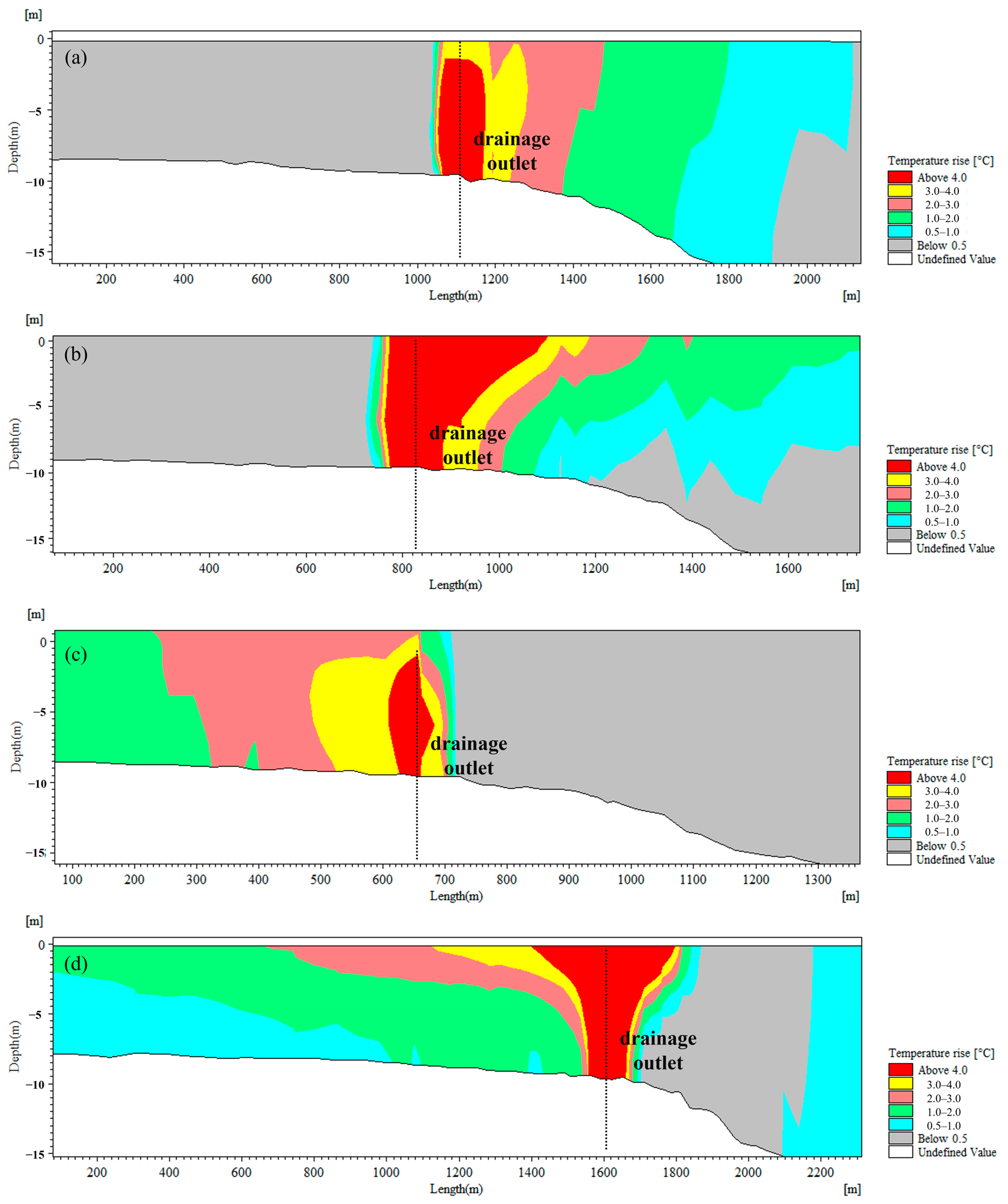
3.4. Vertical Diffusion of Thermal Discharge

Taking Scenario 1, which exhibits the largest thermal rise envelope area, as an example, we investigate the relationship between depth, flow velocity, and temperature rise. A longitudinal section along the flow direction, including the discharge outlet, was selected at four tidal phases: peak flood tide, slack high tide, peak ebb tide, and slack low tide. Temperature rise and depth were extracted and compared, with the results shown in Figure 10.
From Figure 10, the following patterns are observed: During peak flood tide and peak ebb tide, the thermal dispersion exhibits a strip-like pattern, with the high-temperature rise zone concentrated at the bottom layer. During slack high tide and slack low tide, the thermal dispersion appears wider at the top and narrower at the bottom, with the high-temperature rise zone primarily located at the surface layer. At peak flood and ebb tides, strong tidal dynamics enhance thermal diffusion, resulting in a smaller high-temperature rise area due to efficient mixing. At slack high and low tides, weaker tidal forces cause thermal accumulation, leading to a larger high-temperature rise area as heated water stagnates.
These findings indicate that tidal dynamics play a crucial role in regulating thermal discharge dispersion, with strong currents enhancing heat dissipation and weak currents promoting heat accumulation in the receiving water body.
This study employs a three-dimensional baroclinic model, which provides a more accurate representation of thermal stratification. The results are consistent with the findings of Zhang et al. [24] using the MIKE 3 (2014) temperature–salinity module, confirming that surface current velocity is greater than bottom current velocity. Due to thermal buoyancy, the discharged warm water rises to the surface, where the faster surface currents lead to a larger temperature dispersion range compared to the bottom layer.

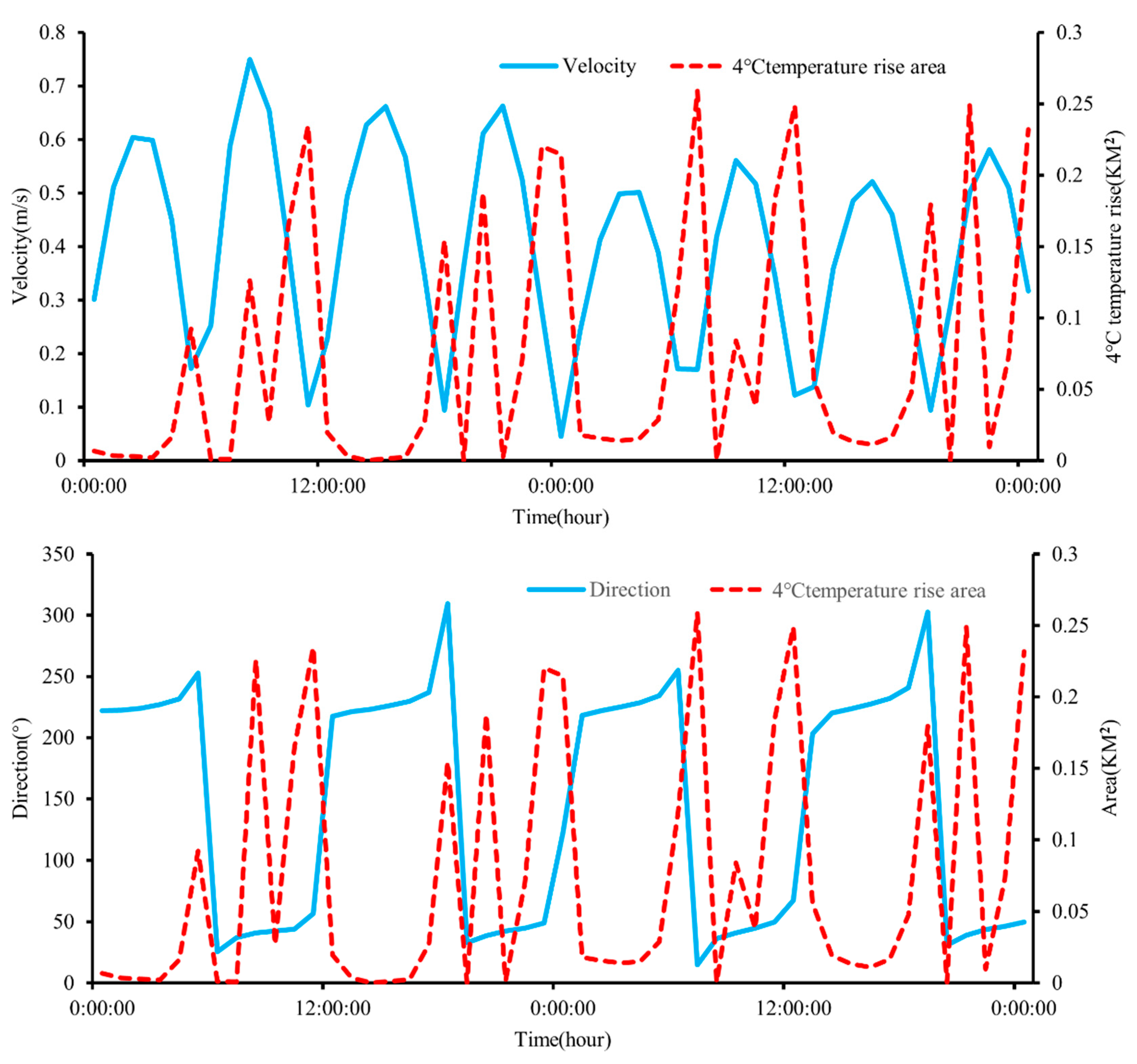
3.5. Temperature Rise Area and Tidal Current

To further quantify the impact of tidal currents on the thermal discharge dispersion at the Jinqimen Nuclear Power Plant, the correlation coefficients between surface thermal rise area and tidal currents (speed and direction) were calculated, as shown in Figure 11. The analysis reveals a general negative correlation between surface thermal rise area and spring tide currents, with correlation coefficients of R = −0.56 (flow speed) and R = −0.49 (flow direction). These results indicate that strong tidal currents induce significant vertical mixing, which inhibits horizontal dispersion of thermal discharge in offshore waters. This finding aligns with previous research by Geng et al. [19], further validating the influence of tidal dynamics on thermal pollution dispersion.
The study results indicate that thermal discharge from nuclear power plants undergoes significant dispersion upon entering the receiving water body, leading to distinct thermal stratification. This phenomenon has also been observed in previous research by scholars such as Parshakova et al. [34] and Zhou et al. [35]. Additionally, our findings highlight that tidal effects play a crucial role in coastal nuclear power plant thermal discharge dynamics.
Furthermore, Zhao et al. [36] discovered that the growth of N. oceanica is not directly correlated with temperature rise but is more influenced by vertical displacement caused by tidal movement. Therefore, understanding the role of tides in driving thermal discharge is essential for better comprehending thermal diffusion in marine environments and evaluating its ecological impacts.

3.6. Summary and Future Work

In summary, this study reveals thermal stratification characteristics of thermal discharge in marine environments and investigates the effects of different jet angles on thermal dispersion. The results are consistent with previous research, demonstrating that this study provides a scientific reference for the regulation and management of thermal discharge at the Jinqimen Nuclear Power Plant.
In future studies, the simulation scope will be expanded by incorporating tidal dynamics during the winter season to better capture seasonal variability. In addition, quantitative analyses and risk threshold assessments for environmentally sensitive areas will be enhanced, thereby enabling the provision of more comprehensive recommendations for nuclear power plant development.

4. Conclusions

This study, using the Jinqimen Nuclear Power Plant in Zhejiang Province, China, as a case study, systematically analyzed the thermal dispersion characteristics of thermal discharge under different jet angles through three-dimensional numerical simulations validated with field data. The main conclusions are as follows:
Jet angle significantly influences the temperature rise distribution: Under free diffusion conditions, the temperature rise area is largest, with the high-temperature rise zone concentrated at the surface. Increasing the jet angle (from 0° to 90°) reduces the low-temperature rise area but expands the high-temperature rise area. The 30° jet angle condition performs optimally in reducing the temperature rise area and enhancing heat dilution capacity.
Thermal stratification occurs in the high-temperature rise zone near the discharge outlet: The surface layer exhibits a larger high-temperature rise area than the bottom layer. As the distance from the discharge outlet increases, thermal discharge is diluted by ambient water, leading to temperature reduction and weaker buoyancy effects. The vertical mixing of thermal discharge becomes more uniform, and differences in temperature rise distribution across layers diminish.
The thermal field of the Jinqimen Nuclear Power Plant is influenced by tidal dynamics in the engineering sea area: The region experiences complex tidal dynamics, with stronger currents on the western side of the plant compared to the eastern side. The residual current flows southwestward along the coast. During the summer neap tide of 2020, thermal discharge diffused in both northeastward and southwestward directions, with stronger transport and dispersion toward the southwest.
Engineering Implications: The findings provide theoretical support for optimizing nuclear power plant discharge outlet designs. It is recommended that a 30° jet angle be prioritized in practical engineering applications to enhance thermal dispersion efficiency.
Future studies should integrate a wider range of jet angle parameters, seasonal hydrodynamic variations, and ecological response models to comprehensively evaluate the long-term environmental impact of thermal discharge.

Author Contributions

Methodology, L.L. and H.S.; Software, L.L. and H.X.; Formal analysis, L.L., H.S. and C.Z.; Resources, Q.W.; Data curation, L.L.; Writing—original draft, L.L.; Writing—review & editing, H.S. and C.Z.; Supervision, H.X.; Funding acquisition, Q.W. and C.Z. All authors have read and agreed to the published version of the manuscript.

Funding

The authors declare that financial support was received for the research, authorship, and/or publication of this article. This research was supported by the National Key R&D Program of China (2023YFC3007900, 2023YFC3007905), the National Natural Science Foundation Key Project (42330406, 42476163), and the Yantai Science and Technology Innovation Project (2023JCYJ094).

Data Availability Statement

Data are contained within the article.

Conflicts of Interest

The authors declare no conflict of interest.

References

  1. Okunev, V.S. Prospects for the development of the concept of a safe nuclear reactor BREST of maximum limiting power for nuclear energetics of the middle of the XXI century. In IOP Conference Series: Materials Science and Engineering; IOP Publishing: Bristol, UK, 2021; Volume 1100, p. 012002. [Google Scholar]
  2. Ye, Y.; Chen, K.; Zhou, Q.; Xiang, P.; Huo, Y.; Lin, M. Impacts of thermal discharge on phytoplankton in Daya Bay. J. Coast. Res. 2018, 83, 135–147. [Google Scholar] [CrossRef]
  3. Bozorgchenani, A.; Seyfabadi, J.; Shokri, M.R. Effects of thermal discharge from Neka power plant (southern Caspian Sea) on macrobenthic diversity and abundance. J. Therm. Biol. 2018, 75, 13–30. [Google Scholar] [CrossRef]
  4. Li, X.Y.; Li, B.; Sun, X.L. Effects of a coastal power plant thermal discharge on phytoplankton community structure in Zhanjiang Bay, China. Mar. Pollut. Bull. 2014, 81, 210–217. [Google Scholar] [CrossRef] [PubMed]
  5. Huang, X.N.; Zhu, Z.H.; Xu, M.C.; Jing, Q. Variation of water temperature in the southwestern Daya Bay before and after the operation of Daya Bay nuclear power plant. In Annual Research Reports (II): Marine Biology Research Station at Daya Bay; Science Publishing House: Beijing, China, 1998; pp. 102–112. [Google Scholar]
  6. Barnett, P.R.O. Some changes in intertidal sand communities due to thermal pollution. Proc. R. Soc. Lond. Ser. B Biol. Sci. 1971, 177, 353–364. [Google Scholar]
  7. Vinnå, L.R.; Wüest, A.; Bouffard, D. Physical effects of thermal pollution in lakes. Water Resour. Res. 2017, 53, 3968–3987. [Google Scholar] [CrossRef]
  8. Min, S.H.; Lim, S.Y.; Yoo, S.H. The environmental benefits of reducing thermal discharge from nuclear power generation. Energy Environ. 2017, 28, 885–894. [Google Scholar] [CrossRef]
  9. Zeng, Z.; Luo, Y.; Chen, Z.; Tang, J.; Wang, Y.; Chen, C. Impact assessment of thermal discharge from the Kemen power plant based on field observation and numerical simulation. J. Coast. Res. 2020, 104, 351–361. [Google Scholar] [CrossRef]
  10. Ardalan, H.; Vafaei, F. Hydrodynamic classification of submerged thermal-saline inclined single-port discharges. Mar. Pollut. Bull. 2018, 130, 299–306. [Google Scholar] [CrossRef]
  11. Liu, M.; Yin, X.; Xu, Q.; Chen, Y.; Wang, B. Monitoring of fine-scale warm drain-off water from nuclear power stations in the Daya Bay based on Landsat 8 data. Remote Sens. 2020, 12, 627. [Google Scholar] [CrossRef]
  12. George, A.M. Numerical Simulation of Warm Discharge in Cold Fresh Water. Doctoral Dissertation, Loughborough University, Loughborough, UK, 2017. [Google Scholar]
  13. Templeton, W.L.; Schneider, M.J.; Gibson, C.I. Effects of Thermal and Chemical Discharges from Nuclear Power Plants; (No. BNWL-SA-5206; CONF-741137-1); Battelle Pacific Northwest Labs.: Richland, WA, USA, 1974. [Google Scholar]
  14. Zhang, X.; Jia, S.; Zhang, S.; Pei, L.; Liu, Y. Research and application of real-time monitoring buoy system for marine water temperatures of vertical profiles. Ocean Sci. 2016, 5, 109–114. [Google Scholar]
  15. Wang, L.; Li, G.; Shi, H.; Zhu, J.; Zhan, C.; Zhang, X.; Wang, Q. Integrated monitoring and prediction of thermal discharge from nuclear power plants using satellite, UAV, and numerical simulation. Environ. Monit. Assess. 2024, 196, 736. [Google Scholar] [CrossRef] [PubMed]
  16. Huang, W.; Jiao, J.; Zhao, L.; Hu, Z.; Peng, X.; Yang, L.; Chen, F. Thermal discharge temperature retrieval and monitoring of NPPs based on SDGSAT-1 images. Remote Sens. 2023, 15, 2298. [Google Scholar] [CrossRef]
  17. Dai, X.; Guo, Z.; Lin, Y.; Wei, C.; Ye, S. Application of satellite remote sensing data for monitoring thermal discharge pollution from Tianwan nuclear power plant in eastern China. In Proceedings of the 2012 5th International Congress on Image and Signal Processing, Chongqing, China, 16–18 October 2012; IEEE: New York, NY, USA; pp. 1019–1023. [Google Scholar]
  18. Ge, X.; Zhao, Y.; Yuan, J.; Liu, J.; Cao, Y. Experimental Study on Thermal Effluent of a Coastal Nuclear Power Plant With Outlet-intake Project Layout. Adv. Mar. Sci. 2015, 33, 512–519. [Google Scholar]
  19. Geng, B.; Lu, L.; Cao, Q.; Zhou, W.; Li, S.; Wen, D.; Hong, M. Three-dimensional numerical study of cooling water discharge of Daya Bay Nuclear Power Plant in southern coast of China during summer. Front. Mar. Sci. 2023, 9, 1012260. [Google Scholar] [CrossRef]
  20. Huang, F.; Lin, J.; Zheng, B. Effects of thermal discharge from coastal nuclear power plants and thermal power plants on the thermocline characteristics in sea areas with different tidal dynamics. Water 2019, 11, 2577. [Google Scholar] [CrossRef]
  21. Wang, S.; Chen, F.; Zhang, W. Numerical investigation of temperature distribution of thermal discharge in a river-Type reservoir. Pol. J. Environ. Stud. 2019, 28, 3909–3917. [Google Scholar] [CrossRef]
  22. Ma, J.R.; Guo, Y.Q. Effect of Initial Grid’s Size in Thermal Diffusion Simulation. Adv. Mater. Res. 2012, 516, 512–518. [Google Scholar] [CrossRef]
  23. Durán-Colmenares, A.; Barrios-Piña, H.; Ramírez-León, H. Numerical modeling of water thermal plumes emitted by thermal power plants. Water 2016, 8, 482. [Google Scholar] [CrossRef]
  24. Zhang, X.; Shi, H.; Zhan, C.; Zhu, J.; Wang, Q.; Li, G. Numerical simulation calculation of thermal discharge water diffusion in coastal nuclear power plants. Atmosphere 2023, 14, 1371. [Google Scholar] [CrossRef]
  25. Gaeta, M.G.; Samaras, A.G.; Archetti, R. Numerical investigation of thermal discharge to coastal areas: A case study in South Italy. Environ. Model. Softw. 2020, 124, 104596. [Google Scholar] [CrossRef]
  26. Laguna-Zarate, L.; Barrios-Piña, H.; Ramírez-León, H.; García-Díaz, R.; Becerril-Piña, R. Analysis of thermal plume dispersion into the sea by remote sensing and numerical modeling. J. Mar. Sci. Eng. 2021, 9, 1437. [Google Scholar] [CrossRef]
  27. Lee, M.E.; Lee, J.; Al-Osairi, Y. Study on the local sea water temperature variation for the industrial water use of Al-Zour coastal area in Kuwait. Desalin. Water Treat. 2020, 176, 9–17. [Google Scholar] [CrossRef]
  28. Cheng, Y.; Wu, K. Study on Submerged Type of Thermal Discharge in Power Plant by Using Numerical Similation. J. North China Electr. Power Univ. Nat. Sci. Ed. 2016, 43, 88–94. [Google Scholar]
  29. Yan, Z.; Dao-zeng, W.; Jing-yu, F. Experimental investigations on diffusion characteristics of high concentration jets in environmental currents. Appl. Math. Mech. 2002, 23, 1429–1436. [Google Scholar] [CrossRef]
  30. Zhang, C.; Yao, J.; Tao, J. Advances in numerical simulation of thermal discharge of heat or nuclear power plants in coastal areas. Adv. Sci. Technol. Water Resour. 2010, 30, 84–88. [Google Scholar]
  31. Yao, P.; Xue, Q.; Lu, H.; Zhang, E. Current status and prospects of nuclear power plant thermal discharge monitoring technology. World Nucl. Geosci. 2025. [Google Scholar] [CrossRef]
  32. Chen, Y.; Ma, Q.Y.; Liu, C.; Shu, Q.; Rashid, H. Research on the impact of reclamation project on surrounding water environment. Desalin. Water Treat. 2021, 219, 77–83. [Google Scholar] [CrossRef]
  33. Willmott, C.J. On the validation of models. Phys. Geogr. 1981, 2, 184–194. [Google Scholar] [CrossRef]
  34. Parshakova, Y.N.; Lyubimova, T.P. Computer modelling of technogenic thermal pollution zones in large water bodies. J. Phys. Conf. Ser. 2018, 955, 012017. [Google Scholar] [CrossRef]
  35. Zhou, Q.J. A three-dimensional numerical simulation of thermal discharge in daya bay. Trans. Oceanol. Limnol. 2007, 4, 37–46. [Google Scholar]
  36. Zhao, Y.J.; Zeng, L.; Zhang, A.L.; Wu, Y.H. Response of current, temperature, and algae growth to thermal discharge in tidal environment. Ecol. Model. 2015, 318, 283–292. [Google Scholar] [CrossRef]
Figure 1. Geographic location of the study area, hydrological observation points, and discharge outlet positions.
Jmse 13 00931 g001
Figure 2. Model grid configuration.
Jmse 13 00931 g002
Figure 3. Bathymetric map of the Jinqimen model.
Jmse 13 00931 g003
Figure 4. Comparison of simulated and measured tidal levels.
Jmse 13 00931 g004
Figure 5. Comparison of simulated and measured current velocity and direction.
Jmse 13 00931 g005
Figure 6. Flow field conditions in the engineering area: (left) Ebb tide flow field; (right) flood tide flow field.
Jmse 13 00931 g006
Figure 7. Residual current diagrams of different jet angles (unit: m/s).
Jmse 13 00931 g007
Figure 8. Envelope area of maximum temperature rise in vertical projection.
Jmse 13 00931 g008
Figure 9. Distribution of sensitive areas near the factory site.
Jmse 13 00931 g009
Figure 10. Vertical diffusion of temperature rise: (a) Flood peak; (b) high slack water; (c) ebb peak; (d) low slack water.
Jmse 13 00931 g010
Figure 11. Comparison of the area of temperature rise and tidal current during the major tidal surge period (00:00 5–7 July 2020).
Jmse 13 00931 g011
Table 1. Key parameter settings of the model.
Key ParameterValue
Laten heat20 W/m2 °C
Sensible heat12 W/m2 °C
Short wave radiation−17 W/m2 °C
Long wave radiation30 W/m2 °C
Air temperature32 °C
Sea surface temperature30 °C
Wind speed at 1.5 m above sea level3.32 m/s
Design temperature rise8.2 °C
Table 2. Model evaluation results.
Stations NameEvaluation ItmesSkill ValueEvaluation Results
W1Water level0.7Excellent
W20.7Excellent
S1Flow velocity0.8Excellent
Flow direction1Excellent
S2Flow velocity0.9Excellent
Flow direction1Excellent
S3Flow velocity0.9Excellent
Flow direction0.9Excellent
Table 3. Operating conditions design.
Operating ConditionsJet Angle (°)Jet Speeds (m/s)Outlet Location (m)
Operating Conditions 1Free Diffusion0−7.5
Operating Conditions 21.12−7.5
Operating Conditions 330°1.12−7.5
Operating Conditions 445°1.12−7.5
Operating Conditions 560°1.12−7.5
Operating Conditions 690°1.12−7.5
Table 4. Temperature rise area for different jet angles.
Jet Angles Temperature Rise Area (km2)
0.5 (°C)1 (°C)2 (°C)3 (°C)4 (°C)
Free DiffusionSurface layer47.5217.755.892.621.31
Middle layer44.0012.160.550.230.13
bottom layer41.478.530.170.090.05
Projection plane47.5217.825.892.621.31
Surface layer40.1614.831.290.020.00
Middle layer38.2212.530.720.090.01
bottom layer37.8712.100.640.100.02
Projection plane40.6814.971.320.130.03
30°Surface layer36.7313.641.740.340.07
Middle layer35.9012.400.830.110.03
bottom layer34.9911.170.380.050.01
Projection plane37.0313.641.760.350.07
Jet Angles Temperature Rise Area (km2)
0.5 (°C)1 (°C)2 (°C)3 (°C)4 (°C)
45°Surface layer35.5113.841.940.400.11
Middle layer35.0312.811.040.210.06
bottom layer34.2111.010.420.070.01
Projection plane35.6813.841.940.400.11
60°Surface layer36.2213.682.160.540.15
Middle layer35.8212.901.330.330.08
bottom layer35.0611.570.670.140.01
Projection plane36.5113.732.160.540.15
90°Surface layer35.7913.842.570.670.16
Middle layer35.3113.001.750.380.09
bottom layer34.5011.880.700.160.01
Projection plane35.9213.942.570.670.16
Disclaimer/Publisher’s Note: The statements, opinions and data contained in all publications are solely those of the individual author(s) and contributor(s) and not of MDPI and/or the editor(s). MDPI and/or the editor(s) disclaim responsibility for any injury to people or property resulting from any ideas, methods, instructions or products referred to in the content.

