Article

An AIS-Based Study to Estimate Ship Exhaust Emissions Using Spatio-Temporal Approach

1
Department of Maritime AI & Cyber Security, Graduate School of National Korea Maritime & Ocean University, Busan 49112, Republic of Korea
2
Research Institute of Medium & Small Shipbuilding, Changwon 51965, Republic of Korea
3
Division of Maritime AI & Cyber Security, National Korea Maritime & Ocean University, Busan 49112, Republic of Korea
*
Author to whom correspondence should be addressed.
J. Mar. Sci. Eng. 2025, 13(5), 922; https://doi.org/10.3390/jmse13050922
Submission received: 7 April 2025 / Revised: 30 April 2025 / Accepted: 3 May 2025 / Published: 7 May 2025

Abstract

:
The global shipping industry facilitates the movement of approximately 80% of goods across the world but accounts for nearly 3% of total greenhouse gas (GHG) emissions every year, and other pollutants. One challenge in reducing shipping emissions is understanding and quantifying emission characteristics. A detailed method for calculating shipping emissions should be applied when preparing exhaust gas inventory. This research focused on quantifying CO2, NOx, and SOx emissions from tankers, containers, bulk carriers, and general cargo in the Republic of Korea using spatio-temporal analysis and maritime big data. Using the bottom-up approach, this study calculates vessel emissions from the ship engines while considering the fuel type and operation mode. It leveraged the Geographic Information System (GIS) to generate spatial distribution maps of vessel exhausts. The research revealed variability in emissions according to ship types, sizes, and operational modes. CO2 emissions were dominant, totaling 10.5 million tons, NOx 179,355.2 tons, and SOx 32,505.1 tons. Tankers accounted for about 43.3%, containers 33.1%, bulk carriers 17.3%, and general cargo 6.3%. Further, emissions in hoteling and cruising were more significant than during maneuvering and reduced speed zones (RSZs). This study contributes to emission databases, providing a basis for the establishment of targeted emission control policies.

1. Introduction

Maritime transportation plays a vital role in the development of global trade and economic growth. However, it is also a remarkable contributor to atmospheric pollution [1]. Approximately 90% of the global trade volume is carried by ship, leading to high volumes of exhaust emissions, which have negative impacts [2]. The Second International Maritime Organization (IMO) Greenhouse Gas study [3] suggests that shipping greenhouse emissions accounted for approximately 3.3% of global emissions, with projections indicating a continued rise if mitigation strategies are not intensified. In the IMO GHG study, carbon dioxide was the highest emitted greenhouse gas in terms of quantity and global warming potential. A ship’s engine combustion emits 450 different air pollutants [4], but the key ship sources of air pollutants are greenhouse gases, carbon monoxide, NOx, SOx, and particulate matter [5,6]. Around 70% of these vessel emissions are discharged within a radius of 400 km from the coastline, and the emissions travel further through the atmosphere as ships maneuver near densely inhabited coastal areas [7]. As a result, around 230 million people living in the top 100 world ports are directly impacted by marine pollution [8].
To address this, international bodies such as the IMO have set increasingly ambitious targets. The IMO, through its legislation, the International Convention on the Prevention of Pollution from Ships (MARPOL) Annex VI, has regulations to mitigate maritime pollution. Since 2018, the IMO has actively analyzed shipping emissions to establish long-term strategies to control marine pollution, including the IMO 2020 sulfur limit [9]. In the NOx ECAs, tiered emission limits are imposed based on the ship’s engine construction date and type. Carbon dioxide is one of the largest contributors to global warming; hence the revised 2023 IMO GHG strategy to minimize shipping carbon intensity by up to 40% by 2030 and 70% by 2050 compared to 2008 [9]. IMO’s ambitious strategy to achieve net-zero GHG emissions in international shipping by around 2050 has encouraged the formulation of policies such as the use of alternative green fuels and the establishment of green shipping corridors as pilots for systemic change. These goals align with broader global frameworks like the Paris Agreement, which emphasizes rapid decarbonization across all sectors. The Paris Agreement aims to maintain global average temperatures to below 2 °C and limit its increase to 1.5 °C above pre-industrial levels. In the agreement, all parties were required to report the national GHG inventory and information on mitigation policies and support framework to the United Nations [10]. According to the IPCC [11], global greenhouse gas emissions need to be cut by at least 40% below 1990 levels by 2030, to net-zero emissions by 2050 and move towards negative emissions thereafter to achieve the Paris Agreement goals.
Aside from the IMO pursuing stricter regulations to cut GHG emissions, individual countries and regions are also striving to contribute to the decarbonization of the shipping industry. The European Union (EU) expanded its emissions trading system (ETS) to include the maritime sector in 2024, requiring vessels over 5000 GT calling ports within the European Economic Area (EEA) to purchase EU allowances for GHG monitoring in line with the EU Monitoring, Reporting and Verification (EU MRV) regulation [12]. Ships that do not comply with this regulation are subject to pecuniary penalties and may be denied entry into ports within the EEA territory. Further, the United States enacted the Inflation Reduction Act (IRA) in 2022, which has provisions for direct support of electrification to reduce port emissions and the hydrogen tax incentive that aims to significantly contribute to making the ammonia supply chain greener [12]. China continues to be a global leader in designing and building ammonia-ready vessels, in addition to implementing its short-term measures to decrease vessel GHG emissions [12]. All these milestones indicate the motivation of nations to achieve low-carbon transformation in their shipping operations. Similarly, South Korea has also made great strides in developing maritime carbon reduction goals to achieve carbon neutrality by 2050.
Shipping forms the backbone of South Korea’s economy, as nearly all of its imports and exports, totaling 99.7%, rely on maritime transport [12]. Internationally, South Korea is a prominent player in the maritime industry, ranking seventh globally in vessel ownership, fourth in container port traffic, and first in shipbuilding [2]. Being a maritime nation and a global leader in shipbuilding, South Korea is directly impacted by the maritime pollution issue, thus actively responding to these environmental challenges. Studies estimate South Korea’s GHG equivalent emissions to be around 701.3 million tons of CO2-equivalent, with the transportation sector, including the shipping industry, accounting for approximately 14% of the total emissions [10]. The Ministry of Oceans and Fisheries in Korea has reported that Korea is responsible for less than 1% of national emissions; however, the estimations do not cover the bulk of emissions arising from international emissions. As a result, it fails to give an accurate depiction of the entire shipping industry’s pollution potential since GHG emissions from international shipping are intensive [10]. The Korean government launched multiple initiatives, such as the “Air Quality Management Basic Plan”, to cut maritime emissions and protect people from harmful air pollutants. In 2019, the Ministry of Oceans and Fisheries [13] introduced VSR programs at key ports of Korea (Busan/Incheon/Ulsan/Yeosu–Gwangyang), requiring vessels to reduce speeds within designated zones to lower exhaust gases. In 2020, Korea announced its goal to achieve carbon neutrality in domestic shipping by 2050. Following the carbon neutrality declaration, the Ministry of Oceans and Fisheries (MOF), which oversees the shipping sector, introduced a decarbonization plan for domestic shipping and fisheries [13]. The government passed the Eco-Friendly Ship Act which establishes a basis for pushing the manufacture and distribution of eco-friendly ships that use green fuels. Based on this act, in 2021, the Ministry of Ocean and Fisheries announced the Greenship-K Promotion Strategy with the aim to produce low-CO2 vessels and incentivize the use of alternative fuels to create eco–friendly ships [13]. On an international scale, South Korea is taking part in green corridor development to accelerate shipping decarbonization. During COP27, Korea announced an intent to explore the feasibility of creating the Busan–Seattle/Tacoma green corridor between Busan port and Seattle/Tacoma port [14]. Other policy recommendations include setting the zero-emissions “At Berth” policy by 2030 to mandate the use of shore power in Korean ports to reduce harmful emissions.
The Natural Resources Defense Council [15] reports that numerous research articles have studied and proven the adverse impacts of shipping emissions on global climate and the environment. Additionally, along with causing poor air quality [16] and climate change, plenty of studies have related these pollutants to severe health impacts [17,18]. Researchers have focused on preparing ship emission inventories to evaluate the impacts of pollutants on air quality [19,20]. According to [21], studying exhaust gas characteristics is fundamental to guiding the implementation of sustainable policies. To support maritime emission reduction strategies, numerous studies have developed ship emission estimation models, referring to the top-down and bottom-up approaches in the guidelines provided by the Inter-Governmental Panel on Climate Change [11]. The top-down approach utilizes statistically analyzed marine fuel consumption data and fuel-related emission factors to estimate emissions [7,22], but the results are inaccurate since it does not take into account the vessel’s operating conditions. The method would be ideal since fuel consumption and emissions discharged from the engine combustion have a positive correlation. However, [23] found a huge discrepancy between fuel sale statistics and the actual fuel used by the global fleet. In Korea, the Ministry of Oceans and Fisheries, the Ministry of Environment, and the Korea Maritime Institute (KMI) applied a top-down approach to estimate emissions and determine the amount of air pollutant emissions in ports, but the exhaust gas data were inaccurate [24]. In contrast, the bottom-up method estimates emissions based on vessel activity and technical parameters such as engine specifications, speed profiles, and activity time derived from extensive maritime data such as AIS [25]. In an attempt to differentiate the two methods, [26] calculated the quantity of pollutants from ships. The bottom-up method was reliable for understanding emission patterns and intensity, leading to the establishment of effective green policies for air quality management [27,28,29]. However, the approach could introduce uncertainties for global applications due to the diverse input parameters required, model assumptions, and data anomalies that introduce uncertainties when used in large-scale applications without validation [30,31,32].
Since IMO mandated the installation of AIS receivers on passenger and merchant ships of over 300 gross tonnages (GT) on international voyages, many scholars have used AIS data to create emission assessment models for different world regions [33]. A few authors developed the Ship Emission Inventory Model (SEIM) to evaluate the impacts of ship pollution in East Asia [34]. Ref. [35] estimated carbon emissions in global high seas using a proposed Geographic Emission Estimation Model (GEEM) based on geographic location. Ref. [24] estimated emissions from ships at Busan Port, highlighting the hoteling mode and CO2 as major contributors, but their model lacked vessel-specific temporal granularity. Ref. [36] also conducted a study to estimate emissions from vessels operating at Yeosu-Gwangyang port in Korea using the bottom-up approach and established that CO2 and the hoteling mode accounted for the highest emission levels. Further, the authors reported that containers and tankers together emitted the highest volume of exhaust gases. However, their estimations did not factor in the updated policies, such as the IMO 2020 sulfur cap [9]. Refs. [19,37] calculated the exhaust emissions of oceangoing ships in Hong Kong and Busan Port, respectively, obtaining an emission contribution rate of different ship types. On the other hand, [38] conducted a comparative analysis of the estimation methods of ship pollutants and proposed that data statistics and management are essential foundations for research. Such inventories provide a basis for further refining the emission estimation models and enhancing emission databases for implementing macro-emission policies.
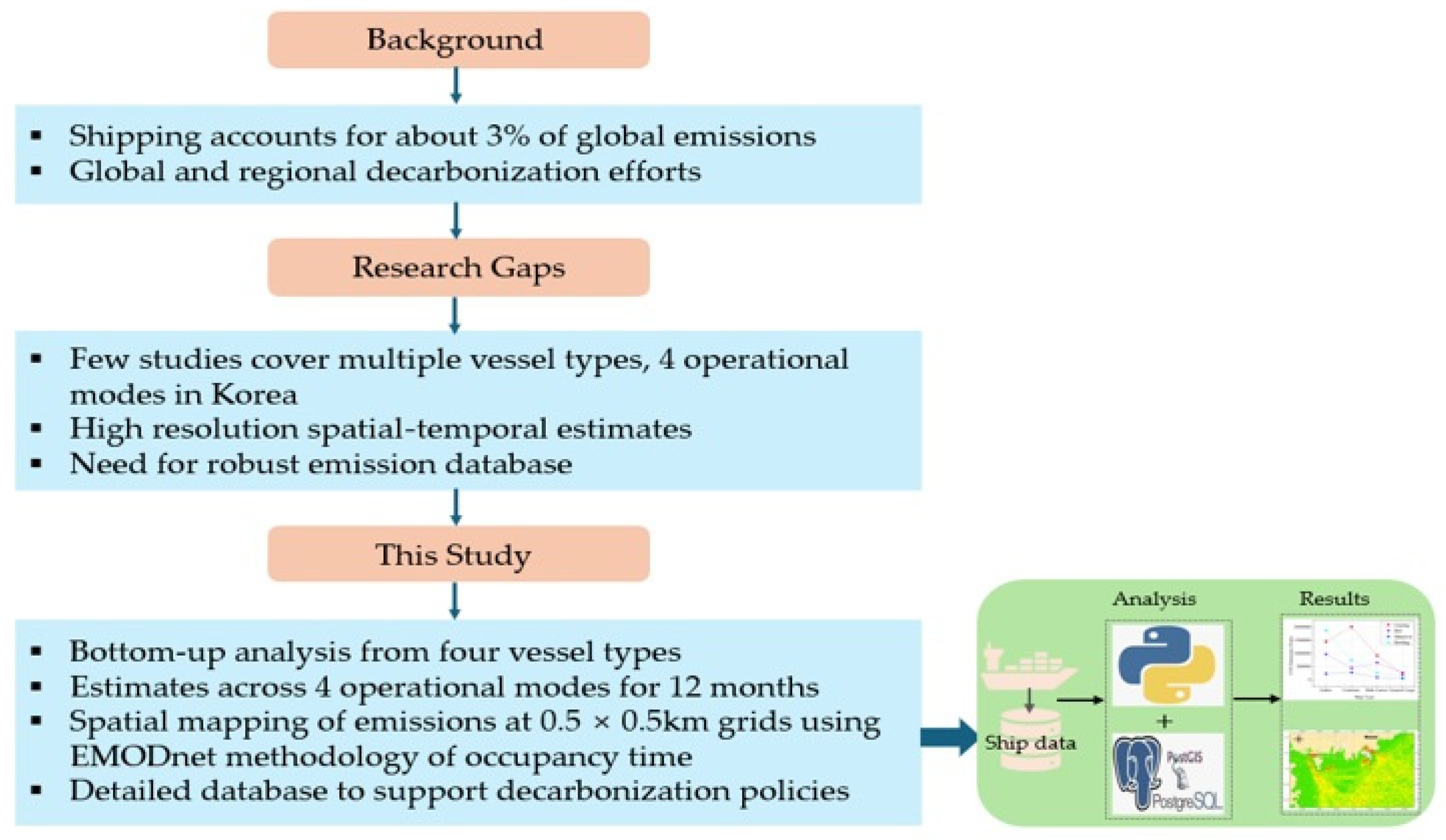
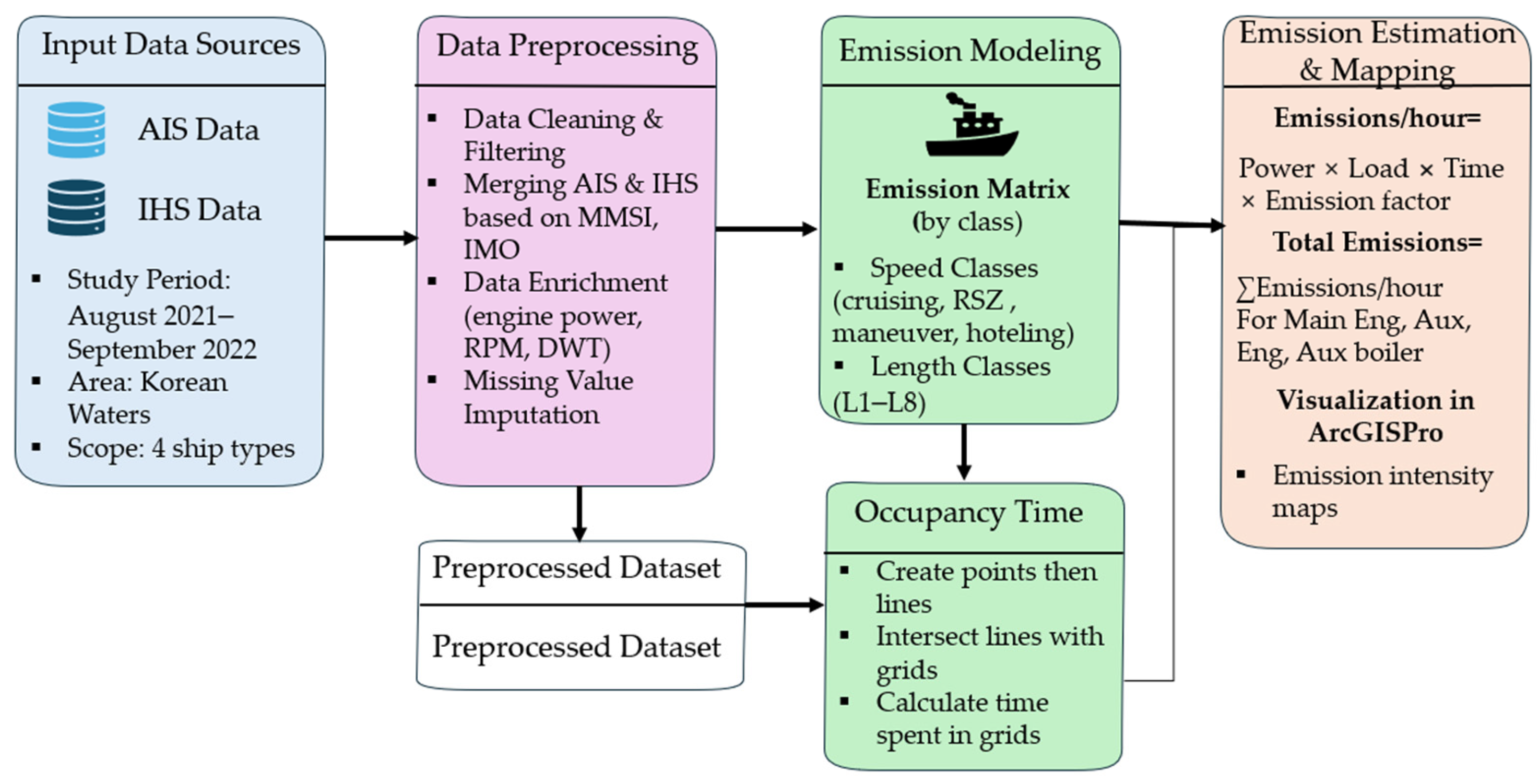
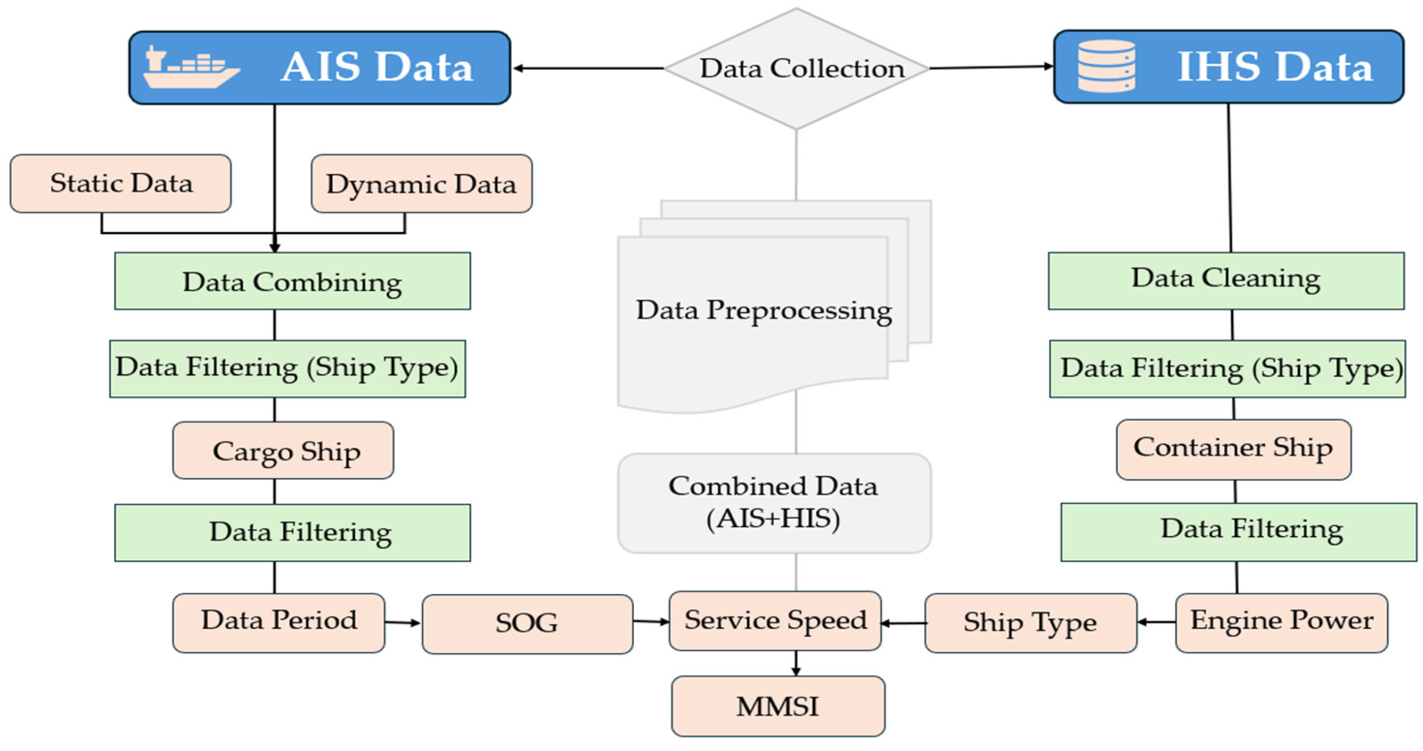
Despite these advancements, few studies have mapped emissions at grid-level resolution using spatial occupancy metrics and aggregated grid spatial emissions. This study responds to the global efforts to reduce maritime emissions and utilizes a comprehensive, data-driven emission estimation framework for vessels operating within the Republic of Korea’s coastal waters. Over a period of 12 months (September 2021–August 2022), exhaust gases of CO2, NOx, and SOx were calculated for four major vessel types: tankers, container ships, bulk carriers, and general cargo vessels across four distinct operational modes, such as cruising, RSZ, maneuvering, and hoteling. This study integrates Automatic Identification System (AIS) data, IHS ship registry data, and spatial grid modeling (0.5 km × 0.5 km) to generate detailed, high-resolution maps of exhaust emissions, all visualized using ArcGIS Pro. What sets this study apart is the application of the spatial-temporal density method, derived from the EMODnet framework, enabling the estimation of vessel occupancy time within grid cells, which is then used to calculate emissions based on the US EPA’s bottom-up modeling formula. Additionally, this research contributes to the creation of a robust maritime emissions database, a resource that is increasingly critical for data-driven decision-making to promote sustainable development. The increasing global efforts to decarbonize shipping, with the IMO targeting net zero by around 2050, presents a pressing need for transparent, traceable, and high-resolution emissions data. Maritime stakeholders, including governments, port authorities, and environmental regulators, require insights into when, where, and why emissions occur, categorized per vessel type, operational mode, engine profile, and pollutant class. By combining operational data, this study provides detailed information, thereby availing opportunities for sustainable management of shipping pollution. 
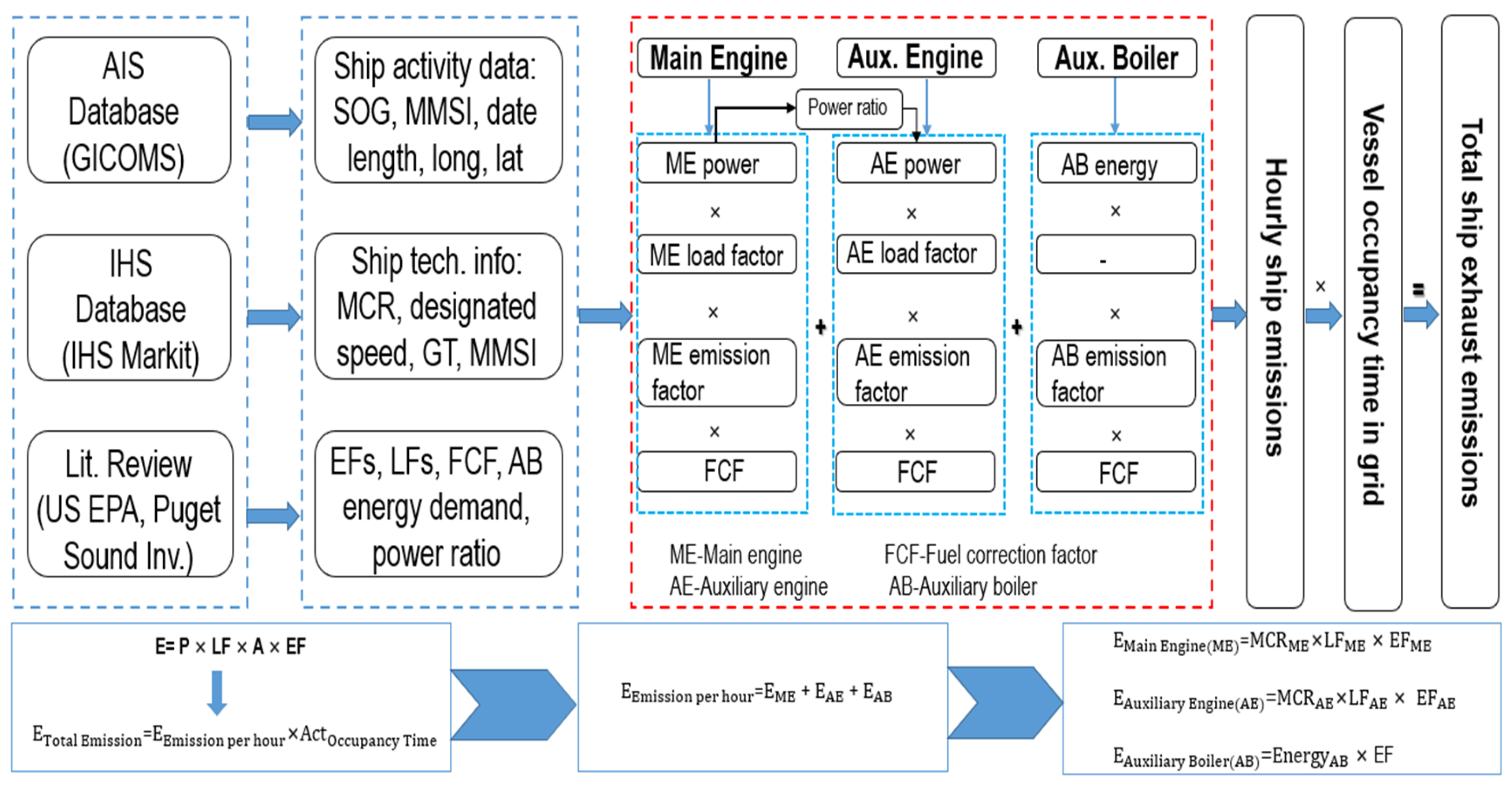
Figure 1 is an illustration of the study background, the research gaps in current research, and how this study aims to enhance the current emission databases.
The remaining sections are divided as follows: In Section 2, details of the data preprocessing steps, emission estimation, and spatial methods are provided. Section 3 presents the emission characterization results for different categories. Section 4 highlights the discussions of the study results. In Section 5, we summarize the study and describe its limitations and future research tasks.

2. Materials and Methods

This study was conducted in the Republic of Korea to analyze the exhaust gas emissions generated by vessels operating in the region. The Republic of Korea’s entire coastal area was designated as the area of interest (AOI) for the study, as shown in Figure 2a. Additionally, grids of 0.5 km by 0.5 km were created over the Republic of Korea’s area, as illustrated in Figure 2b. The grid cell size was chosen to allow for higher spatial resolution when visualizing the emissions in each grid. As shown in Table 1, the AIS data collection period is 12 months, from September 2021 to August 2022. The data volume sums up the values for the tankers, containers, bulk carriers, and general cargo ships at all speeds of navigation.

2.1. Area of Study

Figure 3 is a flowchart of the analysis steps conducted in this study. First, we input the data from various sources, such as AIS and IHS, for the study period and area. The data preprocessing steps entailed data cleaning, filtering, merging, and enrichment to ensure all columns needed for emission calculation are available, and finally, imputation to infill all missing values. Then, the emission modeling process involved the creation of an emission matrix area analysis to define an area of interest and define the grids. The emission matrix was generated based on vessel length and speed to group the emissions by case and then the occupancy time calculation for each grid. Finally, emission analysis entailed calculating the hourly emissions for each equipment and multiplying the hourly emissions by occupancy to obtain total emissions in the grids. Additionally, statistical maps of exhaust gases were done using ArcGIS Pro version 3.0 software, manufactured by ESRI with headquarters in Redlands, CA, USA.

2.2. Data and Characteristics

To prevent collisions at sea, the IMO established a regulation that required vessels to install AIS instruments on all international ships with gross tonnages (GT) of more than 300 GT, on domestic cargo ships with 500 GT and above, and on all passenger ships regardless of size [33]. AIS transmits static data in real time, allowing adjacent ships to recognize other vessels’ statuses and movement. AIS transponders have satellite receivers capable of collecting AIS data over the open sea that are also available [39]. The data contains vessels’ static information, including the ship name, Maritime Mobile Service Identity (MMSI), ship type, length, width, and draught, while the dynamic information provides the navigation status, speed, Course over Ground (COG), Heading over Ground (HOG), and position [40]. Nonetheless, AIS data are limited to ship technical data such as engine power that is required in estimating ship emissions. Therefore, the IHS database from Lloyd’s Register is used to complement the AIS data. The IHS database covers all seagoing merchant vessels of over 100 GT and has valid IMO numbers. The data are continuously updated with newly built ships and provide a range of ship information, including the IMO number, deadweight (DWT), engine power, and revolutions per minute (RPM).

2.3. Data Preprocessing

Data directly taken from the source will likely have inconsistencies and errors and, hence are not ready to be used for a data analysis process [41]. The preprocessing steps of the study data are shown in Figure 4. First, the static and dynamic AIS data are combined and then filtered according to IMO’s defined ship-type numbers to obtain the ship types. However, AIS data only provide generalized cargo data, so to obtain the specific vessel types under cargo data, the AIS database was matched to the IHS database based on IMO or MMSI numbers to distinguish container, bulk carriers, and general cargo ships. For tankers, the AIS data were sufficient to identify the fleet as defined by IMO. The data were filtered according to the ship-type profile, and then the necessary columns required for analysis were obtained. These columns are the date, latitude, longitude, MMSI, LOA, deadweight, service speed, SOG, ship type, and main engine power.
Missing value imputation is a basic solution method for incomplete dataset problems, particularly those where some data samples contain missing attribute values [42]. The study data had a lot of missing parameters, including deadweight, length overall, main engine power, speed over ground (SOG), service speed, and maximum speed. Rows with incomplete values for deadweight were deleted since they were a smaller percentage. Then, applying correlation analysis between parameters (length vs. deadweight and power vs. deadweight), polynomial regression analysis was applied to infill the missing length and power values. Fitted curves of the regression analysis are shown in Figure 5 for all four vessel types.
The analysis generated r-squared values for tankers at 0.71, containers at 0.81, bulk carriers at 0.96, and general cargo at 0.76. While polynomial regression models demonstrated strong fits, especially for bulk carriers (R2 = 0.96) and containers (R2 = 0.81), there remains inherent uncertainty in the imputed values. Factors such as the vessel age, engine retrofits, or hull design may influence the power output in ways not captured by deadweight alone. Therefore, these estimates, though statistically supported, may not perfectly reflect the actual values for all vessel classes, thereby introducing errors in the results. For maximum speed and service speed, the missing parameters were backfilled by considering the characteristics of ships with similar lengths and speeds. Each of the vessel types was divided into emission matrices based on their speed and length, and then the mean values calculated within each class were assigned to the missing data rows.

2.4. Occupancy Time Analysis

Occupancy time refers to the duration a ship spends at a specific location. Occupancy time is critical in estimating maritime pollution, as it describes vessel activity within space. Vessel activity can be determined through the spatial-temporal density technique developed by the European Marine Observation and Data Network (EMODnet) [43]. Before calculating the occupancy time of the vessels under study, ArcGIS Pro software was used to designate the area of analysis and create grids of 0.5 km by 0.5 km over the relevant sea area. Grid cells of 0.5 km by 0.5 km were chosen to enable higher spatial resolution since smaller grid cells allow a more detailed representation of emissions in space. Ships’ hourly emissions vary throughout their voyage depending on the operational mode (speed), type, and size. As a result, the combined preprocessed data are classified using the Python program version 3 as an emission matrix. Python is an open-source language developed by Guido van Rossum and maintained by the Python Software Foundation, whose initial registered office is in Delaware, USA. The grid cells defined in ArcGIS and the emission analysis matrix are input into the Structured Query Language (SQL) database using the PostgreSQL and PostGIS programs version 16. PostgreSQL is derived from a POSTGRES package written at the University of California at Berkeley, whereas PostGIS is developed by Refractions Research Inc. based in Victoria, British Colombia and Canada. The occupancy time of the ships in the grid cells is calculated using the spatial-density analysis method, which applies an SQL syntax. The method considers vessel movement distance with the concept of space and time simultaneously. The spatial-temporal density method creates lines by connecting two consecutive positional points and then calculates the time and distance of the connected line [43]. It also calculates the time within each cell, referred to as the occupancy time for the generated line. The obtained occupancy time is multiplied by the hourly emissions to generate total exhaust gas emissions in each grid cell. Finally, the results are exported as a polygon layer to the ArcGIS program, where the calculated values are constructed as space–time statistical maps. The detailed procedure is demonstrated in Figure 6.
There is a wide range of methods for analyzing the density of vessel passage, including point, line, and vessel density. However, in this study, the occupancy time of the ships in the grid cells is calculated using the spatial-density analysis method. The method considers vessel movement distance with the concept of space and time simultaneously. The spatial-temporal density method creates lines by connecting two consecutive positional points and then calculates the time and distance of the connected line. The procedure also calculates the time within each cell, referred to as the occupancy time for the generating line, as shown in Figure 7 below. Figure 7 is an example of a voyage, whereby the green line’s occupancy time in the cell is determined as 92.5 s by dividing the length covering the grid (370 m) by the entire length (600 m) and then multiplying by the line time given as 150 s. In this study, the occupancy time refers to the duration in which emissions occur within a space range at the time the ship is in the cell. Therefore, the emissions in the grid can be determined by multiplying the occupancy time and the ship’s activity in the cell, which depends on its operational mode and type.

2.5. Emission Output Modeling

Maritim studies commonly apply two approaches for emissions modeling: top-down and bottom-up. In this study, we adopted the bottom-up approach as recommended by the US EPA, which estimates vessel exhaust emissions based on actual ship activity data such as the ship’s speed, engine power, load factor, and activity time. This model for emissions output entails the estimation of quantitative pollutant data from the oceangoing vessels, enabling localized, high-resolution assessments of exhaust gases at the vessel level.
The bottom-up approach for ship emission estimation is widely regarded for its high spatial and temporal resolution, enabling detailed analysis of emissions based on vessel-specific operational characteristics such as engine power, load factors, and activity time [36], unlike the top-down approaches, which rely on aggregate fuel consumption data and are less suited for local-scale analysis. However, despite its advantages, the bottom-up approach is sensitive to the quality and completeness of data input. Missing technical information, such as engine power, or imprecise vessel specifications, such as operational mode, introduce uncertainty through emission calculations. Moreover, assumptions regarding constant load factors or vessel behavior during certain operational modes may not reflect real-world variability [34]. Model outputs are especially affected by inaccuracies in AIS-derived speed data and imputed technical values, which are often estimated through regression models. Furthermore, discrepancies can arise when matching AIS data to fleet registries, particularly in large datasets with older vessels or incomplete identifiers. Hence, although the bottom-up method is robust for localized emission mapping, authors must account for uncertainties tied to data imputation, operational assumptions, and technical variability. The modeling process applied in this study incorporates emission formulas based on engine specifications and operational phases recommended by the US EPA. Further, an emission matrix based on the ship’s speed and length is utilized to obtain emission results based on the operational characteristics of the ships.

2.5.1. Emission Matrix

Ship size is a critical factor in maritime operations and emissions calculations. The most important indicators of vessel size are deadweight, gross tonnage, length overall (LOA), beam, and draft. The ship size index used in this study was selected by considering the Spearman correlation between the size index, navigation speed, and maximum power output. The results revealed a positive correlation between the ship’s overall length, navigation speed, and maximum power output. Therefore, based on these results, vessel length was divided into eight length categories with an incremental length of 50 m. Figure 8 shows graphs of the correlation results.
For navigation speed, the operational mode of the ship was considered, as highlighted in Table 2. While in service, vessels operate in these phases: hoteling, maneuvering, and cruising. According to [7], ships move inside the port boundary with all engines running and at service speed when cruising, while during maneuvering, they transit between the breakwaters with a slower speed maintained as the vessel approaches the pier/wharf/dock. At the reduced speed zone, vessels move at speeds less than cruise but greater than maneuvering. South Korea introduced the VSR program, where ships are mandated to reduce their speeds within certain levels to reduce emissions from OGVs as they enter the ports. In the VSR program in Korea, vessels operate at speeds between 8–10 knots, depending on the vessel type [13]. During hoteling, ships may be at anchorage waiting for a berth call, or they may be at berth with the propulsion engine off, and only the auxiliary engine and boiler operate at peak loads to provide power onboard and for loading and off-loading equipment. In ports where cold ironing is applied, ships use shore power instead of auxiliary engines. In this study, vessels are assumed to operate auxiliary engines during the hoteling mode since the ship data used (2021–2022) were at a period when cold ironing had not been implemented in most Korean ports. The operating phase can determine a ship’s power demand, which is essential when estimating exhaust gases.

2.5.2. Emission Estimation Method and Parameters

The research applies the bottom-up method, based on AIS and IHS data, to estimate exhaust gas from ships. The methodology reflects the ship’s real-time movements and demands the use of detailed specifications data; hence, the results are more accurate [37,44,45]. The three main sources of exhaust gases are the main engine, auxiliary engine, and auxiliary boiler [46]. Ref. [47] mentions that the working conditions of the power equipment vary frequently for different ship movements, leading to significant differences in emissions. When sailing, the ship’s main and auxiliary engines operate at peak loads and generate many waste gases. However, while berthing or mooring, the auxiliary engine and auxiliary boiler are operational; thus, they are the primary sources of pollutants. While some ports worldwide offer shore-side electrical power to allow vessels to switch off their auxiliary engines at berth, this research, which is based in South Korea, assumes auxiliary engines are always on during berthing at South Korean ports. South Korea has initiated the implementation of shore power, also known as Alternative Maritime Power (AMP), at several major ports, but the rollout is ongoing and not yet comprehensive or mandatory for all vessels [48]. Therefore, the use rate of shore power in South Korean ports remains low, and most ships at berth, especially those not equipped or required to use shore power, continue to rely on their auxiliary engines for electricity generation. The Korean government plans to build AMP infrastructure in 230 berths by 2030 in the major ports of Busan, Incheon, Gwangyang, Pyeongtaek-Dangjin, Ulsan, and Pohang [10]. Several pilot projects are ongoing; for example, in January 2025, HMM’s LNG-ready container ship utilized AMP in Gwangyang port in the Republic of Korea, resulting in approximately 16 tons of GHG [49]. With regard to this, the assumption that the vessels at Korean ports utilized auxiliary engines rather than shore is substantiated by the currently existing data and infrastructure. The generalized bottom-up formula for emission determination recommended by US EPA [46] is as in Equation (1):
E = P × L F × A × E F
where E represents the emission of the exhaust gas in grams (g), P is the installed power of the main engine, also called Maximum Continuous Rating (MCR) in kilowatts (kW), LF is the load factor, A is the ship activity time, and EF is the emission factor in grams per kilowatt-hour (g/kWh). Equations (2) and (3) provide the generalized formula, while Equations (4)–(6) are detailed emission formulas for each equipment that emits pollutants as follows:
E T o t a l   E m i s s i o n = E E m i s s i o n   p e r   H o u r × A O c c u p a n c y   T i m e
E E m i s s i o n   p e r   H o u r = E M E + E A E + E A B
E M a i n   E n g i n e ( M E ) = M C R M E × L F M E × E F M E
E A u x i l i a r y   E n g i n e ( A E ) = M C R A E × L F A E × E F A E
E A u x i l i a r y   B o i l e r ( A B ) = E n e r g y   D e m a n d A B × E F A B
Based on Equation (1), the components for emission estimation are engine power, load factor, emission factor, and activity time. Figure 9 is an illustration of the bottom-up approach framework applied in the study for emission estimation.
1. Engine power (MCR)
Ships typically have three engine types: a main engine for propulsion, auxiliary engine for electricity generation, and auxiliary boiler for steam generation. The vessel-operating phase determines the engine power. Data on ship specifications, including main engine power, maximum design speed, vessel type, engine type, gross tonnage, and deadweight, were obtained from the Lloyd Register database (IHS Markit), as described in Section 2.2 in this study. The installed engine power of a ship is essential for emission estimation; however, some values were missing from the IHS database. To estimate the engine power, a correlation between the ship’s length and deadweight was established, and polynomial regression was applied to infill missing data. The main propulsion values were determined by averaging the MCR values of distinct lengths in all the operating modes. Table 3 highlights a positive correlation between length and power in that longer ships demand more engine power to maintain speed. Container ships have higher power requirements compared to other ship types because they operate at higher speeds to meet their fixed schedules. Tankers and bulk carriers have relatively slower speeds and lower main power values because they have flexible schedules that entail longer waiting times at the ports or berth, while general cargo has moderate power requirements.
On the other hand, the auxiliary engine power installed information is not reported on Lloyd’s database. Therefore, an estimation of the auxiliary engine power was done based on the main engine power adopted from the US EPA report [36]. The values are obtained from a survey conducted by the California Air Resources Board (ARB) on oceangoing ships totaling 327 and can be applied to mid-tier inventory development if no auxiliary power data are available [46]. The ratio of the propulsion engine to auxiliary engine provided by the US EPA [46], as shown in Table 4, was used to determine auxiliary engine power.
2. Boiler energy demand
In addition to auxiliary engines, ships also have auxiliary boilers. Boiler energy demand is the amount of energy required to operate boilers on a ship. Boilers are essential for purposes of heating heavy fuel oil, lubricating oil, or for maintaining specific engine parts at required temperatures. Boilers also provide steam for propulsion in steam-powered vessels. In modern vessels, steam is supplied to auxiliary equipment for electricity or freshwater generation and hot water generation for crew needs. During cruising and the reduced speed zone, boilers are typically off because most ships are equipped with exhaust heat recovery systems that utilize heat from the main engine exhaust for hot water needs [46]. When the main engine’s temperature falls below an adequate amount for waste heat recovery, such as during maneuvering and hoteling, the boilers can be operated. For boiler energy demand, the values recommended by the US EPA [46] shown in Table 5 were applied for each vessel type and activity.
3. Load factor
The shipload factor is the percentage of the actual output power to the installed capacity of the ship’s power equipment. It determines how efficiently fuel is burned, affecting the composition of pollutants [50]. Using the Propeller Law, the main engine’s load factor of the ship main engine can be obtained. The calculation formula is in Equation (7):
L F = A S 3 M S
where AS represents the actual speed of the ship obtained from the AIS database, and MS represents the maximum speed of the ship in knots extracted from the IHS database. The load factor of the main engines calculated using the Propeller Law is determined for the four vessel types at different operational modes. On the other hand, the auxiliary load factor is extracted from the research report of the US EPA [46], as illustrated in Table 6. The US EPA provides guidance on assumptions of the load factors as part of their methodology for estimating emissions from marine vessels. The load factor assumptions from the US EPA report vary based on ship type and operation mode.
4. Emission factor
Emission factors vary for engines with different speeds. When the load factor of the main engine is greater than 20%, the emission factor is considered constant, but it increases as the load factor decreases to less than 20%. There is limited data from which emission factors can be obtained, as emission testing of OGVs is relatively difficult and expensive. The emission factors provided in the US EPA report are from an analysis published by Entec highlighting individual factors for slow-speed engines, medium-speed engines, high-speed engines, steam turbines, gas turbines, and the three fuel types (HFO, MDO, and MGO) [46]. The US EPA [46] report has provided emission factors for different pollutants and fuel types for each of the combustion equipment; the values are as indicated in Table 7. In this study, it is assumed that all the vessels used MDO with a 0.5% sulfur content outside ECAs, and a MGO with a 0.1% sulfur content within the ECAs as per IMO regulations.

3. Results

This section highlights the results of emission calculation for the vessel types operating in the Republic of Korea for a period of one year calculated using the methodology mentioned above, with the values rounded off to one decimal point.

3.1. Results of Occupancy Time Analysis

Table 8 is a summary of the total occupancy time in hours for each vessel in each mode. From the results, bulk carriers have the highest total occupancy time. These ships transport bulky raw materials such as coal and grain that may require complex and lengthy loading and unloading times compared to containerized cargo, which are handled using standardized equipment. On the other hand, tankers have the highest occupancy time in the Reduced Speed Mode (RSZ) compared to other ship types because of operational and regulatory factors. Tankers transport large quantities of oil and gas, making them subject to stricter environmental regulations. Tankers may need to travel at much slower speeds for longer periods when entering certain regions to minimize the risk of accidents such as oil spills. In the cruising phase, containers had the highest occupancy time of all other ship types because of their operational patterns that resulted in frequent movements. Overall, container, bulk carriers, and general cargo had the highest occupancy time in the hoteling phase compared to other operation modes due to potentially longer waiting times at the ports. However, tankers had the lowest occupancy during hoteling because they dock at specialized terminals designed to handle specific liquid bulk cargo, making it less likely for them to wait for longer hours for an available berth.

3.2. Ship Emissions per Each Equipment

The main engine emits the largest pollutants for all vessels and pollutant types because the main engine operates at higher loads. However, it is worth noting that for tankers, emissions from the main engine and the auxiliary boilers are almost at the same level, while the emission levels from these two pieces of equipment were significantly different for the other ship types. Table 9, Table 10 and Table 11 present the results of emissions for the three equipment, rounded off to one decimal point. For the CO2 emissions in Table 9, tankers had the highest total emissions (4,543,196 tons), with significant contributions from auxiliary boilers; for the NOx emissions in Table 10, tankers and container vessels emitted similar levels of approximately 64,000 tons each, dominated by main engine exhaust. Table 11 of the SOx emissions results highlights tankers again as the highest contributors, with about 13,937.7 tons, followed by container vessels and bulk carriers.
Figure 10 presents the main engine emission inventory. Tankers and containers had the highest emissions, with tankers slightly leading because they have larger engines with higher fuel requirements. Container ships also consume large amounts of fuel due to their need to maintain high speeds and operation frequency. Bulk carriers have moderate emissions, while general cargo ships have the lowest due to their small size and lower fuel consumption.
For the auxiliary engine shown in Figure 11, the results are different from the main engine inventory. Here, container ships emit slightly higher CO2, NOx, and SOx exhaust gases compared to tankers. Auxiliary engines on container ships have higher operational demands during port stays, which explains the high emissions. Bulk carriers and general cargo had lower emissions, which is consistent with their lower auxiliary engine usage compared to tankers and containers.
The auxiliary boiler emission inventory in Figure 12 revealed the highest CO2, NOx, and SOx emissions from tanker vessels with significant differences compared to other ships. Auxiliary boilers on tankers are frequently used for cargo operations, such as heating oil for viscosity control and other processes that demand significant fuel consumption. Containers, bulk carriers, and general cargo have minimal emissions, reflecting that they are less reliant on boilers. Only CO2 and SOx emissions are significantly high from tankers, but NOx pollutants are very low. The disparity occurred because CO2 emissions directly correlate with the amount of fuel consumed during operation. Similarly, SOx exhaust gases directly relate to sulfur fuel, and tankers use high-sulfur fuels. However, NOx formation is more dependent on combustion temperatures rather than fuel amount or sulfur content.

3.3. Ship Emissions by Vessel Type

The summarized emissions per ship type are presented in Table 12, with the values rounded off to one decimal point. Tankers recorded the largest emissions, accounting for approximately 4,601,007.1 tons, followed by containers at 3,546,082.8 tons. General cargo had the least amount of emissions, totaling around 676,690.3 tons, because of their small number in operation and the use of small engines that consume less fuel compared to the other ship types.

3.4. Ship Emissions by Operation Mode

Table 13, Table 14 and Table 15 present detailed results for emissions categorized by the operational mode. Container ships generated peak emissions during cruising and maneuvering. However, overall, the tankers had the highest total emissions combined in all phases due to significantly large pollutants released during the hoteling mode. Although tanker ships had shorter activity times during hoteling, they were the largest emitters of CO2, illustrated in Table 13, because of high energy demands when stationery for oil heating, operation of cargo pumps, and other safety equipment for handling its cargo during loading or unloading operations. Crude oil carriers demand a continuous supply of heat to maintain an optimal temperature for the oil. Additionally, tankers still use less efficient fuels while in ports; therefore, although they spend less time in ports or at berth, their emissions are disproportionately higher than other vessels that use systems that are more efficient and cleaner fuels.
Bulk carriers and general cargo vessels showed moderate but non-negligible emissions across all modes. General cargo ships produced the lowest emissions in all modes due to their smaller size and shorter cruising time. Tankers and containers have the highest NOx emissions, particularly when cruising when their engines operate at higher loads and higher temperatures. Bulk carriers showed notable NOx pollutants when operating in the RSZ, as shown in Table 14. All the vessels had the lowest NOx emission during maneuvering since engines typically operate at lower loads during port entry or exit. Containers emitted the highest SOx emissions in the cruising mode, while tankers were the largest contributors of SOx during hoteling, as indicated in Table 15. This can likely be explained by the large fuel consumption by containers and tankers when sailing. During hoteling, tankers use heavy fuel oil, which has a higher sulfur content than marine diesel oil or marine gas oil utilized by other ship types, leading to high SOx emissions.

3.5. Ship Emissions by Pollutant

Table 16 consolidates the exhaust gases by pollutant (CO2, NOx, and SOx) across all vessel types. CO2 dominated the total emissions, accounting for a higher majority of total tonnage. The total CO2 emissions from tankers, containers, bulk carriers, and general cargo vessels were approximately 10,478,392.7 tons. Tankers accounted for about 43.3%, containers 33.1%, bulk carriers 17.3%, and general cargo 6.3%. For NOx, tankers emitted 33.6%, containers 34%, bulk carriers 26.2%, and general cargo 6.3%. On the other hand, SOx emissions were 42.9% for tankers, 32.8% for containers, 18.1% for bulk carriers, and 6.3%, as highlighted in Table 16. Similarly, Figure 13 is a visualization of the variations in emissions across operational modes and vessel types for CO2, NOx, and SOx. Distinct peaks are observed for container ships during cruising, while tanker emissions peak sharply during hoteling operations.

3.6. Emission Distribution

This section provides the spatial visualization of the total emissions over a period of 1 month (1–31 January 2022) in a major port in South Korea from the four ship types using a Geographic Information System. After estimating the vessel density for each grid cell through spatio-temporal analysis in PostgreSQL/PostGIS, the data were combined with vessel-specific hourly emission values that were calculated for the four ship types and four operational modes to estimate the total emissions. The emissions output was then imported into ArcGIS Pro using PostGIS to generate detailed emission intensity maps using a 0.5 km by 0.5 km grid system. The spatial maps illustrate the emissions distribution with significant spatial differences based on the ship-type operation in the region. These maps provide a visualization of where the emissions are most concentrated, providing a basis for environmental monitoring and the establishment of pollution control policies.
The emission distribution maps in Figure 14, Figure 15 and Figure 16 highlight distinct spatial differences across vessel types. Overall, container vessels exhibit high emission densities in the approach channels and anchorage zones near Busan Port, corresponding to their frequent maneuvering and prolonged hoteling. Tankers show more dispersed emissions patterns, reflecting their activity across outer harbor zones and anchoring areas. In contrast, general cargo ships show moderate and more spatially uniform emission footprints, particularly along secondary routes, while bulk carrier emissions are minimal. The visualized emission patterns directly correlate with the operational behavior and port usage characteristics of each vessel type. Detailed discussions of the spatial distribution maps for all the pollutant types are done below.
Based on the emission maps in Figure 14a, emission clusters are observed in Busan North Port and its anchorage area near Yeongdo–gu. Busan North Port is a major hub for various maritime operations, including handling oil and chemical products. The emissions result from the use of boilers during cargo operations as tankers use this zone. The west of the North Port also has an emission cluster, as it could be an outer anchorage area used by tankers awaiting berth assignments or clearance to enter regulated port waters. In contrast, container vessel CO2 emissions show the highest concentrations symbolized by red clusters in the North Port and New Port and in their anchorage areas, as shown in Figure 14b. Busan is the largest container handling port in South Korea, processing millions of twenty-foot Equivalent Units (TEUs) annually. There are concentrated emissions near the container terminals in the North Port, New Port, and anchorage areas. The dense red clusters highlight intense port and anchorage activities with emissions being generated during maneuvering and hoteling modes. Bulk carrier CO2 emissions are significantly less in Busan and primarily located in anchorage zones due to their longer hoteling times during loading and unloading of cargo. For general cargo in Figure 14d, noticeable emissions are seen on the vessel tracks approaching/leaving the North Port anchorage area. General cargo vessels transport a wide variety of cargo, typically in smaller quantities, and their emissions are dispersed, aligning with operational routes.
For tankers, low quantities of NOx exhaust, likely resulting from maneuvering and low-speed operations near anchorage zones, can be observed around the North Port, as shown in Figure 15a. NOx emissions from container ships, in Figure 15b, show the most significant concentrations in Busan, especially in the North Port and New Port. Medium–intensity emission tracks can be seen in the navigation channels approaching Busan ports. The constant flow of large container ship traffic in Busan leads to high NOx exhaust during port entry and exit. The clustered patterns of medium intensity near the terminals indicate high activity during maneuvering. Container vessels operate at higher engine loads during cruising and maneuvering modes, resulting in high temperatures that cause substantial NOx formation. Figure 15c above is the spatial result of the emissions from bulk carriers in the Republic of Korea. The emissions are modest and more spatially dispersed, primarily occurring in anchorage zones rather than on transit paths. On the other hand, distinct NOx clusters along the navigation routes approaching the Busan Old Port anchorage can be observed for general cargo ships, as illustrated in Figure 15d. These emissions result from continuous low-speed movements during the approach or departure of ships.
Tanker ships emitted the greatest SOx emissions compared to other vessel types. SOx pollutants are emitted when sulfur-based fuel is burnt. Therefore, SOx emissions directly correlate to the sulfur levels in the fuel and partly to the quantity of fuel. Figure 16a shows high-intensity emission clusters in the port areas and anchorage areas despite the fuel sulfur limits imposed by the IMO on ships when entering or exiting the ports. Low-intensity emission tracks can also be observed on the fairways, indicating cruise-related exhausts. Despite the high container traffic, SOx emissions are the lowest compared to other vessel types, as seen in Figure 16b. This could be due to the strict enforcement of the 0.1% sulfur fuel limit or the use of scrubbers applied to ECAs. Additionally, large container vessels likely have efficient systems installed that lead to reduced pollution. Clusters of medium-intensity emissions are only visible in the Busan Old Port anchorage, and this could be due to ships waiting in the anchorage zones. Bulk carriers also had lower SOx emissions, as shown in Figure 16c, consistent with their slower operations and less frequent port calls at Busan Port. General cargo also emitted notable SOx exhaust with several high-intensity clusters illustrated in Figure 16d. This could be due to general cargo vessels being older fleets that use less efficient engines or longer waiting times during hoteling and maneuvering. The yellow color signifies medium-intensity pollutants emitted from ships cruising slowly when approaching or departing the port.

4. Discussion

This study aligns with the global and national efforts to reduce maritime pollution by providing a data-driven emission inventory and a detailed analysis of current emissions levels using a bottom-up and spatio-temporal approach. Through the integration of AIS, IHS, and GIS technologies, vessel emissions across different ship types, operational modes, and equipment categories were quantified and mapped for Korean coastal waters, identifying key areas where compliance with international regulations can further minimize the environmental footprint of maritime activities.
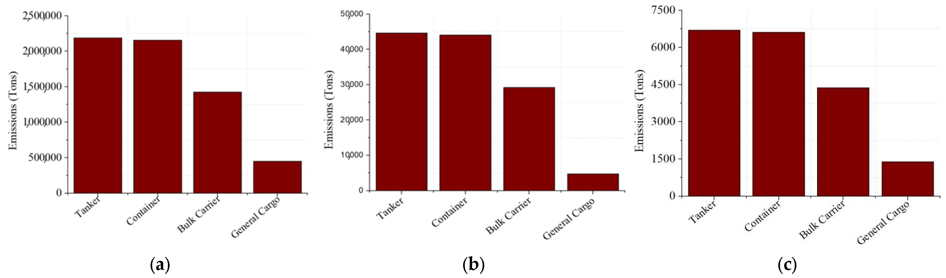
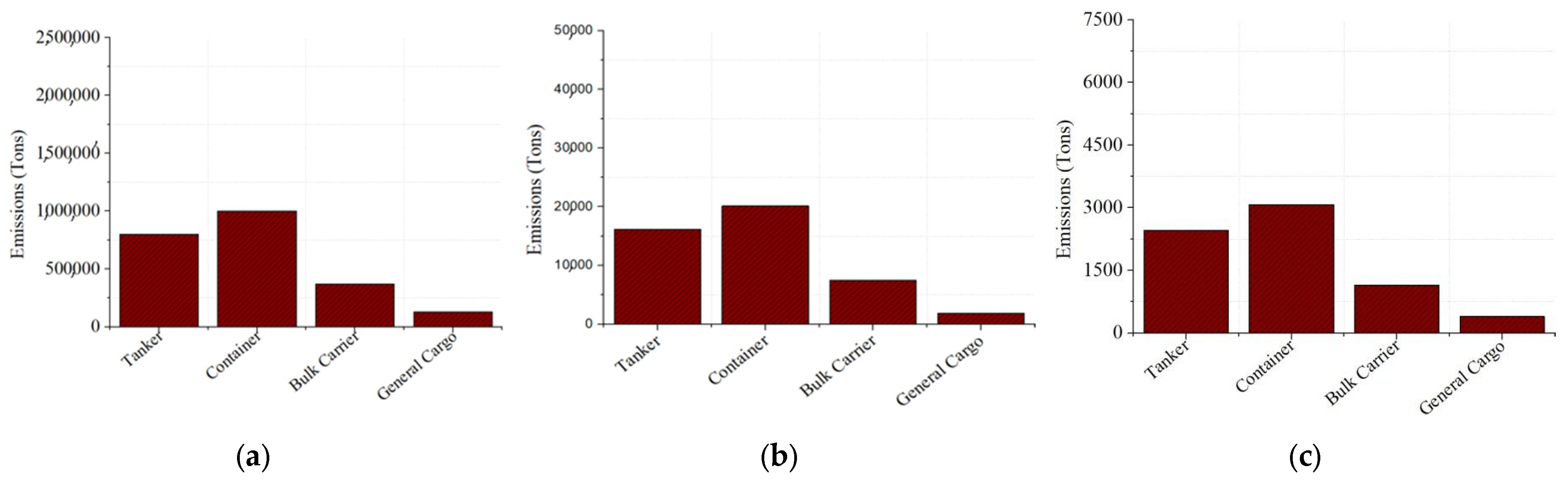
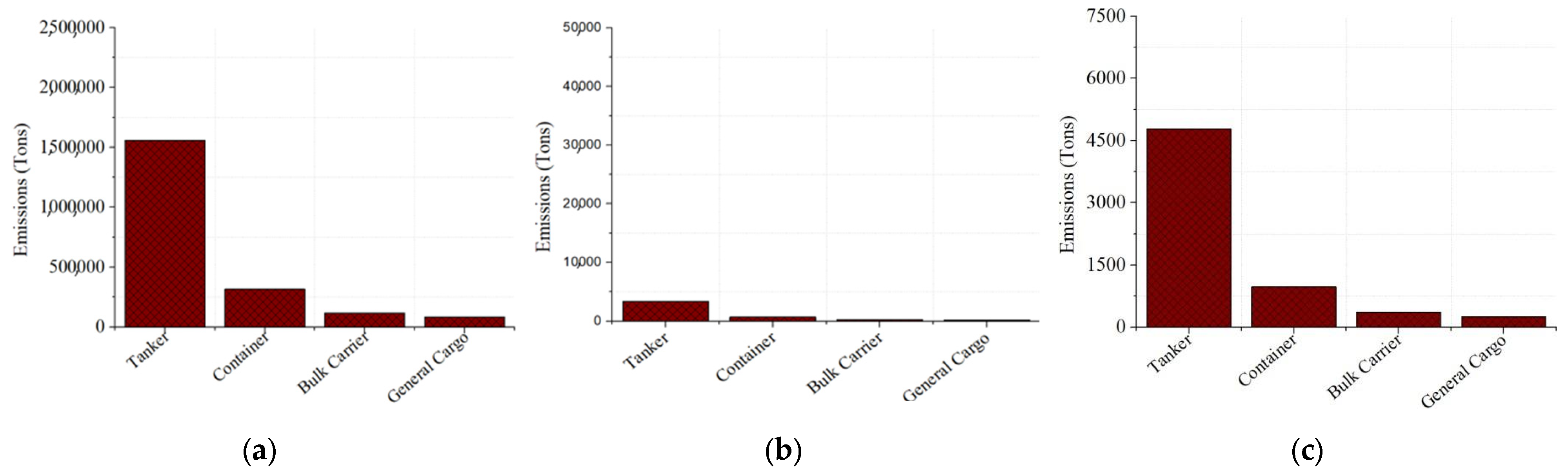
This research revealed significant differences in emissions levels from the four vessel types. Tankers were the largest emitters of CO2, NOx, and SOx emissions, followed by container vessels, bulk carriers, and general cargo ships. As shown in Table 12, tankers accounted for the largest share of CO2, nearly 43.3%, contributing around 4.5 million tons annually, corresponding to [51]’s research that found tanker ships as the highest emitters at Incheon port. Container ships contributed slightly lower CO2 amounts, totaling 3.5 million tons, but emitted comparable levels of NOx, while general cargo had the least value at 6.3%. The dominance of tanker emissions can be attributed to their larger engine sizes, leading to higher fuel consumption, extended hoteling periods, and intensive auxiliary boiler operations during cargo loading and unloading operations. Additionally, there are many tanker ships, accounting for a significant percent of the global fleet; hence, generally, CO2, NOx, and SOx emissions were highest for tanker ships and lowest for general cargo. Table 9, Table 10 and Table 11 showing equipment-specific results emphasize the primary sources of emissions for CO2 and NOx as the main engines, while auxiliary boilers significantly contributed to SO
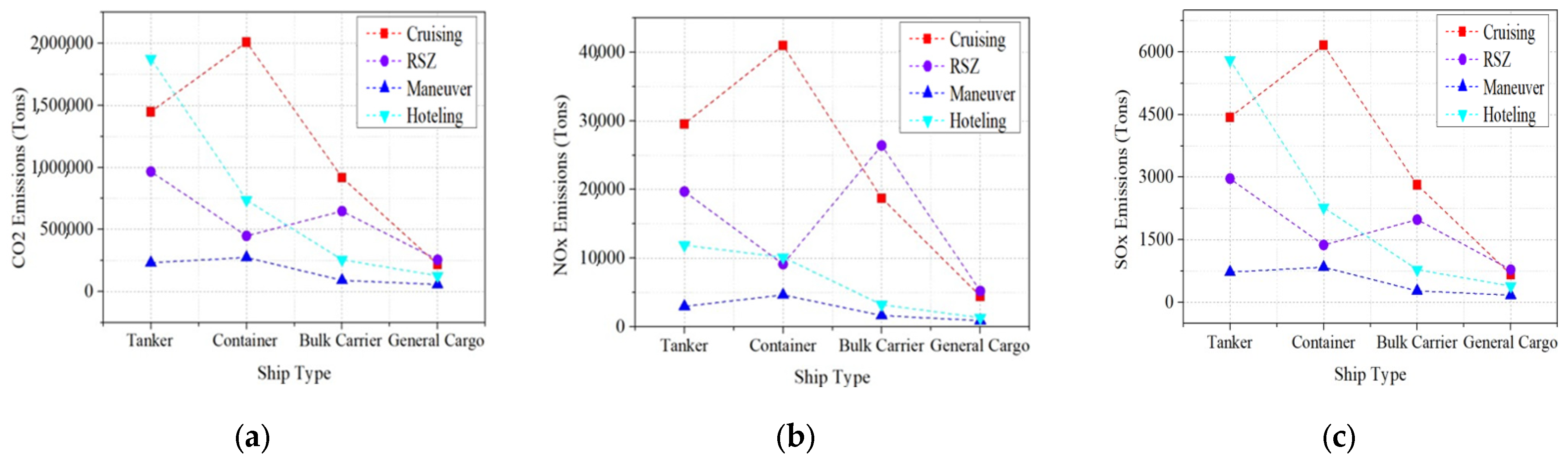
x emissions, particularly for tankers and general cargo ships. The operational mode results presented in Table 13, Table 14 and Table 15 show that the cruising mode generated the highest emissions for container vessels, particularly for CO2 and NOx, compared to other ship types. In contrast, hoteling was a major emission contributor for tankers and bulk carriers due to long idle times at anchorage using auxiliary engines and boilers. This emphasizes the need to expedite the adoption of shore power at major ports like Busan. In the line graphs in Figure 13, emissions during maneuvering and RSZ operations were non-negligible and varied significantly between vessel types, indicating the operational profiles’ critical impact on total emissions.
Overall, this study highlights tankers and containers as major contributors to maritime emissions. Tankers were the largest contributors to the total emissions in Korean coastal waters. Container ships, while contributing slightly lower overall CO2 emissions, exhibited high NOx emissions, particularly during the maneuvering and cruising phases, reflecting their frequent port entries and high-load engine operations. Bulk carriers and general cargo vessels produced lower emission volumes but showed characteristic patterns linked to extended hoteling periods and slow-speed operations near port approaches. These vessel categories, often older and operating less efficiently, contributed a disproportionately higher amount of SOx relative to their CO2 emissions, suggesting the potential use of higher-sulfur fuels. Additionally, vessels generated varying exhaust gases depending on their sizes and operational modes, suggesting that distinct operational characteristics of ships played a critical role in emission levels. The high amounts of CO2 emissions across all ship types suggest that the use of high-quality fossil fuels has been insufficient in minimizing GHG emissions. Therefore, all ship types should be strictly required to adhere to IMO’s energy efficiency standards. Additionally, emphasis should be directed towards the adoption of clean energy sources such as green ammonia or hybrid propulsion options.
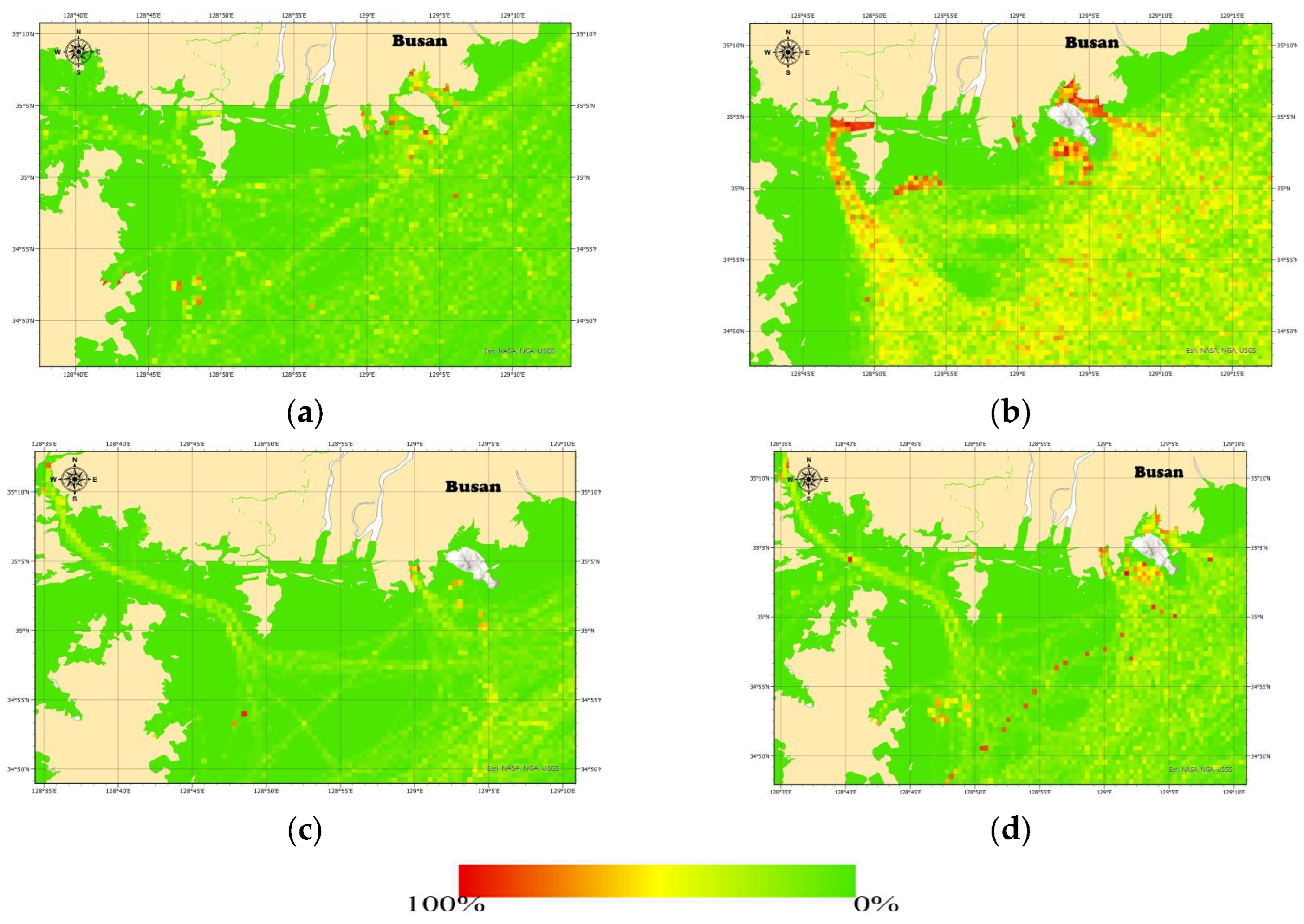
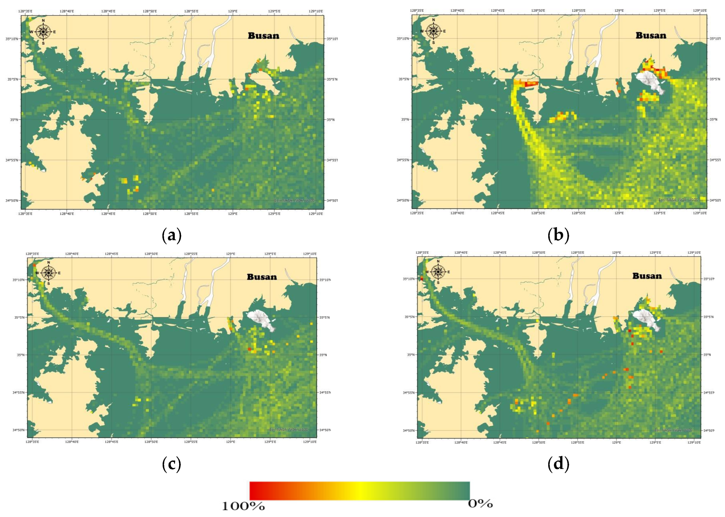
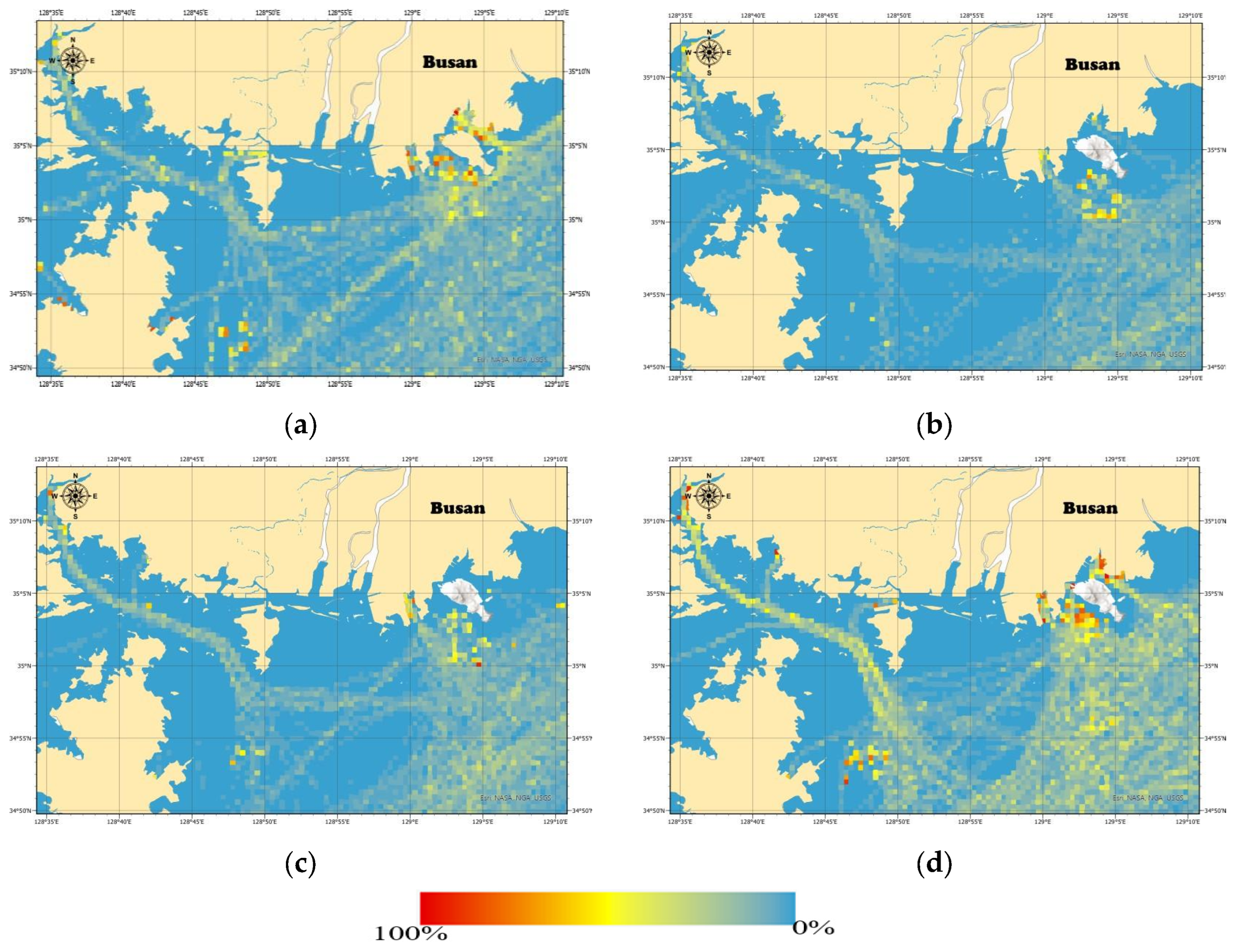
Moreover, this study revealed significant spatial variations in emissions in Busan, highlighting the influence of vessel types and operational modes on emission volumes. The emission hotspots identified through GIS mapping correspond to anchorage zones and the major shipping lanes. Anchorage zones and ship terminals and berths had high-intensity emissions, especially for CO2. In the study, Busan had the highest CO2 emissions clustering from container vessels near the North Port and the New Port, aligning with its position as among the busiest container terminals in the world. However, SOx emissions were notably lower in Busan, primarily concentrated around anchorage zones due to stringent fuel regulations in ECAs. These results highlight the concentration of container shipping activities in Busan Port and the need for localized maritime pollution control strategies. Additionally, the research revealed the need to apply different emission control measures for different vessel types, regions, and shipping activities. For example, tanker and general cargo vessels’ emissions can be significantly reduced by adopting shore power in port areas that experience the highest vessel activities. Promoting the use of shore power in these zones will reduce the environmental impact of stationary vessels at the port. Port authorities should expand the shore power networks and charging infrastructure to allow ships to switch off the auxiliary engines while at ports. Furthermore, improving communication and cooperation between ports will contribute to environmentally friendly port management. On the other hand, container vessels’ cruising emissions can be controlled by finding a balance between speed reduction and maintaining their schedules.
Generally, CO2 emissions were the highest, totaling approximately 10.5 million tons for a period of 1 year. In 2019, Korea’s annual shipping GHG emissions accounted for around 27.4 million tons of CO2-equivalent, representing approximately 3.9% of the total GHG emissions in Korea (about 701.3 million tons of CO2-equivalent) [10]. Additionally, according to the Greenhouse Gas Inventory and Research Center of Korea (GIR), the Republic of Korea’s total GHG emissions in 2022 was reported as 642.8 million tons of CO2-equivalent [52]. Focusing specifically on CO2 from fuel combustion, the total emissions was around 549.31 million tons in 2022 [53]. To contextualize the results of this study, the 10.5 million tons of CO2 emissions estimated from the four vessel types represent approximately 1.9% of the Republic of Korea’s total CO2 emissions from the fuel combustion generated in 2022. The value only represents a percentage of emissions from the shipping sector since this study only covers the four dominant contributors of ship exhaust gases (tankers, containers, bulk carriers, and general cargo). Although this proportion seems modest, it is significant in Korea’s national emissions reduction target since the maritime industry is integral to the region’s development. The prolonged reliance on fossil fuels is a huge hindrance to decarbonization in the Republic of Korea, with research indicating that by 2021, the transport sector will be mostly dominated by fossil fuels [54]. In this study, all the ships used fossil fuels, specifically MDO outside ECAs and MGO within the ECAs. The share of low-carbon fuels in the transport mix needs to increase to between 40–60% by 2040 if the Republic of Korea wants to largely reduce national GHG emissions [55]. Consequently, MOF released the 2050 Net-Zero Roadmap, which sets target emission reductions for Nationally Determined Contributions (NDCs), which include domestic shipping emissions at 40% by 2030 and 70% by 2050 compared to 2018 levels, whereas, for international shipping, the goal aligns with IMO’s 50% GHG reduction in emissions. Furthermore, the Republic of Korea implemented several policies to facilitate emission reductions in its shipping industry. These include a green fleet transition that entails conversion to eco-friendly ships, the use of alternative fuels, the establishment of zero-emission shipping routes, and international corporations [10]. With increasing global pressure to decarbonize and the Republic of Korea’s vision to be among the leaders in shipping and shipbuilding to realize net-zero emissions by 2050, a comprehensive database of current emission levels from Korean ships is paramount. This study complements the existing emission inventories and avails emission data that are vital in promoting the development of targeted emission reduction strategies to achieve the Republic of Korea’s broader climate goal and maintain its competitiveness in global shipping.
The bottom-up methodology combined with the spatio-temporal technique applied in this study generated detailed emission values by vessel type, operational mode, and equipment type, thus contributing to existing emission databases to help mitigate maritime pollution [55]. However, the bottom-up approach still generates uncertainties in the results due to the imputation of missing technical data, load factors, vessel operational behaviors, and lack of integration of dynamic environmental conditions that greatly affect fuel consumption and emissions [32]. Future work should address these uncertainties by incorporating probabilistic modeling, real-time metocean data, and machine learning techniques to refine predictive capabilities. Further, the differentiated emissions by vessel type, operational mode, pollutant type, and spatial location offer actionable insights for maritime stakeholders, including port authorities, regulators, and policymakers. From the findings, port authorities are mandated to expand shore power systems at terminals where hoteling emissions are dominant. Korea has already implemented vessel speed programs at its major ports; however more should be done to further mitigate pollution in its port areas. The government should also increase incentivization for fuel switching or provide retrofit investments based on ship emission profiles as part of its maritime pollution policies. In addition, emission monitoring systems integrating AIS, remote sensing, and onboard reporting should be mandated for all ships to enable South Korea to pursue its carbon neutrality targets along with IMO’s net-zero targets.
To conclude, this study underlines the use of a bottom-up and spatio-temporal analysis approach as a basis for conducting ship-type and mode-specific emission inventories. This has implications for tracking emission changes and understanding its patterns at various levels, which is fundamental for targeted emission reduction strategies that will contribute towards addressing the adverse impacts of ship pollutants in the Republic of Korea’s coastal regions. These findings provide actionable insights for developing differentiated policies aimed at specific vessel categories and operational behaviors, supporting the Republic of Korea’s broader maritime decarbonization goals aligned with the IMO’s net-zero strategy.

5. Conclusions

Shipping is a pivotal industry for global trade and is particularly significant for countries like South Korea that heavily rely on exports. Data-driven decisions play a vital role in the formulation of effective policies with the growing demand for sustainability and IMO’s tightened regulatory frameworks to achieve net-zero emissions in the shipping sector. This study on emissions from ships operating in Korean waters offers a comprehensive analysis of vessel exhaust gases and highlights findings regarding the distribution and intensity of CO2, NOx, and SOx emissions by vessel types, operational modes, and pollutants. The main conclusions are summarized below:
  • Tankers were identified as the largest contributors to CO2 (about 4.5 million tons), NOx (around 64,000 tons), and SOx (approximately 13,900 tons) emissions, followed by container vessels, bulk carriers, and general cargo ships. Further, analysis of operational mode pollution showed that container ships generated the most emissions during cruising, while tankers’ emissions were highest during hoteling.
  • Main engines were the dominant source of CO2 and NOx emissions, whereas auxiliary boilers were significant emitters of SOx emissions, particularly during hoteling for tanker ships.
  • The spatial distribution maps highlighted emission hotspots from container vessels at Busan’s North Port and New Port, emphasizing the influence of vessel density and operational behaviors on pollution patterns.
  • CO2 emissions were the highest, accounting for approximately 1.9% of the total CO2 emissions from fuel combustion in Korea. Therefore, maritime emissions in Korea represent a substantial share of the national CO2 emissions, highlighting an urgent need for more sector-specific mitigation measures.
  • Furthermore, this study validates the significance of spatio-temporal analysis combined with a bottom-up approach for vessel-specific inventories to implement effective decarbonization policies.
This study leveraged maritime big data combined with emission models to enable the accurate spatial mapping of shipping emissions, with the aim of supporting global efforts for minimizing maritime pollution. Thus, it contributed to the existing emission databases that highlight emission characteristics to help formulate effective pollution control policies. This research had implications for tracking emission changes and understanding its patterns according to the mentioned criteria; this is fundamental for targeted emission reduction strategies that will contribute towards addressing the adverse impacts of ship pollutants in the Republic of Korea’s coastal regions. Policy recommendations based on this study include:
  • Expediting the expansion of shore power (AMP) infrastructure at key port terminals in Korea to curb hoteling emissions.
  • Implementing other vessel speed reduction programs at key cruising shipping lanes.
  • Intensifying incentivization programs to promote the operation of low-emission vessels.
In conclusion, this study contributes to the existing research on developing detailed emission databases that provide a foundation for emission reduction strategies contributing to the broader goal of achieving net-zero emissions in shipping. Nevertheless, this study was not sufficient due to the following limitations:
  • First, ships are greatly affected by weather and environmental factors such as wind and waves when sailing that affect fuel consumption and the dispersion of pollutants [50]. In the future, dynamic weather and environmental data should be integrated to make the research more comprehensive.
  • Second, future research should integrate GIS tools with machine learning techniques for dynamic visualizations to help uncover complex trends in emission distributions.
  • Third, although regression-based imputation allowed recovery of missing technical parameters, these models introduced error uncertainties in the overall results. Future work could incorporate probabilistic approaches to better capture this uncertainty or conduct a scenario analysis to assess the influence of imputation on emission results.
  • Lastly, future work should consider the use of satellite emission tracking alongside AIS data to correlate emissions with specific vessels. These improvements will increase the viability of these emission results by enhancing transparency and traceability.

Author Contributions

Conceptualization, I.-S.C., W.-J.S., D.-J.J. and A.W.K.; methodology, D.-J.J.; software, A.W.K. and W.-J.S.; validation, I.-S.C., W.-J.S. and A.W.K.; formal analysis, A.W.K.; investigation, A.W.K.; resources, A.W.K.; data curation, A.W.K.; writing—original draft preparation, A.W.K.; writing—review and editing, I.-S.C., W.-J.S. and A.W.K.; visualization, A.W.K.; supervision, I.-S.C.; project administration, I.-S.C.; funding acquisition, W.-J.S. All authors have read and agreed to the published version of the manuscript.

Funding

This research was funded by the National Research Foundation of Korea (NRF) grant funded by the Korean government (Ministry of Science and ICT (MSIT)), grant number RS-2025-00554193.

Data Availability Statement

This study was conducted using data provided by the Ministry of Oceans and Fisheries (MOF, Republic of Korea) for ship traffic route research.

Conflicts of Interest

The authors declare no conflicts of interest.

Abbreviations

The following abbreviations are used in this manuscript:
GHGGreenhouse gas gases
CO2Carbon dioxides
NOxNitrogen oxides
SOxSulfur oxides
GISGeographic Information System
RSZReduced Speed Zone
IMOInternational Maritime Organization
MARPOLInternational Convention on Maritime Pollution
IPCCInternational Panel on Climate Change
MOFMinistry of Ocean Fishery
AISAutomatic Information System
GTGross tonnage
SEIMShip Emission Inventory Model
ECAEmission Control Area
IHSInformation Handling System
EMODnetEuropean Marine Observation and Data Network
AOIArea of interest
USEPAUnited States Environmental Protection Authority
GBGigabyte
MMSIMaritime Mobile Service Identity
HOGHeading Over Ground
COGCourse Over Ground
DWTDeadweight
RPMRevolutions Per Minute
SOGSpeed Over Ground
SQLStructured Query Language
LOALength overall
VSRVessel speed reduction
OGVOcean Going Vessels
AMPAlternative Maritime Power
HMMHyundai Merchant Marine
LNGLiquefied natural gas
MCRMaximum Continuous Rate
LFLoad factor
EFEmission factor
MEMain engine
AEAuxiliary engine
ABAuxiliary boiler
FCFFuel Correction Factor
ARBAir Resources Board
HFOHeavy fuel il
MDOMarine diesel oil
MGOMarine gas oil
TEUTwenty-foot Equivalent Units
GEEMGeographic Emission Estimation Model
KMIKorea Maritime Institute
GIRGreenhouse Gas Inventory and Research
NDCsNationally Determined Contributions

References

  1. Kwon, Y.; Lim, H.; Lim, Y.; Lee, H. Implication of activity-based vessel emission to improve regional air inventory in a port area. Atmos. Environ. 2019, 203, 262–270. [Google Scholar] [CrossRef]
  2. United Nations Conference on Trade and Development (UNCTAD). The UNCTAD Handbook of Statistics 2021; UNCTAD: New York, NY, USA, 2021. [Google Scholar]
  3. IMO. Second International Maritime Organization GHG Study 2009: Update of the 2000 IMO GHG Study; IMO: London, UK, 2009. [Google Scholar]
  4. Bilgili, L.; Celebi, U.B. Emission routing in maritime transportation. In Energy, Transportation and Global Warming; Springer: Berlin/Heidelberg, Germany, 2016; pp. 837–849. [Google Scholar]
  5. Carlton, J.S.; Danton, S.D.; Gawen, R.W. Marine Exhaust Emissions Research Programme; Lloyd’s Register Engineering Services: London, UK, 1995. [Google Scholar]
  6. Eyring, V.; Köhler, H.W.; Lauer, A.; Lemper, B. Emissions from international shipping: 2. Impact of future technologies on scenarios until 2050. J. Geophys. Res. Atmos. 2005, 110, 1–23. [Google Scholar] [CrossRef]
  7. Song, S. Ship emissions inventory, social cost and eco-efficiency in Shanghai Yangshan port. Atmos. Environ. 2014, 82, 288–297. [Google Scholar] [CrossRef]
  8. Merk, O. Shipping Emissions in Ports; International Transport Forum: Paris, France, 2014. [Google Scholar]
  9. IMO. Fourth IMO Greenhouse Gas Study 2020: Safe, Secure and Efficient Shipping on Clean Oceans; International Maritime Organization (IMO): London, UK, 2021. [Google Scholar]
  10. Yum, J. Korea’s Green Shipping Pathways: The Korean Shipping Landscape and Policy Recommendations for Ocean-Climate Leadership in Shipping. In Solutions for Our Climate; PACIFIC ENVIRONMENT: Seoul, Republic of Korea, 2022. [Google Scholar]
  11. IPCC. Intergovernmental Panel on Climate Change Guidelines for National Greenhouse Gas Inventories; Institute for Global Environmental Strategies (IGES): Kanagawa, Japan, 2006. [Google Scholar]
  12. Yoon, Y. Policy for Maritime Industry Development; National Assembly Secretariat: Seoul, Republic of Korea, 2009.
  13. Ministry of Oceans and Fisheries. Vessel Speed Reduction (VSR) Program to Start December This Year; Ministry of Oceans and Fisheries: Sejong-si, Republic of Korea, 2019.
  14. Office of the Spokesperson. U.S Announcements Under the Green Shipping Challenge at COP27. November 2022. Available online: https://2021-2025.state.gov/u-s-announcements-under-the-green-shipping-challenge-at-cop27/ (accessed on 25 April 2025).
  15. Natural Resources Defense Council. Harboring Pollution Strategies to Clean Up U.S. Ports; Natural Resources Defense Council: New York, NY, USA, 2004. [Google Scholar]
  16. Vutukuru, S.; Dabdub, D. Modeling the effects of ship emissions on coastal air quality: A case study of southern California. Atmos. Environ. 2008, 42, 3751–3764. [Google Scholar] [CrossRef]
  17. Andersson, C.; Bergström, R.; Johansson, C. Population exposure and mortality due to regional background PM in Europe–Long-term simulations of source region and shipping contributions. Atmos. Environ. 2009, 43, 3614–3620. [Google Scholar] [CrossRef]
  18. Corbett, J.J.; Winebreak, J.J.; Green, E.; Kasibhatla, P.; Eyring, V.; Lauer, A. Mortality from Ship Emissions: A Global Assessment. Environ. Sci. Technol. 2007, 41, 8512–8518. [Google Scholar] [CrossRef]
  19. Yau, P.S.; Lee, S.C.; Cheng, Y.; Huang, Y.; Lai, S.; Xu, X. Contribution of ship emissions to the fine particulate in the community near an international port in Hong Kong. Atmos. Res. 2013, 124, 61–72. [Google Scholar] [CrossRef]
  20. Ye, S.; Zheng, J.; Pan, Y.; Wang, S.; Lu, Q.; Zhong, L. Marine emission inventory and its temporal and spatial characteristics in Guangdong Province. Acta Sci. Circumstantiae 2014, 34, 537–547. [Google Scholar]
  21. Zheng, C.M.; Hoffmann, M.R.; Mauzerall, D.L.; Gan, J.; Song, L. Expanding our horizons on the Earth’s sustainable future. Sustain. Horiz. 2021, 1, 100001. [Google Scholar] [CrossRef]
  22. Nunes, R.A.O.; Alvim-Ferraz, M.C.M.; Martins, F.G.; Sousa, S.I.V. The activity-based methodology to assess ship emissions—A review. Environ. Pollut. 2017, 231, 87–103. [Google Scholar] [CrossRef]
  23. Corbett, J.J.; Koehler, H.W. Updated emissions from ocean shipping. J. Geophys. Res. Atmos. 2003, 8, 87–107. [Google Scholar] [CrossRef]
  24. Kwon, J.; Yeo, S.; Lee, W. Assessment of Shipping Emissions on Busan Port of South Korea. J. Mar. Sci. Eng. 2023, 11, 716. [Google Scholar] [CrossRef]
  25. Yang, J.; Yin, P.; Ye, S.; Wang, S.; Zheng, J.; Ou, J. Marine emission inventory and its temporaland spatial characteristics in the city of Shenzhen. Environ. Sci. J. Integr. Environ. Res. 2015, 36, 1217–1226. [Google Scholar]
  26. Xing, H.; Duan, S.; Liang, B.; Liu, Q. Methods to estimate exhaust emissions from sea-going ships according to operational data. Navig. China 2016, 39, 93–98. [Google Scholar]
  27. Villalba, G.; Gemechu, E.D. Estimating GHG emissions of marine ports-the case of Barcelona. Energy Policy 2011, 39, 1363–1368. [Google Scholar] [CrossRef]
  28. McCollum, D.; Yang, C. Achieving deep reductions in US transport greenhouse gas emissions: Scenario analysis and policy implications. Energy Policy 2009, 37, 5580–5596. [Google Scholar] [CrossRef]
  29. Tichavska, M.; Tovar, B. External costs from vessel emissions at port: A review of the methodological and empirical state of the art. Transp. Rev. 2017, 37, 383–402. [Google Scholar] [CrossRef]
  30. Maragkogianni, A.; Papaefthimiou, S.; Zopounidis, C. Current Methodologies for the Estimation of Maritime Emissions. In Mitigating Shipping Emissions in European Ports; Briefs in Applied Sciences and Technology; Springer: Berlin/Heidelberg, Germany, 2016; pp. 25–35. [Google Scholar]
  31. Psaraftis, H.N.; Kontovas, C.A. CO2 emission statistics for the world commercial fleet. WMU J. Marit. Aff. 2009, 8, 1–25. [Google Scholar] [CrossRef]
  32. Miola, A.; Ciu, B. Estimating air emissions from ships: Meta-analysis of modelling approaches and available data sources. Atmos. Environ. 2011, 45, 2242–2251. [Google Scholar] [CrossRef]
  33. Mou, N.; Zhang, X.; Yang, T.; Xu, H.; Zheng, Y.; Wang, J.; Niu, J. Carbon footprints: Uncovering multilevel spatiotemporal changes of ship emissions during 2019–2021 in the US. Sci. Total Environ. 2024, 912, 169395. [Google Scholar] [CrossRef]
  34. Liu, H.; Fu, M.; Jin, X.; Shang, Y.; Shindell, D.; Faluvegi, G.; Shindell, C.; He, K. Health and climate impacts of ocean-going vessels in East Asia. Nat. Clim. Change 2016, 6, 1037–1041. [Google Scholar] [CrossRef]
  35. Li, Y.; Jia, P.; Jiang, S.; Kuang, H.; Hong, Y.; Wang, S.; Zhao, X.; Guan, D. The climate impact of high seas shipping. Natl. Sci. Rev. 2023, 10, nwac279. [Google Scholar] [CrossRef]
  36. Kim, H.; Bui, H.D.; Hong, S.S. Estimating of Air Pollution from Ships in Port Area: A Case Study of Yeosu and Gwangyang Ports in Korea. Atmosphere 2022, 13, 1890. [Google Scholar] [CrossRef]
  37. Song, S.K.; Shon, Z.H. Current and future emission estimates of exhaust gases and particles from shipping at the largest port in Korea. Environ. Sci. Pollut. Res. 2014, 21, 6612–6622. [Google Scholar] [CrossRef]
  38. Maragkogianni, A.; Papaefthimiou, S.; Zopounidis, C. Mitigating Shipping Emissions in European Ports: Social and Environmental Benefits; Springer International Publishing: Berlin, Germany, 2016. [Google Scholar]
  39. IMO. Third International Maritime Organization Greenhouse Gas Study; IMO: London, UK, 2014. [Google Scholar]
  40. Shu, Y.; Daamen, W.; Ligteringen, H.; Wang, M.; Hoogendoorn, S. Calibration and validation for the vessel maneuvering prediction (VMP) model using AIS data of vessel encounters. Ocean Eng. 2018, 169, 529–538. [Google Scholar] [CrossRef]
  41. Gracia, S.; Luengo, J.; Herrera, F. Data Preprocessing in Data Mining; Springer International Publishing: Cham, Switzerland, 2015; p. 72. [Google Scholar]
  42. Lin, W.; Tsai, C. Missing Value Imputation: A review and analysis of the literature (2006–2017). Artif. Intell. Rev. 2020, 53, 1487–1509. [Google Scholar] [CrossRef]
  43. EMODnet. Human Activities; Making Use of Our Oceans. EU Vessel Density Map Detailed Method. 2019. Available online: https://www.emodnet-humanactivities.eu/documents/Vessel%20density%20maps_method_v1.5.pdf (accessed on 30 April 2025).
  44. Lee, H.; Park, D.; Choo, S.; Pham, H. Estimation of the Non-Greenhouse Gas Emissions Inventory from Ships in the Port of Incheon. Sustainability 2020, 12, 8231. [Google Scholar] [CrossRef]
  45. Liu, T.; Sheu, H.; Tsai, J. Sulfur dioxide emission estimates from merchant vessels in a port area and related control strategies. Aerosol Air Qual. Res. 2014, 14, 413–421. [Google Scholar] [CrossRef]
  46. U.S. Environmental Protection Agency. Current Methodologies in Preparing Mobile Source Port-Related Emission Inventories; ICF International: Ottawa, ON, Canada, 2009.
  47. Weng, J.; Shi, K.; Gan, X.; Li, G.; Huang, Z. Ship emission estimation with high spatial-temporal resolution in the Yangtze River estuary using AIS data. J. Clean. Prod. 2020, 248, 119297. [Google Scholar] [CrossRef]
  48. Yum, J.; Han, Y. Port Decarbonization: Focusing on South Korean Five Major Ports; Solutions for Our Climate. 2023. Available online: https://content.forourclimate.org/files/research/XuvmFUe.pdf (accessed on 30 April 2025).
  49. Ajsa, H. HMM’s LNG-Ready Containership Trials Shore Power at South Korean Port. 2025. Available online: https://www.offshore-energy.biz/hmms-lng-ready-containership-trials-shore-power-at-south-korean-port/ (accessed on 30 April 2025).
  50. Jalkanen, J.; Brink, A.; Kalli, J.; Pettersson, H.; Kukkomen, J.; Stipa, T. A modelling system for the exhaust emissions of marine traffic and its application in the Baltic Sea area. Atmos. Chem. Phys. 2009, 9, 9209–9223. [Google Scholar] [CrossRef]
  51. Lee, H.; Pham, H.; Chen, M.; Choo, S. Bottom-Up Approach Ship Emission Inventory in Port of Incheon Based on VTS Data. J. Adv. Transp. 2021, 2021, 5568777. [Google Scholar] [CrossRef]
  52. Greenhouse Gas Inventory & Research Center of Korea. 2022 GHG Inventory. 2022. Available online: https://www.gir.go.kr/eng/ (accessed on 30 April 2025).
  53. International Energy Agency. Total CO2 Emissions from Energy. In Summit on the Future of Energy Security. Available online: https://www.iea.org/countries/korea/emissions (accessed on 30 April 2025).
  54. Climate Transparency. Climate Transparency Report: Comparing G20 Climate Action. 2022. Available online: https://www.climate-transparency.org/wp-content/uploads/2022/10/CT2022-South-Korea-Web.pdf (accessed on 30 April 2025).
  55. Bojić, F.; Gudelj, A.; Bošnjak, R. An Analytical Model for Estimating Ship-Related Emissions in Port Areas. J. Mar. Sci. Eng. 2023, 11, 2377. [Google Scholar] [CrossRef]
Figure 1. A visual summary of the study’s framework.
Jmse 13 00922 g001
Figure 2. Setting spatial extent (area of interest): (a) Area of interest and (b) grid cells.
Jmse 13 00922 g002
Figure 3. Flow diagram of research methodology.
Jmse 13 00922 g003
Figure 4. Data preprocessing steps.
Jmse 13 00922 g004
Figure 5. Correlation analysis results for DWT vs. main engine output: (a) Tanker, (b) container, (c) bulk carrier, and (d) general cargo.
Jmse 13 00922 g005aJmse 13 00922 g005b
Figure 6. Process of calculation of occupancy time.
Jmse 13 00922 g006
Figure 7. An overview of the calculation of occupancy time.
Jmse 13 00922 g007
Figure 8. Correlation analysis of ship variables: (a) power in Kw vs. LOA and (b) power in kW vs. service speed.
Jmse 13 00922 g008
Figure 9. A bottom-up approach framework for emission estimation.
Jmse 13 00922 g009
Figure 10. Ship inventory from the main engine: (a) CO2, (b) NOx, and (c) SOx.
Jmse 13 00922 g010
Figure 11. Ship emission inventory from the auxiliary engine: (a) CO2, (b) NOx, and (c) SOx.
Jmse 13 00922 g011
Figure 12. Ship emission inventory from the auxiliary boiler: (a) CO2, (b) NOx, and (c) SOx.
Jmse 13 00922 g012
Figure 13. A line graph illustrating emission variations: (a) CO2, (b) NOx, and (c) SOx.
Jmse 13 00922 g013
Figure 14. CO2 emission distribution in Busan: (a) Tanker, (b) container, (c) bulk carrier, and (d) general cargo.
Jmse 13 00922 g014
Figure 15. NOx emission distribution in Busan: (a) Tanker, (b) container, (c) bulk carrier, and (d) general cargo.
Jmse 13 00922 g015
Figure 16. SOx emission distribution in Busan: (a) Tanker, (b) container, (c) bulk carrier, and (d) general cargo.
Jmse 13 00922 g016
Table 1. Description of study data.
CategorizationAutomatic Identification System
Period1 September 2021–31 August 2022 (12 months)
Data Collection AreaRepublic of Korea
Volume of DataApproximately 112 Gigabytes (GB)
Ship SpeedAll speeds
Table 2. Classification of ship’s operation mode based on speed.
Operating ModeCruisingRSZManeuveringHoteling
Ship Speedv > 12 kts8 kts < v ≤ 12 kts3 kts < v ≤ 8 ktsv ≤ 3 kts
Table 3. Average main engine power values obtained from the IHS database.
Ship TypeTankerContainerBulk CarrierGeneral Cargo
L1629.59--692.58
L21864.553007.021935.51668.92
L33854.47178.223594.643393.37
L48303.3213,872.777368.577883.44
L512,687.9222,879.8610,335.0619,400.45
L623,712.1343,859.8616,774.80-
L726,752.6058,764.1620,312.90-
L8-59,235.6827,011.10-
Table 4. The power ratio of main propulsion to auxiliary engine (ARB Survey).
Ship TypeAuxiliary to Propulsion Engine Power Ratio
Auto Carrier0.266
Bulk Carrier0.222
Container Ship0.220
Cruise Ship0.278
General Cargo0.191
Tanker0.211
Table 5. Energy boiler demand according to operation mode.
Ship TypeCruisingRSZManeuveringHoteling
Auto Carrier00371371
Bulk Carrier00109109
Container Ship00506506
Cruise Ship0010001000
General Cargo00106106
Tanker003713000
Table 6. Auxiliary engine load factor.
Ship TypeCruisingRSZManeuveringHoteling
Auto Carrier0.150.300.450.26
Bulk Carrier0.170.270.450.10
Container Ship0.130.250.480.19
Cruise Ship0.800.800.800.64
General Cargo0.170.270.450.22
Tanker0.240.280.330.26
Table 7. Emission factors for each pollutant.
CO2NOXSOX
HFOMDOMGOHFOMDOMGOHFOMDOMGO
2.7%0.5%0.1%2.7%0.5%0.1%2.7%0.5%0.1%
Main Eng.677.9646.0646.014.013.213.211.21.90.4
Aux. Eng.722.5690.7690.714.713.913.911.92.10.4
Aux. Boiler970.7922.9922.92.12.02.016.12.80.5
Table 8. Calculated occupancy time in hours.
Ship TypeCruisingRSZManeuveringHotelingTotal
Tanker412,009.9668,095.1294,201.5157,924.91,532,231
Container476,316.2191,979.0109,114.9518,229.61,295,639
Bulk Carrier270,434.0365,208.4102,559.81,072,7691,810,971
General Cargo107,002.0403,859.7150,189.3708,553.21,369,604
Table 9. Results of emission calculation (equipment/CO2 in tons).
EquipmentTankerContainerBulk CarrierGeneral Cargo
Main Engine2,186,2172,157,3681,426,695451,487.8
Aux. Engine800,277.81,000,683370,935.9127,447.9
Aux. Boiler1,556,701316,650.6118,118.283,926.62
Total4,543,1963,474,7021,797,631662,862.3
Table 10. Results of emission calculation (equipment/NOx in tons).
EquipmentTankerContainerBulk CarrierGeneral Cargo
Main Engine44,671.944,082.429,193.09225.40
Aux. Engine16,121.520,144.77471.141833.77
Aux. Boiler3376.79686.87256.22182.05
Total64,170.264,913.836,920.311,974.8
Table 11. Results of emission calculation (equipment/SOx in tons).
EquipmentTankerContainerBulk CarrierGeneral Cargo
Main Engine6700.786612.364375.81383.8
Aux. Engine2458.823072.431139.1391.57
Aux. Boiler4778.16971.73362.55257.60
Total13,937.710,656.75877.62032.9
Table 12. Results of emissions per ship type in tons.
Ship TypeCO2NOxSOxTotal
Tanker4,543,19664,170.113,937.74,601,007
Container3,474,70264,913.810,656.73,546,082
Bulk Carrier1,797,63136,920.35877.61,971,715
General Cargo662,862.711,974.82032.9676,690.3
Table 13. Results of CO2 emissions in tons.
Ship TypeCruisingRSZManeuveringHotelingTotal
Tanker1,448,052966,954.2233,074.81,874,8194,543,196
Container2,088,042449,536.4275,091.1737,842.73,474,702
Bulk Carrier918,186.9648,491.191,535.80257,535.51,797,631
General Cargo219,072.6256,795.358,327.00128,487.8662,862.3
Table 14. Results of NOx emissions in tons.
Ship TypeCruisingRSZManeuveringHotelingTotal
Tanker29,558.119,707.33002.111,902.664,170.1
Container40,973.09134.804659.110,146.964,913.8
Bulk Carrier18,773.026,401.41666.53250.0036,920.3
General Cargo4473.55236.70918.601346.0011,974.8
Table 15. Results of SOx emissions in tons.
Ship TypeCruisingRSZManeuveringHotelingTotal
Tanker4439.02965.0730.75802.813,937.7
Container6156.31379.1848.52275.310,656.7
Bulk Carrier2817.71985.7281.0790.95877.6
General Cargo671.50787.30179.1394.92032.9
Table 16. Results of emissions per pollutant in tons.
Ship TypeCO2NOxSOxTotal
Tanker4,522,90064,170.113,936.84,601,007
Container3,470,51264,913.810,656.63,546,082
Bulk Carrier1,915,74950,090.95875.301,971,715
General Cargo662,682.711,974.82032.80676,690.3
TOTAL10,478,392191,149.632,501.5010,702,043
Disclaimer/Publisher’s Note: The statements, opinions and data contained in all publications are solely those of the individual author(s) and contributor(s) and not of MDPI and/or the editor(s). MDPI and/or the editor(s) disclaim responsibility for any injury to people or property resulting from any ideas, methods, instructions or products referred to in the content.

