Influence of Viscous Effects on Mooring Buoy Motion

Abstract

Field observations revealed that a mooring buoy rapidly drifts in a reciprocating motion along an arcuate path between two extreme positions. When the anchor point is considered the origin and viewed from an aerial perspective, this movement resembles a pendulum. The implications of this motion for data acquisition efficiency prompted our inquiry into this phenomenon. The comparative analysis of the model’s different movements under wave-only, current-only, and wave–current conditions demonstrates that currents are the source inducing this pendulum-like motion. To investigate the mechanism of this current-driven motion, the flow field around the buoy was visualized through numerical simulations. Specifically, the CFD results aligned with the field data and confirmed that periodic vortex shedding induces oscillatory forces, which dominate the rapid reciprocating movement. The findings emphasize the significant impact of fluid viscosity and the resulting vortex effects on the motion characteristics of buoys. They can provide a foundation for addressing more applied problems of data error-correcting and trajectory predictions.

1. Introduction

Mooring buoys have received great attention as an important tool for continuous marine data collection. In response to the higher performance standards of measurement systems and communication instruments, buoys are being subjected to increasingly stringent specifications, particularly regarding their limitations of motion and acceleration [1].

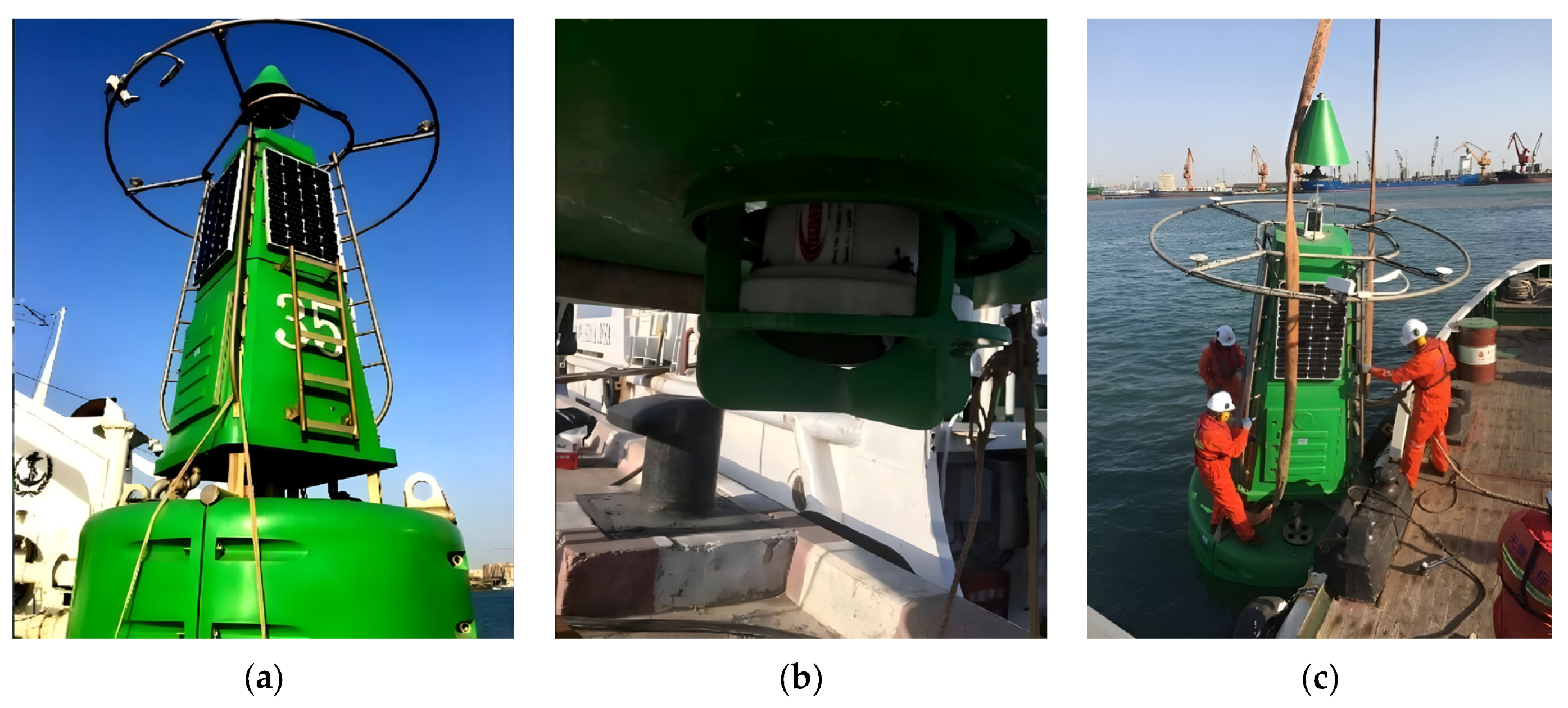
This study was inspired by an incidental observation during routine sea trials conducted in the main channel of Tianjin Port (117.92° E, 38.95° N). These trials were initially intended to evaluate the performance of instruments installed on mooring buoys (see Figure 1). A unique phenomenon was serendipitously observed: once the buoy reaches the tension limit of its chain with the incoming current, it starts to drift periodically between two extreme positions on the water surface. Simultaneously, it also rotates vertically and eventually achieves a dynamic steady state. Field observations in Tianjin Port initially revealed the pendulum-like motion. To assess its prevalence, technical interviews were conducted with the maritime manager of China Southern Navigation Service Center. Historical maintenance logs indicated that similar periodic oscillations occurred frequently, particularly in high-current zones such as the Qiongzhou Strait. This larger cross-flow motion, which was not initially anticipated, presents a challenge to the precision of data acquisition, introducing an unquantified variable into the collection process.

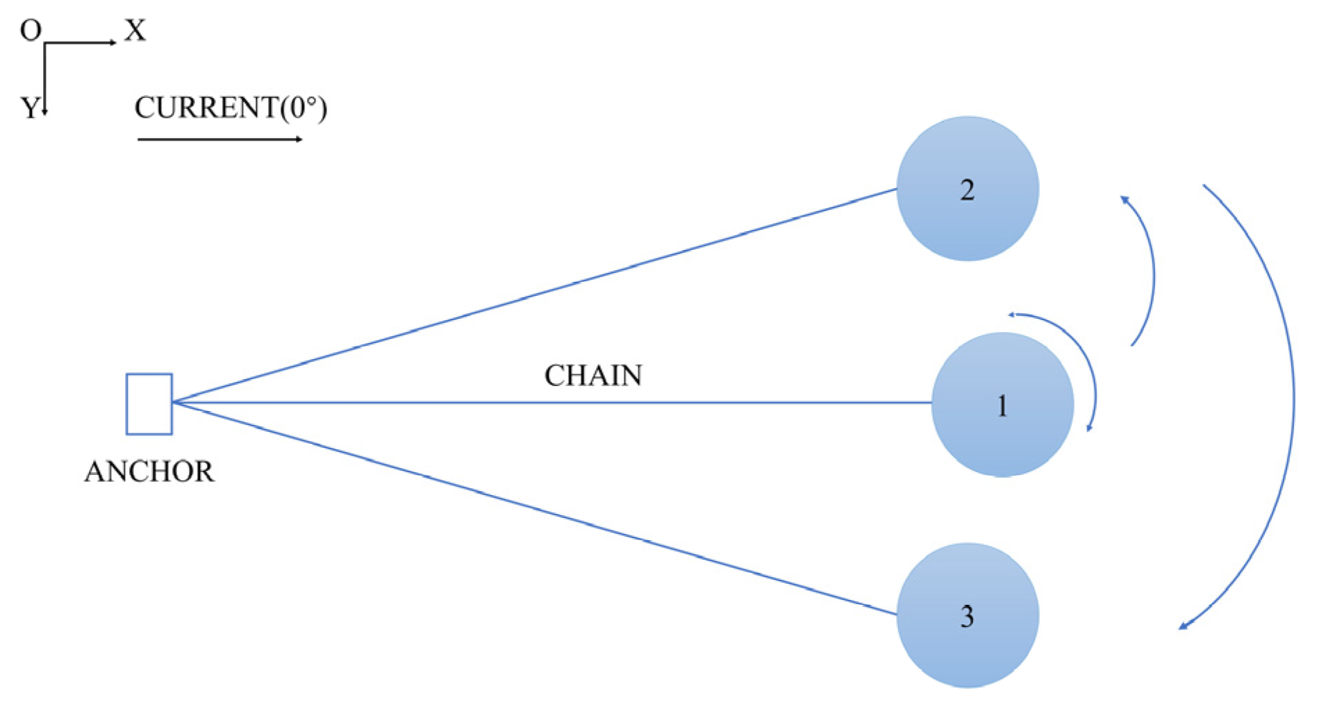
A schematic representation of this motion, as observed from an aerial perspective, is depicted in Figure 2. After the buoy drifts with the current to limit position 1, where the anchor chain tightens, it begins to move laterally from to position 2, then swings to position 3, and then returns to position 2, maintaining a stable oscillatory motion at a relatively consistent frequency. Viewed from above, this motion in question can be conceptualized as a pendulum, with the anchor point as the reference origin and the buoy acting as the pendulum’s bob. It moves along an arc-shaped trajectory on the water surface, with a radius equivalent to the projected length of the chain. Similar phenomena were occasionally observed in the laboratory model tests of the wave buoy, as documented by the authors of [2], but their research primarily examined the effect of the current on wave measurement.

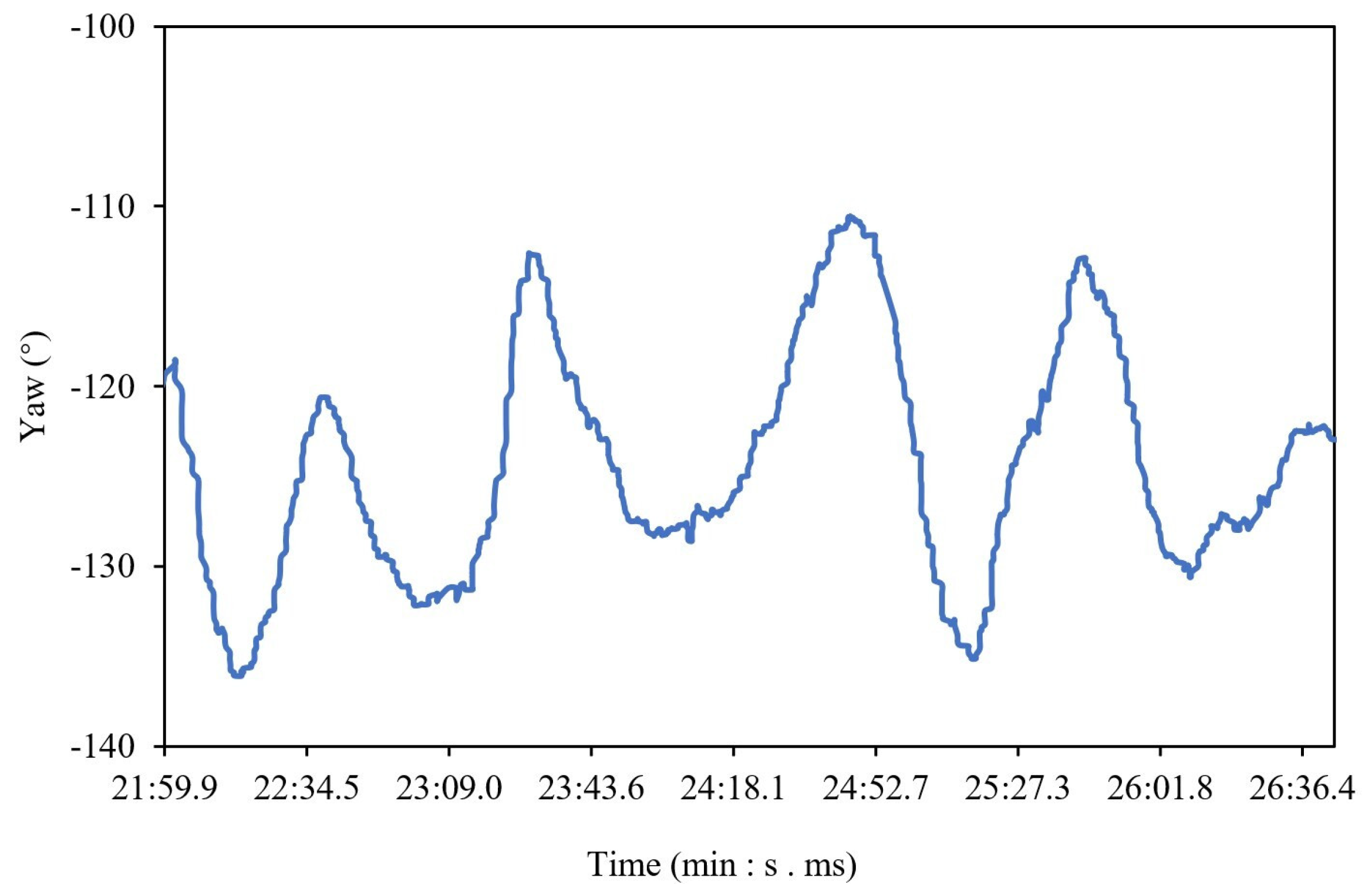
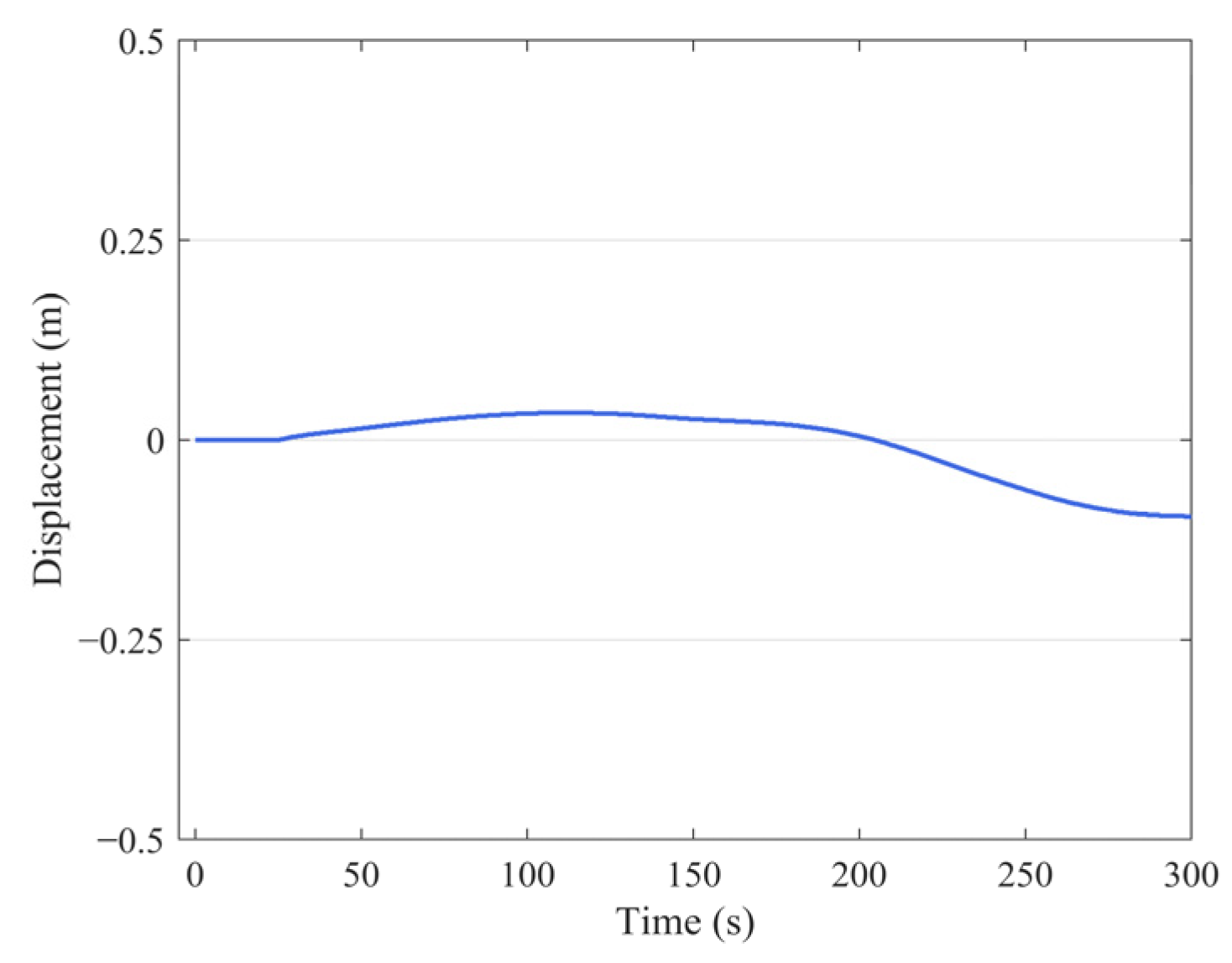
Moreover, the rapid rotation of mooring buoys can also compromise the accuracy of hydrological data. During field observations, the ADCP recorded an average current velocity of 1.16 m/s. The motion data of the buoy were collected by the MEMS-based inertial motion unit. When the buoy reached the limit position, changes in yaw were processed. As shown in Figure 3, random 300 s intervals were extracted from the overall duration. Within these 300 s spans, nearly five cycles of reciprocating variation are observed, averaging a yaw period of about 59 s. Due to limitations arising from sea conditions, the monitoring curves exhibited non-smooth characteristics. It is still evident that the buoy displays a consistent reciprocating motion. The observed rapid pendulum-like motion fundamentally differs from tidal-induced drift, which typically drives gradual displacements over hours to days. In this microtidal environment (mean tidal range: 1.05 m, Tianjin Port records), the tide acted as a quasi-steady current. Prior studies investigating tidal impacts on buoy dynamics [3,4] employed probabilistic statistics and machine learning to analyze long-term displacement trends, whereas this study specifically characterizes short-term periodic motion that operates on fundamentally different spatiotemporal scales. This intense movement of mooring buoys undoubtedly impairs the precision of sensors.

During field observations, wind speeds recorded by a calibrated anemometer (RM Young 05103) averaged 2.1 m/s, well below the threshold required to induce significant forces on the buoy. Combined with the buoy’s minimized exposed surface area above water and inherent stabilization, these conditions allowed us to attribute the motion to hydrodynamic effects rather than wind. The buoy exhibited regular back-and-forth oscillations, showing distinct periodic behavior, suggesting the presence of an alternating force acting on its structure. These force patterns align with the fundamental principles of vortex-induced vibration (VIV), a well-established phenomenon in flows past bluff bodies (such as a circular buoy). The kinematic similarity between the buoy’s motion and VIV strongly supports the hypothesis that the observed oscillations result from vortex shedding due to the similar kinematic characteristics. This interpretation underscores the necessity of accounting for fluid viscosity in subsequent analyses.

However, a substantial number of research efforts have been devoted to wave-induced heave and roll over the years, with rare attention given to the above specific dynamic issue. Potential flow theory was recognized as a standard modeling tool for predicting the responses of buoys. The study found that violent shaking or capsizing in waves poses critical threats to sensor measurement and data transmission [5]. Thus, researchers have focused on the movement under various wave conditions, with most of the models being linear [6,7,8]. Different approaches to improve the linear potential flow model have already been suggested in the literature [9,10,11]. Furthermore, the effects of viscosity are increasingly being incorporated into the analysis. By combining potential flow results with experimental data or empirical corrections, the roll motivated by viscous damping has been considered in research [12,13,14]. Unfortunately, the influence of viscous effects has not been extended to the buoy motion of other degrees of freedom.

In conclusion, although it has the potential to affect data quality and adversely disrupt ongoing monitoring efforts, this issue has received little attention in the relevant research literature. Compared to wave dynamics, the widely applied potential flow theory cannot provide better and more accurate insights into the hydrodynamic issues in viscous fluids. This unanticipated finding has spurred an investigation into the mechanisms behind this phenomenon. Experiments and numerical simulations were analyzed to elucidate the mechanisms of this periodic motion, thereby providing a basis for the correction of errors in data acquisition.

2. Driven Source of the Motion

Field observations can be influenced by many factors, such as turbulence from passing ships and the effects of reflections and refractions from offshore structures. Model tests were carried out to investigate the source of the pendulum-like motion of the buoys without these influences.

The origin of the global coordinate system was located at the position of the anchor. A right-handed coordinate system was defined with the positive x-axis pointing to the incoming current direction, the y-axis perpendicular to the incoming flow direction, and the z-axis orienting upward.

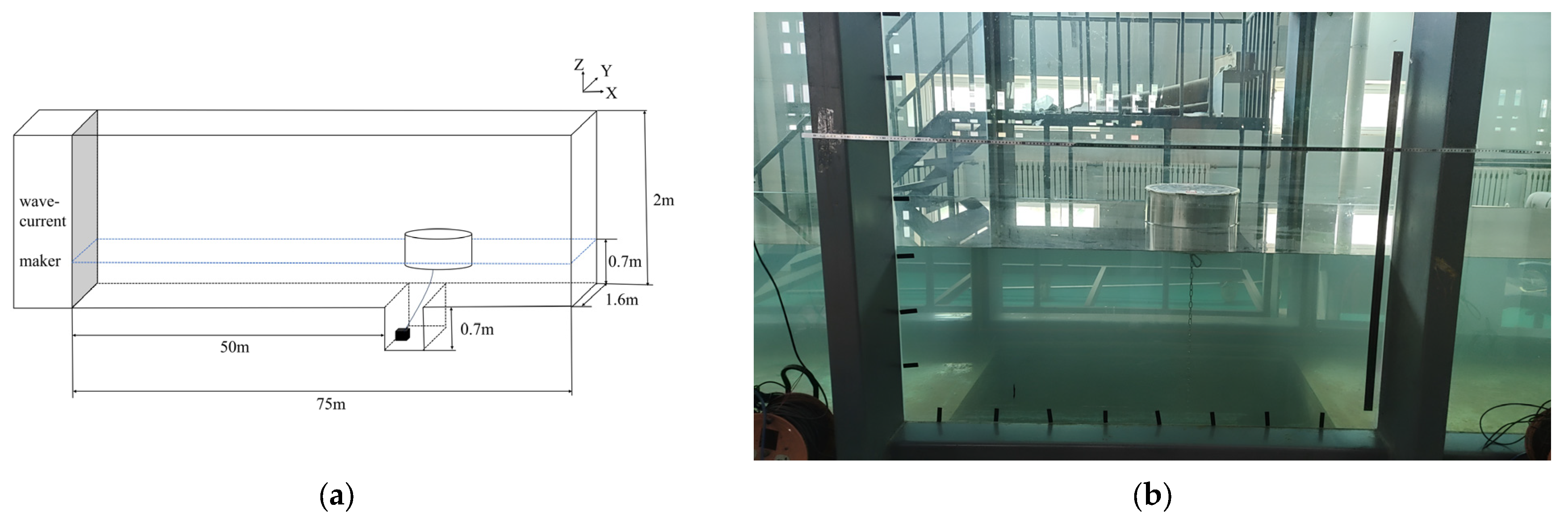
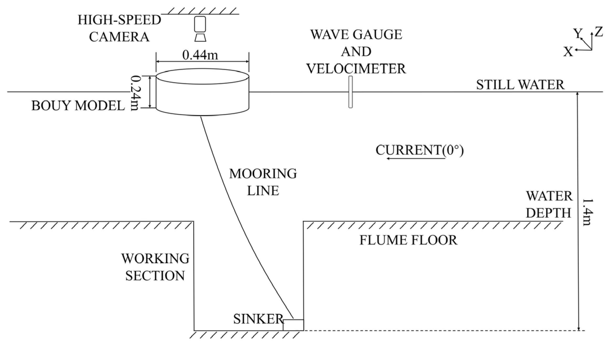
The experiments were conducted in a wave–current flume. As shown in Figure 4, the flume measures 75 m in length, 2 m in height, and 1.6 m in width. The working section is set 50 m from the wave–current maker, providing ample space for the flow to stabilize. A 0.7 m deep trench is constructed at the bottom of the working section to maximize the working water depth. The model of Buoy No. 35, used in field observations, was installed 50 m (streamwise) and 1 m (cross-flume) with a sinker. The water depth was maintained at 1.4 m for all test cases measured in the working section. It is important that the dimensions of the trench are well coordinated with the chain length, ensuring that the chain does not interact with the edges while the buoy is moving.

The model scale was reasonably determined to be 1:5, and the relevant parameters are shown in

Table 1. Floating buoy physical parameters.

Parameter	Model Data	Prototype Data
Height	0.24 m	1.2 m
Diameter	0.44 m	2.2 m
Draft Depth	0.0876 m	0.427 m
Displacement Volume	0.013 m3	1.624 m3
Mass	13.3 kg	1664.3 kg

. Some stainless ballasts were placed inside the buoy to maintain the gravity similarity law. It was deployed with a 4 mm diameter steel anchor chain, 2.5 m in length, satisfying the similarity criteria. A high-speed camera was positioned above the water surface to track the buoy’s movement and record its trajectory. As illustrated in Figure 5, a wave gauge and velocimeter were placed 5 m ahead of the model, measuring 0.2 m below the still water surface. The individual measurement sensors were integrated into the data acquisition system to maintain synchronization. All instruments had measurement validity and were strictly tested and calibrated before tests.

The experiments assessed buoy motion response under wave-only, current-only, and wave–current conditions. The purpose is to determine which fluid conditions are the driving source for the periodic pendulum-like motion. To satisfy the Froude similarity and account for laboratory current control, the comparative current speed U was set to 0.5 m/s. Regular waves, with a height H of 0.08 m and a period T of 2 s, were added as an interference factor in wave-only conditions. The combined wave–current condition was executed with waves and currents moving in the same direction along the positive x-axis. The test conditions are summarized in

Table 2. Buoy test conditions.

Test Conditions	Currents	Waves
1	0.5 m/s	/
2	/	H = 0.08 m, T = 2 s
3	0.5 m/s	H = 0.08 m, T = 2 s

.

The experiment started once the cross-sectional velocity was confirmed to be stable under the test conditions by a velocimeter. Every oscillation experiment was carried out three times, with each condition being recorded for 300 s to obtain statistically average results. As expected, the buoy moved downstream to its limit position where the anchor chain was tightened. The chain projection length on the water surface is about 2 m. Subsequently, the displacement in the x-direction was found to be negligible, while the positional changes in the y-direction dramatically increased. The cylinder was constrained to move along an arc with a radius equivalent to the projected length of the anchor chain (2 m). 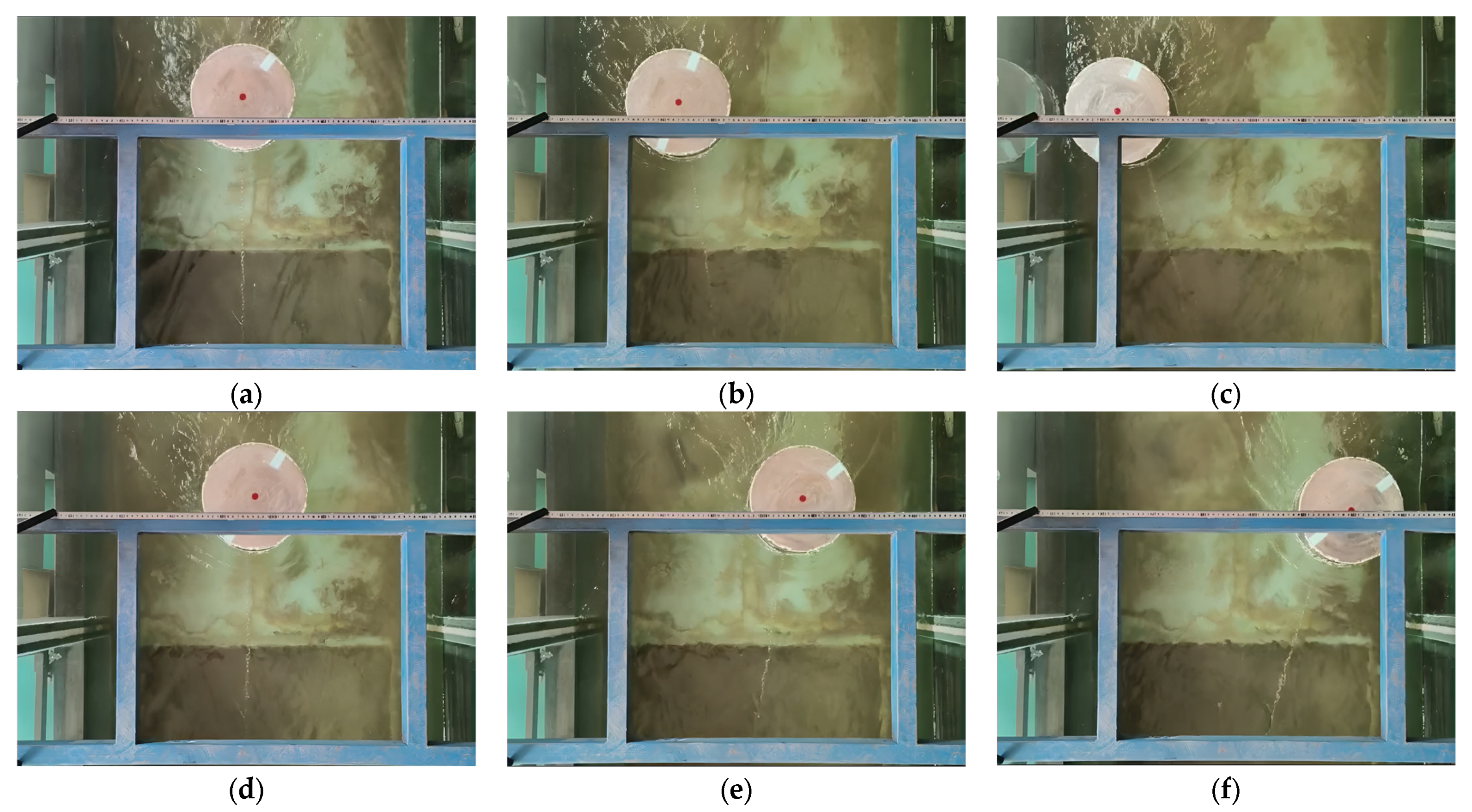As shown in Figure 6, all motion processes were captured by a high-speed camera. The time series data of the model’s displacements were presented after correcting for lens distortion. The commencement time was recorded from the moment the commands were transmitted to the current maker, which led to an initial phase of unstable current velocity. Therefore, only data subsequent to the 50 s mark were subjected to analysis.

The results from Test 1, as presented in Figure 7, clearly demonstrate that severe motion resembled that of a pendulum observed over time in the current-only condition. It shows a periodic translational movement, marked by repeated movement from side to side along a relatively fixed path. The pulsating effects of turbulence at high flow speeds lead to random flow fluctuations, resulting in a pulsating motion of the buoy. When the buoy approached the sidewalls of the flume, the hydrodynamic effects in the near-wall region further complicated its motion trajectory. These motions are much more complex than those observed for submerged and semi-submerged bodies with fixed mountings [15,16], yet despite this, periodic oscillation was found to occur as previously reported. Although the movement is not simply arc-shaped as a pendulum motion, the overall trend in the transverse direction remains periodic. The maximum oscillatory displacement, defined as the most significant movement of the model from one side of the flume to the other (i.e., the distance between the highest and lowest points presented in the graph), is used to characterize the extent of the periodic oscillation. This maximum oscillatory displacement in the current-only condition reaches approximately 1.21 m, with an average completion time of just 21 s. The dynamic response of the model was characterized by high frequency, high velocity, and large-amplitude vibrations.

Assessing the y-direction displacement in the wave-only condition in Figure 8, it is evident that the y positions of the buoy are almost unchanged and negligible and show low frequency. It almost remained constant for the entire wave run. The amplitude of oscillation was small compared to the diameter of the buoy. It seems that the rapid drift of buoys was uncorrelated to wave forcing.

Considerable differences were observed when comparing buoy motions in wave-only conditions to those in the same input wave conditions following a 0.5 m/s current (see Figure 9). Large periodic oscillation, i.e., the side-to-side pendulum-like motion reemerged with the introduction of current. This general state concurs with the findings in current-only conditions. Therefore, it was concluded that the pendulum-like motion is still present in the presence of waves. Collinear waves do not appear to impede the periodic movement remarkably. Compared to current-only conditions, couple-load conditions characterize complex nonlinear responses. Despite the unstable motion of the buoy, the displacement in the y-direction was also noticeable. The peak-to-peak amplitude of the oscillation is approximately 0.51 m, with a maximum oscillatory displacement of about 1.11 m. The stability of the mooring system is relatively weak, and after the current stabilizes, the average period of the turbulent pulsation oscillations is around 15 s. Based on the displacement in the y-direction, the collinear wave reduced the amplitudes of motion, a finding that is consistent with Finnigan’s research on the behavior of multi-column truss platforms [17].

The laboratory experiments clearly demonstrate that the current induces severe cross-flow motion, characterized by considerable amplitude and high frequency. It has been observed that the buoy model oscillates dramatically solely under the influence of the current. This motion was attributed to the action of currents and was independent of wave activity. The reason for the rapid reciprocating drift of buoys only occurring in the presence of the current is further explored in Section 3.

3. Mechanisms of the Motion

Based on the detailed response analysis in Section 2, the current induces a cross-flow motion of the buoy. This section aims to investigate why the pendulum-like motion occurs exclusively in the presence of the current. Since the interest is in elucidating the mechanisms, a comparative study of buoy responses is not the central theme of our model. Instead, the numerical approach complements the experimental findings by providing a more profound analytical insight. As postulated in Section 1, the observed phenomenon likely stems from periodic vortex shedding. To rigorously assess this hypothesis, a viscous computational fluid dynamics (CFD) model—capable of explicitly resolving the unsteady vortex dynamics—will be employed to validate the hypothesized mechanism and quantify its contribution to the flow instability.

The Reynolds-averaged Navier–Stokes (RANS) model was employed to obtain time-averaged flow fields. The fluid properties such as velocity and pressure are decomposed into average and fluctuating (turbulent) components. The RANS equations, together with the continuity equation, form a closed system of nonlinear equations used to describe complex fluid motion:

$${\displaystyle \frac{\partial \overline{u_i}}{\partial x_i}}=0$$

(1)

$${\displaystyle \frac{\partial \overline{u_i}}{\partial t}}+\overline{u_j}{\displaystyle \frac{\partial \overline{u_i}}{\partial x_j}}=-{\displaystyle \frac{1}{\rho }}{\displaystyle \frac{\partial \overline{p}}{\partial x_i}}+\nu {\displaystyle \frac{{\partial }^2\overline{u_i}}{\partial x_j\partial x_j}}-{\displaystyle \frac{\partial \overline{u_i^{\prime }{u}_j^{\prime }}}{\partial x_j}}$$

(2)

Equations (1) and (2) are the Reynolds-averaged governing equations, where $\overline{u_i}$ represents the time-averaged velocity components, $\rho$ is the density, $\overline{p}$ is the time-averaged pressure, $\nu$ is the kinematic viscosity, and $\overline{u_i^{\prime }{u}_j^{\prime }}$ is the Reynolds stresses. The $k-\omega$ Shear Stress Transport (SST) Turbulence Model was chosen as a baseline closure model [18]. The $k-\omega$ SST model combines the accuracy of $k-\omega$ near walls with $k-\epsilon$ in free-stream flows, enabling robust predictions of complex turbulence, separation, and shear layers across diverse engineering applications. Its performance in similar hydrodynamic applications has been extensively documented [19].

The $k-\omega$ SST model includes two additional transport equations to represent the turbulent characteristics of flow. One of the transported variables is the turbulent kinetic energy $k$:

$${\displaystyle \frac{\partial }{\partial t}}\left(\rho k\right)+{\displaystyle \frac{\partial }{\partial x_i}}\left(\rho k{\overline{u}}_i\right)={\displaystyle \frac{\partial }{\partial x_j}}\left({\mathrm{\Gamma }}_k{\displaystyle \frac{\partial k}{\partial x_j}}\right)+G_k-Y_k\left(i,j=1,2,3\right)$$

(3)

The second is the specific dissipation rate $\omega$:

$${\displaystyle \frac{\partial }{\partial t}}\left(\rho \omega \right)+{\displaystyle \frac{\partial }{\partial x_i}}\left(\rho \omega {\overline{u}}_i\right)={\displaystyle \frac{\partial }{\partial x_j}}\left({\mathrm{\Gamma }}_{\omega }{\displaystyle \frac{\partial \omega }{\partial x_j}}\right)+G_{\omega }-Y_{\omega }+S_{\omega }\left(i,j=1,2,3\right)$$

(4)

where ${\mathrm{\Gamma }}_k$ and ${\mathrm{\Gamma }}_{\omega }$ are the effective diffusion coefficients for $k$ and $\omega$, respectively,$G_k$ and $G_{\omega }$ are the production terms for them, and $Y_k$ and $Y_{\omega }$ are the turbulent dissipation terms. $S_{\omega }$ is the cross-diffusion term.

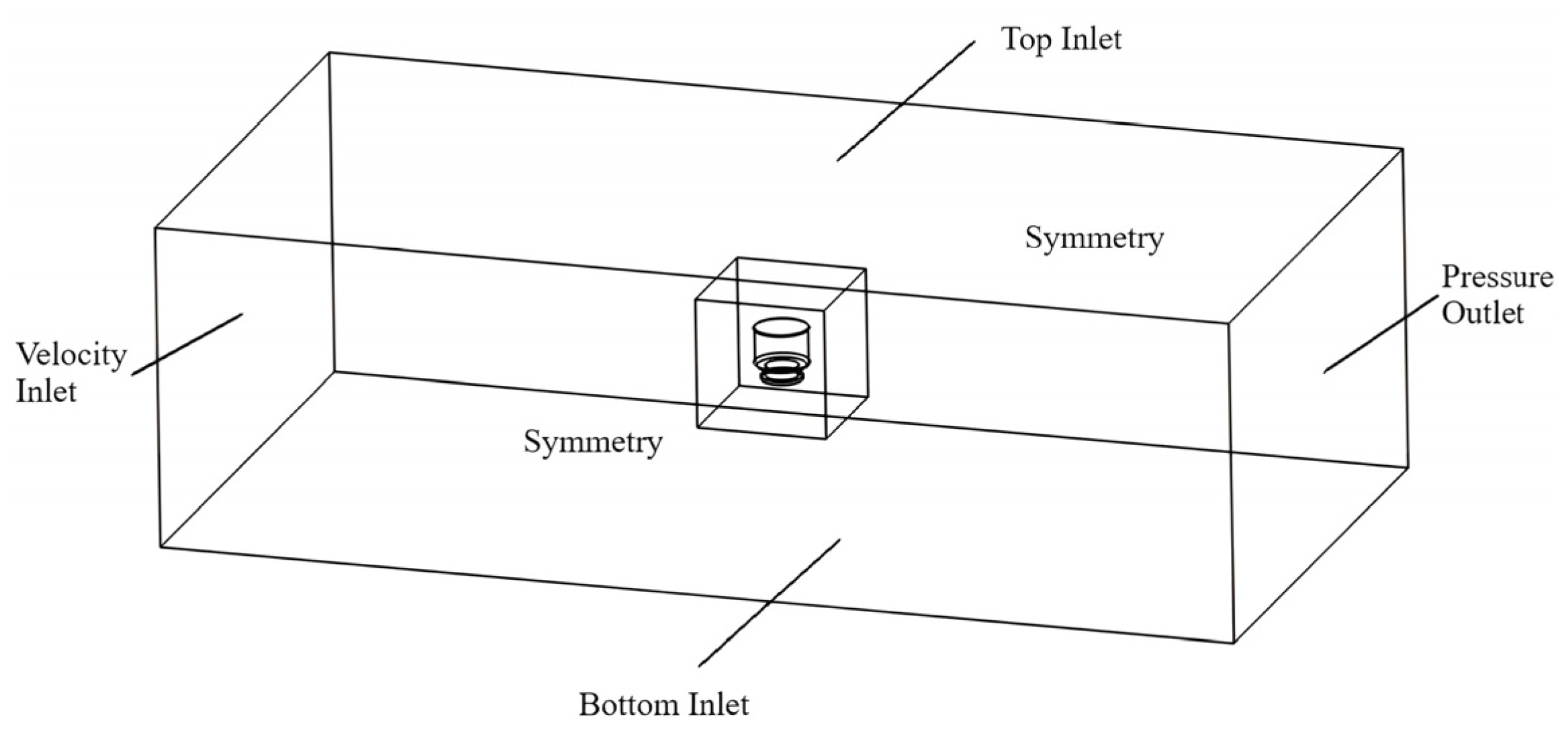
In this section, the numerical model focuses on the hydrodynamic action of buoy in the current-only condition. To isolate the effects of viscous flow, the upper aerodynamic loads and wave actions were excluded from the simulation. So, the research objective was simplified to a cylinder, constructed using the 3-CAD-Model module in STAR-CCM+ software(version 2020.2.1 Build 15.04.010 R8 Double Precision, Win/Linux 64-bit). The buoy is partially submerged, with its draft and mass distribution calibrated to match the prototype No. 35 buoy used in field observations. It is crucial to mention that, although guardrails and brackets were not explicitly modeled, their contributions to the total mass, inertial moments, and center of gravity were incorporated to ensure consistency with the prototype parameters.

Simulation parameters were chosen based on the corresponding field observations. Figure 10 shows the setting of boundary conditions, where the left side is the velocity inlet, and the right side is the pressure outlet. Moreover, symmetric boundary conditions are applied for the domain bottom and the two lateral walls. The free surface was treated as symmetric to eliminate wave effects, allowing the study to concentrate on current-driven forces.

Grid overlapping was adopted to discretize the progressively complicated boundary shapes. It can divide the flow domain into two regions: one is the fixed background region encompassing the whole flow field, and the other one is the grid close to the research objective which moves with a buoy (as shown in Figure 11). The grids communicate through data transference by an interpolation procedure.

The STAR-CCM+ solves RANS equations through its advanced built-in numerical solvers. It calculates the detailed pressure distribution over the buoy’s surface at every timestep. Based on Newton’s Second Law, the software solves the rigid body motion equation of a floating body through a six-degree-of-freedom (6-DOF) model. We only need to provide physical parameters and define degrees of freedom and external force constraints.

The mooring chain was simplified as a geometric constraint with a fixed anchor point, and the fluid forces (drag and lift) were integrated over the buoy surface. The mooring system of the buoy comprises a single cable. One end is fixed to the fairlead at the buoy’s base, and the other is anchored to the seabed. The cable forms a catenary under gravity, buoyancy, and tension.

Assuming the cable is elastic (Hooke’s law), with uniform submerged weight (constant linear density) and negligible bending and torsion, the equilibrium of a differential cable segment satisfies

$${\displaystyle \frac{dT}{ds}}=w\sin \theta$$

(5)

$$T{\displaystyle \frac{d\theta }{ds}}=w\cos \theta$$

(6)

where $T$ is tension, $w$ is submerged weight per unit length, and $\theta$ is the angle from the horizontal. Introducing the dimensionless parameter $\xi =s/L_0$ ($L_0$ is unstretched length) and integrating yields the following parametric equations:

$$x(\xi )=H\left({\displaystyle \frac{\xi }{EA}}+{\displaystyle \frac{{\sinh }^{-1}(V/H)}{w}}\right)$$

(7)

$$y(\xi )={\displaystyle \frac{H}{w}}\left(\cosh \left({\displaystyle \frac{w\xi }{H}}\right)-1\right)$$

(8)

where $H$ is horizontal tension, $EA$ is axial stiffness, and $V$ is vertical tension.

STAR-CCM+’s Catenary Coupling module solves these equations iteratively. Boundary conditions at the anchor ($\xi =0$) and fairlead ($\xi =1$) yield nonlinear equations for $H$ and $V$, resolved at each timestep.

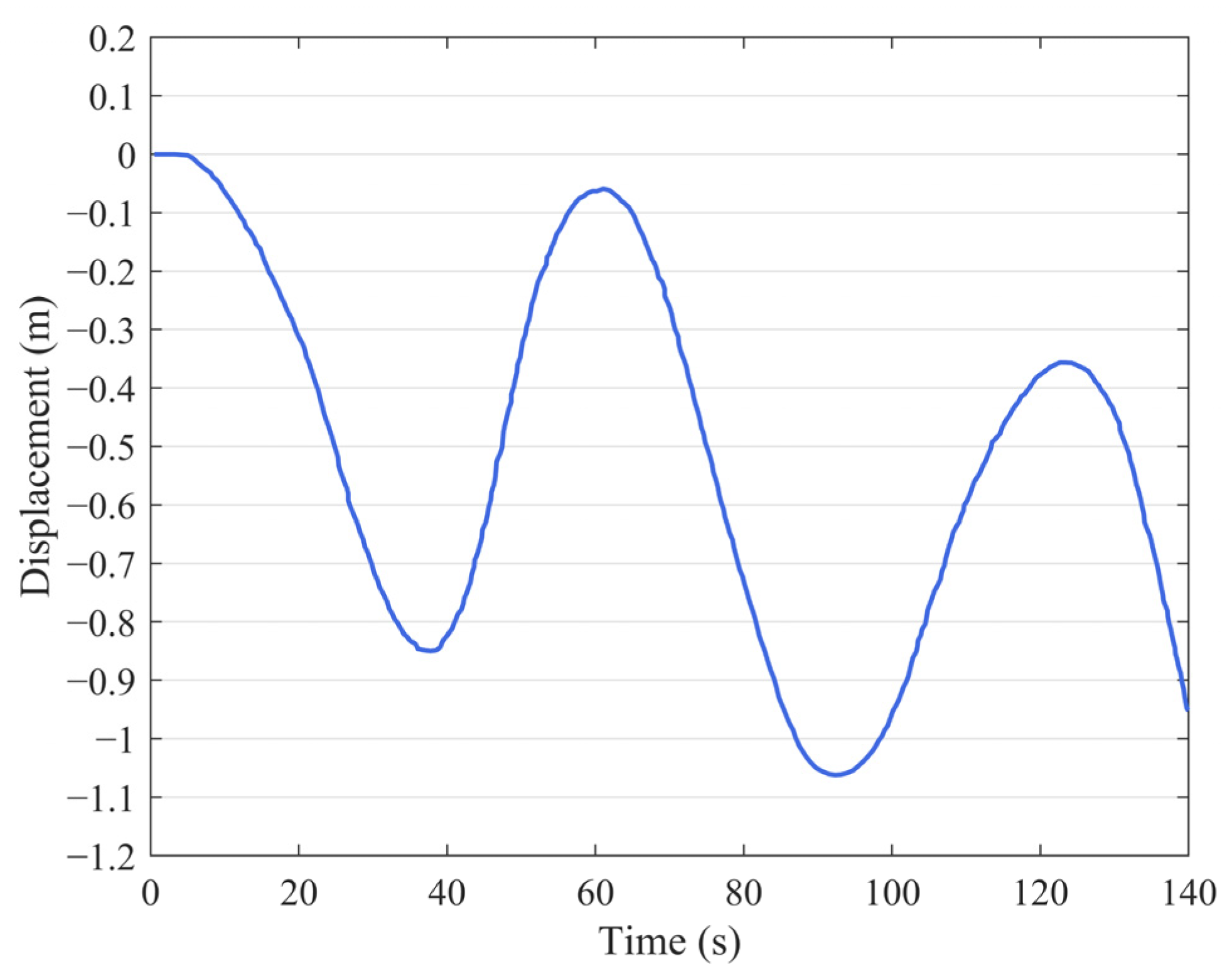
The incident current velocity was set to 1.16 m/s, which is consistent with the average velocity measured in field observation. As expected, initially, the model drifted downstream to its limit position, and it began to sway violently parallel to the y-direction, as drawn in Figure 12. The turbulent fluctuations at all scales in the instantaneous flow field are effectively eliminated using the Reynolds-averaged method. The numerical results were obtained in a relatively stable mean flow field. Therefore, comparing these results to the laboratory findings, it can be observed that the numerical simulations lack the random velocity fluctuations induced by pulsation effects, presenting a smoother trajectory. The buoy reciprocating oscillates between two extreme positions, with two complete periodic motions occurring within a 140 s timeframe and the initiation of the third period at the 123 s mark.

Comparing the field experimental data in Figure 3 with the numerical simulation results presented in Figure 12, it is evident that both exhibit periodic motion characteristics. A detailed comparison of the oscillation frequencies associated with these motions was conducted. For the y-direction displacement in numerical simulation, the buoy completed two full cycles and an additional one-third cycle within a 140 s duration, yielding an average period of 60 s. For the yaw of the field experiment, despite the presence of numerous influencing factors, the buoy experienced four full cycles plus two-thirds of a cycle over a 280 s interval, with an average period of 59 s. The reciprocating oscillation is also coupled with yaw at a visually similar frequency; the trend of both is almost identical. This can indicate that reciprocating motion and yaw are driven by the same excitation force. In other words, the buoy yaws and sways simultaneously when subjected to a specific excitation force in the current. Both movements are periodic and repetitive, continuing with the incoming flow.

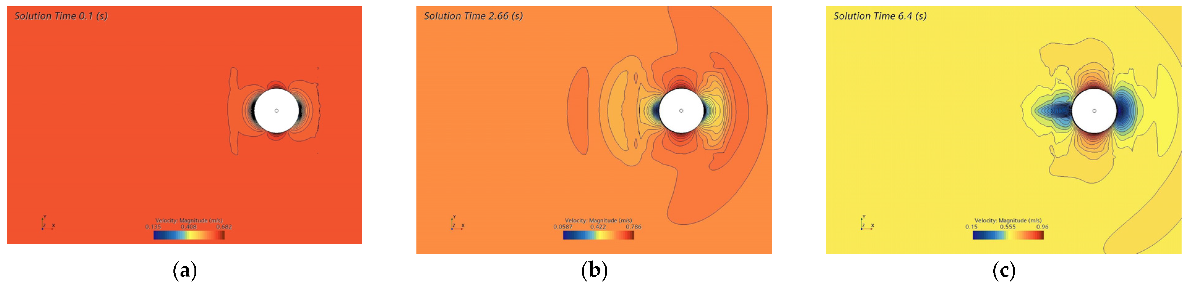
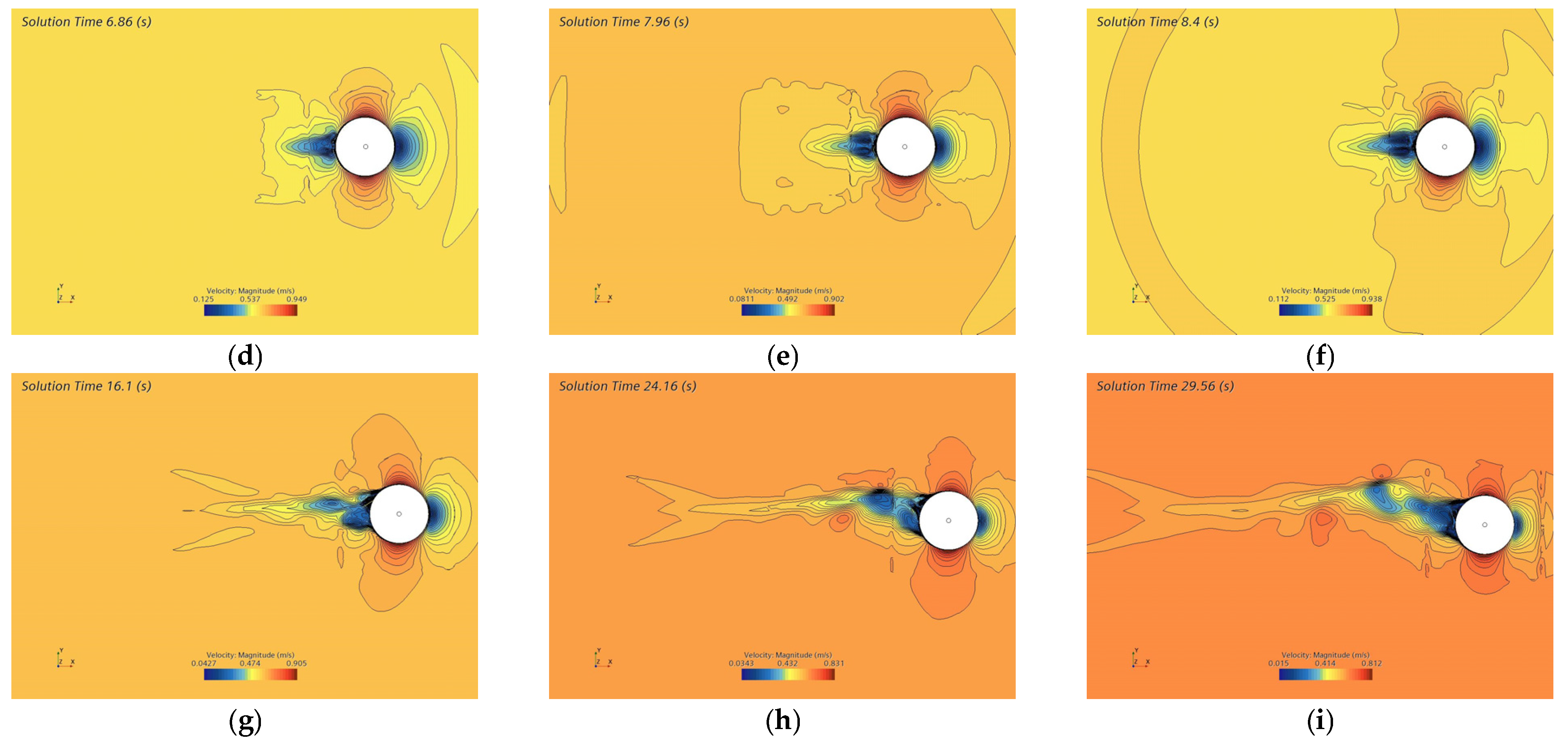
To clarify and enhance the intuitive understanding of this argument, a simulation was conducted to recognize and obtain the instantaneous flow patterns behind the bluff body in the flow field. The results shown in Figure 13 illustrate the instantaneous variations in the scalar velocity profile, which captures the sequential processes from vortex formation to their eventual dissipation. The evolution of vortex structures is clearly depicted, a phenomenon that is inherently challenging to fully capture or observe in laboratory settings due to measurement limitations. A portion of the flow field was extracted for imaging, with the snapshots taken at intervals of approximately one shedding period. This allows for a deeper understanding of the dynamics between vortex shedding, and the periodic pendulum-like motion of the buoy. As a result, the simulation provides a more robust validation of the mechanisms that govern periodic motion, enhancing the fidelity of the experimental outcomes.

As can be seen from Figure 13a, a boundary layer occurs on the surface of the buoy at the initial time when fluid flows through it. The flow speed is faster on the upper and lower surfaces of the buoy, while it is slower on the front and rear surfaces. Figure 13b,c illustrates the transition process of a separated boundary layer, with some vortices gathered and attached to the back of the cylinder. According to Figure 13d, at time 6.86 s, a pair of counter-rotating vortices forms and attaches vertically upward and downward around the cylinder. Figure 13e shows that the vortex began to fall off at time 7.96 s. At time 8.4 s, the previously formed vortices have completely shed from the cylinder, forming new vortices (Figure 13f). As these vortices detach from one side of the buoy, a low-pressure area is formed on the opposite side. The uneven distribution of forces results in the buoy moving in the direction of the side where the vortex has recently separated. Subsequently, new vortices form and detach on the opposite side of the buoy. The vortices were built up and released from the body during the large sway accelerations when it moved in its wake. Figure 13g shows that after 16.1 s, vortices alternately shed from the trailing edge of the cylinder, developing into two parallel rows; that is, the vortex street behind the buoy began to form. At 24.16 s the vortex street was fully developed, and the shed vortices coalesced in the buoy’s wake (see Figure 13h), simultaneously exerting periodic forces.

The vortex shedding frequency was analyzed using the Strouhal number (St), defined as

$$St={\displaystyle \frac{f\cdot D}{U}}$$

(9)

where $f$ is the shedding frequency, D = 2.2 m is the cylinder diameter, and U = 1/16 m/s is the current velocity. Experimental observations from image time-series data (7.96 s to 24.16 s) revealed approximately two full shedding cycles, yielding a frequency of 0.123 Hz. Substituting the parameters into the equation results in a value of St = 0.23.

The Reynolds number for water (${\nu }_{water}=1\times {10}^{-6}{\mathrm{m}}^2/\mathrm{s}$) was calculated as

$$Re={\displaystyle \frac{UD}{{\nu }_{\mathrm{water}}}}\approx 2.55\times {10}^6$$

(10)

indicating a supercritical flow regime $(Re>3\times {10}^5)$ with turbulent boundary layer separation. While supercritical flows often exhibit slightly elevated St values (0.25–0.3), the measured St number remains close to theoretical expectations. Minor deviations may arise from simplified turbulence modeling or surface roughness effects influencing separation dynamics. The results demonstrate good agreement with theoretical St ranges for cylindrical flows.

Throughout the process, the buoy drifts from side to side. When viewed from above, this manifests as a pendulum-like oscillation, as depicted in Figure 14. The mooring buoy experiences tangential drag force $F_d$ in the x-direction, resulting in the body yawing, while simultaneously experiencing a lift force, $F_l$, in the y-direction. The buoy is assumed to initiate a clockwise movement from equilibrium position 1 under the influence of the resultant force. During this phase, lift force $F_l$ gradually decreases until it reaches equilibrium with the combined force of fluid resistance and mooring forces at extreme position 2. It then begins to move counterclockwise until it arrives at position 3 where a new force equilibrium is achieved. Based on the above analysis, the periodic oscillation force of the buoy can be decomposed into two directions, and the total motions are found to depend on the vortex-induced forces along with the mooring restoring forces. These vortices induce the periodic variation in lift and drag forces on the surface of the cylinder. The fluctuating forces from vortex shedding result in a pendulum-like motion from an aerial view. The formed vortex street is not straight, as shown in Figure 13i. Because the body moves periodically in the y-direction, it exhibits an oscillatory pattern akin to a “fishtail”, synchronized with the periodic motion of the buoy.

The numerical simulation further clarifies the answer: the oscillatory forces from vortex shedding are an essential source of the pendulum-like motion on the water surface. The phenomenon of vortex shedding is fundamentally rooted in viscous fluid dynamics through its governing role in boundary layer behavior. It is the viscous shear stresses within the fluid that enable the formation of a boundary layer adhering to solid surfaces. When the flow velocity reaches critical conditions, viscous dissipation accumulated within this boundary layer triggers flow separation. The separated shear layer subsequently rolls up into discrete vortices through the competing action of inertial forces and residual viscous stresses. This confirms that viscosity governs both the flow separation, vortex shedding, and the structural motion, processes that inviscid potential flow models fundamentally cannot capture. The absence of boundary layer physics and surface friction modeling in these simplified frameworks explains their failure to predict such phenomena. Therefore, any refinement of buoy trajectory mathematical models must explicitly incorporate these viscous effects.

The pendulum-like motion significantly impacts the collection and transmission of data by the sensors equipped on the buoy. By establishing fluid viscosity as the critical factor maintaining vortex patterns and their force impacts, these findings expose a key limitation of non-viscous models in predicting fluid–structure interactions. This study not only identifies vortex shedding as the primary driver of buoy pendulum-like motion but also emphasizes the need to account for viscous effects when modeling buoy behavior.

4. Discussion

The investigation into the pendulum-like motion of buoys was initially prompted by concerns over its potential impact on the quality of data collection. This motion can also engender other issues. This unexpected movement poses a hazard to the safety of passing ships. Mooring buoys exhibit strong susceptibility due to the difficulty in providing a significant restoring force with a single cable. It is imperative to recognize that a substantial number of collisions between ships and buoys are still reported annually [20]. This is attributed to the high moment of inertia and notable blind spots of ships, which necessitate a specific amount of time and distance, known as advance distance, to change direction when the rudder is engaged [21].

Recent incidents in the South Channel of Shanghai (China Pudong Maritime Safety Administration 2024) further validate these risks. The tugboat “Zhong XXX” collided with the S11 buoy during towing operations, causing its towed vessel “Rui XXX” to snag and drag the buoy. An investigation revealed that the buoy’s rapid pendulum-like motion caused it to approach the vessel unexpectedly. The crew failed to anticipate the buoy’s erratic trajectory, leading to the hasty application of the full rudder. This emergency steering worsened the ship’s stern swing toward the buoy. While human error (e.g., unfamiliarity with local currents) played an important role, the buoy’s large-amplitude pendulum-like motion was also identified as a primary contributor.

These incidents underscore the operational hazards posed by vortex-driven buoy oscillations, particularly in narrow channels where rapid drift leaves minimal time for collision avoidance. Ref. [22] indicates that even if there is no collision, the maximum tension in the mooring lines during drift can increase dramatically. This sharp rise in tension may lead to line breakage. If a buoy breaks free from its mooring, it can lead to increased maintenance frequency for sensors and economic losses. Our study’s focus on viscous effects and vortex shedding mechanisms aligns with these real scenarios, emphasizing the need to predict and mitigate such motions.

As discussed, the phenomenon of pendulum-like motion in mooring buoys poses significant challenges to offshore engineering operations. However, the characteristics of mooring buoys have not garnered adequate scholarly attention yet. Some studies have ventured to explore the drift movement of large deep-draft structures, such as semi-submersible platforms with multiple columns [23,24,25]. There are also investigations concerning the unique motion characteristics of Spar [26,27]. These platforms have relatively large aspect ratios (draft over diameter) and are equipped with multiple mooring lines for attachment. The above structures have substantial differences in structural design and mooring methodologies when compared to the focus of our study. Single-cable mooring buoys, being the most common type of marine facility, have not been thoroughly analyzed for their rapid cross-flow motion. Consequently, it has become imperative to consider the impact of viscosity on its horizontal movement in studying buoy motion.

The ultimate solution for addressing the challenges posed by the pendulum-like motion of buoys lies in the ability to predict this movement accurately. The initial phase in this predictive endeavor is to comprehend its mechanism, which has been delineated through laboratory experiments and numerical simulations presented in this paper. Following this, a critical step involves the analysis of the factors that influence this motion. It is vital to point out that our work only provides a preliminary exploration of the impact of current speed on the pendulum-like motion of buoys. In the experiments presented, the motions in current-only conditions were found to depend on the vortex-induced forces along with the mooring restoring forces. To extend these findings, several avenues warrant further investigation:

(1)

Mooring System: Both the frequency and amplitude of motions were significantly affected by the mooring system. The weight and acceleration of the mooring chains are identified as critical factors that significantly influence dynamic behavior, especially for movements of lower periods and higher amplitudes [28]. Additionally, the length and elasticity of the anchor chain altered the dynamic equilibrium between the restoring forces and the oscillatory forces arising from vortex shedding, highlighting the need for a holistic understanding of mooring–buoy interactions. Comparative studies across varying depth-to-chain-length ratios are also essential to optimize buoy stability in diverse marine environments. Integrating adaptive mooring designs (e.g., multi-line configurations or elastic materials) may mitigate adverse motions.

(2)

Current Velocity Variability: A systematic analysis of how varying current velocities (e.g., subcritical vs. supercritical regimes) modulate vortex shedding frequencies and buoy response is needed. Such investigations could inform predictive models for extreme flow conditions. Such investigations should concurrently address water depth effects, as deeper environments amplify mooring line hydrodynamic complexities that traditional quasi-static models often underestimate [29].

To summarize, these factors exert a great influence on the amplitude and frequency of the cross-flow oscillation. A detailed study of these factors could be an interesting aspect of future research. The objective is to predict the response of the pendulum-like motion through the integration of these determinants into predictive models.

5. Conclusions

With the growing demand for high-accuracy marine data acquisition, the mooring buoy, as a widely used tool, has received more attention. The predictable dynamic responses of buoys play a critical role in ensuring accurate and continuous collection. Through the field observations, it was found that the buoy undergoes regular periodic movement between two extreme positions, similar to a simple plane pendulum from an aerial perspective. This rapid and large motion increases the gaps in data acquisition and relatively large errors. This study focuses on this drift motion induced by the viscous effects, and the main conclusions are as follows:

(1)

Through scaled testing (circa 1:5) in a combined wave–current test flume, the motion behavior characteristics were compared in wave-only, current-only, and wave–current conditions. The model has large, rapid, and complex y-motions exceeding the buoy diameter in the current condition. There is no y-forcing from the waves. It is shown that the dramatic motion was induced by the current and was unrelated to the waves.

(2)

The directly visualized numerical results were presented to investigate the mechanism of this motion. The instantaneous flow patterns behind the bluff body in the flow field were presented. Vortices continuously separate from the surface of the buoy as it undergoes periodic motion. The detailed evidence reveals that the oscillating force from vortex shedding in viscous flows is the driving force that contributes to the pendulum-like motion. This confirms that the pendulum-like motion of the buoy is a manifestation of VIV. The oscillatory forces generated by alternating vortex shedding from the buoy’s surface drive the periodic pendulum-like motion, while the mooring chain acts as a restoring force analogous to a spring in classical VIV systems. The interplay between vortex shedding and mooring stiffness governs the oscillation amplitude and frequency. This may bridge the gap between traditional VIV studies—typically focused on elastically mounted cylinders—and the practical behavior of moored marine structures, underscoring the universality of vortex-driven dynamics in fluid–structure interactions.

The results emphasize that fluid viscosity and the resulting vortex effects have a remarkable impact on buoy motion characteristics, an aspect that seems to have received limited attention in previous studies. Considering the influence of fluid viscosity could potentially enhance the understanding of buoy responses, which can provide a foundation and hold potential for addressing more applied problems, for instance, in data error-correcting and trajectory predictions. Specifically, frequency domain filtering techniques could isolate and suppress pendulum-like motion artifacts in accelerometer signals. For trajectory prediction, coupling hydrodynamic lift force models with existing mooring dynamics equations may enhance predictive robustness across unsteady flow regimes. This study makes an effort to draw broader attention from the academic and engineering communities to the impact of fluid viscosity on buoy motion, hoping to inspire further theoretical validation and experimental research.